Author Contributions
Conceptualization, C.-G.L. and Z.-P.W.; methodology, H.-G.W., L.-F.H. and L.-J.Z.; software, L.-F.H. and L.-J.Z.; validation, L.-F.H. and Z.-P.W.; formal analysis, C.-G.L. and H.-G.W.; investigation, H.-G.W., L.-F.H. and L.-J.Z.; resources, C.-G.L. and Q.-L.Z.; data curation, J.H. and L.-F.H.; writing—original draft preparation, L.-F.H. and L.-J.Z.; writing—review and editing, Z.-P.W., M.-C.S. and C.-G.L.; visualization, L.-F.H. and L.-J.Z.; supervision, Z.-P.W. and Q.-L.Z.; project administration, C.-G.L. and Q.-L.Z.; funding acquisition, H.-G.W. and M.-C.S. All authors have read and agreed to the published version of the manuscript.
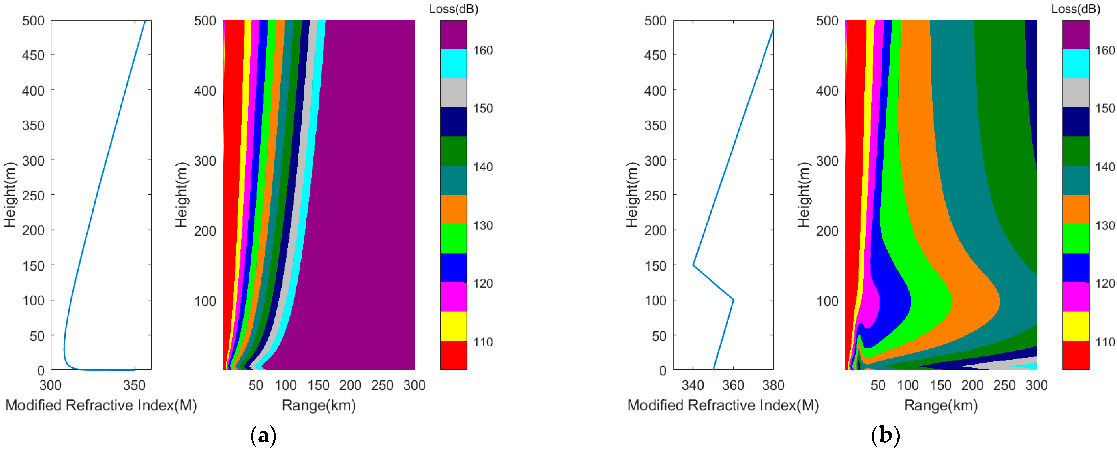
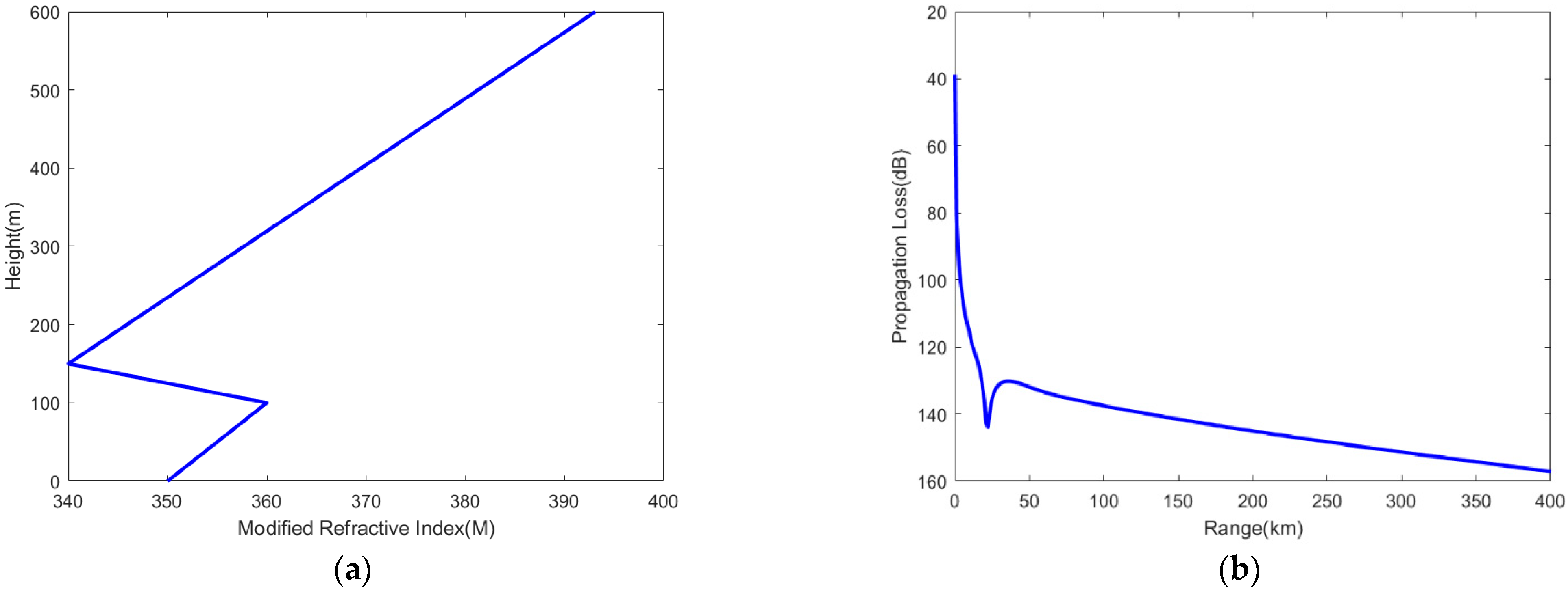
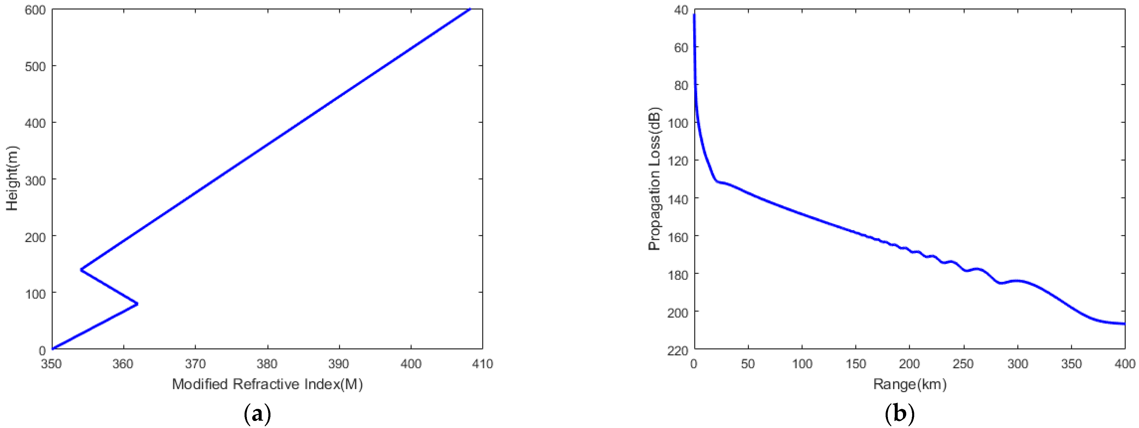
Figure 1.
Atmospheric modified refractive index profiles and AIS signal propagation loss diagram. (a) Evaporation duct; (b) lower atmospheric duct.
Figure 1.
Atmospheric modified refractive index profiles and AIS signal propagation loss diagram. (a) Evaporation duct; (b) lower atmospheric duct.
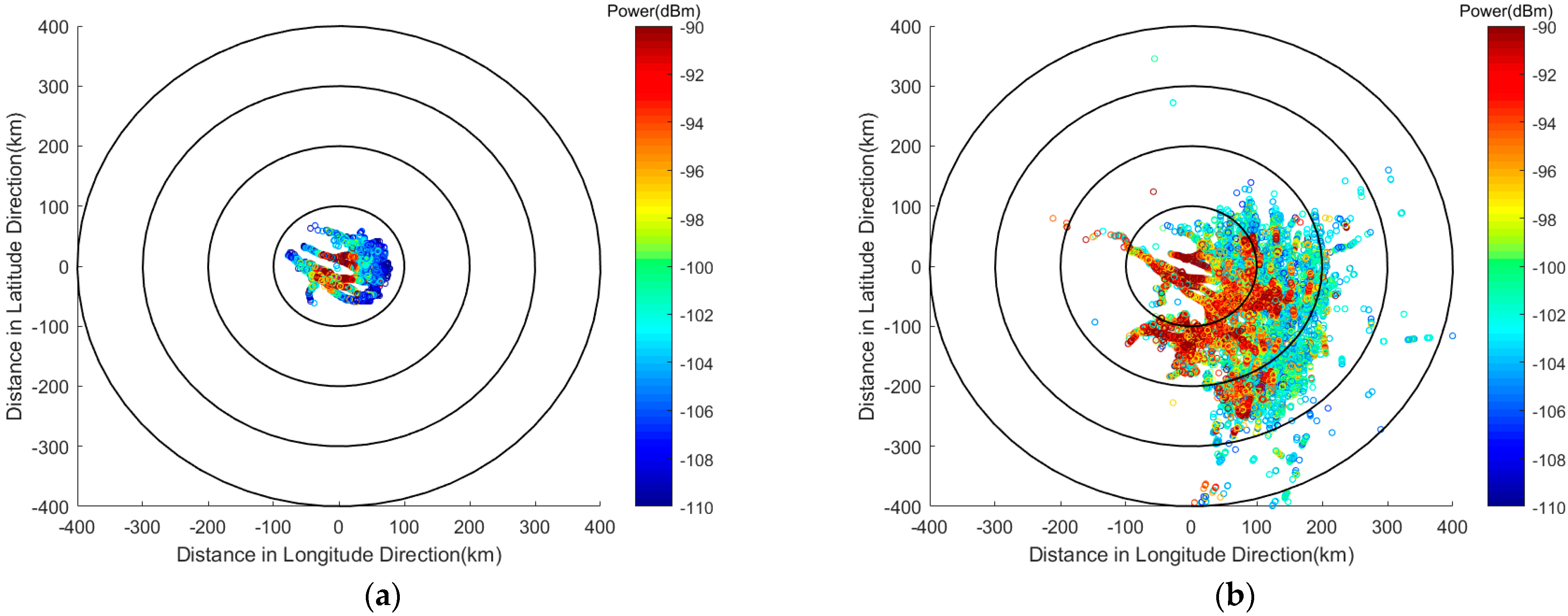
Figure 2.
Comparison diagram of AIS horizon signals and over-the-horizon signals. (a) AIS horizon signals; (b) AIS horizon and over-the-horizon signals.
Figure 2.
Comparison diagram of AIS horizon signals and over-the-horizon signals. (a) AIS horizon signals; (b) AIS horizon and over-the-horizon signals.
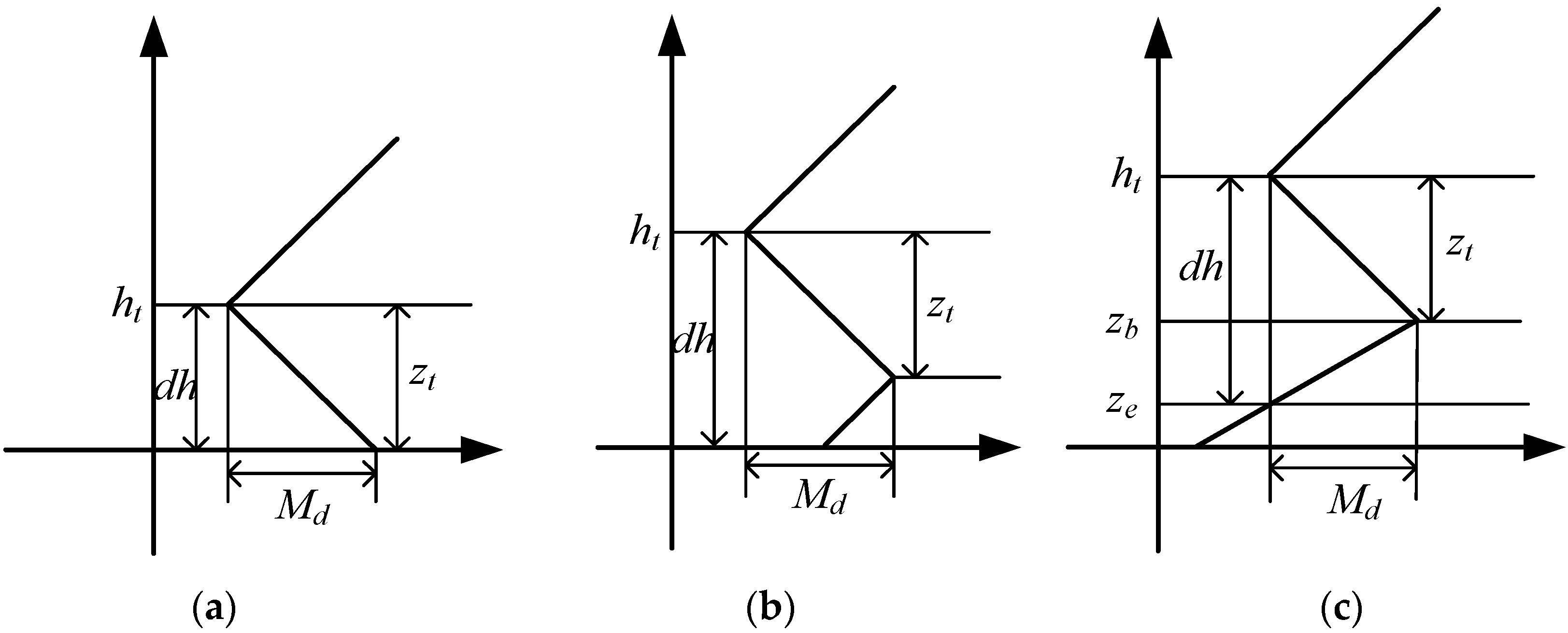
Figure 3.
Modified refractive index profiles of lower atmospheric duct. (a) Surface duct; (b) surface-based duct; (c) elevated duct.
Figure 3.
Modified refractive index profiles of lower atmospheric duct. (a) Surface duct; (b) surface-based duct; (c) elevated duct.
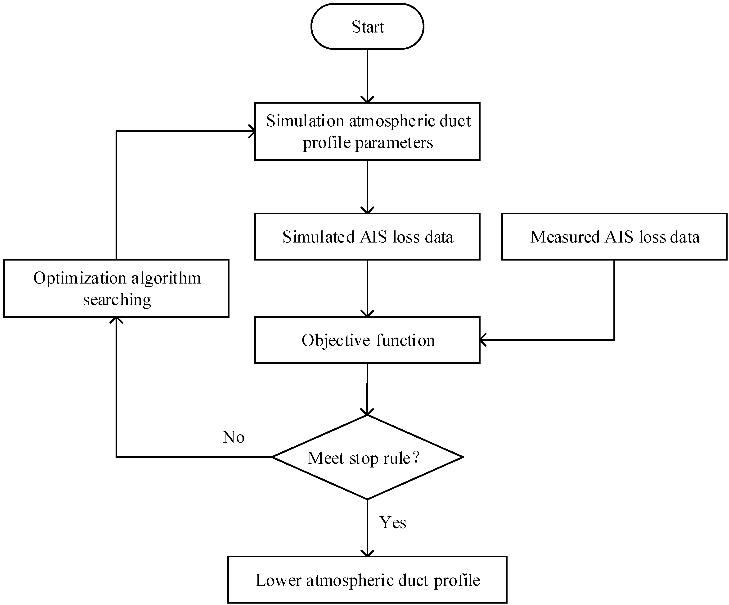
Figure 4.
AIS signal inversion for lower atmospheric duct.
Figure 4.
AIS signal inversion for lower atmospheric duct.
Figure 5.
Simulated atmospheric duct profile and path propagation loss. (a) Atmospheric duct profile; (b) path propagation loss of AIS signal.
Figure 5.
Simulated atmospheric duct profile and path propagation loss. (a) Atmospheric duct profile; (b) path propagation loss of AIS signal.
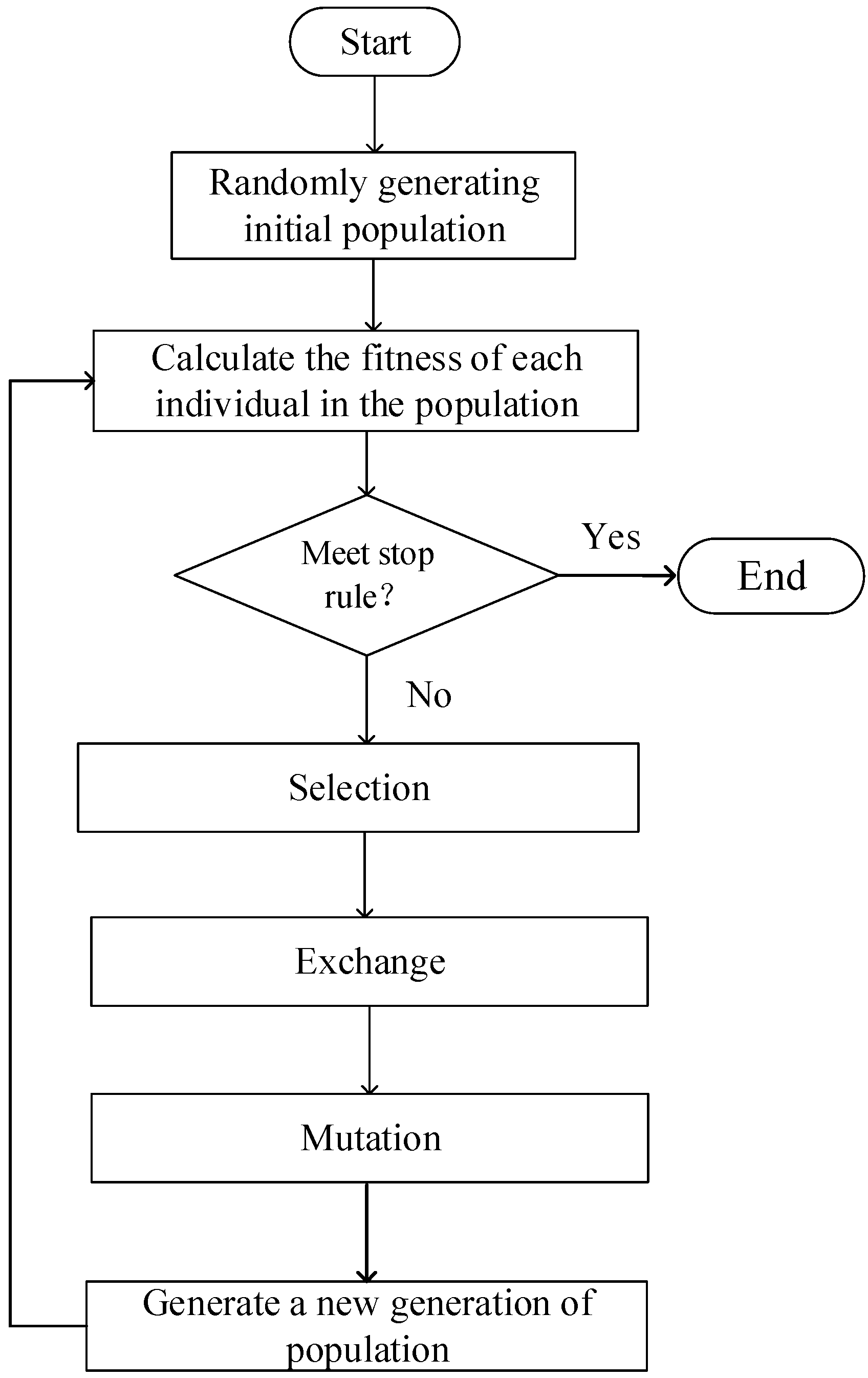
Figure 6.
Basic flowchart of GA.
Figure 6.
Basic flowchart of GA.
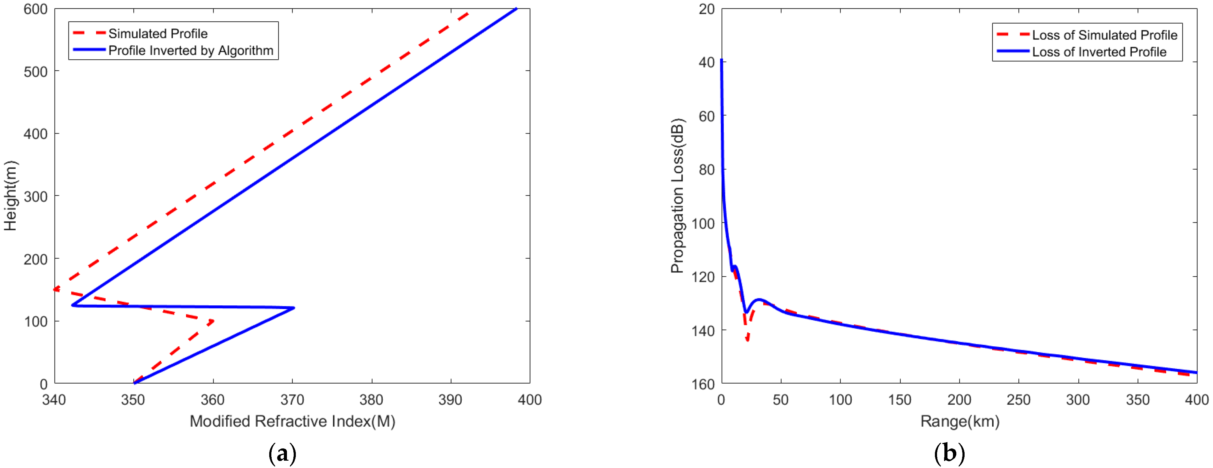
Figure 7.
GA inversion results. (a) Atmospheric duct profile; (b) path propagation loss of AIS signal.
Figure 7.
GA inversion results. (a) Atmospheric duct profile; (b) path propagation loss of AIS signal.
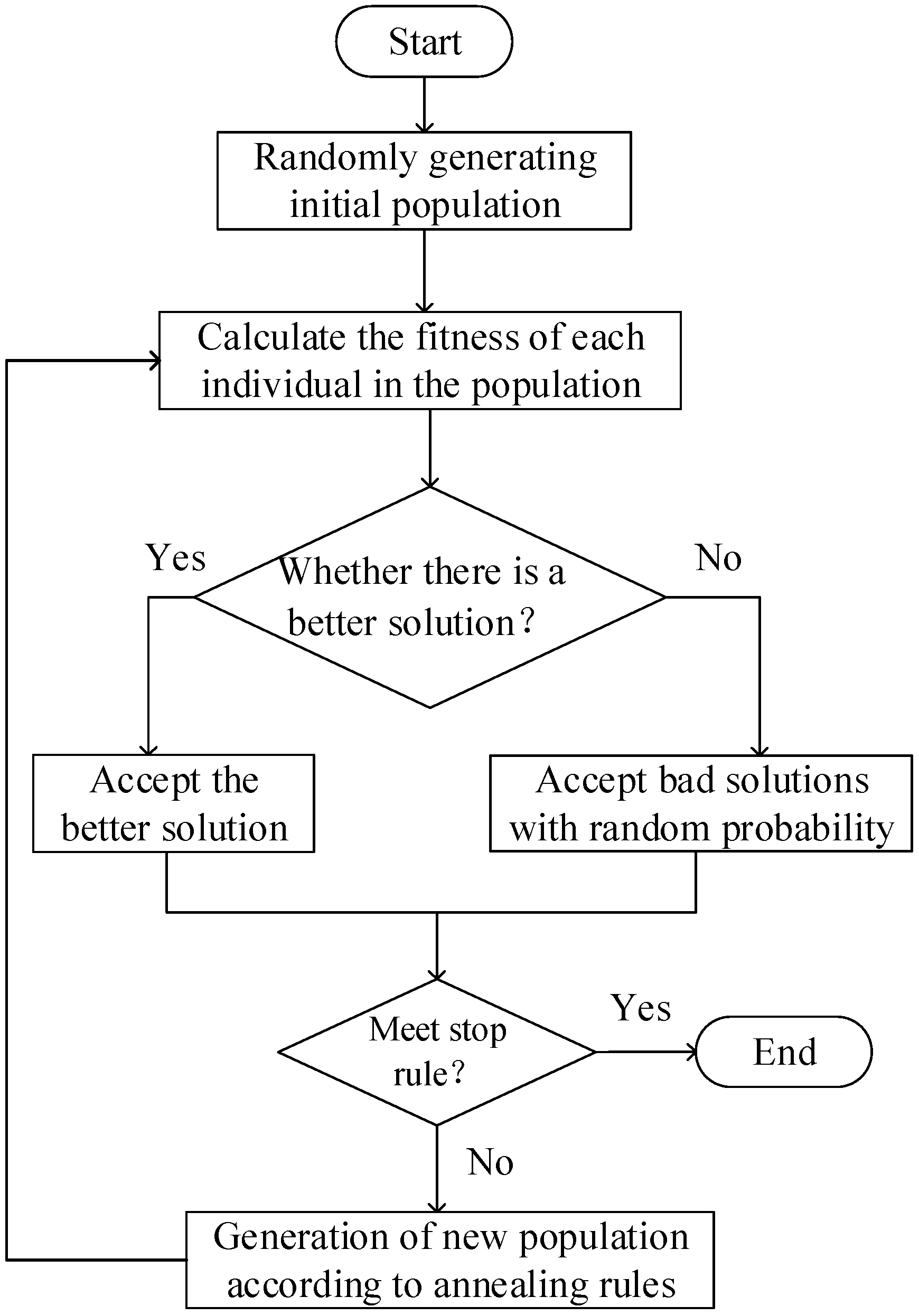
Figure 8.
Basic flowchart of SA algorithm.
Figure 8.
Basic flowchart of SA algorithm.
Figure 9.
SA algorithm inversion results. (a) Atmospheric duct profile; (b) path propagation loss of AIS signal.
Figure 9.
SA algorithm inversion results. (a) Atmospheric duct profile; (b) path propagation loss of AIS signal.
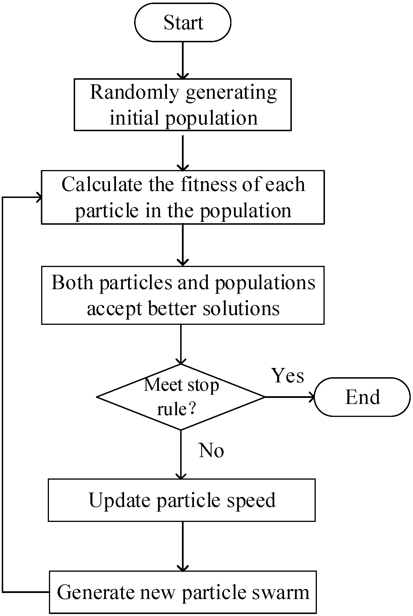
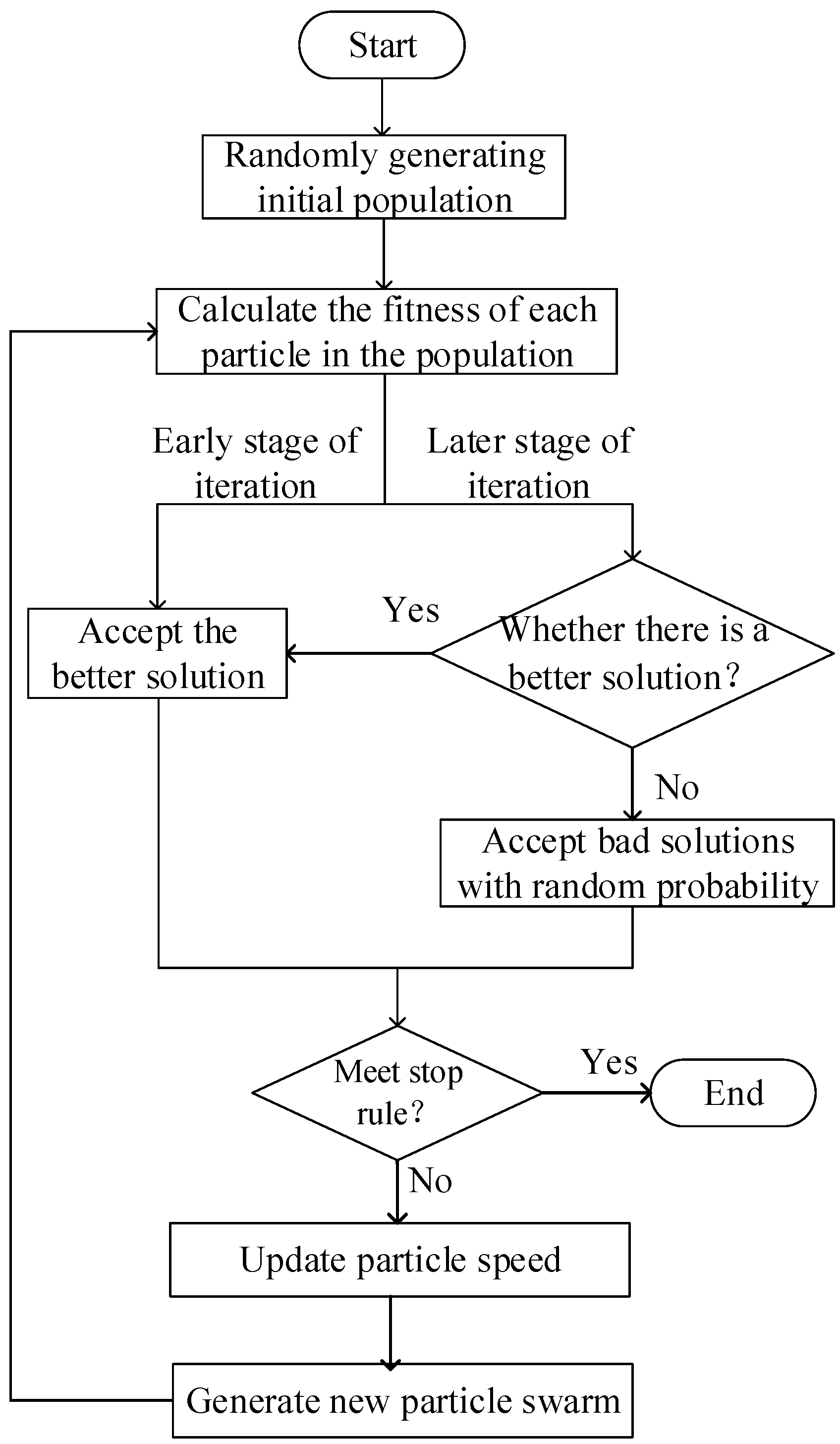
Figure 10.
Basic flowchart of PSO algorithm.
Figure 10.
Basic flowchart of PSO algorithm.
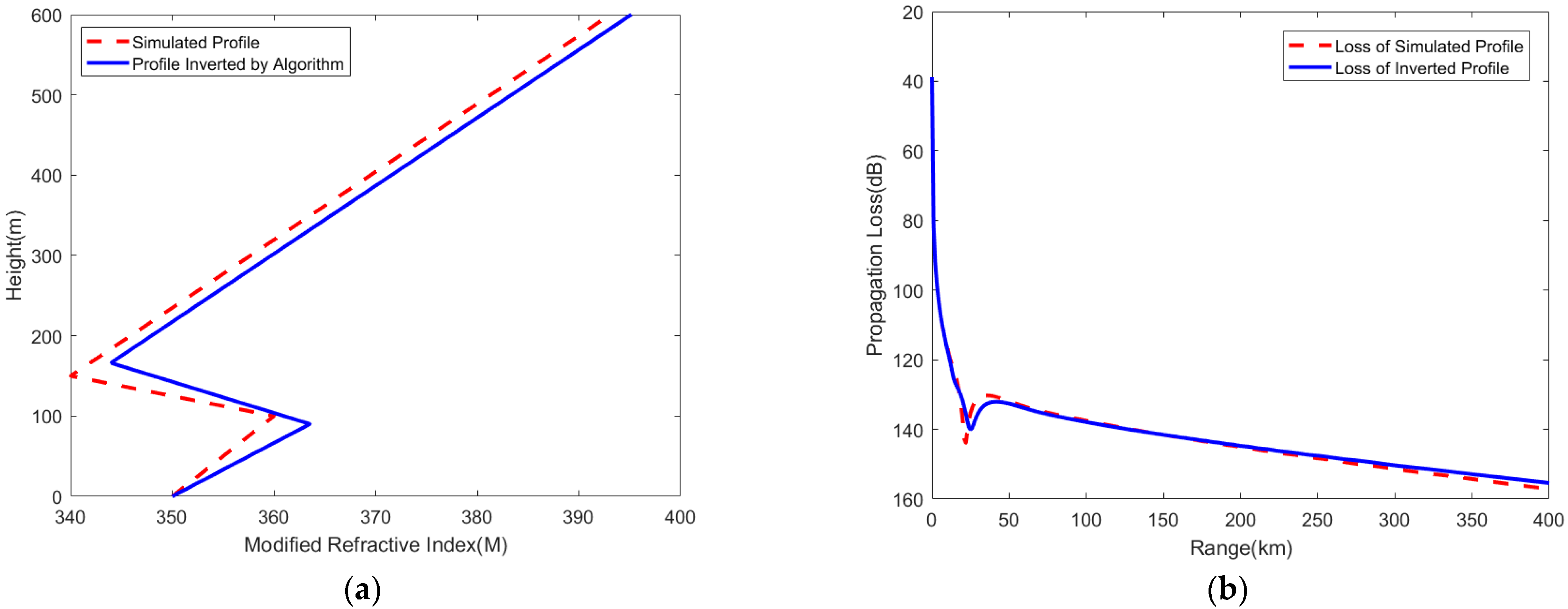
Figure 11.
PSO algorithm inversion results. (a) Atmospheric duct profile; (b) path propagation loss of AIS signal.
Figure 11.
PSO algorithm inversion results. (a) Atmospheric duct profile; (b) path propagation loss of AIS signal.
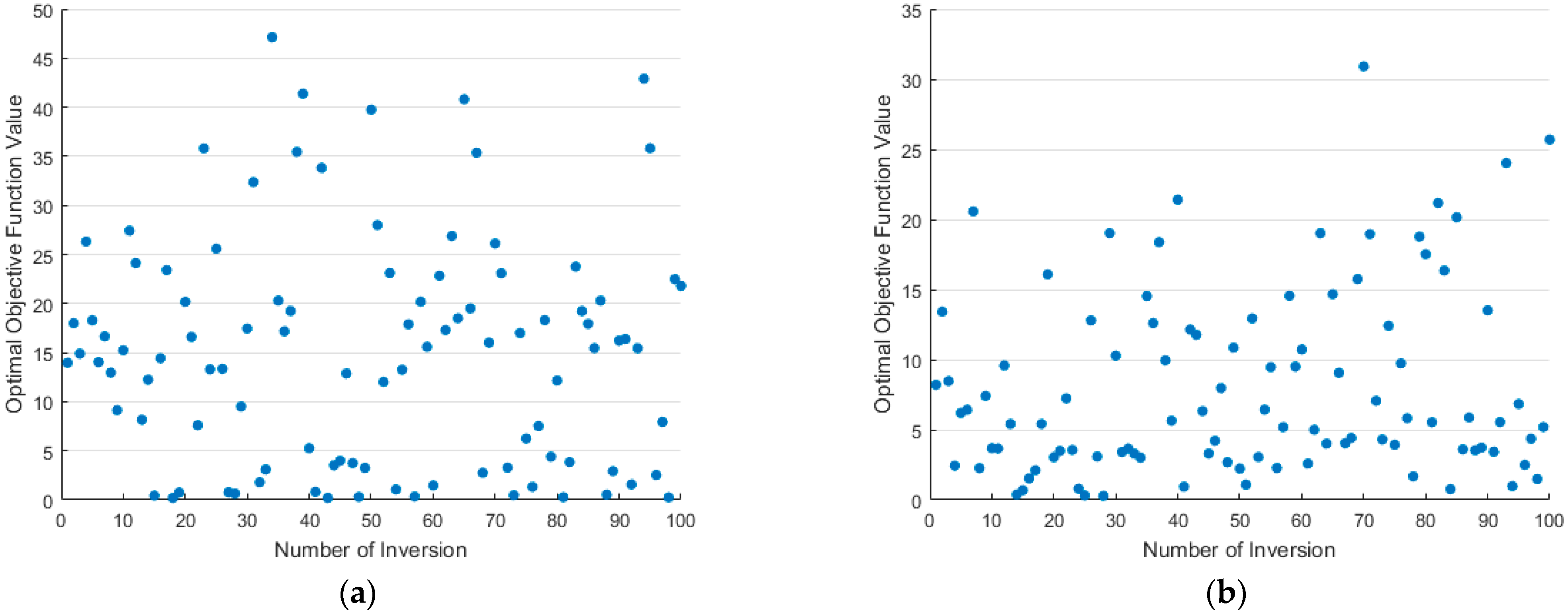
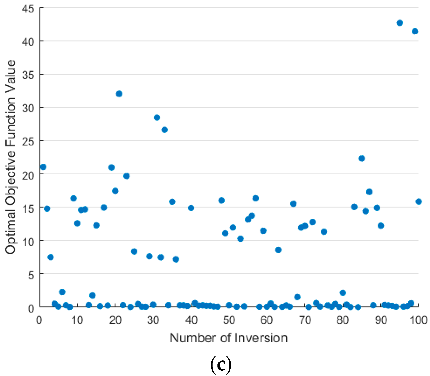
Figure 12.
Optimal objective function values obtained from inversion using three intelligent optimization algorithms. (a) GA; (b) SA algorithm; (c) PSO algorithm.
Figure 12.
Optimal objective function values obtained from inversion using three intelligent optimization algorithms. (a) GA; (b) SA algorithm; (c) PSO algorithm.
Figure 13.
Simulated elevated duct profile and path propagation loss. (a) Elevated duct profile; (b) path propagation loss of AIS signal.
Figure 13.
Simulated elevated duct profile and path propagation loss. (a) Elevated duct profile; (b) path propagation loss of AIS signal.
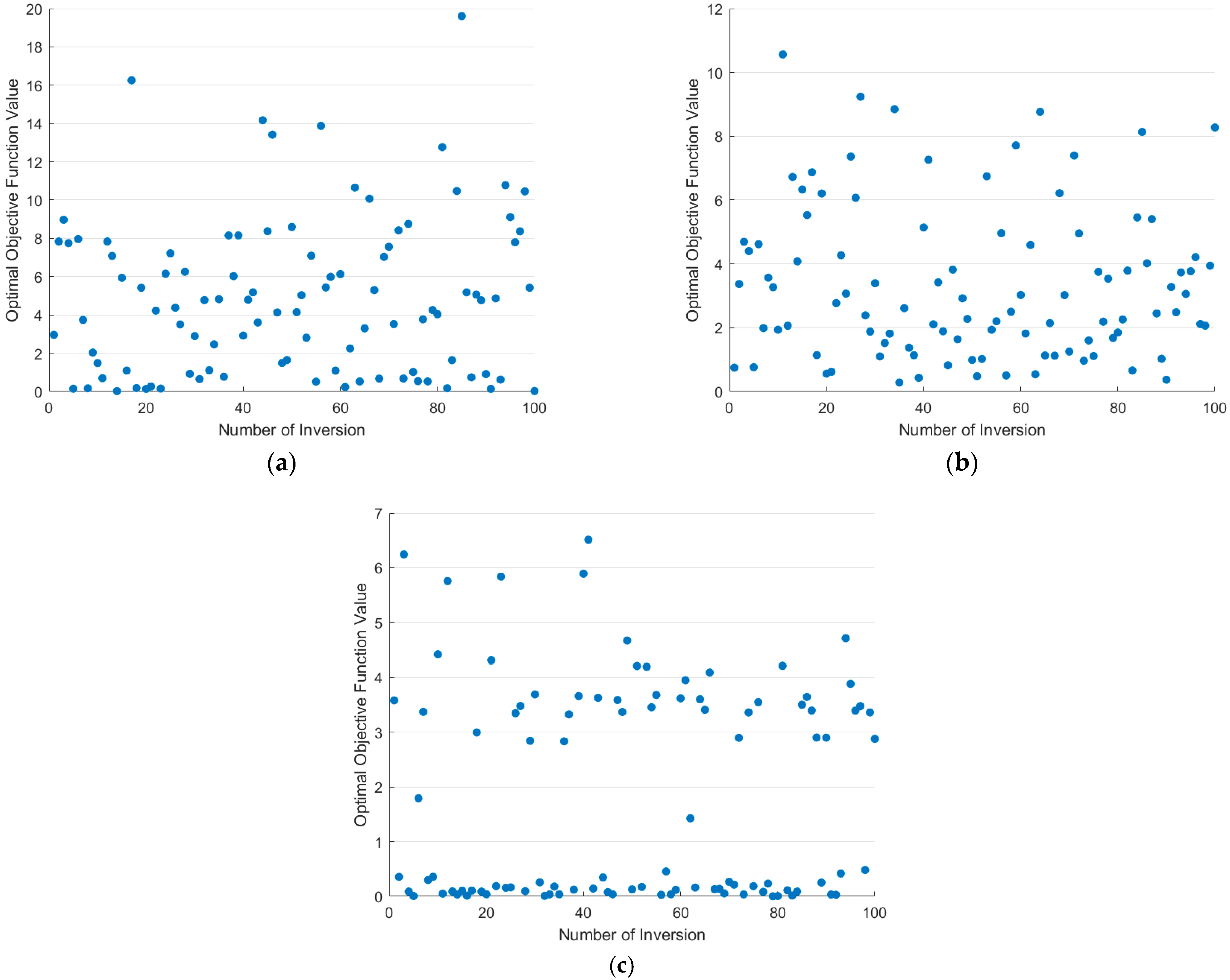
Figure 14.
Optimal objective function values obtained from inversion using three intelligent optimization algorithms. (a) GA; (b) SA algorithm; (c) PSO algorithm.
Figure 14.
Optimal objective function values obtained from inversion using three intelligent optimization algorithms. (a) GA; (b) SA algorithm; (c) PSO algorithm.
Figure 15.
Basic flowchart of the SAPSO algorithm.
Figure 15.
Basic flowchart of the SAPSO algorithm.
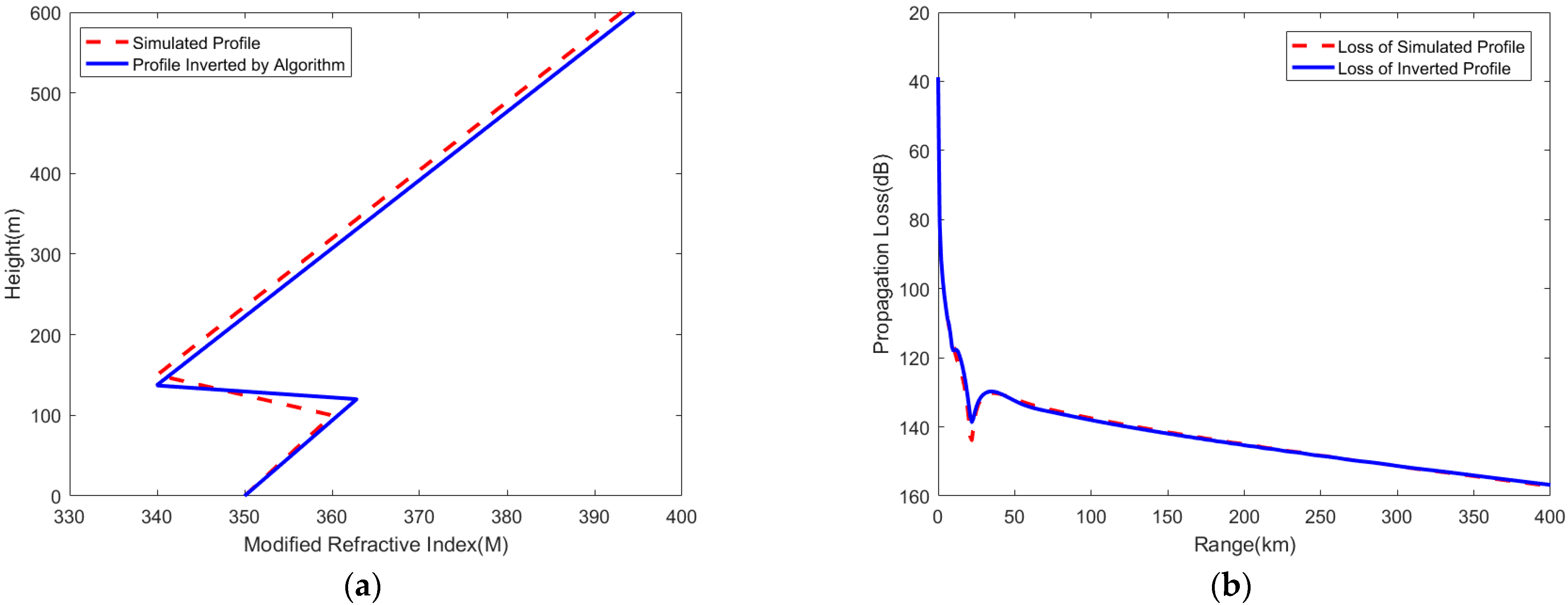
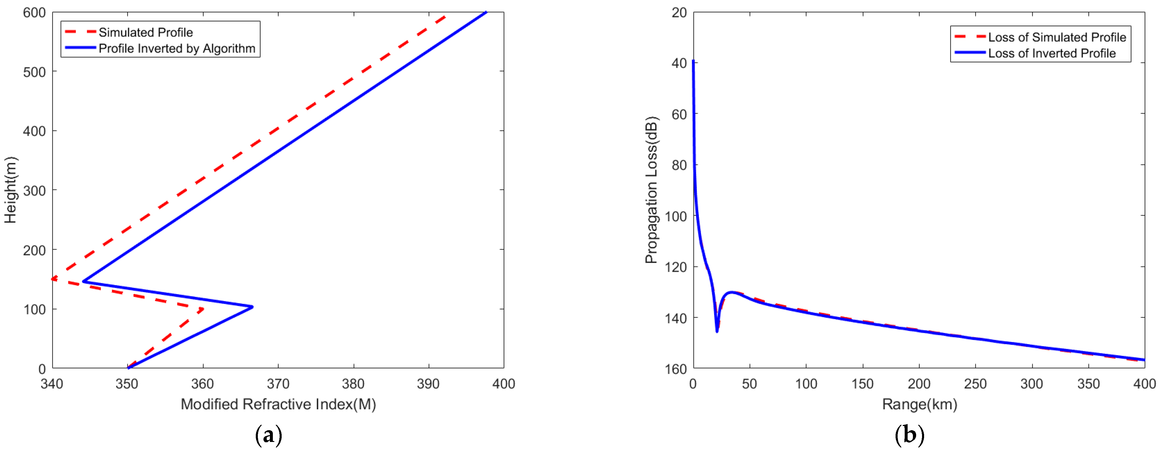
Figure 16.
SAPSO algorithm inversion results. (a) Atmospheric duct profile; (b) path propagation loss of AIS signal.
Figure 16.
SAPSO algorithm inversion results. (a) Atmospheric duct profile; (b) path propagation loss of AIS signal.
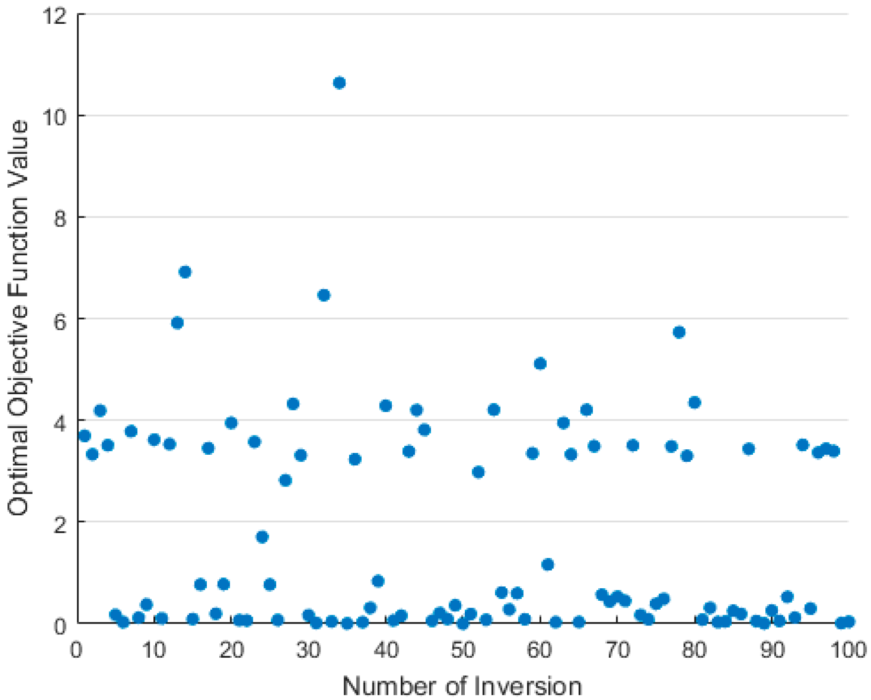
Figure 17.
Optimal objective function values of SAPSO algorithm inversion.
Figure 17.
Optimal objective function values of SAPSO algorithm inversion.
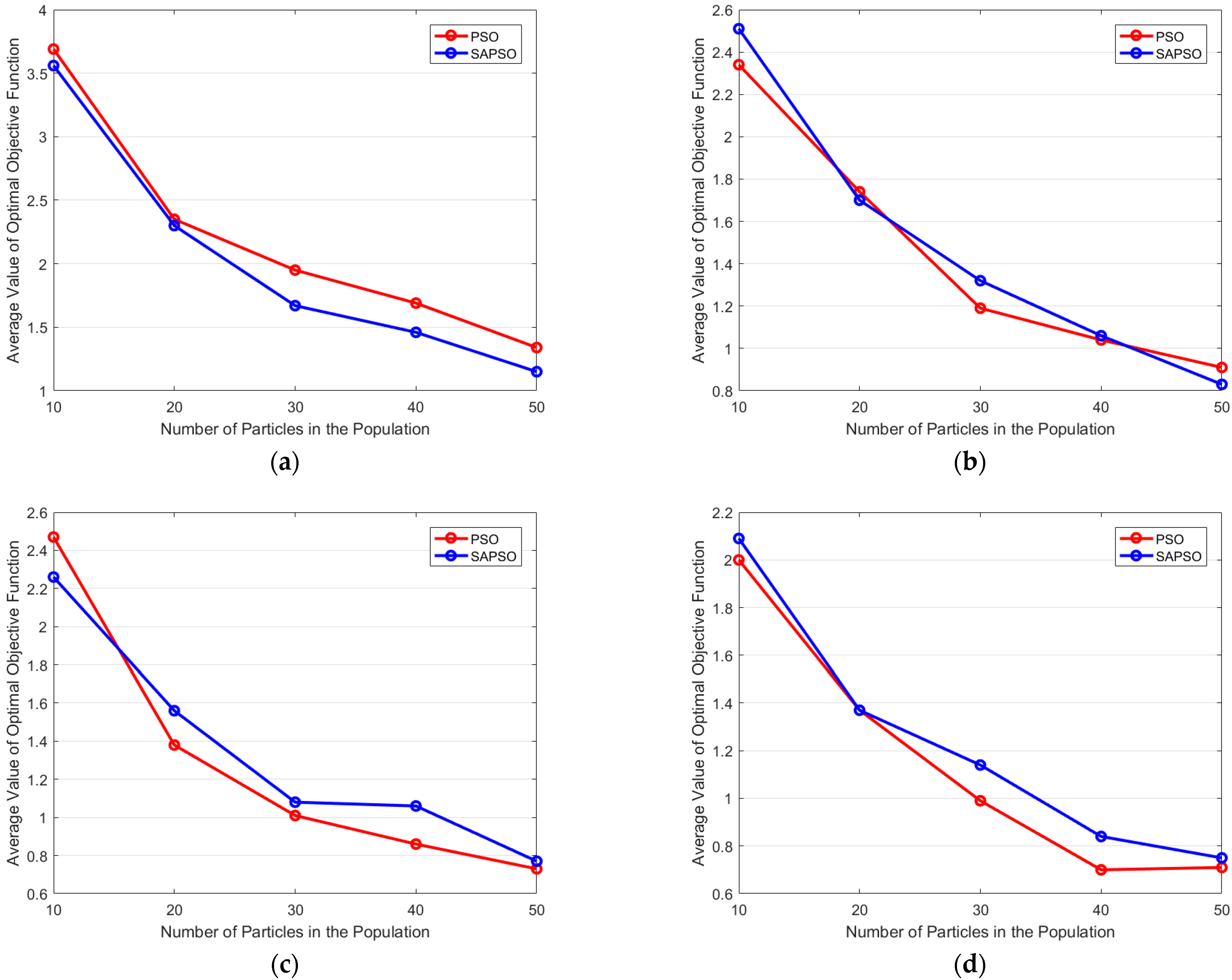
Figure 18.
Comparison of PSO and SAPSO inversion results under different numbers of iterations. (a) 10; (b) 20; (c) 30; and (d) 40 iterations.
Figure 18.
Comparison of PSO and SAPSO inversion results under different numbers of iterations. (a) 10; (b) 20; (c) 30; and (d) 40 iterations.
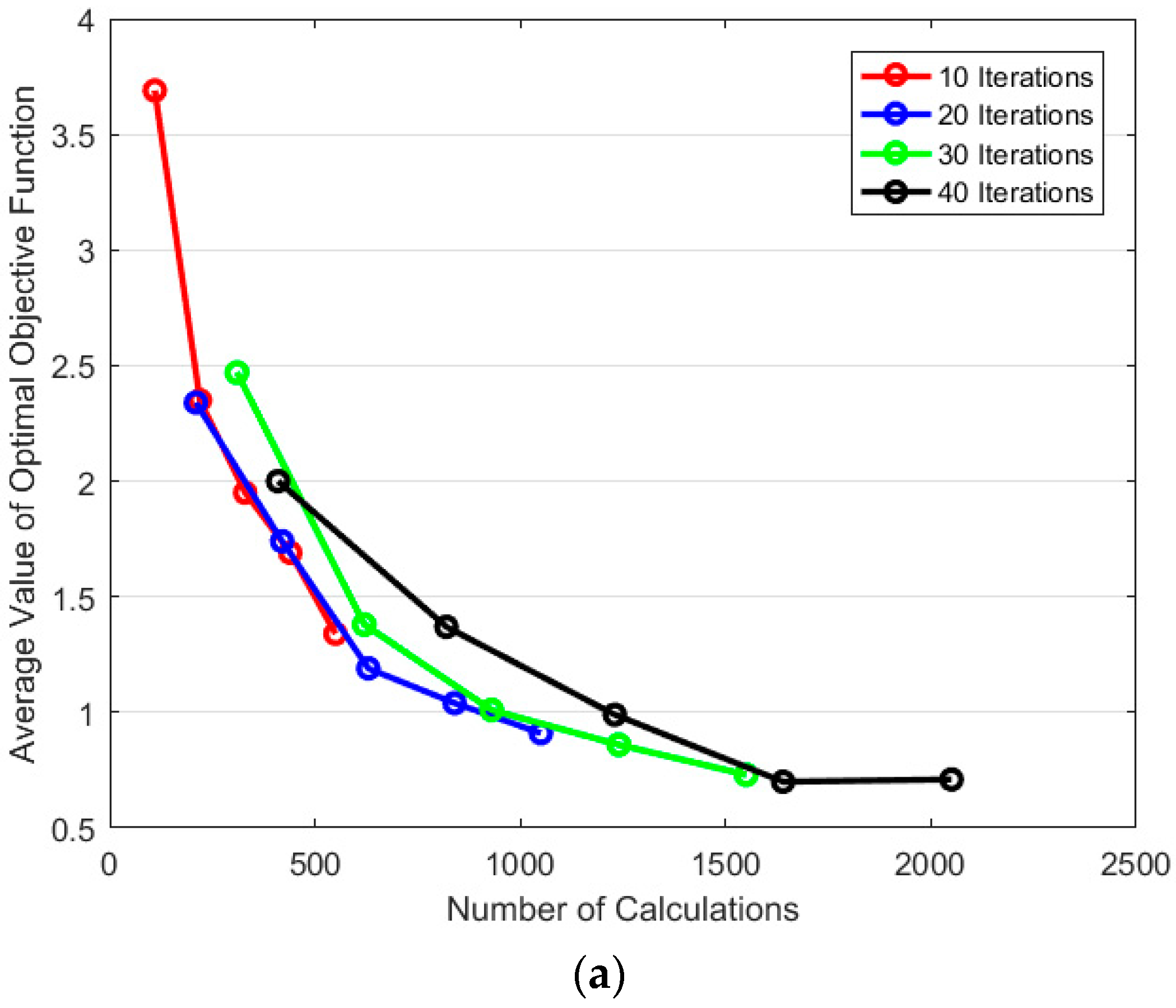
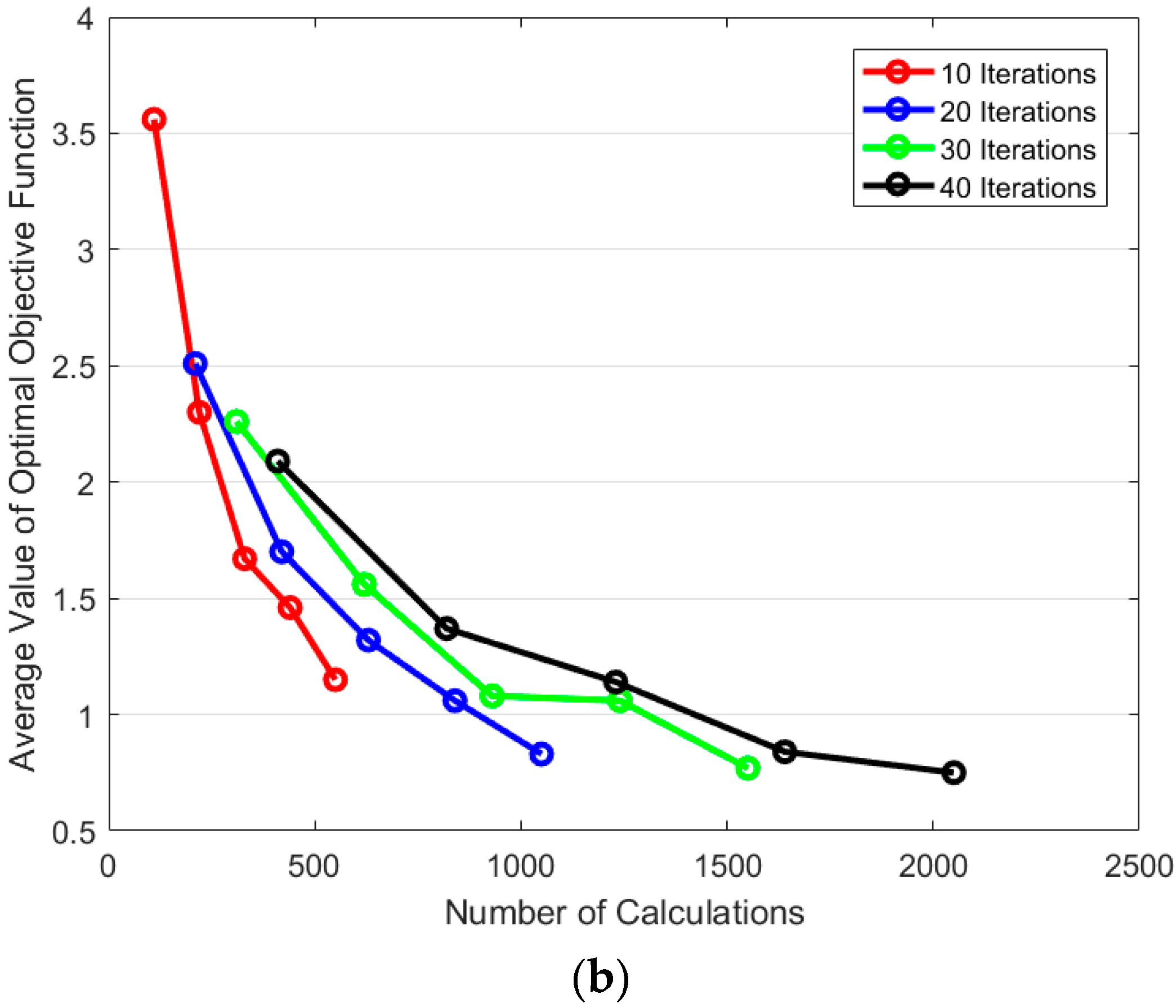
Figure 19.
Inversion results under different numbers of calculations. (a) PSO algorithm; (b) SAPSO algorithm.
Figure 19.
Inversion results under different numbers of calculations. (a) PSO algorithm; (b) SAPSO algorithm.
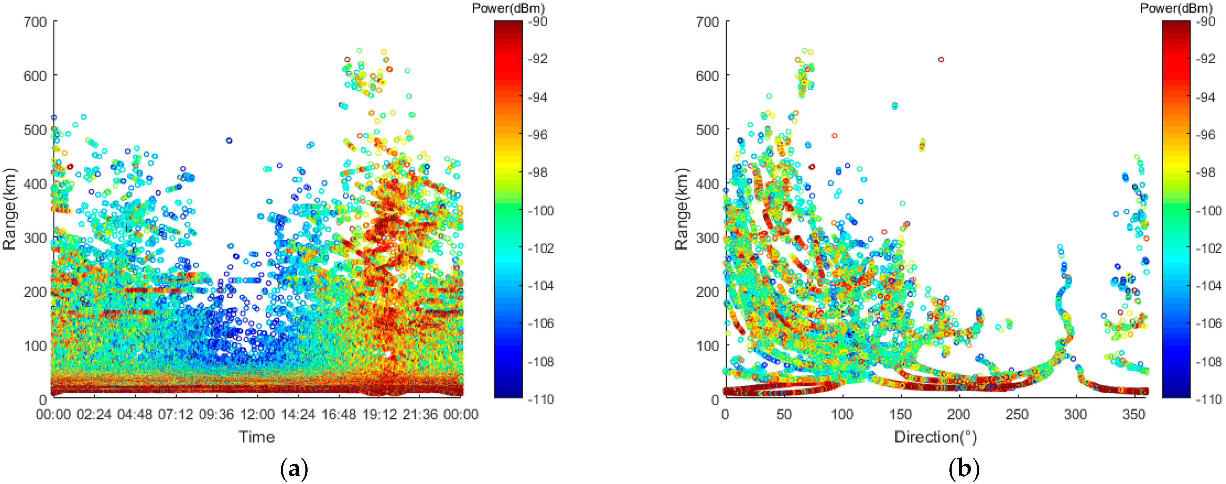
Figure 20.
Measured AIS signal power data from 4 October 2021. (a) Distance−time distribution; (b) distance−azimuth distribution.
Figure 20.
Measured AIS signal power data from 4 October 2021. (a) Distance−time distribution; (b) distance−azimuth distribution.
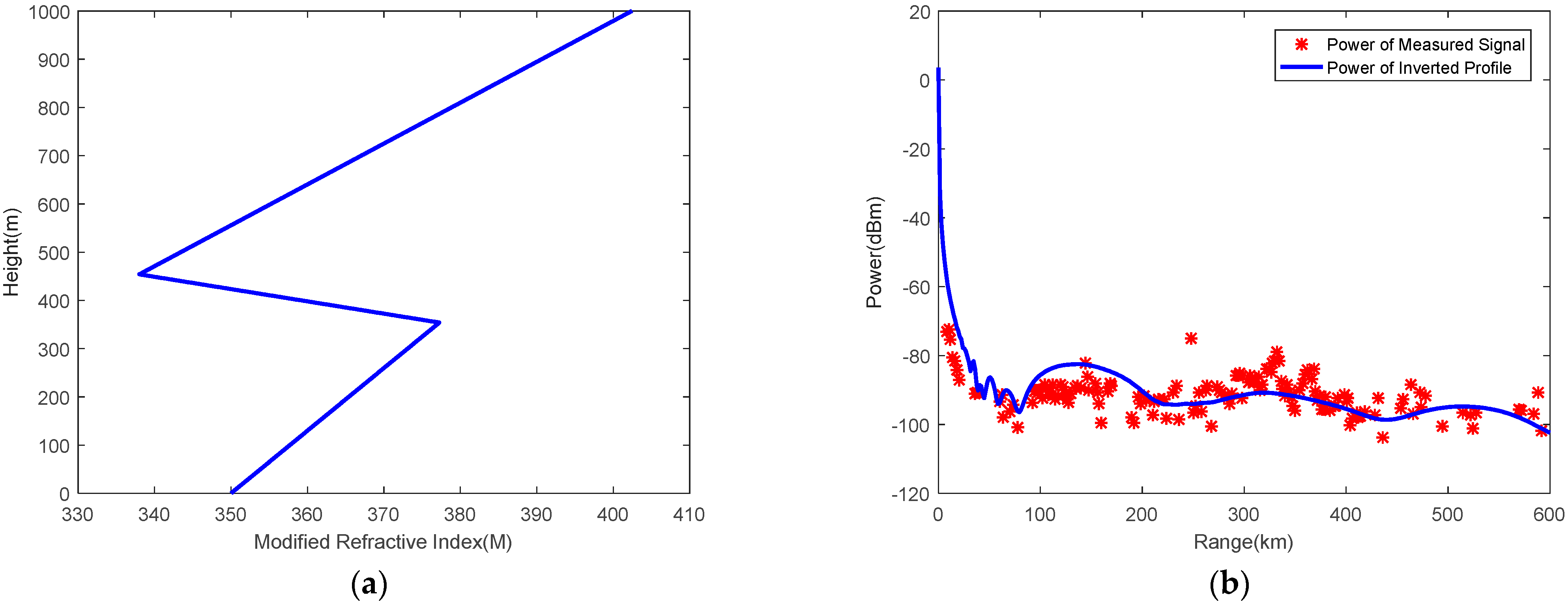
Figure 21.
Inversion results using AIS measured data at 19:00 and 60°. (a) Inverted atmospheric duct profile; (b) comparison of measured signal power and inverted profile calculation power.
Figure 21.
Inversion results using AIS measured data at 19:00 and 60°. (a) Inverted atmospheric duct profile; (b) comparison of measured signal power and inverted profile calculation power.
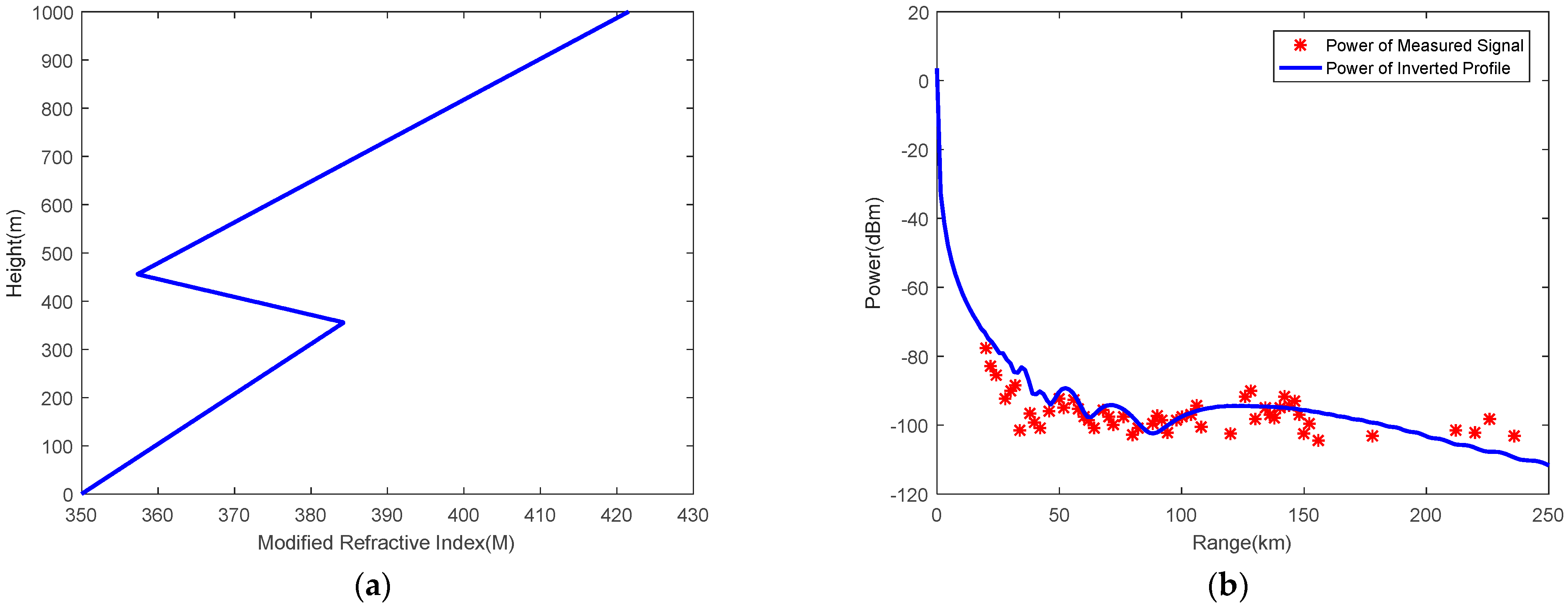
Figure 22.
Inversion results using AIS measured data at 5:00 and 290°. (a) Inverted atmospheric duct profile; (b) comparison of measured signal power and inverted profile calculation power.
Figure 22.
Inversion results using AIS measured data at 5:00 and 290°. (a) Inverted atmospheric duct profile; (b) comparison of measured signal power and inverted profile calculation power.
Table 1.
Simulated lower atmospheric duct profile parameters.
Table 1.
Simulated lower atmospheric duct profile parameters.
| Parameter | Value |
|---|
| Slope of bottom layer (c) | 0.1 M unit/m |
| Bottom height of duct layer () | 100 m |
| Thickness of duct layer () | 50 m |
| Duct strength (Md) | 20 M unit |
Table 2.
Limits of lower atmospheric duct parameters.
Table 2.
Limits of lower atmospheric duct parameters.
| Parameter | Minimum | Maximum |
|---|
| c (M Unit/m) | 0 | 0.2 |
| (m) | 0 | 400 |
| (m) | 1 | 100 |
| Md (M Unit) | 1 | 80 |
Table 3.
Parameters of GA.
Table 3.
Parameters of GA.
| Parameter | Value |
|---|
| Genetic algebra | 20 |
| Population size | 20 |
| Generation gap | 0.95 |
| Exchange rate | 0.7 |
| Mutation rate | 0.01 |
Table 4.
Lower atmospheric duct parameters retrieved by GA.
Table 4.
Lower atmospheric duct parameters retrieved by GA.
| Parameter | Simulated True Value | Inverted Value |
|---|
| c (M Unit/m) | 0.1 | 0.167 |
| (m) | 100 | 121.7 |
| (m) | 50 | 2.3 |
| Md (M Unit) | 20 | 28.2 |
Table 5.
Parameters of SA algorithm.
Table 5.
Parameters of SA algorithm.
| Parameter | Value |
|---|
| Maximum number of iterations | 20 |
| Iterations per temperature | 20 |
| Initial temperature | 100 |
| Temperature attenuation coefficient | 0.95 |
Table 6.
Lower atmospheric duct parameters retrieved by SA algorithm.
Table 6.
Lower atmospheric duct parameters retrieved by SA algorithm.
| Parameter | Simulated True Value | Inverted Value |
|---|
| c (M Unit/m) | 0.1 | 0.15 |
| (m) | 100 | 90.1 |
| (m) | 50 | 76.1 |
| Md (M Unit) | 20 | 19.6 |
Table 7.
Parameters of PSO algorithm.
Table 7.
Parameters of PSO algorithm.
| Parameter | Value |
|---|
| Maximum number of iterations | 20 |
| Number of particles | 20 |
| Individual learning factor | 2 |
| Social learning factor | 2 |
| Maximum inertia factor | 0.9 |
| Minimum inertia factor | 0.4 |
Table 8.
Lower atmospheric duct parameters retrieved by PSO algorithm.
Table 8.
Lower atmospheric duct parameters retrieved by PSO algorithm.
| Parameter | Simulated True Value | Inverted Value |
|---|
| c (M Unit/m) | 0.1 | 0.11 |
| (m) | 100 | 120.1 |
| (m) | 50 | 17.0 |
| Md (M Unit) | 20 | 22.9 |
Table 9.
Simulated elevated duct profile parameters.
Table 9.
Simulated elevated duct profile parameters.
| Parameter | Value |
|---|
| Slope of bottom layer (c) | 0.15 M unit/m |
| Bottom height of duct layer () | 80 m |
| Thickness of duct layer () | 60 m |
| Duct strength (Md) | 8 M unit |
Table 10.
Parameters of SAPSO algorithm.
Table 10.
Parameters of SAPSO algorithm.
| Parameter | Value |
|---|
| Maximum number of iterations | 20 |
| Number of particles | 20 |
| Individual learning factor | 2 |
| Social learning factor | 2 |
| Maximum inertia factor | 0.9 |
| Minimum inertia factor | 0.4 |
| Initial temperature | 100 |
| Temperature attenuation coefficient | 0.95 |
Table 11.
Lower atmospheric duct parameters retrieved by SAPSO algorithm.
Table 11.
Lower atmospheric duct parameters retrieved by SAPSO algorithm.
| Parameter | Simulated True Value | Inverted Value |
|---|
| c (M Unit/m) | 0.1 | 0.16 |
| (m) | 100 | 103.7 |
| (m) | 50 | 42.0 |
| Md (M Unit) | 20 | 22.6 |
Table 12.
Average of optimal objective function values under different inversion parameters.
Table 12.
Average of optimal objective function values under different inversion parameters.
| Population Size | Number of Iterations for PSO | Number of Iterations for SAPSO |
|---|
| 10 | 20 | 30 | 40 | 10 | 20 | 30 | 40 |
|---|
| 10 | 3.69 | 2.34 | 2.47 | 2 | 3.56 | 2.51 | 2.26 | 2.09 |
| 20 | 2.35 | 1.74 | 1.38 | 1.37 | 2.3 | 1.7 | 1.56 | 1.37 |
| 30 | 1.95 | 1.19 | 1.01 | 0.99 | 1.67 | 1.32 | 1.08 | 1.14 |
| 40 | 1.69 | 1.04 | 0.86 | 0.7 | 1.46 | 1.06 | 1.06 | 0.84 |
| 50 | 1.34 | 0.91 | 0.73 | 0.71 | 1.15 | 0.83 | 0.77 | 0.75 |
Table 13.
Selected parameters for inversion using measured AIS data.
Table 13.
Selected parameters for inversion using measured AIS data.
| Parameter | Value |
|---|
| Inversion algorithm | SAPSO |
| Maximum number of iterations | 10 |
| Number of particles | 50 |
| Individual learning factor | 2 |
| Social learning factor | 2 |
| Maximum inertia factor | 0.9 |
| Minimum inertia factor | 0.4 |
| Initial temperature | 100 |
| Temperature attenuation coefficient | 0.95 |


 ,
, 


