Development of AI- and Robotics-Assisted Automated Pavement-Crack-Evaluation System

Abstract

Crack inspection is important to monitor the structural health of pavement structures and make the repair process easier. Currently, pavement crack inspection is conducted manually, which is inefficient and costly at the same time. To solve the problem, this work has developed a robotic system for automated data collection and analysis in real-time. The robotic system navigates the pavement and collects visual images from the surface. A deep-learning-based semantic segmentation framework named RCDNet was proposed. The RCDNet was implemented on the onboard computer of the robot to identify cracks from the visual images. The encoder-decoder architecture was utilized as the base framework of the proposed RCDNet. The RCDNet comprises a dual-channel encoder and a decoder module. The encoder and decoder parts contain a context-embedded channel attention (CECA) module and a global attention module (GAM), respectively. Simulation results show that the deep learning model obtained 96.29% accuracy for predicting the images. The proposed robotic system was tested in both indoor and outdoor environments. The robot was observed to complete the inspection of a 3 m × 2 m grid within 10 min and a 2.5 m × 1 m grid within 6 min. This outcome shows that the proposed robotic method can drastically reduce the time of manual inspection. Furthermore, a severity map was generated using the visual image results. This map highlights areas that require greater attention for repair in the test grid.

1. Introduction

Roads in South Korea have a length of 105,673 Km, of which 89,701 are paved roads (91.6%) [1]. These paved roads can be damaged for various reasons, including surface cracking, delamination, honeycomb, etc. Cracks in paved roads are one of the most potent indicators of pavement damage. Cracking in the pavement is quite unavoidable, and there are many underlying factors (e.g., exposure to the sun, rain erosion, natural weathering, and long-term driving of vehicles) that accelerate the cracking of the pavement’s surface. If these cracks cannot be localized and repaired in time, they will have a negative impact on the safe driving of vehicles. Consequently, it can cause deadly accidents, as well as expenditure of a huge amount of money for the maintenance and repair of pavements. Therefore, crack detection at an early stage is essential to maintain the structural integrity and serviceability of paved roads. In past decades, manual crack detection was a very common practice for localizing cracks on paved roads. However, the manual method lacks efficiency and accuracy; it is expensive because of the necessary expertise. Moreover, it is considerably tedious, arduous, and time-consuming because experts must monitor the cracks with the naked eye by roaming the roads. Therefore, to lessen the workload of experts and make the system fast and cost-effective, researchers are bringing automation to crack detection. With the advancement of computer vision (CV) technology, various vision-based methodologies have already been developed to perform automatic crack detection. Early implementation of the CV techniques for crack detection was to some extent limited to threshold-based approaches (e.g., pixel intensity was used as the feature) [2,3], and other hand-crafted feature-based approaches. Some of the prominent hand-crafted feature-extraction techniques are wavelet features [4], Local Binary Pattern (LBP) [5], Digital Image Co-relation [6], Gabor filters [7], and so on. But these methods can only extract local patterns instead of global patterns, which pulls the detection results backward. Some research [8,9,10] has used model-based, traditional CV algorithms, which use geometric characteristics of images to perform crack detection globally. The advantages of model-based techniques over feature-based techniques are that model-based techniques can detect cracks in adverse conditions such as noisy environments, poor illumination conditions, and shadow problems. Though these model-based methods can partially solve noise problems and can detect cracks more continuously, their performance is not satisfactory enough when detecting cracks with complex patterns or intensity inhomogeneity.

In recent years, Deep Learning has been extensively applied in CV tasks for its noteworthy representation ability. DL models do not need hand-crafted features; rather, they can extract valuable features (both local and global) automatically from the input data. A few research works have already devoted their efforts to utilizing the properties of deep learning mentioned above to learn robust feature representation and detect cracks with more precision. Zhang et al. introduced a Convolutional Neural Network (CNN) classifier for the first time in 2016 to detect cracks in concrete structures [11]. The primary objective of this study was to develop a patch-based classifier to detect cracks in concrete structures. Later on, Cha et al. [12] and Eisenbach et al. [13] also performed patch-based classification, which can only identify the presence or absence of cracks in a corresponding image patch. Researchers also utilized another deep learning scheme called object detection for localizing the cracks, along with identifying them in an image [14,15]. However, these models can only classify and localize the cracks in a concrete structure instead of detecting cracks at a pixel level. So to solve this issue, Yang et al. incorporated an image segmentation technique for detecting concrete cracks at pixel level [16]. Crack segmentation involves classifying each of the pixels in an image as ’crack’ or ’non-crack’. Instead of detecting the class only in an image, crack segmentation detects an output image, highlighting the pixels containing the cracks, which localizes the cracks and extracts the original shape of the cracks. Moreover, the segmented images can later be used for the important task of extracting length, width, and area of cracks, which provides information about crack severity in concrete structures. Considering the advantages of crack segmentation over crack detection and classification, researchers from all over the world are devoting their efforts to developing crack-segmentation methods and quantifying the cracks to present an automated crack-detection system [17,18].

However, along with the automated detection of cracks, automatic data collection is also necessary for developing a fully automated pavement inspection system. While automated crack detection increases accuracy, automated data collection can save time and also handle safety issues. As a whole, many researchers have already utilized robotic vehicles as well as unmanned aerial vehicles to collect the images automatically [19,20]. However, most researchers collect the data with their vehicle and transfer them to another computer for analysis, which cannot be considered a real-time detection method for saving time. So, considering the above-mentioned issues, this work develops a robotic-assisted pavement inspection system that collects image data automatically and detects cracks from images in real time using our proposed deep learning models. Furthermore, after generating the images, this work will quantify the cracks to present severity maps of the cracks. This work will solve the problems of manual crack detection techniques through our proposed system. The automatic data collection saves time and also handles safety issues. The detection using our proposed deep learning model increases the accuracy, and finally, as this work is proposing a totally automated pavement inspection system, it will not need experts’ involvement, which will reduce the expenses as well. This work thereby develops a robotic-assisted pavement-inspection system. The main contributions of this study are as follows.

• Developing a robotics platform that will collect visual data automatically;
• Presenting a novel deep learning model to implement the platform on the robot’s onboard computer to detect cracks from the RGB images in real-time;
• Presenting a crack quantification algorithm for finding out crack length, width, and area;
• Finally, presenting a visualization of the crack severity map.

The rest of this research is organized as follows: Section 2 provides an overview of the existing research works that focus on developing robotic vehicles for pavement inspection. Section 3 presents the architecture of the robotic platform used in this work. Section 4 presents the crack segmentation technique from RGB images. Section 5 presents the working principle of the robotic platform. Section 6 discusses the experimental procedure and shows the obtained result of our proposed system. Section 7 discusses the drawbacks of the proposed system. This work is concluded in Section 8. Our code is public at https://github.com/Masrur02/AMSEL_robot (accessed on 16 July 2023).

2. Literature Review

In this section, this paper will briefly summarize the existing state-of-the-art related research that focuses on developing robotic-assisted systems for inspecting cracks in concrete structures in real-time.

2.1. Robotic System for Crack Inspection

2.1.1. Traditional Methods

In past decades, various researchers have developed robotic vehicles to automatically inspect cracks. The first study, dating back to 2007 [19], designed an automated inspection system for cracks in concrete tunnels using a mobile robot. They collected the images using a CCD camera, which was interfaced with the robot, and stored the images in the robot’s brain. Later, they extracted cracks on a different computer using the Sobel edge-detection algorithm. Oyekola et al. also designed a robotic system for detecting cracks on concrete tank surfaces [21]. The authors also first collected the images and later detected cracks using a thresholding algorithm developed using the MATLAB programming language. Li et al. utilized the robotic platform developed by Guimu Robot Co Ltd., Shanghai, China for detecting cracks on pavement structures [22]. The authors developed an unsupervised algorithm named the Multiscale Fusion Crack Detection (MFCD) for inspecting the cracks. However, in this research, the cracks are also not detected by the onboard computer. La et al. developed a wall-climbing robot for detecting cracks on steel bridges [23]. The robot was equipped with several sensors and a camera. Navigating through the steel bridges, it collected data and passed them in real-time to the ground station for further processing and for detecting cracks using a Hessian-matrix-based filter. In another work, La et al. used the Seekur mobile robot platform and modified it by installing several NDE sensors (e.g., GPR, USW, ER, IE) and a camera for the monitoring of a concrete bridge deck [24]. The authors collected the images and passed them to the remote computer to extract the cracks using a Gradient-based algorithm. They also presented the delamination maps of the cracking using NDE data. The robot could localize itself and maneuver automatically on the bridge deck. However, this robotic system needed multiple onboard computers for navigating and processing everything. In the studies [19,21,22,23,24], the researchers relied on conventional methods for crack assessment, employing image-processing algorithms and threshold-based approaches. While these methods provided initial insights, their weaknesses lie in accurate detection as well as in the lack of post-processing techniques to obtain comprehensive geometric information about the cracks. Additionally, the reliance on external computers for crack detection introduced potential delays and limitations in real-time assessment.

2.1.2. Learning-Based Methods

Hendrik et al. developed a legged robot named ANYmal for inspecting the crack conditions in underground tunnels [25]. The researchers considered the tactile sensory system instead of the vision data because of the presence of noise, water, etc., on the surface. They collected signals from the footsteps of the robot and classified the crack conditions using the Support Vector Machine (SVM) algorithm. The authors classified five types of crack conditions, including good, satisfactory, fair, critical, and failure, to provide information about the severity. Le et al. developed a mobile robotic system for the in-line inspection of the pipes [26]. The authors integrated multiple sensors (e.g., LIDAR, optic sensors) on the robot and classified these combined sensory data using the SVM algorithm for detecting cracks in pipes. Lei et al. developed a low-cost unmanned aerial vehicle for inspecting cracks in concrete structures [20]. They collected images using their UAV and classified cracks using the SVM classifier running on the onboard computer. Pan et al. utilized low-altitude images collected from a UAV to detect cracks on asphalt pavements [27]. The researchers collected centimeter-level spatial resolution images and utilized a hybrid model (ANN+SVM) to inspect the cracks. In [20,25,26,27], machine learning techniques were introduced for crack assessment, improving upon the conventional methods. By using legged robots, mobile robots, and UAVs, these studies leveraged tactile sensory systems, the fusion of camera data with other sensors, and image analysis models such as Support Vector Machine (SVM), Random Forest (RF), and Artificial Neural Network (ANN). The focus was on classifying cracks and achieving enhanced crack detection using machine learning algorithms. However, weaknesses persisted in terms of limited classification capabilities and the reliance on specific sensor data fusion. The studies focused on crack classification rather than providing detailed geometric information, and the machine learning models were not fully capable of accurately quantifying crack properties such as depth and length. Montero et al. developed a mobile robotic system for detecting cracks in concrete tunnels [28]. They designed the mobile robot with an adjustable crane and a robotic arm. The adjustable crane carried the vision sensor and the robotic arm, while the robotic arm carried an ultrasonic sensor. They designed the crane to be adjustable so that it could reach different heights and directions for collecting data accurately. They collected images and passed them to the host computer, which analyzed the images using CNN, and they also contacted the ultrasonic sensor with the tunnel wall to analyze the cracks. Li et al. developed a quadrotor flying robot for detecting cracks in concrete bridges and tunnels [29]. The authors focused on reconstructing 3D metrics to determine the location of the defects and severity information using a visual-inertial fusion approach. They proposed a novel Deep Learning model named AdaNet to detect cracks using their own crafted dataset named Concrete Structure Spalling and Cracking (CSSC). Gui et al. developed a robotic system using the ARIR robotic platform for detecting cracks on airport pavement [30]. They utilized one vision camera and a GPR sensor for collecting surface and subsurface data. The data were passed to an analysis center to process the collected data. They employed an intensity-based algorithm to detect cracks from images and a voting-based CNN to predict the GPR data. Finally, the authors stitched the collected data together to present a continuous grid for visualization. Ramalingam et al. developed a mobile robotic platform named Panthera for segmenting cracks and detecting garbage on the road [31]. The authors adopted SegNet for the segmenting task and a DCNN-based object detector for detecting garbage. Furthermore, they also utilized the Mobile Mapping System (MMS) for localizing the defects. He et al. developed an unmanned surface vessel (USV) for inspecting cracks on the bottom part of bridges or urban culverts [32]. The researchers installed both RGB cameras and LIDAR to collect information from the environment. The authors proposed a novel Deep Learning model named CenWholeNet for detecting cracks. The USV was controlled from a ground station module, where the LIDAR and video information was also transmitted from the robot’s brain (Intel NUc mini pc). In [28,29,30,31,32], advancements were made in crack assessment with the integration of deep learning techniques. These studies utilized CCD cameras, UAVs, and mobile robots to collect images and employ deep-learning models such as CNN and Adanet. The emphasis was on detecting cracks and estimating crack location. However, limitations were observed in terms of limited crack parameter estimation and the need for additional computational resources to handle the complex deep-learning algorithms. Moreover, comprehensive datasets for training and evaluating deep learning models were not extensively developed.

Yang et al. developed a wall-climbing robot for detecting cracks and spalling on concrete structures [33]. The researchers collected data using an RGB-D camera and estimated the cracks on the images by utilizing a novel deep learning model named InspectionNet deployed in Intel Nuc Mini PC. They also developed a map-fusion module for their work to highlight the detected cracks. Yuan et al. developed a mobile robotic platform for detecting cracks in reinforced concrete structures [34]. The authors proposed a Mask-RCNN-based model for segmenting the cracks on the images collected from a stereo camera. They utilized an NVIDIA Jetson Xavier device to implement the edge computing technique and pass the predicted frames to the host computer through the WebSocket protocol. They designed a UI for successfully controlling the robot and collecting the frames. Another important feature of this research is that after quantifying the damages, the researchers presented information about the actual size in a 3D cloud point reconstruction of the inspected structures. In [33,34], the research focused on real-time crack assessment using robotic systems, incorporating RGB-D cameras, stereo cameras, and LIDAR sensors. The integration of deep learning models on onboard computers demonstrated promising results. However, weaknesses include the need for fine-tuning algorithms to handle variations in lighting conditions and challenges associated with accurately reconstructing actual crack sizes. Additionally, limited attention was given to automated crack quantification and severity mapping.

Table 1. Summary of robotic platforms for crack inspection.

Researchers	Inspected Structure	Robot Platform	Deep Learning	Remarks
Yu et al. [19]	Concrete Tunnel	Mobile robot	No	Images were collected by the robotic system. An image-processing algorithm was utilized in an external computer for detecting cracks and crack information.
Oyekola et al. [21]	Concrete Tank	Mobile robot	No	Images were collected by the robotic system. A threshold-based algorithm was used in another computer for detecting the cracks.
Li et al. [22]	Concrete pavement	Guimi robot co ltd.	No	Detected crack using an unsupervised learning algorithm named MFCD. Detection was not performed in the onboard computer
La et al. [23]	Steel bridge	Wall climbing robot	No	Images were collected and passed to the ground station in real-time. Cracks were detected using the Hessian-matrix algorithm.
La et al. [24]	Bridge deck	Seekur robot	No	Combined visual sensor and NDE sensors for crack inspection. Presented stitched images after crack detection and a delamination map.
Hendrik et al. [25]	Concrete sewers	ANYmal (legged robot)	Yes (Machine learning)	Tactile sensory system were used to collect time-series signals from the footstep of ANYmal, and Support Vector Machine (SVM) was used to classify types of cracks.
Le et al. [26]	Concrete pipe	Mobile robot	Yes (Machine Learning)	Data from the camera and other sensors were fused to classify using SVM for detecting cracks.
Pan et al. [27]	Asphalt pavement	UAV	Yes (Machine learning)	Collected images using the UAV and the cracks were detected using Random Forest (RF), SVM, and Artificial Neural Network (ANN) models.
Montero et al. [28]	Concrete Tunnel	Mobile robot	Yes	Collected RGB images using a camera and ultrasound data by an ultrasonic sensor. A CNN model was used for detecting cracks from the images, and a traditional method was used for estimating crack depth from the ultrasonic data.
Li et al. [29]	Concrete Bridge	Flying robot	Yes	A deep learning model named Adanet was developed for detecting cracks. Crack location and severity information was provided as well.
Gui et al. [30]	Airport pavement	ARIR robot	Yes	Both surface and subsurface data were collected by a camera and a GPR interfaced into the robotic system. An intensity-based algorithm and voting-based CNN were applied for processing image and GPR data.
Ramalingam et al. [31]	Concrete pavement	Panthera robot	Yes	A SegNet-based model was developed to detect cracks and garbage using the onboard computer. A Mobile Mapping System was also utilized to localize the cracks.
He et al. [32]	Concrete Bridge	USV	Yes	A USV with an onboard computer was applied to detect cracks in the bottom of a concrete bridge using a model named cenWholeNet.
Yang et al. [33]	Concrete wall	Climbing robot	Yes	A network named InspectionNet was used for detecting the cracks from the RGB-D camera on the onboard computer of a robotic system. A map-fusion module was also proposed to highlight the cracks.
Yuan et al. [34]	Reinforced concrete	Mobile robot	Yes	This robotic system used a stereo camera for collecting pictures and utilized a Mask RCNN model on the onboard computer to detect cracks. A 3D point cloud was reconstructed from the actual size of the cracks.

presents a summary of the robotic platforms for crack inspection. Although there have been numerous remarkable research works in the field of automatically detecting pavement cracks, there is still a vast scope for improving existing methods. To the best of our knowledge, previous works, except for [33,34], have not quantified the cracks after real-time detection by a robotic system. Furthermore, none of the previous works have explored the combination of indoor and outdoor environments for inspecting cracks using a robotic-assisted system. Considering this research gap, our work aims to develop a holistic robotic-assisted maintenance system for pavement structures in both indoor and outdoor environments. The incorporation of both indoor and outdoor environments in our robotic system plays a pivotal role due to the variations in brightness that can significantly impact the accuracy of crack detection. By accommodating these differing conditions, our robotic system achieves superior, comprehensive, and robust crack detection results. In short, this system will integrate automated data acquisition, DL-based crack detection, crack quantification, and severity mapping in both indoor and outdoor environments. Moreover, we provide a UI-based system by which crack monitoring is possible with limited technical knowledge.

3. Architecture of the AMSEL Robot

The design and configuration of the AMSEL robot developed for inspecting pavement cracks are described in this Section. Figure 1 displays the configuration in the lab environment, and

Table 2. AMSEL robot specifications.

Parameter	Dimension	Unit
AMSEL Height	21	cm
AMSEL Width	48.5	cm
AMSEL Length (with sensor frame)	91	cm
AMSEL Length (without sensor frame)	74	cm
Sensor frame height	35.3	cm
Sensor frame length	17	cm
Sensor frame width	36	cm
Wheel numbers	4	-
Wheel radius	13.25	cm
Continuous driving time	>4	h
Power source	Lipo battery	22 V
Sensor	RGB camera, vibration sensor	-

presents the specifications of the robot.

3.1. Mechanical Unit

The mechanical system of the AMSEL robot comprises two different components: (a) a Chassis module unit and (b) a reconfigurable sensory frame. Figure 2 displays the mechanical components of the AMSEL platform.

3.1.1. Chassis Module

The chassis module is the physical frame of the AMSEL robotic platform that gives the vehicle a distinct shape. Figure 2a (i) and (ii) display the chassis of the AMSEL robot with and without the metal cover. The shape of the AMSEL chassis is a rectangle like a mobile robot. The chassis is made of lightweight steel. The dimensions of the chassis are 21 × 48.5 × 71 cm. The motors, motor drivers, power source, and other electrical and controller components are accommodated on the left and right rails and the center of the chassis box. The box is covered with a metal plate, which carries the WiFi router and keeps the components secure from rain and dust inside the chassis box.

3.1.2. Reconfigurable Sensory Frame

The sensor frame carries the vibration sensors, solenoids, and vision sensors. The sensor frame has a reconfiguration mechanism that goes down to make contact between the vibration sensors and the ground and goes up during the navigation time. Figure 2b (iii) and (iv) show the sensor frame in two different modes. The height, width, and length of the frames are 35, 36, and 17 cm, respectively, when the sensors are not touching the ground. The stepper motor is also attached to the frame for moving it up and down.

3.2. Electrical and Functional Unit

The electrical and programming unit of the AMSEL robot consists of three different types of components; (a) sensory units, (b) electrical units, and (c) control units. Figure 3 illustrates the electrical and sensory components.

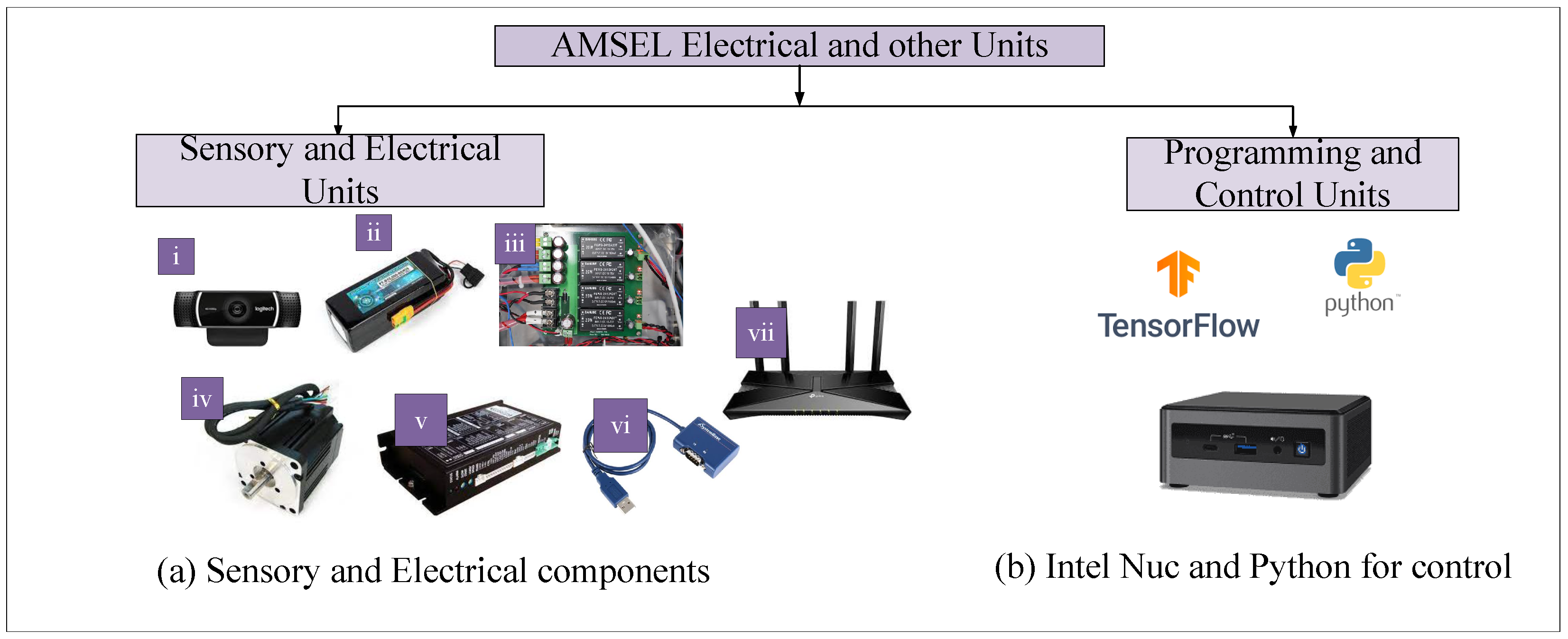
3.2.1. Electrical Units

The AMSEL robot’s electrical block consists of various devices, including a camera, battery, power supply board, DC motors, etc. A list and short description of the utilized electronic devices are provided below:

• Vision System: A Logitech c922 Pro HD Stream Webcam is been utilized as the vision system of the AMSEL robotic platform (Figure 3a (i)).
• Power source: In the AMSEL robot, a Polytronics Lithium-Polymer (Li-Po) battery is used as the power source. The model number of the utilized battery is PT-B16-Fx30 (Figure 3a (ii)).
• Power supply board: A custom-designed power supply board is utilized to split the power from the Li-Po battery among the other electronic devices used in the robotic platform (Figure 3a (iii)).
• DC motors: For navigating the robot, four DC motors are used in the AMSEL robot (Figure 3a (iv)). The DC motors used in this robot are 200W Brushless DC (BLDC) motors. The model number of these motors is TM90-D0231.
• BLDC motor controller: For driving and controlling the motors in the AMSEL robot, four BLDC motor controllers are used (Figure 3a (v)). The model number of the utilized controller is TMC-MD02.
• Serial communication adapter: The AMSEL robotic platform uses multiple serial communication adapters for converting the RS485 communication to USB communication, as the system’s main controller uses USB communication protocol (Figure 3a (vi)).
• Router: A Tplink Archer Ax73 outer is used in the AMSEL robot for communicating with the host PC in the ground station (Figure 3a (vii)).

3.2.2. Control Unit

The control system of the AMSEL robotic platform is divided into two parts: one is the software control unit, and the other one is the hardware control unit. For the software control, a graphical user interface (GUI) (Figure 4) is designed using the Python programming language and implemented on a host computer in the ground station.

The GUI communicates with the primary hardware controller of the AMSEL robot using socket communication technology, where the robotic platform works as the server and the host PC works as the client. The GUI has various buttons that are used to send commands to the robotic platform. The vehicle executes the corresponding commands and sends the image data to the host PC through the socket communication channel. The primary controller in the hardware is an Intel Nuc mini PC, with six cores and 8GB RAM, and it runs on Windows 10. The control unit in the hardware architecture comprises two control blocks, and all of them are controlled by the primary controller. Figure 5 displays the control blocks and the hardware architecture of the AMSEL platform.

From Figure 5, it can be seen that the hardware architecture of the AMSEL robot is composed of three control blocks, including a vision system unit associated with Deep Learning and a navigation control unit. The vision block comprises a Logitech C922 Pro HD webstream camera. The camera is powered by the intel nuc mini PC and communicates with it by using a USB 3.0 communication interface. For processing the images, deep learning frameworks (Tensorflow, Keras) were installed in the primary controller. This control block captures the images, detects cracks using deep learning technology, and passes the images to the host computer using server-client communication technology. The navigation control unit comprises the motor controllers and the motors, which are powered via the power supply board. The primary controller communicates with the motor controllers using serial communication technology. The primary controller sends the commands to the motor controller, and they drive the motors as per the commands. The motor controllers can also send the spatial encoder data to the primary controller for making decisions on navigation and generating the next commands.

4. Crack Detection and Quantification from Image

4.1. Proposed Architecture for Crack Segmentation

Crack detection can be considered a semantic segmentation [35,36] problem where the ‘crack’ and ‘non-crack’ pixels are assigned as two different classes. This paper proposes a novel lightweight (number of parameters: 981,723) crack-detection method named ‘RCDNet: Real-Time Crack Detection Network’ based on deep learning. This work has utilized the encoder-decoder architecture [37,38] as the base framework of our proposed model. The model was designed in such a way that it can exploit all the necessary information for good prediction with few model parameters and less computational complexity. The main purpose of reducing the model size is to make it compatible with implementing it on the onboard computer of the robotic platform and detecting cracks in real-time. The overall architecture of the proposed model is shown in Figure 6. As illustrated in Figure 6, our proposed model has two major parts, including a dual channel encoder module and a decoder module, while the encoder and the decoder parts contain attention modules [39], namely the context-embedded channel attention (CECA) module and the global attention module (GAM), respectively. The encoder part of our model extracts different levels of feature information (low-level to high-level) from the RGB images of size 512 × 512 in each of the encoder stages. This work utilizes a dual-channel encoder module for extracting information of different scales. Later, this paper fuses this multi-scale information at the beginning of the CECA module, which ensures the availability of more detailed and rich contextual information from the original images. After this multi-scale feature fusion, the CECA module passes the aggregated features through a channel attention branch to provide more weights to the most important channels of the feature map and thus produces a new channel-refined feature map. Then, the GAM in the decoder part collects the low-level features from the CECA modules and the upsampled high-level features from the convolution blocks of the decoder. GAM utilizes the high-level feature maps as the guide to weigh the low-level features and later fuses them with the high-level features. After that, the GAM module passes this weighted channel’s refined feature to a spatial attention branch to produce spatially refined features. The spatially refined features give more weight to important pixels of a channel for accurately predicting the cracks. Finally, after repeating the process in each stage of the decode block, our model gradually restores the feature maps and produces the segmentation map with the same resolution, as it is good to have the same resolution. The design of each branch of our model is discussed briefly in the following subsections.

4.1.1. Encoder Module

This work has designed a symmetric dual-channel encoder module for extracting information on different scales from pavement images. The purpose of using a dual-channel encoder module is to collect maximum information from the images by performing multi-scale feature fusion. The literature shows that in CNN convolution, the kernel size can be divided into two groups: small kernel size (1 × 1, 2 × 2, 3 × 3) and large kernel size (5 × 5, 7 × 7, 11 × 11). These two groups have different types of characteristics in the case of extracting features. The small kernels are more likely to extract local, complex, and fine-grained features. On the other hand, the large kernels have a larger receptive field and can extract widespread and global features. Conventional CNN models usually use either small kernels or large kernels in their network. However, many important pieces of information are overlooked and missed with this strategy, which hampers the accurate detection of cracks. To overcome this problem, in our network, this paper proposes a dual-channel encoder scheme so that the feature maps from each encoder stage can contain both rich spatial information and the precise location information of the cracks in pavement images. The kernel size utilized in the encoder channels of our network is 3 × 3 and 7 × 7. Both of the encoder channels of our proposed network consist of five encoder blocks, where each of the blocks is followed by a 2 × 2 maxpooling layer. The encoder blocks in our model consist of a convolution layer with the same number of filters for encoder channel 1 and encoder channel 2. The first two blocks used 16 filters, and the later ones utilized 32, 64, and 128 filters, respectively, to perform the convolution operation and extract feature maps of different numbers from every stage. The first encoder block of our network receives the original RGB images with the size of H × W × C, where H is the height, W is the weight of the images, and C represents the number of channels. After going through each of the encoder blocks, the images were downsampled by half due to the maxpooling layers, and the blocks produced feature maps as the number of utilized filters. So after the first encoder block in both of the channels, the output feature size becomes H/2 × W/2 × 16. And finally, at the end of the encoder module, this research obtains a feature map of size H/32 × W/32 × 128.

4.1.2. Context Embedded Channel Attention Module

After extracting features from the encoder channels, this research designs a context-embedded channel attention (CECA) module for fusing the information of the corresponding stages of every channel and recalibrating the extracted features based on the inter-channel relationships and dependencies. The main purpose of the CECA module is to give more weight to the important channels of a feature map and overlook the unnecessary ones to improve the feature representation. The structure of the proposed CECA module is shown in Figure 7.

As shown in Figure 7, our CECA module first takes the feature maps of the encoder channels f${}_{3\times 3}$, f${}_{7\times 7}$∈${\mathrm{ℝ}}^{H\times W\times C}$ as inputs and aggregates them to generate a context-embedded feature map F∈${\mathrm{ℝ}}^{H\times W\times C}$. In the later part of the CECA module, the embedded feature map F is passed through two parallel branches of the global average pooling (G${}_{ap}$) layer and the global maxpooling (G${}_{mp}$) layer. The G${}_{ap}$ layer produces a descriptor feature d${}_a$∈${\mathrm{ℝ}}^{C\times 1\times 1}$ that contains the information of channel statistics by consolidating the spatial information. And the feature d${}_m$∈${\mathrm{ℝ}}^{C\times 1\times 1}$ produced from the G${}_{mp}$ layer contains important information about the object features. Mathematically,

$$\begin{array}{c}\hfill d_a=G_{ap}\left(F\right)\\ \hfill d_m=G_{mp}\left(F\right)\end{array}$$

(1)

The descriptor features d${}_a$ and d${}_m$ are then fed to a shared MLP layer for attaining the degree of association among the channels. For reducing the computational complexities, the number of hidden layers was selected as ${\mathrm{ℝ}}^{C/r\times 1\times 1}$, where r is the reduction ratio. At the end of the parallelly branched MLP layers, the outputs are fused and passed through a sigmoid activation function to generate a feature map V.

$$V=\sigma \{\mathrm{MLP}\left[d_a\right]+\mathrm{MLP}\left[d_m\right]\}$$

(2)

Finally, the output of our CECA module B ∈${\mathrm{ℝ}}^{H\times W\times C}$ is obtained by multiplying the original feature maps from the encoder stages with the feature map V. So the CECA is defined as follows:

$$B=V\otimes f_{3\times 3}\otimes f_{7\times 7}$$

(3)

Therefore, using the CECA blocks, this work obtains refined activation maps that focus more on important channels and suppress the unnecessary ones. The size of the refined activation maps is the same as the intermediate activation maps extracted from the encoder stages.

4.1.3. Decoder with Global Attention Module

The decoder module of our proposed model consists of five convolution blocks and four global attention module (GAM) blocks. Each of the convolution blocks consists of two convolution layers, which have the same number of filters corresponding to the encoder blocks. The convolutional layers are followed by a Rectified Linear Unit (ReLU) activation function and a batch normalization layer. The size of the kernels utilized in the decoder layers is 3 × 3. In the GAM blocks, this work fuses the upsampled high-level feature X${}_h$∈${\mathrm{ℝ}}^{H\times W\times 2C}$ generated by the convolution blocks in the previous decoder stage and the low-level features X${}_l$∈${\mathrm{ℝ}}^{H\times W\times C}$ generated by the CECA module. However, as shown in Figure 8, before fusing the features from different stages, the GAM module weighs the low-level features based on the high-level features to put more focus on the key information. To generate the weighted features, GAM first performs a 3 × 3 convolution on the low-level features. And the high-level features are passed through the channel attention block of the CECA module to assign more weights to the important channels and recalibrate the high-level features. Then, the low-level features and high-level features are multiplied to generate weighted low-level features ∈${\mathrm{ℝ}}^{H\times W\times C}$. Later, the original high-level feature map x${}_h$ is compressed by passing through a 1 × 1 convolution layer to achieve the same dimension as x${}_l$. At the end of this stage, the weighted low-level features and high-level features are merged to produce a channel-refined feature y${}_0$∈${\mathrm{ℝ}}^{H\times W\times C}$. Mathematically,

$$\begin{array}{c}\hfill y_0=E+con{v}^{1\times 1}\left(x_h\right)\\ \hfill y_0=con{v}^{3\times 3}\left(x_l\right)+V\left(x_h\right)+con{v}^{1\times 1}\left(x_h\right)\end{array}$$

(4)

After obtaining the channel-refined feature, GAM performs spatial attention on the y${}_0$ to extract the spatial interpixel relations. The primary goal of utilizing spatial attention is to focus on the important pixels of a channel that highlight meaningful features to provide prospective crack information. To perform the spatial attention, the channel refined feature y${}_0$ is passed through an average pooling and maxpooling layer along with the spatial dimension. As a result, this process generates two feature maps:

$$\begin{array}{c}\hfill q_{ap}=a_p\left(y_0\right)\\ \hfill q_{mp}=m_p\left(y_0\right)\end{array}$$

(5)

Then these two-dimensional outputs, q${}_{ap}$∈${\mathrm{ℝ}}^{1\times H\times W}$ and q${}_{mp}$∈${\mathrm{ℝ}}^{1\times H\times W}$, are concatenated as

$$Q=(q_{ap},q_{mp})$$

(6)

After this step, the concatenated feature map goes through a 7 × 7 convolution layer followed by a sigmoid activation function. This work finally obtains the feature map S ∈${\mathrm{ℝ}}^{H\times W\times C}$. The output activation map S from the GAM block contains the most essential pixel information for detecting cracks as it is filtered out in both the spatial and channel-wise dimensions. This output is then fed into a convolutional layer of the next decoder stage for reconstructing the pixels and predicting the cracks on road images. Following this process in all the five decoder blocks, this process generates a feature map of size H × W × 16. Later, this process applies a 1 × 1 convolution to obtain the predicted image with the same shape (H × W × C) as the original image.

4.2. Dataset Description and Training of the Model

4.2.1. Dataset

The dataset utilized in this process for training the crack segmentation model is a public benchmark dataset named the Crack500 dataset [40]. The dataset was collected using smart mobile phones from the main campus of Temple University, USA. The researchers initially collected 500 images with a resolution of 2000 × 1500 pixels. Considering the issue of a small number of images and the large size of the images, each image was cropped into 16 non-overlapping parts. The researchers only kept the regions with resolutions of more than 1000 pixels. Consequently, the final dataset contains 3368 images. The dataset also provides annotated ground truth for each of the images.

4.2.2. Implementation Details

The crack-segmentation problem can be considered a class imbalance problem since the number of pixels containing cracks can be very low. Therefore, to handle the class imbalance problem during crack estimation, this work has used the dice loss function in this work. The dice loss function can be calculated using the following formula:

$$DiceLoss=1-{\displaystyle \frac{2{\sum }_i{m}_i{n}_i+\gamma }{m_i^2+n_i^2+\gamma }}$$

(7)

where m represents the predicted probabilities of the classes, n denotes the ground truth data, and $\gamma$ denotes the smoothing factor. This work divided the dataset into 7:3 for training and testing the model and resized input images and ground truths in the size of (512 × 512 × 3) and (512 × 512 × 3), respectively. This work chose the Adam optimizer to optimize our model. This work set the batch size to 2 and the learning rate to 0.001 and trained the model to the 100th epoch. This work utilized Python version 3.6.13 as the development language and Keras version 2.6.0 as the Deep Learning framework. We trained the model and conducted our experiments in a computer configured with a Windows 10 operating system, 32 GB RAM, Intel core i9-11900k @ 3.50 GHz CPU processor, and NVIDIA Geforce RTX 3080Ti graphics card.

4.3. Crack Severity Analysis

The proposed model provides us with the segmented cracks from the images. However, we also needed to determine the number of cracks and other morphological features (e.g., length, maximum width, area, density) to analyze the severity of cracks in any particular sample picture. To do so, this work utilized the conventional image-processing technique described below.

4.3.1. Counting the Cracks

In the first step of our crack-severity-analysis section, this work calculated the number of individual cracks in railway sleeper images. To count the cracks, this work utilized the concept of contour detection in the images. Contour detection is a process that can be explained as a closed curve with an orientation that joins all the continuous points (along with the boundaries) with similar pixel intensities. Consider an image as a 2D function f(x,y); then,

$$f(x,y)=c$$

(8)

where c is the constant pixel value. So, using the contour detection process, this work obtains the connected regions of the crack denoting pixels predicted by the proposed model and crack boundaries. Thus, this work can calculate the number of detected contours, i.e., the number of individual crack objects.

4.3.2. Extracting Morphological Features

After extracting the individual crack objects from the previous step, this work calculated the cracks’ morphological features (length, width, area, and density). To calculate the length and the maximum width of the cracks, this work applied Algorithm 1. From the previous section, this work generated the boundaries of the contours, i.e., cracks. Consider a contour C = [X,Y], which is an array of two columns with N length, where, $x_0$, $x_1$,……$x_n$∈ X denotes the rows of the image and $y_0$, $y_1$,……$y_n$∈ Y denotes the columns of the image. Let ($x_0$, $y_0$) and ($x_n$, $y_n$) be the starting point and the ending point of the contour, i.e., crack, respectively. To find out the length of the crack, this work calculated the distance between the starting point and the ending point of the crack boundary using the distance formula. To calculate the maximum width of a crack, this work first decided whether the crack is horizontal or longitudinal in nature based on the number of rows and columns of the image inside the contour. If the crack has more columns than rows, then the crack is horizontal as its length is toward the horizontal direction of the image frame. On the other hand, a crack is longitudinal if the contour has more rows. To find the maximum width of a horizontal crack, this work traversed from the starting column $y_0$ to the ending column $y_n$ of the crack boundary. During this process, this work located and stored the rows where any particular column $y_j$ was examined in a list named occurs. This work estimated the number of rows traveled by any column $y_j$ when this searching loop was completed, and this work appended the results for each column to a list entitled widths. Finally, this work searched for the maximum value in the list, and this work thus calculated the maximum width of a crack. Furthermore, this work also estimated the location of the maximum width of the crack. To do so, this work found the position of the first and last rows of the column, which had been examined as maximum rows. To find the width of a longitudinal crack, this work utilized the same process; however, this time, this work examined the rows from $x_0$ to $x_n$ and stored the number of columns traversed by a particular row $x_j$. Later, on the basis of these, this work estimated the maximum number of columns traversed by a particular row $x_j$, which represents the maximum width of a longitudinal crack. This work calculated the area of the contours as the area of the individual cracks. After that, this work added the area of the individual cracks and calculated the total area covered by the cracks in the image. Finally, this work divided the total area of the cracks by the number of pixels to obtain the density of the cracks in an image.

Algorithm 1: Algorithm for length and width calculation

5. AMSEL Robot Working Method

The AMSEL robot platform conducts data collection and data processing fully autonomously. The working principle of the AMSEL platform is illustrated in Figure 9.

As can be seen from Figure 9, the robotic system is divided into two working stations, i.e., the robot device and the host computer. The AMSEL robot navigates on the concrete pavement and collects images from the surface. The robot collects images from a height of 30 cm, and the area covered by one image is 302 mm × 227 mm. After collecting the image data with a resolution of 640 × 480 pixels, the onboard computer of the AMSEL platform resizes the image to a resolution of 512 × 512 pixels and segments the cracks in the collected picture by utilizing the proposed deep-learning model described in Section 4.1. Then, the robot transmits the processed image to the host computer in real time. Finally, the host computer shows the image in the user interface of the robotic system and stores it on the device to further analyze the crack severity using the algorithm described in Section 4.3.

5.1. Manual Navigation and Pavement Inspection

In manual mode, the robot’s movement and pavement are inspected by a user with the user interface of the AMSEL robot system. The user interface has four navigation buttons, i.e., Forward, Backward, Right, and Left. The user navigates the robot using these buttons to the place where they want to go. To navigate manually, the user can control the speed of the robot as well by sending a specified velocity in RPM to the robot. The user has the flexibility to place the robot in any position and orientation in this manual mode. Figure 10 shows the manual inspection process in both indoor and outdoor environments. During the navigation, the user turns on the camera by pressing the “Video” button on the UI and checks whether there is a crack or not in a certain location by monitoring the video display portion of the UI.

5.2. Automated Navigation and Pavement Inspection

In the automated navigation process, the AMSEL robot navigates through a predefined survey area. The navigation area is a rectangle with a width of a meters and a length of b meters, where the robot takes a,b as input from the user interface at the host computer. When the robot receives inputs and commands to move autonomously, it starts navigating automatically and collecting data lane by lane. The number of lanes depends on the width of the survey area. Figure 11 is a diagram of the survey area. The AMSEL robot follows stop and go, a certain distance method for conducting the pavement inspection process. In this work, the AMSEL robot goes for 25 cm and stops to collect NDE data. The distance of 25 cm between two consecutive lanes is also selected in this work. Algorithm 2 displays the method of the AMSEL robot’s automated navigation and pavement procedure. Figure 12 shows the automated inspection process in the outdoor environment. From Algorithm 2, it can be seen that, after obtaining the command of the automated navigation, the AMSEL robot calculates the number of lanes n${}_l$ and the number of steps n${}_s$ in each lane. The number of lanes n${}_l$ is determined by dividing the width a of the survey area by 0.25, as the distance between two lanes is 25 cm. And the number of steps n${}_s$ is determined by dividing the length of the survey area by 0.25, as the robot will move 25 cm in each step. Then, the robot starts performing the assigned tasks in the steps. First, the robot captures one picture and detects cracks in it. After cracks are detected in the picture, the picture is transferred to the host computer along with the robot location on the survey grid and the density of cracks in the image. Then, the robot moves directly to the next scanning location. To navigate the correct distance and place the robot in the precise position, this work calibrated the spatial encoder data of the motors. After calibration, this work found that to move 1 m, wheels must change their position by 1176 points.

Algorithm 2: Algorithm for automated navigation and inspection

On this basis, this work calculated the value to navigate 25 cm. By considering the change in position of the wheels, this work also calibrated for the left and right turns by 90${}^{\circ }$. When the robot completes all the steps on a lane, it checks whether it is an odd or even lane. If it is an odd lane, the robot turns right, moves 25 cm, and turns right again to place itself at the beginning of the next lane. On the other hand, if the lane is an even lane, the robot turns left, moves 25 cm, and turns left again to place it at the beginning of the next lane. The robot continues these processes till it completes the scanning of the last lane. After the last lane is complete, it again checks whether the last is odd or even. If the last lane is odd, the robot turns left and navigates the a meter distance, turns left again, and navigates the b meter distance. After this, it makes a 360${}^{\circ }$ turn to go back to the starting position and orientation of the robot. On the contrary, if the final lane is even, the robot turns right, navigates the a meter distance, and turns right again to go back to the starting position and orientation of the robot.

6. Results and Discussion

6.1. Performance of the Deep Learning Model

This work has used one segmentation model named RCDNet to predict the images. To evaluate the performance of our proposed RCDNet, this work used four metrics: accuracy, intersection over union, Dice loss, and Dice coefficient. The percentage of successfully categorized pixels is referred to as pixel accuracy while a binary segmentation task is being performed. However, due to the class imbalance issue, pixel accuracy is not the best metric to evaluate the segmentation task. For the majority of the non-lane pixels in the case of lane detection, the images in the dataset are severely unbalanced. The Dice coefficient and the IOU, on the other hand, are seen to be more useful metrics because they depend on the overlap between the anticipated picture and the ground truth image. The metrics can be mathematically represented using the following equation.

$$\begin{array}{c}\hfill \mathrm{Dice}\mathrm{Coefficient}=\frac{2\sum {\mathrm{Y}}_{\mathrm{p}}{\mathrm{Y}}_{\mathrm{t}}}{\sum {\mathrm{Y}}_{\mathrm{p}}+\sum {\mathrm{Y}}_{\mathrm{t}}}\\ \hfill \mathrm{IoU}=\frac{\sum {\mathrm{Y}}_{\mathrm{p}}{\mathrm{Y}}_{\mathrm{t}}}{(\sum {\mathrm{Y}}_{\mathrm{p}}+\sum {\mathrm{Y}}_{\mathrm{t}})-(\sum {\mathrm{Y}}_{\mathrm{p}}{\mathrm{Y}}_{\mathrm{g}})}\end{array}$$

(9)

The calculation demonstrates that the Dice coefficient represents the sum of the pixels in the two overlapping regions. The IOU also stands for the region of overlap between the expected and actual images, which is delineated by the union area. Figure 13 displays the accuracy, loss, Dice coefficient, and IoU trend for our proposed model over both the training and test sets.

From Figure 13, it can be seen that our model was trained well. There is not much difference between the curves of the training set and the test set, which indicates that the model did not experience underfitting or overfitting. The training curves for all the metrics did not fluctuate throughout all the epochs. Between the first and about the third epochs of our model, the test curves began to rise quickly. But starting with the third epoch, it gradually increased and began to stabilize. Around the 27th, 52nd, 84th, and 97th, they went through four minor oscillations of varying degrees. However, our model was able to handle this variation, and starting with the very next epochs, the curves stabilized once more. Finally, our model showed promising results in terms of metrics.

Table 3. RCDNet model performance in both the training and testing set.

	Accuracy (%)	Dice Coefficient (%)	IoU (%)	Dice Loss (%)
Train set	96.35	97.40	97.35	0.0180
Test set	96.29	97.33	96.90	0.0214

presents the result of our developed model from the perspective of the previously mentioned metrics on both the training set and the test set.

6.2. Comparison with Other State-of-the-Art Methods

In this section, we discuss the performance comparison of the proposed RCDNet with other popular semantic segmentation frameworks, namely FCN-8, SegNet, and U-Net. These models were trained using the same dataset and on the same GPU card. The performance comparison was based on standard evaluation metrics. According to

Table 4. Segmentation comparison of our RCDNet and other representative methods.

Network	Accuracy (%)	Dice Coefficient (%)	IoU (%)	Number of Parameters (M)
FCN	93.20	93.16	92.93	134.27
SegNet	95.60	95.83	94.44	29.44
U-Net	96.33	98.40	97.92	13.40
RCDNet	96.29	97.33	96.90	0.91

, the proposed RCDNet outperforms FCN and SegNet methods by 2–4% in terms of Dice and IoU scores. The parameter count of the proposed RCDNet is also less than that of the FCN and SegNet. It is worth noting that U-Net achieves better performance than our model; however, our model has fewer parameters compared to U-Net. This indicates that despite a marginal difference in performance metrics, our model is a better choice for implementing a real-time crack detection system due to its lower parameter count.

6.3. Pavement Assessment in Manual Mode

For the manual assessment of the pavement, the AMSEL robotic platform was navigated by an operator in both indoor and outdoor environments. The robot moved to different places and collected pictures using its visual sensor. The onboard computer segmented the crack pixels and sent the predicted images to the ground stations. After generating the segmented results from the RCDNet, this work measured the length, width, area, and density of the cracks. Though the crack measurement algorithm produces the result in a pixel unit, the size of the cracks in the physical unit can be calculated easily. As the vision sensor of the robotic system can cover an area of 302 mm × 227 mm with a pixel resolution of 640 × 480, one pixel is about 0.47 mm both in height and width of the picture. Furthermore, this work compared these results with manually measured data. In this study, the severity of the cracks was also assessed. The density of the cracks was calculated as the ratio of the cracked pixels and the total pixels of an image. The severity scale density used in this work is shown in

Table 5. Assessing the severity of road cracks.

Measurements (M)	Severity	Limit
Area (mm)	Fair	M < 0.4%
	Poor	0.4% ≤ M < 1%
	Severe	M > 1%

. Figure 14 and Figure 15 show the original images, estimated black and white images, overlapped images, and the images after the crack-measurement algorithm was performed in indoor and outdoor environments, respectively.

Table 6. Comparison between the manually measured and digitally measured crack size in the indoor environment.

Picture	Number of Cracks	Manual Length	Manual Maximum Width	No of Cracks after Prediction	Digital Length	Digital Maximum Width	Area	Density	Severity
1.jpg	1	227 mm	10 mm	1	227.45 mm	8.93 mm	1039.75 mm${}^2$	1.44%.	Severe
2.jpg	2	72 mm, 187 mm	3 mm, 7 mm	2	72.04 mm, 178.75 mm	2.82 mm, 7.52 mm	484.675 mm${}^2$	0.67%.	Poor
3.jpg	1	302 mm	17 mm	1	295.91 mm	15.97 mm	2123.575 mm${}^2$	2.94%.	Severe
4.jpg	1	150 mm	5 mm	1	157.67 mm	5.11 mm	318.66 mm${}^2$	0.44%.	Poor
5.jpg	Web crack	-	-	Web crack	-	-	4330.93 mm${}^2$	6%.	Severe
6.jpg	1	240 mm	5 mm	1	232.56 mm	5.64 mm	344.98 mm${}^2$	0.47%.	Poor
7.jpg	1	325 mm	8 mm	1	312.24 mm	7.82 mm	545.32 mm${}^2$	0.83%.	Poor
8.jpg	Web crack	-	-	Web crack	- mm	-	599.83 mm${}^2$	0.88%.	Poor
9.jpg	1	302 mm	9 mm	1	302 mm	8 mm	1227.775 mm${}^2$	1.70%.	Severe
10.jpg	1	200 mm	3 mm	1	192.28 mm	2.82 mm	200.33 mm${}^2$	0.32%.	Fair

and

Table 7. Comparison between the manually measured and digitally measured crack size in the outdoor environment.

Picture	Number of Cracks	Manual Length	Manual Maximum Width	No of Cracks after Prediction	Digital Length	Digital Maximum Width	Area	Density	Severity
11.jpg	1	232 mm	8 mm	1	224.87 mm	7.52 mm	1144.09 mm${}^2$	1.59%.	Severe
12.jpg	1	307 mm	10 mm	1	300.86 mm	10.81 mm	1912.665 mm${}^2$	2.65%.	Severe
13.jpg	Web crack	-	-	Web crack	-	-	2747.5 mm${}^2$	3.81%.	Severe
14.jpg	Web crack	-	-	Web crack	-	-	3699.37 mm${}^2$	5.12%.	Severe
15.jpg	1	351 mm	17 mm	1	341.33 mm	15.81 mm	1713.26 mm${}^2$	2.37%.	Severe
16.jpg	1	240 mm	9 mm	1	225.67 mm	18.33 mm	1712.32 mm${}^2$	2.37%.	Severe
17.jpg	2	312 mm, 255 mm	9 mm,6 mm	2	305.15 mm, 238.87 mm	8 mm, 6.11 mm	2575.13 mm${}^2$	3.56%.	Severe
18.jpg	1	323 mm	10 mm	1	306.92 mm	10.81 mm	1841.572 mm${}^2$	2.55%.	Severe
19.jpg	2	268 mm, 98 mm	8 mm,18 mm	2	253 mm, 63.92 mm	8.46 mm, 17.86 mm	1487.54 mm${}^2$	2.06%.	Severe
20.jpg	1	230 mm	9 mm	1	224.43 mm	10 mm	1179.81 mm${}^2$	1.63%.	Severe

show the comparison between the manually collected data and the digitally extracted data and show the severity in indoor and outdoor environments, respectively.

From Figure 14, it can be seen that all the cracks are estimated well in the indoor environment. Even in the presence of shadows (Image2, Image3, Image5) and external noise (Image9), the RCDNet model detected the cracks accurately. However, if we observe Image2, Image8, and Image10 very closely, it can be noticed that there is some discontinuity in the detection. A very small portion of the cracks is not detected in the images. This work manually measured the widths of those portions and found the limitation of our proposed RCDNet, which is that it cannot detect cracks with widths less than 1mm from a 30 cm height. From Table 6, it can be seen that the difference between the manually measured data (length, width) and the digitally measured data of the cracks is very small for indoor images. This work has found that the average error rate of the measurements is 2.219% and 6.155%, respectively, for the length and maximum width. One finding is that the table shows more errors in the case of width calculation. However, this study believes that this large error was due to the ambiguity of determining cracks with the scale using the naked eye.

For the outdoor environment, in Figure 15, it can be seen that all the images are estimated accurately. However, if we take a closer look at Image12, Image13, Image14, and Image19, there is some error. From Image12, the finding is that, when the sunshine is extreme and there is a dark shadow, our model may interpret the shadow line as a crack. In Image13 and Image19, small portions of the cracks are not detected. The problem is that the depth between the edges of the cracks is very small, which looks not like a crack but rather a scratch on the pavement. However, the overall prediction in the outdoor environment is also quite accurate. From Table 7, it can be seen that the difference between the manually measured data and the digitally measured data is also very small in the outdoor images, similar to the indoor images. The relative error rates of these measurements are 6.703% and 5.631%, respectively. The unexpected finding from this table is the error rate in the length calculation. However, we can observe that Image19, which has two cracks, is not predicted accurately due to the lower depth and shows a large deviation in error. And this deviation affects the average error rate.

We also performed a linear regression between the manually measured and digitally measured length and width of the cracks to check the stability of the digitally measured data for both indoor and outdoor data. The linear regression for both indoor data and outdoor data in Figure 16a–d shows that the value of R${}^2$ in both cases (i.e., length and width) is close to 1. In addition, the noteworthy finding is that the regression efficiency for both data is also close to 1. This clearly indicates that the proposed system has good absolute accuracy for the length and width measurement of cracks.

In the case of the severity of indoor images, this work found that among the ten images, four images are in severe condition. Among the severe cracks, Image 5 is the most severe (6% cracked). Of the other images, five images are in poor crack condition and one image is in fair crack condition. Among the outdoor images, this work found that all the cracks are in severe condition. Among them, Image4 has the highest rank (5.12% severe).

6.4. Pavement Assessment in Automated Mode

The autonomous pavement assessment of the AMSEL robot was tested in both indoor and outdoor environments. For the automated assessment of the AMSEL robot in the indoor environment, this work chose a 3 m × 2 m grid in the parking lot of Dong-A University, Busan, South Korea. The AMSEL robot took around 10 min to inspect the 3 m × 2 m grid. For the outdoor environment, this work chose a 2.5 m × 1 m grid in the outdoor parking lot of Dong-A University, Busan, South Korea. The AMSEL robot took around 6 min to inspect the 2.5 m × 1 m grid, which is faster than manual inspection. In the indoor and outdoor environments, the robot collected and predicted 108 and 50 images, respectively. Figure 17 and Figure 18 show the stitched picture after segmenting the cracks of each location in indoor and outdoor environments, respectively.

The AMSEL robot platform also calculates the area of the cracks in each image and the density of the cracks to show the severity at each location. The area and severity of each location in the indoor and outdoor environments are illustrated in Figure 19a–d, where the horizontal and the vertical coordinates of the figure represent the distance of the grid blocks (a 3 m × 2 m grid for the indoor environment and a 2.5 m × 1 m grid for the outdoor environment) from the initial position in units of meters.

By analyzing Figure 19a–d, this work has found the severity statistics and the most severe locations in both the indoor and outdoor grids.

Table 8. Statistics of the detected cracks for indoor area shown in Figure 17.

Number of Cracks	Maximum Area	Minimum Area	Total Area	Total Density
43	3841.995 mm${}^2$, Loc. (x = 0 m, y = 0.25 m)	38.305 mm${}^2$, Loc. (x = 2 m, y = 3 m)	22,617.69 mm${}^2$	0.38%

and

Table 9. Statistics of the detected cracks for the outdoor area shown in Figure 18.

Number of Cracks	Maximum Area	Minimum Area	Total Area	Total Density
18	1741.35 mm${}^2$, Loc. (x = 0.5 m, y = 0.25 m)	308.2025 mm${}^2$, Loc. (x = 0.75 m, y = 0.5 m)	15,231.88 mm${}^2$	0.68%

show the statistics of the detected cracks in the indoor and outdoor grid, respectively.

From Table 8, it can be seen that among the 108 images, a total of 43 images contain cracks in the indoor grid. Among the cracks, for the crack in the location of the first lane, the first stoppage has a maximum area of 3,841.995 mm${}^2$, and for the crack in the location of the last lane, the last stoppage has a minimum area of 38.305 mm${}^2$. The total cracked area is 22,617.69 mm${}^2$, and 0.38% of the grid’s total area is cracked. From Table 9, it can be seen that among the 50 images total of 18 images contain cracks on the grid. Among the cracks, for the crack in the location of the third lane, the first stoppage has a maximum area of 1741.35 mm${}^2$, and for the crack in the location of the fourth lane, the second stoppage has a minimum area of 308.2025${}^2$. The total cracked area is 15,231.88 mm${}^2$, and 0.60% of the grid’s total area is cracked.

7. Drawbacks of the Proposed System

Though the proposed system demonstrated promising results for estimating cracks in concrete pavements in both indoor and outdoor environments, the current version of the proposed system has a few drawbacks. The primary drawbacks are as follows.

• The proposed DL model named RCDNet cannot detect cracks with widths less than 1 mm from a 30 cm height.
• When the sunshine is extreme and there is a dark shadow in the outdoor environment, the RCDNet may predict a shadow line as a crack.
• The RCDNet fails if the depth between the edges of the crack is very small, such that it does not look like a crack but rather a scratch on the pavement.
• The robotic vehicle occasionally encounters a slight deviation from the linear path during automated navigation, which poses challenges in reestablishing its initial pose upon returning to the starting position.
• The camera’s frame size was slightly larger than the gap between the two consecutive lanes, causing a small overlap in the captured images.

Despite some inherent drawbacks, the proposed robotic system exhibits promising results and serves as a compelling solution for effectively monitoring pavement cracks, thereby reducing human labor, costs, and inspection time.

8. Conclusions

In this work, a semi-automated robotic platform named AMSEL has inspected pavement cracks in real-time. An encoder–decoder-based lightweight deep learning model named RCDNet was proposed to detect pavement cracks. The robotic platform was developed for manual and automated navigation to complete the inspection. Both indoors and outdoors, the robot was able to navigate and accurately collect and analyze the data. Extensive testing and deployment of the AMSEL showed the advantage over manual testing during pavement-crack inspection and evaluation. A crack severity map was also generated based on the analysis of image data from the robot to provide a simple and efficient way to monitor pavement cracks. In future work, this work plans to integrate NDE sensors, including IE, GPR, USW, ER, etc. Future research will add multiple visual sensors to cover a large area quickly to make the inspection process faster. Finally, our plan is to fuse all sensor data and develop a deep-learning model to obtain various defect information and construct a correlation model among the NDE sensors.

References

1. Lee, R.B. Development of korean highway capacity manual. In Highway Capacity and Level of Service; Routledge: London, UK, 2021; pp. 233–238. [Google Scholar]
2. Chen, C.; Seo, H.; Jun, C.; Zhao, Y. A potential crack region method to detect crack using image processing of multiple thresholding. Signal Image Video Process. 2022, 16, 1673–1681. [Google Scholar] [CrossRef]
3. Akagic, A.; Buza, E.; Omanovic, S.; Karabegovic, A. Pavement crack detection using otsu thresholding for image segmentation. In Proceedings of the 2018 41st International Convention on Information and Communication Technology, Electronics and Microelectronics (MIPRO), Opatija, Croatia, 21–25 May 2018. [Google Scholar]
4. Nigam, R.; Singh, S.K. Crack detection in a beam using wavelet transform and photographic measurements. Structures 2020, 25, 436–447. [Google Scholar] [CrossRef]
5. Zoubir, H.; Rguig, M.; Aroussi, M.E.; Chehri, A.; Saadane, R. Concrete Bridge Crack Image Classification Using Histograms of Oriented Gradients, Uniform Local Binary Patterns, and Kernel Principal Component Analysis. Electronics 2022, 11, 3357. [Google Scholar] [CrossRef]
6. Gehri, N.; Mata-Falcón, J.; Kaufmann, W. Automated crack detection and measurement based on digital image correlation. Constr. Build. Mater. 2020, 256, 119383. [Google Scholar] [CrossRef]
7. Medina, R.; Llamas, J.; Gómez-García-Bermejo, J.; Zalama, E.; Segarra, M.J. Crack Detection in Concrete Tunnels Using a Gabor Filter Invariant to Rotation. Sensors 2017, 17, 1670. [Google Scholar] [CrossRef] [Green Version]
8. Nguyen, H.-N.; Kam, T.-Y.; Cheng, P.-Y. An Automatic Approach for Accurate Edge Detection of Concrete Crack Utilizing 2D Geometric Features of Crack. J. Signal Process. Syst. 2013, 77, 221–240. [Google Scholar] [CrossRef]
9. Chun, P.; Izumi, S.; Yamane, T. Automatic detection method of cracks from concrete surface imagery using two-step light gradient boosting machine. Comput.-Aided Civ. Infrastruct. Eng. 2020, 36, 61–72. [Google Scholar] [CrossRef]
10. Vedrtnam, A.; Kumar, S.; Barluenga, G.; Chaturvedi, S. Early crack detection using modified spectral clustering method assisted with FE analysis for distress anticipation in cement-based composites. Sci. Rep. 2021, 11, 1–19. [Google Scholar] [CrossRef]
11. Zhang, L.; Yang, F.; Zhang, Y.D.; Zhu, Y.J. Road crack detection using deep convolutional neural network. In Proceedings of the 2016 IEEE International Conference on Image Processing (ICIP), Phoenix, AZ, USA, 25–28 September 2016. [Google Scholar]
12. Cha, Y.-J.; Choi, W.; Büyüköztürk, O. Deep Learning-Based Crack Damage Detection Using Convolutional Neural Networks. Comput. Civ. Infrastruct. Eng. 2017, 32, 361–378. [Google Scholar] [CrossRef]
13. Eisenbach, M.; Stricker, R.; Seichter, D.; Amende, K.; Debes, K.; Sesselmann, M.; Ebersbach, D.; Stoeckert, U.; Gross, H.-M. How to get pavement distress detection ready for deep learning? A systematic approach. In Proceedings of the 2017 International Joint Conference on Neural Networks (IJCNN), Anchorage, AK, USA, 14–19 May 2017; pp. 2039–2047. [Google Scholar]
14. Li, Y.; Han, Z.; Xu, H.; Liu, L.; Li, X.; Zhang, K. YOLOv3-Lite: A Lightweight Crack Detection Network for Aircraft Structure Based on Depthwise Separable Convolutions. Appl. Sci. 2019, 9, 3781. [Google Scholar] [CrossRef] [Green Version]
15. Li, L.; Zheng, S.; Wang, C.; Zhao, S.; Chai, X.; Peng, L.; Tong, Q.; Wang, J. Crack Detection Method of Sleeper Based on Cascade Convolutional Neural Network. J. Adv. Transp. 2022, 2022, 1–14. [Google Scholar] [CrossRef]
16. Yang, X.; Li, H.; Yu, Y.; Luo, X.; Huang, T.; Yang, X. Automatic Pixel-Level Crack Detection and Measurement Using Fully Convolutional Network. Comput.-Aided Civil Infrastruct. Eng. 2018, 33, 1090–1109. [Google Scholar] [CrossRef]
17. Polovnikov, V.; Alekseev, D.; Vinogradov, I.; Lashkia, G.V. DAUNet: Deep Augmented Neural Network for Pavement Crack Segmentation. IEEE Access 2021, 9, 125714–125723. [Google Scholar] [CrossRef]
18. Yong, P.; Wang, N. RIIAnet: A Real-Time Segmentation Network Integrated with Multi-Type Features of Different Depths for Pavement Cracks. Appl. Sci. 2022, 12, 7066. [Google Scholar] [CrossRef]
19. Yu, S.N.; Jang, J.-H.; Han, C.-S. Auto inspection system using a mobile robot for detecting concrete cracks in a tunnel. Autom. Constr. 2007, 16, 255–261. [Google Scholar] [CrossRef]
20. Lei, B.; Ren, Y.; Wang, N.; Huo, L.; Song, G. Design of a new low-cost unmanned aerial vehicle and vision-based concrete crack inspection method. Struct. Heal. Monit. 2020, 19, 1871–1883. [Google Scholar] [CrossRef]
21. Oyekola, P.; Mohamed, A.; Pumwa, J. Robotic model for unmanned crack and corrosion inspection. Int. J. Innov. Technol. Explor. Eng. 2019, 9, 862–867. [Google Scholar] [CrossRef]
22. Li, H.; Song, D.; Liu, Y.; Li, B. Automatic Pavement Crack Detection by Multi-Scale Image Fusion. IEEE Trans. Intell. Transp. Syst. 2018, 20, 2025–2036. [Google Scholar] [CrossRef]
23. La, H.M.; Dinh, T.H.; Pham, N.H.; Ha, Q.P.; Pham, A.Q. Automated robotic monitoring and inspection of steel structures and bridges. Robotica 2018, 37, 947–967. [Google Scholar] [CrossRef] [Green Version]
24. La, H.M.; Gucunski, N.; Dana, K.; Kee, S.-H. Development of an autonomous bridge deck inspection robotic system. J. Field Robot. 2017, 34, 1489–1504. [Google Scholar] [CrossRef] [Green Version]
25. Kolvenbach, H.; Valsecchi, G.; Grandia, R.; Ruiz, A.; Jenelten, F.; Hutter, M. Tactile inspection of concrete deterioration in sewers with legged robots. In Proceedings of the 12th Conference on Field and Service Robotics (FSR 2019), Tokyo, Japan, 29–31 August 2019. [Google Scholar]
26. Le, D.V.K.; Chen, Z.; Rajkumar, R. Multi-sensors in-line inspection robot for pipe flaws detection. IET Sci. Meas. Technol. 2020, 14, 71–82. [Google Scholar] [CrossRef]
27. Pan, Y.; Zhang, X.; Cervone, G.; Yang, L. Detection of Asphalt Pavement Potholes and Cracks Based on the Unmanned Aerial Vehicle Multispectral Imagery. IEEE J. Sel. Top. Appl. Earth Obs. Remote Sens. 2018, 11, 3701–3712. [Google Scholar] [CrossRef]
28. Montero, R.; Menendez, E.; Victores, J.G.; Balaguer, C. Intelligent robotic system for autonomous crack detection and caracterization in concrete tunnels. In Proceedings of the 2017 IEEE International Conference on Autonomous Robot Systems and Competitions (ICARSC), Coimbra, Portugal, 26–28 April 2017. [Google Scholar]
29. Yang, L.; Li, B.; Li, W.; Brand, H.; Jiang, B.; Xiao, J. Concrete defects inspection and 3D mapping using CityFlyer quadrotor robot. IEEE/CAA J. Autom. Sin. 2020, 7, 991–1002. [Google Scholar] [CrossRef]
30. Gui, Z.; Li, H. Automated Defect Detection and Visualization for the Robotic Airport Runway Inspection. IEEE Access 2020, 8, 76100–76107. [Google Scholar] [CrossRef]
31. Ramalingam, B.; Hayat, A.A.; Elara, M.R.; Gómez, B.F.; Yi, L.; Pathmakumar, T.; Rayguru, M.M.; Subramanian, S. Deep Learning Based Pavement Inspection Using Self-Reconfigurable Robot. Sensors 2021, 21, 2595. [Google Scholar] [CrossRef]
32. He, Z.; Jiang, S.; Zhang, J.; Wu, G. Automatic damage detection using anchor-free method and unmanned surface vessel. Autom. Constr. 2021, 133, 104017. [Google Scholar] [CrossRef]
33. Yang, L.; Li, B.; Feng, J.; Yang, G.; Chang, Y.; Jiang, B.; Xiao, J. Automated wall-climbing robot for concrete construction inspection. J. Field Robot. 2022, 40, 110–129. [Google Scholar] [CrossRef]
34. Yuan, C.; Xiong, B.; Li, X.; Sang, X.; Kong, Q. A novel intelligent inspection robot with deep stereo vision for three-dimensional concrete damage detection and quantification. Struct. Health Monit. 2021, 21, 788–802. [Google Scholar] [CrossRef]
35. Shelhamer, E.; Long, J.; Darrell, T. Fully convolutional networks for semantic segmentation. IEEE Trans. Pattern Anal. Mach. Intell. 2017, 39, 640–651. [Google Scholar] [CrossRef]
36. Ronneberger, O.; Fischer, P.; Brox, T. U-Net: Convolutional Networks for Biomedical Image Segmentation. In Medical Image Computing and Computer-Assisted Intervention–MICCAI 2015; Navab, N., Hornegger, J., Wells, W., Frangi, A., Eds.; MICCAI 2015; Lecture Notes in Computer Science; Springer: Cham, Switzerland, 2015; Volume 9351. [Google Scholar]
37. Badrinarayanan, V.; Kendall, A.; Cipolla, R. Segnet: A deep convolutional encoder–decoder architecture for image segmentation. IEEE Trans. Pattern Anal. Mach. Intell. 2017, 39, 2481–2495. [Google Scholar] [CrossRef]
38. Gurita, A.; Mocanu, I.G. Image Segmentation Using encoder–decoder with Deformable Convolutions. Sensors 2021, 21, 1570. [Google Scholar] [CrossRef] [PubMed]
39. Caputo, G.; Lombardi, L. Attention mechanisms in computer vision systems. In Proceedings of the Conference on Computer Architectures for Machine Perception, Como, Italy, 18–20 September 1995. [Google Scholar] [CrossRef]
40. Yang, F.; Zhang, L.; Yu, S.; Prokhorov, D.; Mei, X.; Ling, H. Feature pyramid and hierarchical boosting network for pavement crack detection. IEEE Trans. Intell. Transp. Syst. 2020, 21, 1525–1535. [Google Scholar] [CrossRef] [Green Version]
Figure 1. AMSEL robot configuration on the lab environment.
Remotesensing 15 03573 g001
Figure 2. Mechanical components of AMSEL.
Remotesensing 15 03573 g002
Figure 3. Sensory, electrical, programming, and control units in AMSEL.
Remotesensing 15 03573 g003
Figure 4. Illustration of the graphical user interface for controlling the AMSEL robot.
Remotesensing 15 03573 g004
Figure 5. Hardware architecture of the AMSEL robot.
Remotesensing 15 03573 g005
Figure 6. Structure of the proposed model.
Remotesensing 15 03573 g006
Figure 7. CECA module structure.
Remotesensing 15 03573 g007
Figure 8. GAM module structure.
Remotesensing 15 03573 g008
Figure 9. The working principle of the AMSEL robot navigation inspection system.
Remotesensing 15 03573 g009
Figure 10. Manual navigation and data collection in the indoor and outdoor environment.
Remotesensing 15 03573 g010
Figure 11. The diagram of the survey area for the AMSEL robot.
Remotesensing 15 03573 g011
Figure 12. Automated navigation and data collection in the indoor and outdoor environment.
Remotesensing 15 03573 g012
Figure 13. Curves of accuracy, loss, dice coefficient, and IoU while training and testing the models for 100 epochs.
Remotesensing 15 03573 g013
Figure 14. Manually collected images from indoors. (a) Original image. (b) Predicted black and white images. (c) Overlapping images. (d) Images showing the location of maximum width.
Remotesensing 15 03573 g014aRemotesensing 15 03573 g014b
Figure 15. Manually collected images from the outdoor environment. (a) Original image. (b) Predicted black and white images. (c) Overlapping images. (d) Images showing the location of maximum width.
Remotesensing 15 03573 g015aRemotesensing 15 03573 g015b
Figure 16. Manual measurement vs. digital measurement: (a) length in the indoor environment, (b) width in the indoor environment, (c) length in the outdoor environment, (d) width in the outdoor environment.
Remotesensing 15 03573 g016
Figure 17. Stitched image collected from the indoor environment.
Remotesensing 15 03573 g017
Figure 18. Stitched image collected from the outdoor environment.
Remotesensing 15 03573 g018
Figure 19. Illustration of the severity of the cracks in the indoor and outdoor grids (the horizontal and the vertical coordinates of the figure represent the distance of the grid blocks).
Remotesensing 15 03573 g019