


Infrared and Visible Image Homography Estimation Based on Feature Correlation Transformers for Enhanced 6G Space–Air–Ground Integrated Network Perception
 , ,
, ,
Abstract
:
1. Introduction
1.1. Related Studies
1.2. Contribution
- We propose a new transformer structure: the feature correlation transformer (FCTrans). The FCTrans can explicitly guide feature matching, thus further improving feature matching performance and interpretability.
- We propose a new feature patch to reduce the errors introduced by imaging differences in the multi-source images themselves for homography estimation.
- We propose a new cross-image attention mechanism to efficiently establish feature correspondence between different modal images, thus projecting the source images into the target images in the feature dimensions.
- We propose a new feature correlation loss (FCL) to encourage the network to learn a discriminative target feature map, which can better realize mapping from the source image to the target image.
2. Methods
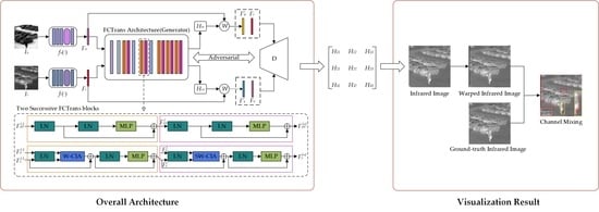
2.1. Overview
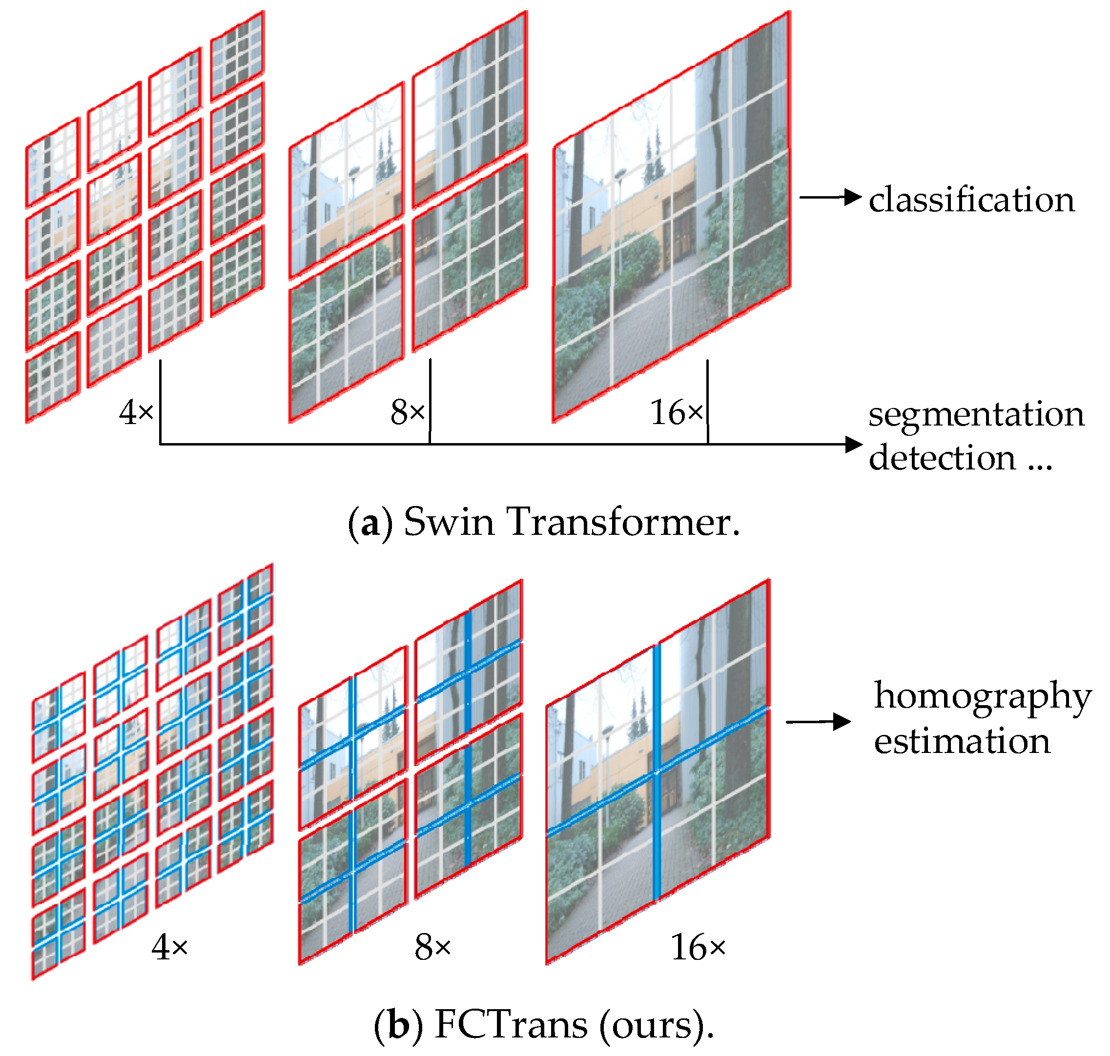
2.2. FCTrans Structure
2.2.1. Feature Patch
| Algorithm 1: The training process of the FCTrans | ||
| Input: | ||
| Output: FCL and homography matrix | ||
| input to the patch partition layer and linear embedding layer: ; | ||
| input to the patch partition layer and linear embedding layer: ; | ||
| ; | ||
| for n < number_of_stages do | ||
| for k < number_of_blocks do | ||
| ; | ||
| ; | ||
| ; | ||
| Select and input to (S)W-CIA module: , ; | ||
| input to LayerNorm layer and MLP: ; | ||
| input to LayerNorm layer and MLP: ; | ||
| Select input to LayerNorm layer and MLP: ; | ||
| ; | ||
| End | ||
| if n < (number_of_stages-1) do | ||
| input to patch merging layer; | ||
| input to patch merging layer; | ||
| input to patch merging layer; | ||
| end | ||
| ; | ||
| ; | ||
| Return: and ; | ||
2.2.2. Cross-Image Attention
2.3. Loss Function
2.3.1. Loss Function of the Generator
2.3.2. Loss Function of the Discriminator
3. Experimental Results
3.1. Dataset
3.2. Implementation Details
3.3. Evaluation Metrics
3.4. Comparison on Synthetic Benchmark Datasets
3.4.1. Qualitative Comparison
3.4.2. Quantitative Comparison
3.5. Comparison on the Real-World Dataset
3.6. Ablation Studies
3.6.1. FCTrans
3.6.2. Feature Patch
3.6.3. Cross-Image Attention
3.6.4. FCL
4. Discussion
5. Conclusions
Author Contributions
Funding
Data Availability Statement
Acknowledgments
Conflicts of Interest
Abbreviations
| 6G SAGIN | 6G Space–Air–Ground Integrated Network |
| SAR | Synthetic Aperture Radar |
| DLT | Direct Linear Transformation |
| FCL | Feature Correlation Loss |
| SIFT | Scale Invariant Feature Transform |
| SURF | Speeded Up Robust Features |
| ORB | Oriented FAST and Rotated BRIEF |
| BRISK | Binary Robust Invariant Scalable Keypoints |
| AKAZE | Accelerated-KAZE |
| LPM | Locality Preserving Matching |
| GMS | Grid-Based Motion Statistics |
| BEBLID | Boosted Efficient Binary Local Image Descriptor |
| LIFT | Learned Invariant Feature Transform |
| SOSNet | Second-Order Similarity Network |
| OAN | Order-Aware Networks |
| RANSAC | Random Sample Consensus |
| MAGSAC | Marginalizing Sample Consensus |
| W-CIA | Cross-image attention with regular window |
| SW-CIA | Cross-image attention with shifted window |
| STN | Spatial Transformation Network |
| Adam | Adaptive Moment Estimation |
Appendix A. Dependency on

| Easy | Moderate | Hard | Average | |
|---|---|---|---|---|
| 0.001 | 4.15 | 5.28 | 6.26 | 5.33 |
| 0.005 | 3.75 | 4.70 | 5.94 | 4.91 |
| 0.01 | 3.83 | 4.88 | 6.06 | 5.03 |
References
- Liao, Z.; Chen, C.; Ju, Y.; He, C.; Jiang, J.; Pei, Q. Multi-Controller Deployment in SDN-Enabled 6G Space–Air–Ground Integrated Network. Remote Sens. 2022, 14, 1076. [Google Scholar] [CrossRef]
- Chen, C.; Wang, C.; Liu, B.; He, C.; Cong, L.; Wan, S. Edge Intelligence Empowered Vehicle Detection and Image Segmentation for Autonomous Vehicles. IEEE Trans. Intell. Transp. Syst. 2023, 1–12. [Google Scholar] [CrossRef]
- Ju, Y.; Chen, Y.; Cao, Z.; Liu, L.; Pei, Q.; Xiao, M.; Ota, K.; Dong, M.; Leung, V.C. Joint Secure Offloading and Resource Allocation for Vehicular Edge Computing Network: A Multi-Agent Deep Reinforcement Learning Approach. IEEE Trans. Intell. Transp. Syst. 2023, 24, 5555–5569. [Google Scholar] [CrossRef]
- Chen, C.; Yao, G.; Liu, L.; Pei, Q.; Song, H.; Dustdar, S. A Cooperative Vehicle-Infrastructure System for Road Hazards Detection With Edge Intelligence. IEEE Trans. Intell. Transp. Syst. 2023, 24, 5186–5198. [Google Scholar] [CrossRef]
- Xu, H.; Ma, J.; Yuan, J.; Le, Z.; Liu, W. Rfnet: Unsupervised network for mutually reinforcing multi-modal image registration and fusion. In Proceedings of the IEEE/CVF Conference on Computer Vision and Pattern Recognition, New Orleans, LA, USA, 19–24 June 2022; pp. 19679–19688. [Google Scholar]
- Li, L.; Han, L.; Ding, M.; Cao, H. Multimodal image fusion framework for end-to-end remote sensing image registration. IEEE Trans. Geosci. Remote Sens. 2023, 61, 1–14. [Google Scholar] [CrossRef]
- LaHaye, N.; Ott, J.; Garay, M.J.; El-Askary, H.M.; Linstead, E. Multi-modal object tracking and image fusion with unsupervised deep learning. IEEE J. Sel. Top. Appl. Earth Observ. Remote Sens. 2019, 12, 3056–3066. [Google Scholar] [CrossRef]
- Zhang, X.; Ye, P.; Leung, H.; Gong, K.; Xiao, G. Object fusion tracking based on visible and infrared images: A comprehensive review. Inf. Fusion 2020, 63, 166–187. [Google Scholar] [CrossRef]
- Lv, N.; Zhang, Z.; Li, C.; Deng, J.; Su, T.; Chen, C.; Zhou, Y. A hybrid-attention semantic segmentation network for remote sensing interpretation in land-use surveillance. Int. J. Mach. Learn. Cybern. 2023, 14, 395–406. [Google Scholar] [CrossRef]
- Drouin, M.A.; Fournier, J. Infrared and Visible Image Registration for Airborne Camera Systems. In Proceedings of the 2022 IEEE International Conference on Image Processing (ICIP), Bordeaux, France, 16–19 October 2022; pp. 951–955. [Google Scholar]
- Jia, F.; Chen, C.; Li, J.; Chen, L.; Li, N. A BUS-aided RSU access scheme based on SDN and evolutionary game in the Internet of Vehicle. Int. J. Commun. Syst. 2022, 35, e3932. [Google Scholar] [CrossRef]
- Shugar, D.H.; Jacquemart, M.; Shean, D.; Bhushan, S.; Upadhyay, K.; Sattar, A.; Schwanghart, W.; Mcbride, S.; Van Wyk de Vries, M.; Mergili, M.; et al. A massive rock and ice avalanche caused the 2021 disaster at Chamoli, Indian Himalaya. Science 2021, 373, 300–306. [Google Scholar] [CrossRef]
- Muhuri, A.; Bhattacharya, A.; Natsuaki, R.; Hirose, A. Glacier surface velocity estimation using stokes vector correlation. In Proceedings of the 2015 IEEE 5th Asia-Pacific Conference on Synthetic Aperture Radar (APSAR), Singapore, 29 October 2015; pp. 606–609. [Google Scholar]
- Schmah, T.; Yourganov, G.; Zemel, R.S.; Hinton, G.E.; Small, S.L.; Strother, S.C. Comparing classification methods for longitudinal fMRI studies. Neural Comput. 2010, 22, 2729–2762. [Google Scholar] [CrossRef] [PubMed]
- Gao, X.; Shi, Y.; Zhu, Q.; Fu, Q.; Wu, Y. Infrared and Visible Image Fusion with Deep Neural Network in Enhanced Flight Vision System. Remote Sens. 2022, 14, 2789. [Google Scholar] [CrossRef]
- Hu, H.; Li, B.; Yang, W.; Wen, C.-Y. A Novel Multispectral Line Segment Matching Method Based on Phase Congruency and Multiple Local Homographies. Remote Sens. 2022, 14, 3857. [Google Scholar] [CrossRef]
- Nie, L.; Lin, C.; Liao, K.; Liu, S.; Zhao, Y. Depth-Aware Multi-Grid Deep Homography Estimation with Contextual Correlation. arXiv 2021, arXiv:2107.02524. [Google Scholar] [CrossRef]
- Li, M.; Liu, J.; Yang, H.; Song, W.; Yu, Z. Structured Light 3D Reconstruction System Based on a Stereo Calibration Plate. Symmetry 2020, 12, 772. [Google Scholar] [CrossRef]
- Hartley, R.; Zisserman, A. Multiple View Geometry in Computer Vision; Cambridge University Press: Cambridge, UK, 2003. [Google Scholar]
- Lowe, D.G. Distinctive image features from scale-invariant keypoints. Int. J. Comput. Vis. 2004, 60, 91–110. [Google Scholar] [CrossRef]
- Bay, H.; Tuytelaars, T.; Gool, L.V. Surf: Speeded Up Robust Features. In Proceedings of the European Conference on Computer Vision, Graz, Austria, 7–13 May 2006; pp. 404–417. [Google Scholar]
- Rublee, E.; Rabaud, V.; Konolige, K.; Bradski, G. ORB: An Efficient Alternative to SIFT or SURF. In Proceedings of the 2011 International Conference on Computer Vision, Barcelona, Spain, 6–13 November 2011; pp. 2564–2571. [Google Scholar]
- Leutenegger, S.; Chli, M.; Siegwart, R.Y. BRISK: Binary Robust Invariant Scalable Keypoints. In Proceedings of the 2011 International Conference on Computer Vision, Barcelona, Spain, 6–13 November 2011; pp. 2548–2555. [Google Scholar]
- Alcantarilla, P.F.; Solutions, T. Fast explicit diffusion for accelerated features in nonlinear scale spaces. IEEE Trans. Patt. Anal. Mach. Intell 2011, 34, 1281–1298. [Google Scholar]
- Alcantarilla, P.F.; Bartoli, A.; Davison, A.J. KAZE Features. In Proceedings of the Computer Vision–ECCV 2012: 12th European Conference on Computer Vision, Florence, Italy, 7–13 October 2012; pp. 214–227. [Google Scholar]
- Ma, J.; Zhao, J.; Jiang, J.; Zhou, H.; Guo, X. Locality preserving matching. Int. J. Comput. Vis. 2019, 127, 512–531. [Google Scholar] [CrossRef]
- Bian, J.W.; Lin, W.Y.; Matsushita, Y.; Yeung, S.K.; Nguyen, T.D.; Cheng, M.M. Gms: Grid-Based Motion Statistics for Fast, Ultra-Robust Feature Correspondence. In Proceedings of the IEEE Conference on Computer Vision and Pattern Recognition, Honolulu, HI, USA, 21–26 July 2017; pp. 4181–4190. [Google Scholar]
- Suárez, I.; Sfeir, G.; Buenaposada, J.M.; Baumela, L. BEBLID: Boosted efficient binary local image descriptor. Pattern Recognit. Lett. 2020, 133, 366–372. [Google Scholar] [CrossRef]
- Yi, K.M.; Trulls, E.; Lepetit, V.; Fua, P. Lift: Learned Invariant Feature Transform. In Proceedings of the Computer Vision–ECCV 2016: 14th European Conference, Amsterdam, The Netherlands, 10–16 October 2016; pp. 467–483. [Google Scholar]
- DeTone, D.; Malisiewicz, T.; Rabinovich, A. Superpoint: Self-Supervised Interest Point Detection and Description. In Proceedings of the IEEE Conference on Computer Vision and Pattern Recognition Workshops, Salt Lake City, UT, USA, 18–22 June 2018; pp. 224–236. [Google Scholar]
- Tian, Y.; Yu, X.; Fan, B.; Wu, F.; Heijnen, H.; Balntas, V. Sosnet: Second Order Similarity Regularization for Local Descriptor Learning. In Proceedings of the IEEE/CVF Conference on Computer Vision and Pattern Recognition, Long Beach, CA, USA, 15–20 June 2019; pp. 11016–11025. [Google Scholar]
- Zhang, J.; Sun, D.; Luo, Z.; Yao, A.; Zhou, L.; Shen, T.; Chen, Y.; Quan, L.; Liao, H. Learning Two-View Correspondences and Geometry Using Order-Aware Network. In Proceedings of the IEEE/CVF International Conference on Computer Vision, Seoul, Republic of Korea, 27 October–2 November 2019; pp. 5845–5854. [Google Scholar]
- Mukherjee, D.; Jonathan Wu, Q.M.; Wang, G. A comparative experimental study of image feature detectors and descriptors. Mach. Vis. Appl. 2015, 26, 443–466. [Google Scholar] [CrossRef]
- Forero, M.G.; Mambuscay, C.L.; Monroy, M.F.; Miranda, S.L.; Méndez, D.; Valencia, M.O.; Gomez Selvaraj, M. Comparative Analysis of Detectors and Feature Descriptors for Multispectral Image Matching in Rice Crops. Plants 2021, 10, 1791. [Google Scholar] [CrossRef] [PubMed]
- Sharma, S.K.; Jain, K.; Shukla, A.K. A Comparative Analysis of Feature Detectors and Descriptors for Image Stitching. Appl. Sci. 2023, 13, 6015. [Google Scholar] [CrossRef]
- Fischler, M.A.; Bolles, R.C. Random sample consensus: A paradigm for model fitting with applications to image analysis and automated cartography. Commun. ACM 1981, 24, 381–395. [Google Scholar] [CrossRef]
- Barath, D.; Matas, J.; Noskova, J. MAGSAC: Marginalizing Sample Consensus. In Proceedings of the IEEE/CVF Conference on Computer Vision and Pattern Recognition, Long Beach, CA, USA, 15–20 June 2019; pp. 10197–10205. [Google Scholar]
- Barath, D.; Noskova, J.; Ivashechkin, M.; Matas, J. MAGSAC++, a Fast, Reliable and Accurate Robust Estimator. In Proceedings of the IEEE/CVF Conference on Computer Vision and Pattern Recognition, Seattle, WA, USA, 14–19 June 2020; pp. 1304–1312. [Google Scholar]
- DeTone, D.; Malisiewicz, T.; Rabinovich, A. Deep image homography estimation. arXiv 2016, arXiv:1606.03798. [Google Scholar]
- Le, H.; Liu, F.; Zhang, S.; Agarwala, A. Deep Homography Estimation for Dynamic Scenes. In Proceedings of the IEEE/CVF Conference on Computer Vision and Pattern Recognition, Seattle, WA, USA, 14–19 June 2020; pp. 7652–7661. [Google Scholar]
- Shao, R.; Wu, G.; Zhou, Y.; Fu, Y.; Fang, L.; Liu, Y. Localtrans: A Multiscale Local Transformer Network for Cross-Resolution Homography Estimation. In Proceedings of the IEEE/CVF International Conference on Computer Vision, Montreal, QC, Canada, 10–17 October 2021; pp. 14890–14899. [Google Scholar]
- Nguyen, T.; Chen, S.W.; Shivakumar, S.S.; Taylor, C.J.; Kumar, V. Unsupervised deep homography: A fast and robust homography estimation model. IEEE Robot. Autom. Lett. 2018, 3, 2346–2353. [Google Scholar] [CrossRef] [Green Version]
- Zhang, J.; Wang, C.; Liu, S.; Jia, L.; Ye, N.; Wang, J.; Zhou, J.; Sun, J. Content-Aware Unsupervised Deep Homography Estimation. In Proceedings of the Computer Vision–ECCV 2020: 16th European Conference, Glasgow, UK, 23–28 August 2020; pp. 653–669. [Google Scholar]
- Ye, N.; Wang, C.; Fan, H.; Liu, S. Motion Basis Learning for Unsupervised Deep Homography Estimation with Subspace Projection. In Proceedings of the IEEE/CVF International Conference on Computer Vision, Montreal, QC, Canada, 10–17 October 2021; pp. 13117–13125. [Google Scholar]
- Hong, M.; Lu, Y.; Ye, N.; Lin, C.; Zhao, Q.; Liu, S. Unsupervised Homography Estimation with Coplanarity-Aware GAN. In Proceedings of the IEEE/CVF Conference on Computer Vision and Pattern Recognition, New Orleans, LA, USA, 19–24 June 2022; pp. 17663–17672. [Google Scholar]
- Luo, Y.; Wang, X.; Wu, Y.; Shu, C. Detail-Aware Deep Homography Estimation for Infrared and Visible Image. Electronics 2022, 11, 4185. [Google Scholar] [CrossRef]
- Luo, Y.; Wang, X.; Wu, Y.; Shu, C. Infrared and Visible Image Homography Estimation Using Multiscale Generative Adversarial Network. Electronics 2023, 12, 788. [Google Scholar] [CrossRef]
- Liu, Z.; Lin, Y.; Cao, Y.; Hu, H.; Wei, Y.; Zhang, Z.; Lin, S.; Guo, B. Swin transformer: Hierarchical vision transformer using shifted windows. In Proceedings of the IEEE/CVF International Conference on Computer Vision, Montreal, QC, Canada, 10–17 October 2021; pp. 10012–10022. [Google Scholar]
- Huo, M.; Zhang, Z.; Yang, X. AbHE: All Attention-based Homography Estimation. arXiv 2022, arXiv:2212.03029. [Google Scholar]
- Jaderberg, M.; Simonyan, K.; Zisserman, A.; Kavukcuoglu, K. Spatial Transformer Networks. In Proceedings of the Advances in Neural Information Processing Systems, Montreal, QC, Canada, 7–12 December 2015; pp. 2017–2025. [Google Scholar]
- Vaswani, A.; Shazeer, N.; Parmar, N.; Uszkoreit, J.; Jones, L.; Gomez, A.N.; Kaiser, L.; Polosukhin, I. Attention Is All You Need. In Advances in Neural Information Processing Systems 30; Massachusetts Institute of Technology: Cambridge, MA, USA, 2017. [Google Scholar]
- Aguilera, C.; Barrera, F.; Lumbreras, F.; Sappa, A.D.; Toledo, R. Multispectral Image Feature Points. Sensors 2012, 12, 12661–12672. [Google Scholar] [CrossRef] [Green Version]
- Kingma, D.P.; Ba, J. Adam: A method for stochastic optimization. arXiv 2014, arXiv:1412.6980. [Google Scholar]


| Parameter | Experimental Environment |
|---|---|
| Operating System | Windows 10 |
| GPU | NVIDIA GeForce RTX 3090 |
| Memory | 64 GB |
| Python | 3.6.13 |
| Deep Learning Framework | Pytorch 1.10.0/CUDA 11.3 |
| Parameter | Value |
|---|---|
| Image Size | |
| Image Patch Size | |
| Initial Learning Rate | 0.0001 |
| Optimizer | Adam |
| Weight Decay | 0.0001 |
| Learning Rate Decay Factor | 0.8 |
| Batch Size | 32 |
| Epoch | 50 |
| Window Size (M) | 16 |
| Feature Patch Size | 2 |
| Channel Number (C) | 18 |
| Block Numbers | {2,2,6} |
| (1) | Method | Easy | Moderate | Hard | Average | Failure Rate |
|---|---|---|---|---|---|---|
| (2) | 4.59 | 5.71 | 6.77 | 5.79 | 0% | |
| (3) | SIFT [20] + RANSAC [36] | 50.87 | Nan | Nan | 50.87 | 93% |
| (4) | SIFT [20] + MAGSAC++ [38] | 131.72 | Nan | Nan | 131.72 | 93% |
| (5) | ORB [22] + RANSAC [36] | 82.64 | 118.29 | 313.74 | 160.89 | 17% |
| (6) | ORB [22] + MAGSAC++ [38] | 85.99 | 109.14 | 142.54 | 109.13 | 19% |
| (7) | BRISAK [23] + RANSAC [36] | 104.06 | 126.8 | 244.01 | 143.2 | 24% |
| (8) | BRISAK [23] +MAGSAC++ [38] | 101.37 | 136.01 | 234.14 | 143.4 | 24% |
| (9) | AKAZE [24] + RANSAC [36] | 99.39 | 230.89 | Nan | 159.66 | 43% |
| (10) | AKAZE [24] + MAGSAC++ [38] | 101.36 | 210.05 | Nan | 139.4 | 52% |
| (11) | CADHN [43] | 4.09 | 5.21 | 6.17 | 5.25 | 0% |
| (12) | DADHN [46] | 3.84 | 5.01 | 6.09 | 5.08 | 0% |
| (13) | HomoMGAN [47] | 3.85 | 4.99 | 6.05 | 5.06 | 0% |
| (14) | Proposed algorithm | 3.75 | 4.70 | 5.94 | 4.91 | 0% |
| (1) | Method | Easy | Moderate | Hard | Average | Failure Rate |
|---|---|---|---|---|---|---|
| (2) | 2.36 | 3.63 | 4.99 | 3.79 | Nan | |
| (3) | SIFT [20] + RANSAC [36] | 135.43 | Nan | Nan | 135.43 | 96% |
| (4) | SIFT [20] + MAGSAC++ [38] | 165.54 | Nan | Nan | 165.54 | 96% |
| (5) | ORB [22] + RANSAC [36] | 40.05 | 63.23 | 159.70 | 76.57 | 22% |
| (6) | ORB [22] + MAGSAC++ [38] | 61.69 | 109.96 | 496.02 | 158.87 | 27% |
| (7) | BRISAK [23] + RANSAC [36] | 44.22 | 81.51 | 483.76 | 151.47 | 24% |
| (8) | BRISAK [23] +MAGSAC++ [38] | 66.09 | 129.58 | 350.06 | 142.75 | 27% |
| (9) | AKAZE [24] + RANSAC [36] | 71.77 | 170.03 | Nan | 83.33 | 66% |
| (10) | AKAZE [24] + MAGSAC++ [38] | 122.64 | Nan | Nan | 122.64 | 71% |
| (11) | CADHN [43] | 2.07 | 3.27 | 4.65 | 3.46 | 0% |
| (12) | DADHN [46] | 2.10 | 3.27 | 4.66 | 3.47 | 0% |
| (13) | HomoMGAN [47] | 2.00 | 3.15 | 4.54 | 3.36 | 0% |
| (14) | Proposed algorithm | 1.69 | 2.55 | 3.79 | 2.79 | 0% |
| (1) | Modification | Easy | Moderate | Hard | Average |
|---|---|---|---|---|---|
| (2) | Change to the Swin Transformer backbone | 4.01 | 5.02 | 6.08 | 5.13 |
| (3) | w/o. feature patch | 3.82 | 4.97 | 5.99 | 5.02 |
| (4) | Change to self-attention and w/o. FCL | 3.96 | 4.96 | 5.91 | 5.03 |
| (5) | w/o. FCL | 3.94 | 5.01 | 6.06 | 5.10 |
| (6) | Proposed algorithm | 3.75 | 4.70 | 5.94 | 4.91 |
Disclaimer/Publisher’s Note: The statements, opinions and data contained in all publications are solely those of the individual author(s) and contributor(s) and not of MDPI and/or the editor(s). MDPI and/or the editor(s) disclaim responsibility for any injury to people or property resulting from any ideas, methods, instructions or products referred to in the content. |
© 2023 by the authors. Licensee MDPI, Basel, Switzerland. This article is an open access article distributed under the terms and conditions of the Creative Commons Attribution (CC BY) license (https://creativecommons.org/licenses/by/4.0/).
Share and Cite
Wang, X.; Luo, Y.; Fu, Q.; Rui, Y.; Shu, C.; Wu, Y.; He, Z.; He, Y. Infrared and Visible Image Homography Estimation Based on Feature Correlation Transformers for Enhanced 6G Space–Air–Ground Integrated Network Perception. Remote Sens. 2023, 15, 3535. https://doi.org/10.3390/rs15143535
Wang X, Luo Y, Fu Q, Rui Y, Shu C, Wu Y, He Z, He Y. Infrared and Visible Image Homography Estimation Based on Feature Correlation Transformers for Enhanced 6G Space–Air–Ground Integrated Network Perception. Remote Sensing. 2023; 15(14):3535. https://doi.org/10.3390/rs15143535
Chicago/Turabian StyleWang, Xingyi, Yinhui Luo, Qiang Fu, Yun Rui, Chang Shu, Yuezhou Wu, Zhige He, and Yuanqing He. 2023. "Infrared and Visible Image Homography Estimation Based on Feature Correlation Transformers for Enhanced 6G Space–Air–Ground Integrated Network Perception" Remote Sensing 15, no. 14: 3535. https://doi.org/10.3390/rs15143535