Technical Note

Long-Range Perception System for Road Boundaries and Objects Detection in Trains

1
Changsha University, 98 Hongshan Road, Changsha 410022, China
2
CRRC Zhuzhou Institute Co., Ltd., 169 Shidai Road, Zhuzhou 412001, China
*
Author to whom correspondence should be addressed.
Remote Sens. 2023, 15(14), 3473; https://doi.org/10.3390/rs15143473
Submission received: 10 March 2023 / Revised: 13 April 2023 / Accepted: 14 April 2023 / Published: 10 July 2023
(This article belongs to the Special Issue Road Detection, Monitoring and Maintenance Using Remotely Sensed Data)

Abstract

:
This article introduces a long-range sensing system based on millimeter-wave radar, which is used to detect the roadside boundaries and track trains for trains. Due to the high speed and long braking distance of trains, existing commercial vehicle sensing solutions cannot meet their needs for long-range target detection. To address this challenge, this study proposes a long-range perception system for detecting road boundaries and trains based on millimeter-wave radar. The system uses high-resolution, long-range millimeter-wave radar customized for the strong scattering environment of rail transit. First, we established a multipath scattering theory in complex scenes such as track tunnels and fences and used the azimuth scattering characteristics to eliminate false detections. A set of accurate calculation methods of the train’s ego-velocity is proposed, which divides the radar detection point clouds into static target point clouds and dynamic target point clouds based on the ego-velocity of the train. We then used the road boundary curvature, global geometric parallel information, and multi-frame information fusion to extract and fit the boundary in the static target point stably. Finally, we performed clustering and shape estimation on the radar track information to identify the train and judge the collision risk based on the position and speed of the detected train and the extracted boundary information. The paper makes a significant contribution by establishing a multipath scattering theory for complex scenes of rail transit to eliminate radar false detection and proposing a train speed estimation strategy and a road boundary feature point extraction method that adapt to the rail environment. As well as building a perception system and installing it on the train for verification, the main line test results showed that the system can reliably detect the road boundary more than 400 m ahead of the train and can stably detect and track the train.

1. Introduction

With the continuous advancement of intelligent technology, intelligent driving systems have been introduced into the field of rail transit to improve the operating efficiency and safety. Environmental perception plays a critical role in intelligent driving and is essential to the safe operation of railways. However, currently, trains primarily rely on automatic blocking technology supported by sophisticated railway communication systems to avoid collisions. This technology keeps trains isolated from each other on different sections of the railway, but it cannot provide accurate information on the position of other trains or detect obstacles on the track ahead. As a result, signal failures or other issues can lead to collisions, as seen in several instances such as the 2013 collision in the Golmud East Section of the Qinghai-Tibet Railway and the 2016 collision in Belgium. Therefore, in addition to advanced railway communication systems, it is also important to equip trains with autonomous perception systems. These systems act as the last line of defense against train collisions and must operate day and night under any weather conditions. They should have a sensing distance greater than the emergency braking distance to ensure safety. By using such systems, rail transit can enhance the operating efficiency and safety, reducing the likelihood of accidents caused by human error or signal failures.

2. Literature Review

Intelligent driving systems have become increasingly common in road traffic, and the technology is maturing. In-vehicle perception sensors are a crucial component of intelligent driving systems and include lidar, millimeter-wave radar, and vision sensors [1,2,3]. While cameras and lidar have limitations under certain weather conditions such as rain, snow, fog, and dense dust, millimeter-wave radar’s robustness under harsh conditions is unmatched [4]. Millimeter-wave radar uses the Doppler effect to detect the speed of obstacles accurately, making it much more accurate than other sensors of the same type. It can also be used for self-attitude and speed estimation [5]. By processing the target points detected by the millimeter-wave radar through clustering [6,7], shape and attitude estimation [8], and boundary fitting [9], information such as the distance, orientation, size, attributes, and collision risk of the target can be obtained. As a result, millimeter-wave radar is widely used in the field of automotive autonomous driving. Given the remarkable performance of millimeter-wave radar in the automotive field, it is anticipated that the detection technology of millimeter-wave radar will further improve the active safety operation capability of rail transit.
The high speed and mass of trains result in long emergency braking distances that necessitate a greater perceived distance for safe operation. This distance is crucial in emergency situations such as signal failures or rockslides blocking railway tracks, where trains must be stopped before colliding. However, current millimeter-wave radar systems used in commercial rail vehicles have a limited resolution and detection range, making it challenging to meet the long-distance target detection needs of trains. Several scientific research teams have conducted research on the application of radar systems in rail transit. For example, roadside millimeter-wave radars are used to detect trains along the line [10]. However, this method faces the same signal failure risks as the railway communication system mentioned above because the millimeter-wave radar is not installed on the train. Another promising development is the K-band long-range radar system proposed by Liu et al., which has the advantage of overcoming angular ambiguity, but its large size and insufficient operating frequency limit its use in mobile platforms [11]. Given the limitations of existing radar systems, there is a need for further research and development of radar detection technology that can meet the long-distance road boundary and target detection needs of trains.
With advancements in radar technology, the latest 4D radar is capable of generating point cloud data similar to lidar, which contains rich Doppler information and has all-weather capabilities [12,13]. The use of multiple-input multiple-output (MIMO) technology and binary phase-shift keying (BPSK) encoding in 4D radar allows for the transmission of signals to obtain elevation information [14], making it useful in applications such as road edge height estimation and drainage manhole cover detection. Additionally, the use of deep learning and artificial intelligence has become widespread in various fields, including target classification research based on millimeter-wave radar [15,16]. While the effectiveness of such research in short-distance areas with dense millimeter-wave radar point clouds is good [17,18,19], it is not ideal in long-distance sparse point clouds. As a result, there is currently a lack of long-range, high-resolution millimeter-wave radars for rail transit applications, along with the associated algorithms for rail transit boundary fitting and boundary-based target detection.
To achieve high-precision detection of long-distance targets by trains, this paper proposes a long-distance perception system based on millimeter-wave radar. The system is designed to detect road boundaries and trains running ahead using a customized set of long-distance, high-resolution millimeter-wave radars suitable for rail transit. Firstly, the paper constructs the theory of multipath scattering in complex scenes such as rail transit tunnels and fences and adopts a method based on azimuth scattering characteristics to further eliminate radar false detections. Secondly, the paper proposes a set of self-running speed calculation methods, which divides the radar detection point cloud into static target point clouds and dynamic target point clouds based on the ego-velocity of the train. Then, the static target point clouds are used to realize the stable extraction and fitting of the road boundary, and all obstacles within the road boundary and other areas of interest are detected, so as to accurately determine whether the perceived target has a collision risk, ultimately improving driving safety. The paper presents several contributions of the proposed system:
(1)
The theory of multipath scattering in complex scenes such as rail transit tunnels and fences is established, and the radar false detections that are stronger or closer to the real point clouds were further eliminated by using the azimuth scattering characteristics.
(2)
To accurately predict possible collisions, a set of ego-velocity estimation strategies of the train is proposed to separate targets with different velocities.
(3)
The system designed in this paper also presents a road boundary feature point extraction and target detection method suitable for rail transit. The proposed methods are capable of detecting road boundaries at a distance greater than 400 m, and the system demonstrated reliable detection of the train ahead.
(4)
A set of high-resolution, long-distance millimeter-wave radar adapted to the rail transit environment was customized, with a detection range of more than 500 m, and it was loaded and operated on the train. The performance of the remote detection system was evaluated using train line operation data collected over a year, covering a variety of scenarios, weather, and speeds.

3. System Framework

The long-distance perception system for trains customizes a train-mounted long-distance, high-resolution millimeter-wave radar as a sensor according to the long-distance perception requirements of rail transit. Figure 1 illustrates the system architecture, which consists of several modules, including the data preprocessing module, speed calculation module, road boundary detection module, and target collision detection module. To begin, the millimeter-wave radar mounted on the train detects environmental point cloud data, which are then transmitted to the data preprocessing module. This module filters out false detections in the data and then sends them to the speed calculation module, where the ego-velocity estimation and separation of moving and static target point clouds take place. Then, the road boundary detection module extracts the boundary feature points in the static target point cloud. Using these boundary points, the road boundary curve of the train is fit to ensure secure transit. The target collision detection module processes the speed and boundary information provided by the speed calculation and road boundary detection modules. The module performs clustering based on spatial position and speed and identifies trains using shape estimation techniques. To assess collision risk, the module evaluates the positional relationship between the detected target and the road boundary. The final perception result is then sent to the intelligent driving system for further processing.

4. Rail Transit Scattering Analysis and False Detection Identification

Rail transit operating environments often have many tunnels, and to ensure the exclusive right of way, the road boundaries are typically isolated by fences. However, when using millimeter-wave radar to detect targets in such environments, the electromagnetic waves will have multiple reflection paths, resulting in radar false detections. This problem is particularly pronounced when there are few objects in the detection environment [20]. In existing studies, methods such as tracking and clustering algorithms have been used to filter out most clutter points effectively [21,22]. However, these methods struggle to filter out radar false detections that are stronger than the real point clouds, and there is a need for a new filtering method. To address this issue, we propose the theory of radar multipath scattering in rail transit environments and studied the difference between the generation mechanism of radar false detection and true detection, as well as their influence on radar boundary detection. This approach prevents radar false detection points from interfering with boundary and target detection.
Radar electromagnetic scattering can be divided into single reflection and multiple reflections in closed spaces such as tunnels [23,24]. Multiple reflections can lead to false detections. 
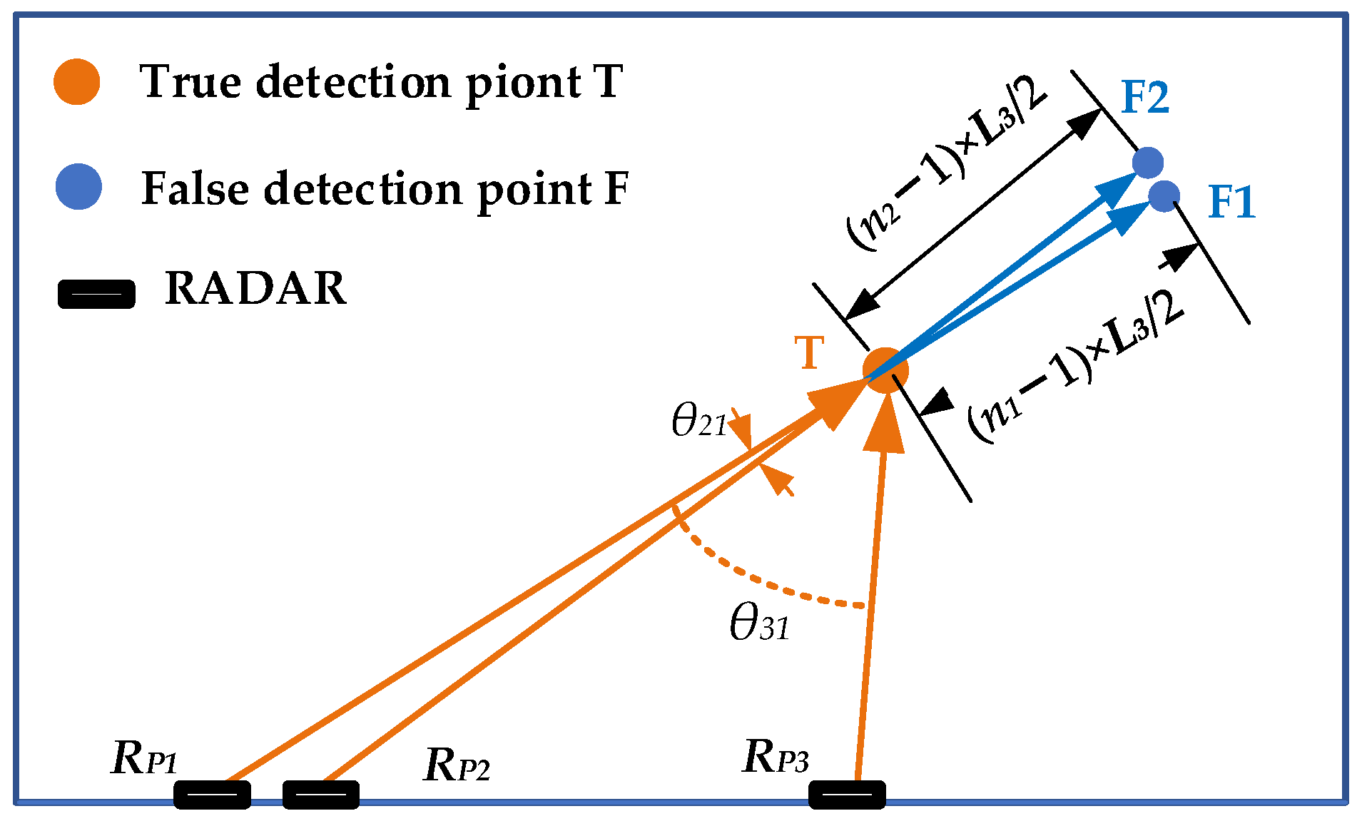
Figure 2 shows a typical scattering path formed by the target and the plane of the tunnel or metal guardrail, resulting in a similar dihedral reflection situation. Single-bounce scattering occurs when the transmitting and receiving path is L1L1, as shown by the black path in the figure. The detection range of a single reflection of the target is L1. However, in the case of two or more reflections, the transmitting and receiving path is L2n × L3L4, where n is the number of reflections between the target and the plane of the tunnel or metal guardrail. The detection distance of two or more reflections of the target can be calculated using the following equation.
L m o r e = L 2 + n × L 3 + L 4 2 = 2 × L 5 + n 1 × L 3 2 = L 5 + n 1 × L 3 / 2 ,     n = 1 ,   3 ,   5
where (n − 1) × L3/2 is the additional deviation distance caused by multiple reflections, which makes the radar detect false point clouds.
Figure 3 shows the difference in the radar point cloud detected by the same target during the radar movement from RP1 to RP3. The assumption was made that the radar detects the real position T of the target at RP1 for the first time and the false detection position F1 of the target for the first time. Furthermore, the radar detects the real position T of the target at the RP2 position and the false detection position F2 that the target is detected for the last time. Finally, the radar detects the real location T of the target at the RP3 position for the last time. It can be seen from Equation (1) that the false detection distance is longer than the real distance in the direction of the radar. Moreover, the false detections cannot overlap together like the T point. These false detections can interfere with the extraction of road boundary feature points and target detection, especially the impact on the seed points used during the road boundary feature point extraction process.
The azimuth scattering angle is a range within which the radar can detect a target [25]. As shown in Figure 3, the azimuth scattering angle of the false detection point is denoted as θ21, while the azimuth scattering angle of the real target point is denoted as θ31. In the rail transit scene, it was observed that the azimuth scattering angle range of the real point is greater than zero. For instance, the convex surface formed by the car body and the horizontal wall in Figure 2 can be regarded as a typical dihedral angle, which can be observed within the azimuth range covered by our radar. However, the azimuth scattering angle range θ21 of false detection points is 0 or very close to 0. This indicates that there is a significant difference in the azimuth scattering angle between the false detection point and the real detection point. It is important to note that the points filtered out by this method are not all false detection points [25]. For example, some points could be caused by the angular accuracy measurement error of the radar itself, while others may be related to the environmental field of view [26].
Therefore, instead of blindly filtering out these points, it is necessary to dynamically adjust the threshold of azimuth filtering false detection points based on the point cloud distribution characteristics. By doing so, we can retain more reliable radar detection points while still filtering out false detections. This approach can lead to an increase in point cloud density, which can further reduce the errors in the process of road boundary detection and target perception.

5. Ego-Velocity Calculation and Separation of Dynamic and Static Targets

The study conducted by Cho et al. used frequency-modulated continuous wave (FMCW) scanning radar to achieve accurate motion estimation alone. However, their approach did not account for interference scenarios where a large number of moving targets exist at the same speed, such as when a long train passes by an adjacent track [5].
To address this limitation, we propose a new method for calculating ego-velocity for rail transit. This method can distinguish dynamic objects from static environment objects based on their ego-velocity. The target velocity detected by the millimeter-wave radar is typically the radial velocity of the target relative to the radar, which is the velocity in the direction of the line between the radar and the target, as shown in Figure 4.
As shown in Figure 4, assuming that the relative ground velocity of the object is  v i  and the angle between  v i  and the radial direction of the radar is  θ i , then the radial velocity of the radar, denoted as  v i , can be calculated:
v i = v i cos θ i
Similarly, assuming that the relative ground velocity of the train is  v t r a i n  and the angle between  v t r a i n  and the radar radial direction is  α i , then the radial velocity of the radar  v t r a i n i  can be calculated:
v t r a i n i = v t r a i n cos α i
From the addition of the relative velocity vectors in the radial direction, we can know the measured velocity  v m e a s u r e i  of the radar to a certain target:
v m e a s u r e i = v i v t r a i n i
When the object detected by the train is a stationary object,    v i  is 0, that is  v i  is 0, and Equation (1) can be simplified as:
v m e a s u r e i = v t r a i n i
From Equations (2) and (4), it can be obtained that the train speed  v t r a i n i  can be calculated by the i-th target:
v t r a i n i = v m e a s u r e i / cos α i
Therefore, in order to determine the ego-velocity of a train, it is necessary to obtain the radar measurement speed of the stationary object and the angle  α i  between the direction of the line between the stationary object and the radar and the normal direction of the radar emitting surface. This angle  α i  is the angle between  v t r a i n  and the radial direction of the radar mentioned above. For all static obstacles, the  v t r a i n i  calculated by Equation (6) should be equal. However, due to measurement errors, the calculated  v t r a i n i  may fluctuate within a certain threshold in actual scenarios. In the context of rail traffic scenarios, most of the obstacles that the radar can detect are static obstacles in most scenarios. To obtain the velocity at which the maximum number of radar point clouds have the same velocity, the mode is used. Ideally, all radar points reflected by the same object should have the same magnitude and direction of velocity. However, in practical scenarios, measurement errors can lead to slight differences in velocity even for multiple radar points reflected by the same object. Hence, the process of finding the mode speed is divided into three steps when the current vehicle speed is unknown. Firstly, all radar points are sorted in ascending order of speed. Secondly, starting from the radar reflection point with the minimum speed, radar points within the range of v0 + delta_v are obtained using delta_v as the threshold. The average speed vi of these radar points is then computed, and new radar points are searched within the range of vi + delta_v. This process is repeated until all radar point clouds have been traversed. All previously found radar points are recorded and stored in set Mi, along with the number of points ki. Finally, the set with the largest ki is identified, and the average speed in the set is taken as the mode speed. Therefore, the simplest way to calculate the train speed is to find the mode of all speeds  v t r a i n i  of all targets calculated by Equation (6). The result obtained after taking the mode is the train’s speed, as shown in Equation (7).
v t r a i n = m o d e v t r a i n i
Although the principles mentioned above are generally reliable for determining the ego-velocity of a train, there are exceptions in the rail transit scenario. For example, when a train passes by an adjacent track, the reflection points detected on one side of the radar field of view all come from this passing train at the same speed. In this case, it is possible that the number of radar points reflected by this passing train exceeds half of all detected radar points, so that the points reflected by this passing train may be mistaken for stationary points. This can lead to inaccuracies in the calculation of the train speed obtained by taking the mode.
To avoid the issues mentioned above and improve the accuracy of the calculated train speed, there are two approaches that can be taken. The first approach is to filter out certain areas to reduce the impact of dynamic obstacles on the results. According to the characteristics of the rail transit scenarios, relatively large dynamic obstacles are mainly trains on adjacent tracks. Thus, to ensure that most of the candidate points are stationary points, points in the adjacent track area can be filtered out based on specific rules before taking the mode of the velocity of the obstacle reflection point. In this regard, a relatively simple filtering rule can be adopted based on the small field of view of the radar and the large radius of curvature of the track. Assuming that the front of the radar is the direction of the x-axis of the coordinate system and the left of the radar is the direction of the y-axis, all points within the range of  y 1 y 2  and  y 3 y 4  on both sides of the radar can be filtered out according to the rules. Here,  y 1 y 2  is the area including the adjacent track on the right and  y 3 y 4  is the area including the adjacent track on the left (the left side of the positive line is generally a fence). The condition  y 1 < y 2 < 0 < y 3 < y 4  should be satisfied. By reasonably setting the parameters to select candidate points, the best results can be obtained.
The second approach to avoid mismeasurement of ego-velocity is based on the continuity assumption of the train’s ego-velocity. The false detection of ego-velocity occurs when most candidate points change from stationary points to detected moving train points on adjacent tracks within a certain period of time. To exclude the influence of moving train points on adjacent tracks, the static target candidate points of each frame can be screened again, assuming that the rail vehicle speed  v t r a i n  changes relatively steadily for a period of time. When the speed of the rail vehicle does not change suddenly, the speed of the stationary obstacle does not change suddenly, then the speed of the stationary targets in the next frame should be within the range of  v t r a i n ± Δ v . Obstacles outside this speed range can be filtered out, ensuring that the majority of candidate points in each frame are static points.
The specific steps of the speed measurement algorithm are shown in Figure 5:
The two steps of area filtering and speed filtering can ensure the accuracy of the radar’s ego-velocity detection effectively. After the train’s speed is obtained, the moving target and the stationary target can be separated according to the train’s speed.

6. Road Boundary Detection and Collision Warning

6.1. Extraction and Fitting of Road Boundary Feature Points

After realizing the separation of the moving target point and the static target point, the road boundary points can be extracted from the static target point. These boundary points are the reflection points of objects detected by the radar with certain regular distribution, such as guardrails, and are roughly distributed on the left and right parallel curves in the radar image. Therefore, the road boundary points can be extracted through the distribution characteristics of the boundary points. To extract these road boundary points, a two-step process is followed:
(1)
Multi-frame radar data superposition: In order to improve the amount of data and reduce the missed detection rate of millimeter-wave radar, it is essential to superimpose continuous multi-frame radar data. The process of superimposing data increases the point density, which is important for accurate detection. Selecting the appropriate number of frames for continuous superimposition is crucial as it affects the overall performance of the system. The number of frames to be superimposed should be selected based on the number of radar point clouds returned per frame and the search threshold of seeds. If the number of superimposed frames is too small, the point density after superimposition will not be enough, whereas selecting too many frames will not significantly improve the results, but will increase the computational cost. Based on our experience with real vehicle testing, we selected six overlapping frames.
(2)
Boundary feature point extraction: According to the longitudinal distance (that is, the forward direction of the train), the target points are traversed from near to far, as the seed point set  A = A 1 , A 2 , , A n , where  A i = x i , y i . According to the abscissa of the seed point, it is divided into left seed point set  A L  and right seed point set  A R , which are processed separately (for the convenience of description, left and right are not distinguished for the time being). Let  Z i 1  be the first starting point of seed point  A i , and let  Z i j  be the j-th starting point. Using each  Z i j  as a starting point, search for other target points  B j = B j 1 , , B j n  within the fan-shaped area in the longitudinal direction a few meters ahead. If there are more than one other target point, the average coordinate point  B j a v e r a g e = x j a v e r a g e , y j a v e r a g e  of one or more target points is used as the next starting point  Z i j + 1 = B j a v e r a g e , until no other obstacle points can be found, forming a point set  Z i = Z i 1 , , Z i n , wherein the direction of the center line of the fan-shaped area corresponding to the first starting point  Z i 1  is along the direction of train travel and the direction of the center line of the fan-shaped area corresponding to the j + 1-th starting point  Z i j + 1  is the direction of the line from  Z i j  to  Z i j + 1 . After the traversal, the point set  Z L  and  Z R  composed of several groups of candidate point sets on the left and right can be obtained. The point set with the largest number of points is selected from the left and right point sets, respectively. For example, the p-th point set in the left point set is used as the left feature point set  Z L p , and the q-th point set in the right point set is used as the right feature point set  Z R q . Based on the spatial characteristics of these two sets of feature point sets, the extracted points should roughly be in two columns on the left and right. In the rail traffic scenario, only the fence points usually meet the conditions among the targets arranged in two rows that can be detected by the millimeter-wave radar. Therefore, this step can extract boundary points. After extracting the boundary points in the rail transit scene, curve fitting can be performed according to the feature point sets distributed in the left and right columns to obtain the boundary of the drivable area in front of the train.

6.2. Train Detection and Recognition

The density-based spatial clustering of applications with noise (DBSCAN) method is commonly used to group millimeter-wave radar detection target points with similar speed, distance, and angle into the same cluster. However, it is primarily utilized in road scenes [6,7]. To account for the unique characteristics of the rail transit environment, modifications have been made to DBSCAN in two aspects. First of all, given that the train points detected by the millimeter-wave radar are mainly arranged along the longitudinal direction (i.e., the x direction), the distance between detection points of the same obstacle in the x direction will be comparatively large, while the y direction will be denser. As a result, different weights (a and b) are assigned in the x and y directions, respectively, as shown in Formula (8):
D i s t i j = a ( x i x j ) 2 + b ( y i y j ) 2
The weights are adjusted such that a < b. In this case,  D i s t i j  will be more influenced by the distance in the y direction than in the x direction, which is also consistent with the difference of the obstacle reflection point in the x and y directions.
In addition to using the Euclidean distance in space as a distance criterion, the “distance”  D i s t _ v i j  in the velocity dimension can also be used as a distance criterion to distinguish objects with similar spatial distances, but different speeds. Here, the obstacle point  P i  can be expressed as  P i x i , y i , v x i , v y i .
Similarly, we took into account the difference between the radar speed measurement in the x and the y directions by adding weights c and d, respectively.
D i s t _ v i j = c ( v x i v x j ) 2 + d ( v y i v y j ) 2
In practice, the accuracy of radar speed measurements in the x direction is typically higher than in the y direction. Therefore, when testing, only the speed in the x direction is considered.
Introducing the weights and the neighborhood distance of the speed dimension, the DBSCAN algorithm can effectively separate different obstacles at numerous target points, including the trains, which require further identification.
Based on the clustered shape estimation, speed characteristics, and the positional relationship between the target and the boundary, it is comprehensively judges whether the target is a train. For instance, when an opposing train is running straight, it is generally represented as a group of points distributed longitudinally along the x direction in the radar image. When driving on a curve, the distribution of train points is a group of points with a small degree of curvature, roughly distributed along the y direction due to the track’s large radius of curvature. The width from the bounding border in the x direction is approximately half the width of the left and right bounding lines. Additionally, the shape features of the point cloud returned by the train can distinguish it from other obstacles. In this study, the bounding box algorithm is employed to estimate the shape of a group of cluster points to obtain a rectangle [8], and the aspect ratio of the rectangle is used to determine whether the target is a train.

6.3. Collision Warning

In rail traffic scenarios, the distance between the track and the road boundary usually falls within a certain range of values. After identifying the opposite train, the distance from the train point to the boundary fence can be determined by calculating the distance from cluster points  P i x i , y i  belonging to the opposite train to the road boundary. Typically, the distance from the oncoming train to the left boundary is calculated because the right boundary may be occluded when the object comes to the train. If the calculated distance is longer than a certain value, it can be considered that the train point does not invade the track where the rail vehicle is located. In addition, trains on the main line all run on the left side. Therefore, if the speed of the detected train is opposite that of the ego-train, it can be inferred that it has not invaded the track where the ego-train is located, indicating that the travel of both trains is safe.

7. Results and Discussions

7.1. Experimental Equipment

The experimental equipment comprises data acquisition and processing equipment. The following will focus on the millimeter-wave radar used for data acquisition. The existing rail-vehicle-mounted millimeter-wave radar is primarily designed for road scenes and faces challenges in rail transit scenarios such as a short detection distance, low azimuth resolution, and poor anti-interference ability, which do not meet the application needs. To address these challenges, a custom MIMO radar for rail transit operating at a frequency of 77 GHz and using four AWR2243 chip cascaded MIMO array radars produced by TI was designed in this paper, enabling the simultaneous transmission of signals by 12 transmission channels [27]. The echo corresponding to the transmitted signal is separated from the 16 receiving channels, providing high azimuth resolution and long detection distance. Additionally, the radar has the capabilities of distance, direction, and speed measurement, meeting the high detection distance requirements of trains. As the track road has a small slope, the angle that needs to be covered in the pitch angle is small. Therefore, the 3 dB beam coverage angle in the pitch direction is reduced, which increases the antenna gain, further increasing the radar’s detection range. Figure 6 depicts the physical image of the customized millimeter-wave radar installed in front of the train, positioned 1.3 m away from the track. The millimeter-wave radar’s detection range exceeds 500 m, with a distance resolution of 1.2 m, an azimuth angle resolution of 0.6°, and an azimuth angle measurement accuracy of 0.1°, as shown in Table 1.

7.2. Experiments and Analysis

To evaluate the performance of our proposed perception system, we conducted experimental verifications of each module function in actual rail transit operation scenarios. The perception system has been installed on trains for testing since September 2021, and data have been collected on the main line of the railway between Shenchi South Station in Xinzhou City, Shanxi Province, China, and Shenmu North Station in Yulin City, Shaanxi Province, China. Additionally, we tested the all-weather capability of the system by selecting the night scene for verification. Our results, as shown in Figure 7, demonstrated that our proposed system effectively extracts the boundary fence of the rail transit environment.
Figure 7a shows the boundary fitting effect of the open-air straight road scene, where the red line segment is the fit boundary curve, and the left and right boundary fitting distance can exceed 400 m. However, in the open-air curve scene (Figure 7b), as the train turns to the left, the boundary on the left side of the train is severely occluded, which results in a greater impact on the fitting of the left boundary. Although the boundary curve fit on the right side can also judge whether there is a collision risk with the front train within a certain distance, it is still difficult for the system to meet the perceived distance requirement when the turning radius is small. In the tunnel scene (Figure 7c), the current fitting distance is within 200 m, due to the significant impact of multipath in closed scenes. It can be observed that, in curves and tunnel scenarios, the perception system faces challenges in meeting the needs of trains for long-distance perception.
Since rail transit belongs to the exclusive right of way, the main goal of our perception system is to prevent train collisions, focusing on the system’s long-distance detection and speed measurement capabilities for trains. Figure 8a shows the scene when there is an oncoming train. The rail vehicle is driving on the left, and the oncoming rail vehicle is coming from the right. As shown in Figure 8b, our system can effectively detect the speed, position, and shape of the opposite train through algorithms such as speed calculation, clustering, and shape estimation. The yellow dots represent the detected trains. Therefore, it can be determined whether there is a risk of collision based on the distance between the oncoming vehicle and the left and right boundaries. In addition, on the main line, the trains all run on the left, so judging the direction of the train through the speed can also determine whether it is the same train or the opposite train. If it is a train traveling in the same direction, the collision risk is judged based on the distance and speed. The red curves in the figure represent the fitted road boundaries, and the yellow circles represent the detected trains.

7.3. Results and Analysis

When the train is running on the main line, the main detection object is the train. This paper investigated the detection ability of the proposed system for the characteristics of a train target, such as its position and velocity.
Figure 9a shows that the system accurately calculates the speed of the train, which is validated by the agreement between the black curve representing the train’s ego-velocity given by the Global Navigation Satellite Systems (GNSS) + real-time kinematic (RTK) and the red curve representing the rail vehicle speed calculated by the proposed system. The blue curve represents the oncoming train target detected by the system, and it is relatively stable and in line with the speed law of train operation, indicating the accuracy of the system’s speed measurement. In Figure 9b, the black curve represents the distance from the oncoming train detected by the system to the radar, and the red curve represents the distance from the head of the oncoming train detected by the system to the left boundary of the road. The system can detect moving trains up to 400 m away, and it can detect and track stably. In addition, the detected fluctuation of the distance from the head of the oncoming train to the left boundary line of the road is within plus or minus 1.5 m, which is suitable for judging the positional relationship between the train and the boundary. It can be seen that the system is stable for moving train and boundary detection.
The detection stability of static trains within the bounds was analyzed next. The coordinate system was established with the forward direction of the train as the positive direction of the x-axis and the left side of the train as the positive direction of the y-axis. By combining with the Universal Transverse Mercator (UTM) coordinates of the radar given by the GNSS + TRK system and the relative position of the detected train and the radar, the UTM coordinates of the detected train can be obtained. Since the target is stationary, the mean value of the statistic is used as the true value of its UTM coordinate. The error calculation equation of position coordinates (east, north) is as follows:
x i _ position error = x i i = 1 n x i n
y i _ position error = y i i = 1 n y i n
In the formula: i = 1~n, which is the measurement value of a single frame sample; n is the total number of frames;  x i  and  y i  are the coordinates of i in the east and north of the coordinate system, respectively, and the unit is m. As shown in Figure 10a, the red curve represents the distance from the radar to the detected static train, and the blue curve represents the detection effect of the proposed system on the train target. “1” indicates that a static train has been detected, and “0” indicates that it has not been detected. The system can detect stationary trains up to 400 m away, and as many as 18 frames were missed among the 300 frames of data. However, the system detected a total of 235 frames without losing a single frame within 345 m from the train, indicating the stability of the detection of static trains. In Figure 10b, the black curve represents the speed of the train when it approaches the target, and the red and blue curves represent the position coordinate error of each frame measurement value. The accuracy of the system for static train position detection was validated by the maximum error values of the x (east) and y (north) position coordinates, which are both less than 2 m when the train is in motion.
To ensure safety between trains, we calculated the required safe distance between them based on the maximum running speed of the train and the braking rate of the full-load downhill situation. Our analysis revealed that when the train speed is below 90 km/h (25 m/s) and the emergency braking rate a of the train can reach 0.8 m/s2, the required safety distance between trains is greater than s = v2/2a = 390.625 m. As the detection distance of the system we designed is 400 m, it can effectively meet the perception distance requirement of ordinary trains. However, with increasing train speed, the required safety distance between trains also increases. For instance, when the train speed reaches 160 km/h, the emergency braking distance under the same emergency braking rate will exceed 1200 m. Therefore, it is necessary to develop a longer-distance perception system to meet the perception needs of high-speed trains.
Although the proposed system has a good boundary and train detection effect, there are still some challenges to be addressed. For example, when a train enters a station with multiple lanes, the perception system cannot judge the positional relationship between the lane the rail vehicle will travel on and the detected target, which prevents it from performing collision risk analysis. To overcome this challenge, it is necessary to combine positioning and map prior information to obtain the specific location of the road ahead for collision analysis.

8. Conclusions

This paper presented a theory of multipath scattering in complex scenes such as rail transit tunnels and fences, which was used to eliminate radar false detection points that are stronger or closer to the real point cloud. The paper proposed a set of strategies for ego-velocity calculation to separate objects with different speeds and also proposed a set of road boundary feature point extraction and object detection methods suitable for rail transit. Experimental tests conducted in actual rail transit scenes demonstrated that the proposed system can accurately detect dynamic trains beyond a distance of 400 m and fit road boundary lengths over 400 m. To further extend the detection range of the system, the challenge lies not in enhancing the range of the millimeter-wave radar, but in areas where there are no prominent road boundary features such as regular fences and poles, such as at stations, three-way intersections, and shunting lanes. Consequently, the system may not be able to detect the effective road boundary ahead of the train, leading to an inability to evaluate collision risks by analyzing the road boundary ahead of the train. To overcome this limitation, future research will focus on positioning and mapping technology to develop a high-precision three-dimensional road map. By combining the map’s prior information with the train’s running route’s prior information, a virtual road boundary can be created in front of the train, enabling precise analysis of collision risks.

Author Contributions

Conceptualization, X.F., W.P., H.L. and K.H.; methodology, W.P.; software, H.L.; validation, X.F., W.P. and H.L.; formal analysis, W.P.; investigation, X.F. and K.H.; data curation, H.L.; writing—original draft preparation, X.F. and W.P.; writing—review and editing, H.L. and K.H.; visualization, H.L. and K.H. All authors have read and agreed to the published version of the manuscript.

Funding

This work was supported by National Natural Science Foundation of China (5210120159) and the Talent Introduction Research Foundation of Changsha University (SF2149).

Data Availability Statement

Not applicable.

Acknowledgments

All authors would like to thank the Editors and anonymous Reviewers for their valuable comments and suggestions, which improved the quality of the manuscript.

Conflicts of Interest

The authors declare no conflict of interest.

References

  1. Van Brummelen, J.; O’Brien, M.; Gruyer, D.; Najjaran, H. Autonomous vehicle perception: The technology of today and tomorrow. Transp. Res. Part C Emerg. Technol. 2018, 89, 384–406. [Google Scholar] [CrossRef]
  2. Li, Y.; Ibanez-Guzman, J. Lidar for autonomous driving: The principles, challenges, and trends for automotive lidar and perception systems. IEEE Signal Process. Mag. 2020, 37, 50–61. [Google Scholar] [CrossRef]
  3. Liu, H.; Pan, W.; Hu, Y.; Li, C.; Yuan, X.; Long, T. A Detection and Tracking Method Based on Heterogeneous Multi-Sensor Fusion for Unmanned Mining Trucks. Sensors 2022, 22, 5989. [Google Scholar] [CrossRef] [PubMed]
  4. Lee, S.; Yoon, Y.-J.; Lee, J.-E.; Kim, S.-C. Human–vehicle classification using feature-based SVM in 77-GHz automotive FMCW radar. IET Radar Sonar Navig. 2017, 11, 1589–1596. [Google Scholar] [CrossRef]
  5. Cho, H.; Choi, S.; Cho, Y.; Kim, J. Deep complex-valued network for ego-velocity estimation with millimeter-wave radar. In Proceedings of the 2020 IEEE SENSORS, Shanghai, China, 6–9 November 2020; pp. 1–4. [Google Scholar]
  6. Wagner, T.; Feger, R.; Stelzer, A. Modification of DBSCAN and application to range/Doppler/DoA measurements for pedestrian recognition with an automotive radar system. In Proceedings of the 2015 European Radar Conference (EuRAD), Paris, France, 8–10 September 2015; pp. 269–272. [Google Scholar]
  7. Lim, S.; Lee, S.; Kim, S. Clustering of detected targets using DBSCAN in automotive radar systems. In Proceedings of the 2018 19th International Radar Symposium (IRS), Bonn, Germany, 20–22 June 2018; pp. 1–7. [Google Scholar]
  8. Schlichenmaier, J.; Selvaraj, N.; Stolz, M.; Waldschmidt, C. Template matching for radar-based orientation and position estimation in automotive scenarios. In Proceedings of the 2017 IEEE MTT-S International Conference on Microwaves for Intelligent Mobility (ICMIM), Nagoya, Japan, 19–21 March 2017; pp. 95–98. [Google Scholar]
  9. Kim, T.; Song, B. Detection and Tracking of Road Barrier Based on Radar and Vision Sensor Fusion. J. Sens. 2016, 10, 1963450. [Google Scholar] [CrossRef] [Green Version]
  10. India Company Invented Collision Avoidance Radar System to Make Trains Travel Safer. 2010. Available online: http://www.chinanews.com/shipin/2010/12-21/news30667.html (accessed on 22 November 2022).
  11. Liu, A.; Yang, Q.; Zhang, X.; Deng, W. Collision Avoidance Radar System for the Bullet Train: Implementation and First Results. IEEE Aerosp. Electron. Syst. Mag. 2017, 32, 4–17. [Google Scholar] [CrossRef]
  12. Brisken, S.; Ruf, F.; Höhne, F. Recent evolution of automotive imaging radar and its information content. IET Radar Sonar Navig. 2018, 12, 1078–1081. [Google Scholar] [CrossRef]
  13. Li, G.; Sit, Y.L.; Manchala, S.; Kettner, T.; Ossowska, A.; Krupinski, K.; Sturm, C.; Lubbert, U. Novel 4D 79 GHz Radar Concept for Object Detection and Active Safety Applications. In Proceedings of the 2019 12th German Microwave Conference (GeMiC), Stuttgart, Germany, 25–27 March 2019; pp. 87–90. [Google Scholar]
  14. Stolz, M.; Wolf, M.; Meinl, F.; Kunert, M.; Menzel, W. A New Antenna Array and Signal Processing Concept for an Automotive 4D Radar. In Proceedings of the 2018 15th European Radar Conference (EuRAD), Madrid, Spain, 26–28 September 2018; pp. 63–66. [Google Scholar]
  15. Chen, X.; Ma, H.; Wan, J.; Li, B.; Xia, T. Multi-view 3D Object Detection Network for Autonomous Driving. In Proceedings of the 2017 IEEE Conference on Computer Vision and Pattern Recognition (CVPR), Honolulu, HI, USA, 21–26 July 2017; pp. 6526–6534. [Google Scholar]
  16. Guo, M.; Cai, J.; Liu, Z.; Mu, T.; Martin, R.R.; Hu, S. PCT: Point cloud transformer. Comput. Vis. Media 2021, 7, 187–199. [Google Scholar] [CrossRef]
  17. Bai, J.; Zheng, L.; Li, S.; Tan, B.; Chen, S.; Huang, L. Radar transformer: An object classification network based on 4D MMW imaging radar. Sensors 2021, 21, 3854. [Google Scholar] [CrossRef] [PubMed]
  18. Abdu, F.J.; Zhang, Y.; Fu, M.; Li, Y.; Deng, Z. Application of Deep Learning on Millimeter-Wave Radar Signals: A Review. Sensors 2021, 21, 1951. [Google Scholar] [CrossRef] [PubMed]
  19. Brodeski, D.; Bilik, I.; Giryes, I. Deep radar detector. In Proceedings of the 2019 IEEE Radar Conference (RadarConf), Boston, MA, USA, 22–26 April 2019; pp. 1–6. [Google Scholar]
  20. Witrisal, K.; Meissner, P.; Leitinger, E.; Shen, Y.; Gustafson, C.; Tufvesson, F.; Haneda, K.; Dardari, D.; Molisch, A.F.; Conti, A.; et al. High-Accuracy Localization for Assisted Living: 5G systems will turn multipath channels from foe to friend. IEEE Signal Process. Mag. 2016, 33, 59–70. [Google Scholar] [CrossRef]
  21. Guo, X.P.; Du, J.S.; Gao, J.; Wang, W. Pedestrian Detection Based on Fusion of Millimeter Wave Radar and Vision. In Proceedings of the 2018 International Conference on Intelligence and Pattern Recognition, Beijing, China, 18–20 August 2018; pp. 38–42. [Google Scholar]
  22. Kellner, D.; Klappstein, J.; Dietmayer, K. Grid-based DBSCAN for clustering extended objects in radar data. In Proceedings of the Intelligent Vehicles Symposium, Madrid, Spain, 3–7 June 2012; pp. 365–370. [Google Scholar]
  23. Etinger, A.; Litvak, B.; Pinhasi, Y. Multi Ray Model for Near-Ground Millimeter Wave Radar. Sensors 2017, 17, 1983. [Google Scholar] [CrossRef] [PubMed] [Green Version]
  24. Pan, W.; Huang, C.; Chen, P.; Ma, X.; Hu, C.; Luo, X. A low-RCS and high-gain partially reflecting surface antenna. IEEE Trans. Antennas Propag. 2013, 62, 945–949. [Google Scholar] [CrossRef]
  25. Li, Y.; Wei, Y.; Wang, Y.; Lin, Y.; Shen, W.; Jiang, W. False Detections Revising Algorithm for Millimeter Wave Radar SLAM in Tunnel. Remote Sens. 2023, 15, 277. [Google Scholar] [CrossRef]
  26. Paredes, J.A.; Alvarez, F.J.; Hansard, M.; Rajab, K.Z. A Gaussian Process model for UAV localization using millimetre wave radar. Expert Syst. Appl. 2021, 185, 13. [Google Scholar] [CrossRef]
  27. Design Guide: TIDEP-01012—Imaging Radar Using Cascaded mmWave Sensor Reference Design (REV. A). Available online: http://www.ti.com/lit/ug/tiduen5a/tiduen5a.pdf (accessed on 2 January 2023).
Figure 1. Train detection system framework.
Remotesensing 15 03473 g001
Figure 2. Scattering paths for a typical scene.
Remotesensing 15 03473 g002
Figure 3. False detection points in different positions.
Remotesensing 15 03473 g003
Figure 4. Radical velocity diagram.
Remotesensing 15 03473 g004
Figure 5. Ego-velocity calculation algorithm diagram.
Remotesensing 15 03473 g005
Figure 6. The physical picture of the millimeter-wave radar installed on the rail vehicle.
Remotesensing 15 03473 g006
Figure 7. (a) Fitting effect of straight road boundary in open-air scene; (b) fitting effect of curve road boundary in open-air scene; (c) fitting effect of tunnel scene boundary.
Remotesensing 15 03473 g007
Figure 8. (a) Oncoming car scene in open-air scene; (b) train detection effect.
Remotesensing 15 03473 g008
Figure 9. Detection and tracking effect of the oncoming train: (a) velocity of the train and oncoming train; (b) detection accuracy of the distance from the train to the boundary.
Remotesensing 15 03473 g009
Figure 10. Detection and tracking effect of the stationary train: (a) detection stability and distance; (b) speed and position coordinates error.
Remotesensing 15 03473 g010
Table 1. Key parameters of millimeter wave radar.
ParameterSpecificationsDescription
Maximum Range500 mThe radar can detect an object representing an RCS of approximately 10 m2.
Range Resolution120 cmDistinguish between two or more targets on the same bearing, but at different ranges.
Azimuth Angle Resolution0.6°Distinguish between two or more targets with the same range and velocity, but different angles.
Azimuth Angle Measurement Accuracy0.1°-
Maximum Velocity80 m/sMaximum measurable velocity limit.
Velocity Resolution0.2 m/sDistinguish between two or more objects at the same range, but moving with different velocities.
Disclaimer/Publisher’s Note: The statements, opinions and data contained in all publications are solely those of the individual author(s) and contributor(s) and not of MDPI and/or the editor(s). MDPI and/or the editor(s) disclaim responsibility for any injury to people or property resulting from any ideas, methods, instructions or products referred to in the content.

