Article

Combining Images and Trajectories Data to Automatically Generate Road Networks

1
School of Geography and Information Engineering, China University of Geosciences, Wuhan 430074, China
2
Department of Automotive Engineering, Anhui Automobile Vocational and Technical College, Hefei 230061, China
3
National Engineering Research Center of Geographic Information System, China University of Geosciences, Wuhan 430074, China
*
Author to whom correspondence should be addressed.
Remote Sens. 2023, 15(13), 3343; https://doi.org/10.3390/rs15133343
Submission received: 9 May 2023 / Revised: 25 June 2023 / Accepted: 26 June 2023 / Published: 30 June 2023
(This article belongs to the Special Issue Road Detection, Monitoring and Maintenance Using Remotely Sensed Data)

Abstract

:
Road network data are an important part of many applications, e.g., intelligent transportation and urban planning. At present, most of the approaches to road network generation are dominated by single data sources including images, point cloud data, trajectories, etc., which may cause the fragmentation of information. This study proposes a novel strategy to obtain the vector data of road networks by combining images and trajectory data with a postprocessing method named RNITP. The designed RNITP includes two parts: an initial generation layer of road network detection and a postprocessing layer of vector map acquirement. At the first layer, there are three steps of road network detection including road information interpretation from images based on a new deep learning model (denoted as SPBAM-LinkNet), road detection from trajectories data by rasterizing, and road information fusion by using OR operation. The last layer is used to generate a vector map based on a postprocessing method that is focused on error identification and removal. Experiments were conducted using two kinds of datasets: CHN6-CUG road datasets and HB road datasets. The results show that the accuracy, F1 score, and MIoU of SPBAM-LinkNet on CHN6-CUG and HB were (0.9695, 0.7369, 0.7760) and (0.9387, 0.7257, 0.7514), respectively, which are better than other typical models (e.g., Unet, DeepLabv3+, D-Linknet, NL-Linknet). In addition, the F1 score, IoU, and recall of the vector map obtained from RNITP are 0.8883, 0.7991, and 0.9065, respectively.

1. Introduction

The vector road map is the foundation for many applications such as autonomous driving, urban planning, path navigation [1,2,3], etc. The generation of road networks from geospatial data, including remote sensing images, GPS trajectories, and point cloud data, has garnered significant attention in the field of geographic information science [4]. Methods for extracting road information from image data mainly include pixel spectral features-based methods [5], object-oriented methods [6,7], and deep-learning-dominated methods [8,9,10]. In recent years, the use of deep learning models for detecting road information has become a hot topic. Deep learning methods involve feature extraction and pixel classification. For feature extraction, original approaches, e.g., FCN [11] and RSRCNN [12], utilize stacked convolutional and pooling layers to extract features from input images. With the evolution of neural network structure, some articles have proposed the detection of roads using encoding–decoding and the residual structure, including U-Net [13], SegNet [14], and LinkNet [15]. Connectivity is crucial when extracting road networks, and semantic segmentation that does not take full advantage of spatial information is insufficient in areas with obstacles such as trees or buildings [1,2,3,4,16]. Increasing the neural network’s receptive field is an effective solution, such as the D-LinkNet [9], which adds a dilated convolution structure based on LinkNet, and the NL-LinkNet [8], which integrates the Non-Local module and exceeds the performance of D-LinkNet on some datasets. Researchers have also optimized the topological connections in road extraction results by considering loss function or convolution design. The L-con loss function, which is affected by the pixel types of surrounding pixels and the stripe convolution in four directions (e.g., horizontal, vertical, and diagonal) [17], was designed to optimize the topological structure of the extracted road network to some degree. The SPIN module was proposed to improve road network extraction efficiency from this perspective [18]. These methods enhanced the results of road extraction but were limited in detecting the connections between various channels and enhancing the features of roads from a global perspective, which makes it difficult to accurately identify the overall skeleton and edges of narrow and indistinguishable road segments.
By comparing with image-related works on road information extraction, most of the approaches to road detection from GPS trajectories have depended on trajectory fusion algorithms [19,20], clustering strategies [21,22], or image-based algorithms by converting trajectories into raster data (e.g., kernel density-based algorithm [4,23]). The incremental fusion-based method allows for the efficient processing of large-scale trajectories in parallel and supports real-time updates. However, it has strict requirements for the quality of trajectory data. The method based on trajectory clustering does not consider the continuity between trajectory points and clusters them based on their motion information. However, this method does not work well for low-frequency trajectories. The grid-based method has high robustness in the quality of trajectory points, which can reduce errors caused by trajectory accuracy. However, it may also generate false roads. Although these methods extract roads with high accuracy, errors or omissions in road extraction may still occur due to uneven distribution of trajectories or outliers.
To alleviate the restrictions of a single data source, some scholars have combined trajectories with remote sensing images to generate road networks. One common method is to grid trajectories after noise reduction processing and use them as training samples in deep learning [24]. However, some tracking points may be located in off-road areas because of positioning accuracy and signal drift, as shown in Figure 1. Although the data filtering strategy can remove sparse and scattered noise points, it is difficult to remove erroneous tracking points that are dense or closely attached to road edges and inevitably introduce a significant amount of noise when using trajectory points as training samples for deep learning. In addition, some studies have proposed using the processed trajectories based on the kernel density method with remote sensing images as feature input for the neural network [4,25]. To a certain extent, this method has the capability to enhance the connectivity of the road extraction model based on deep learning. However, it may also contribute noise to the model owing to the uneven distribution of trajectory points on diverse roads (see Figure 1c–e) and non-road trajectory points (as shown in Figure 1a,b), which leads to inconsistency in density grid features. In addition, scholars [26] have extracted road information separately from images and trajectories and then used a similarity cross-check to select road information. However, this method still needs to face the problem of false removal for potential roads.
Differently from present methods, this study proposes a novel strategy to obtain the vector data of road networks by combining images and trajectory data with a postprocessing method, named RNITP. There are two layers in the RNITP framework, including an initial generation layer of road network detection and a postprocessing layer of vector map acquirement. The first layer obtains road information in three steps: (1) road information interpretation from images based on a new deep learning model (denoted as SPBAM-LinkNet), (2) road detection from trajectories data by rasterizing, and (3) road information fusion by using OR operation. At the second layer, we used a postprocessing method to generate a vector map by removing errors in generated road segments or intersections. To evaluate the performance of RNITP, we conducted the experiments by using two kinds of datasets: the CHN6-CUG roads dataset [27] and the HB roads dataset. Our results show that the accuracy, F1 score, and MIoU of SPBAM-LinkNet on CHN6-CUG and HB were (0.9695, 0.7369, 0.7760) and (0.9387, 0.7257, 0.7514), respectively, which are better than other typical models (e.g., Unet, DeepLabv3+, D-Linknet, NL-Linknet). In addition, the F1 score, IoU, and recall of the vector map obtained from RNITP are 0.8883, 0.7991, and 0.9065, respectively.
In summary, the contributions of this paper are as follows.
  • A novel model to obtain road information accurately is proposed, named SPBAM-Linknet, with the introduction of the Split Attention Block (SP) and Bottleneck Attention Module (BAM) on the basis of Linknet. The SP block in SPBAM-Linknet is used to replace the encoder part of the original Linknet, which enables the network to better learn the relationships between various channel features at shallow levels. BAM is introduced after each encoder, which combines spatial attention and channel attention modules and can strengthen the spatial and channel features of the extracted targets.
  • An OR operation-based fusion strategy for combining image and trajectory data to extract road information is introduced. By using this fusion method, we can avoid the influence of trajectory noises on neural network training or testing and take advantage of both data sources to better extract road vector networks.

2. Related Work

2.1. Road Generation Based on Images

The research of road extraction using remote sensing images has been widely discussed for several decades. Traditional methods mainly used snake models, threshold segmentation, template matching, edge detection, digital morphology, or tensor voting, etc., to extract road information from images. For example, reference [28] proposed a model-driven linear feature extraction algorithm based on dynamic programming by combining wavelet decomposition with road sharpening. Reference [29] introduced an automatic road extraction method based on the combination of road scale space features and snake model edge detection with geometric constraints. Reference [30] applied IHS transformation on true color fusion images and then used threshold segmentation to obtain road networks. Reference [31] presented the use of a Canny operator to detect road edges and further extract the skeleton structure using distance functions. Then, they used graph-cut theory to remove interference line segments in the skeleton map to obtain road networks. In addition, reference [32] extracted roads using morphological profile features of images combined with SVM classifiers. Reference [33] proposed a unsupervised segmentation algorithm based on a Markov random field model. Although these methods can obtain road networks from images, the above methods are susceptible to various factors such as trees along the roadside, buildings and their shadows covering the road, and vehicles on the road, resulting in deficiencies such as the extraction of broken, incomplete, and poorly connected road networks. With the evolution of artificial intelligence technology, many scholars have proposed deep-learning-based models to obtain road information from images including convolutional neural networks (e.g., U-net, CasNet, LinkNet) and graph neural networks (e.g., GCN, GraphSAGE, GAT, GAE). For instance, in article [34], researchers proposed the obtaining of road information based on deep convolutional networks (DCNN) that used fully connected conditional random fields (CRF) to recover boundaries and further connected adjacent road segments in a sliding window based on the spectral angle distance (SAD). Reference [35] used a fully convolutional network (FCN) based on U-net with residual connections to segment roads from images in a single forward pass. Apart from these, the studies [9,36,37,38,39] also developed HsgNet, D-LinkNet, NL-LinkNet, etc., to improve the limitation of existing methods, and reference [40] used a modified GAN to segment roads.

2.2. Road Extraction from Trajectories

Using GPS trajectories collected by taxis, cars, or other transport tools to generate road networks is another important method that has received widespread attention over the recent years. The present methods of road network generation from trajectories can be mainly divided into four categories: trajectory increment fusion, clustering, intersection connection, and rasterization [41]. Specifically, incremental trajectory fusion involves selecting a vector trajectory line as an initial object and gradually adding trajectories to the already created road network using some specific algorithms such as the gravity repulsion model [20] and the weighted Delaunay triangulation network model [42]. For example, Reference [43] first used a series of perpendicular lines added to the existing road network to indicate the road contour, and then selected trajectories intersecting with the road contour as candidate trajectories and screened them to extract new centerlines to update the existing road network. Reference [44] proposed an incremental algorithm to construct a road network that matched trajectories with maps using the Fréchet distance. Although this method ensured the local quality of road networks, it did not solve the fundamental connectivity problem. Reference [45] presented the segmentation of trajectory data into multiple layers and then fused them to extract road centerlines. Trajectory clustering mainly uses spatial clustering algorithms to analyze tracking points and obtain road structures. For instance, Reference [46] proposed a restricted K-Means clustering algorithm to extract road centerlines from trajectories. Reference [47] combined the K-Means clustering method with the Gaussian model to detect road centerlines by considering that GPS data conform to a Gaussian distribution. However, this method is not suitable for trajectory data with sparse samples and many noise points. In addition, some studies used the DBSCAN clustering algorithm to realize road extraction from trajectory data [48,49]. Intersection connection is the third kind of approach for road network generation. The basic parts of this method mainly include road intersection detection and connection confirmation. For instance, reference [50] mapped density, speed, direction, and other features of trajectory data into vectors of a certain length, established a binary classification model to distinguish intersections from non-intersections, and then fitted road centerlines using trajectory data between intersections. Rasterization mainly involves rasterizing the trajectory data and then using digital morphology and thinning methods to extract road centerlines. For example, reference [51] used image processing techniques to convert vector trajectory point data into binary raster images based on the degree of density of tracking points and then extracted road skeletons using mathematical morphology to construct a road network map. Reference [52] used kernel density estimation to process trajectory points to obtain an initial road map and then employed a gray-scale skeleton algorithm to extract road centerlines from the initial road map.

2.3. Road Extraction by Combining Images and Trajectories

Both methods for extracting roads, based on remote sensing images and trajectory data, have inherent deficiencies. Remote sensing image-based methods cannot identify traffic roads that are severely obstructed by trees, buildings, and shadows, or accurately differentiate between roads, dirt roads and building roofs with similar spectra as roads, which is a common remote sensing issue known as “same spectrum different substance” and “same substance different spectrum”. Furthermore, remote sensing image-based methods are influenced by image quality and resolution. Approaches to road detection by using tracking data often suffer from compromised quality and completeness of results due to factors such as high noise, low sampling rate, and uneven data distribution. Additionally, non-road areas such as parking lots can be falsely identified as roads, and the abundance of trajectory data further complicates the data processing task. To address the limitations of relying on one data source, researchers have developed a novel approach that integrates both image and trajectory data to extract road information. For example, references [41,53] filtered the road trajectories based on image information, combined them with high-resolution remote sensing image features, and segmented the road areas to construct the road network. However, this method did not fully utilize the high-resolution remote sensing image information to enhance the details of the road network. Reference [54] directly concatenated remote sensing images and trajectory data or their features to the rendered map and input them into the convolutional neural network. Reference [55] proposed a DeepDualMapper model, designing a gate fusion module to fuse multimodal features. Reference [56] used two encoders in the proposed new neural network framework and designed modules to enhance the road information in both the image and trajectory. The above-mentioned methods all fuse the image data and trajectory data from the feature level, while our study fuses the two from the resulting level (back-end fusion). Although the same back-end fusion technique was employed in reference [26], our work differs in its emphasis on preserving more real roads. In reference [57], the authors draw on a hidden Markov map matching approach to update the road network using trajectory data and then use LinkNet to extract roads in local areas from the images.

3. Methodology

In this section, we demonstrate the methodology of the RNITP framework, as illustrated in Figure 2. To begin, we introduce the structure of SPBAM-Linknet and its key components, which include the Bottleneck Attention Module (BAM) and the Split Attention Block (SP Block). Then, we describe the process of extracting binary road images from trajectories. Finally, we explain how to use remote-sensing images and trajectories effectively to construct vector roadmaps.

3.1. An initial Generation Layer of Road Network Detection

The first layer of the proposed RNITP framework is the initial generation layer for road network detection. Here, we first introduce a novel deep-learning-based model, SPBAM-Linknet, to extract road information from images. Then, we use zonal linear interpolation and kernel density to detect roads from trajectories. Finally, we integrate the road detection results from both images and trajectories using the OR operation to obtain the final road network detection results.

3.1.1. Road Detection from Images Based on SPBAM-LinkNet

Road network extraction from remote sensing images is challenging due to occlusion or the similarity of roads to their surrounding environment. To alleviate this issue, we developed the SPBAM-Linknet neural network architecture, as presented in Figure 3. This architecture combines the Split Attention Block (SP Block) [58] and the Bottleneck Attention Module (BAM) [59] to better capture both spatial and channel features of the images and enhance road features. Based on the basic encoder–decoder and residual structures of Linknet, the SP block replaces the bottleneck block in the encoder, and a BAM is placed after each encoder. The encoder’s output is then divided into two paths, with one path proceeding to the next layer and the other entering the decoder along with the output of the BAM. SPBAM-Linknet takes RGB images as input and outputs a binary image of road and non-road areas.
To shorten the training and convergence time, avoid gradient explosion and gradient disappearance, and prevent overfitting, SPBAM-Linknet applies the BN layer after every convolution layer. The Rectified Linear Unit (ReLU) activation function is then implemented into the network to introduce non-linear fitting and enhance its sparsity. A 3 × 3 max pooling layer is added, followed by four encoders: the Split Attention Block introduced earlier. The SA encoding process can better learn the relationships between different feature channels and uncover the connections between different types of pixels that are difficult to extract using the bottleneck block decoder. After each decoder, a BAM is concatenated (see Figure 3) that uses a parallel spatial and channel attention mechanism to learn the relationships between various features and spatial channels of different objects in the image and compensate for the insufficient global information grasping of convolution in the shallow layers. In the decoding stage, the output of the BAM and the output of the corresponding encoder are combined as low-level semantic features. The high-level semantic information is learned through sufficient training, and then the two are combined. After passing through four decoders, the feature map enters a 3 × 3 deconvolution, and the output is split into two paths, with one path entering the BAM, and its output is added to the other path. Finally, the output is obtained through a 3 × 3 deconvolution and softmax function, and the road label or non-road label is obtained through the argmax function. The output results are evaluated through a loss function, and the network is optimized through the optimizer by backpropagation.
1.
BAM module in SPBAM-Linknet
The BAM module is an essential part of SPBAM-Linknet, as shown in Figure 3. It combines channel attention (CA) and spatial attention (SA). Specifically, CA learns the importance of each channel’s features, while SA learns the importance of each pixel in the image spatially. Both CA and SA require the application of global features of the image and can learn the global information of the input image. Further, they can enhance the features of the road through feature weighting, which in turn promotes road extraction.
To elaborate, the BAM receives an input feature FC×H×W with a dimension of C × H × W. Then, it enters the channel attention and spatial attention branches. Firstly, in the channel attention branch, the feature map undergoes the global average pooling layer (GAP), which computes the mean value of each channel in FC×H×W. The equation that reflects this can be expressed as FC×1×1 = GAP(FC×H×W). After that, the feature map enters the fully connected (FC) layer, aggregating the information from each channel and minimizing the feature dimension. Then, the feature enters another FC layer that transforms it back to a feature vector FcC×1×1 with a size of C × 1 × 1. This vector indicates the weight of each band in the feature map. In addition, the spatial attention branch applies a 1 × 1 convolutional layer Conv1 × 1 to the feature map to decrease its dimension. The output of this layer undergoes two 3 × 3 convolutions to extract features, and another 1 × 1 convolutional layer to obtain the spatial attention feature F1×H×W. In Figure 3 BAM, BAMc and BAMs represent the channel and spatial attention branches, respectively. Given an input feature F1×H×W, BAM generates a weighted feature map BAM(F) ∈ RC×H×W, which combines both global channel and spatial information, as modeled in Equation (1).
B A M ( F ) = F * B A M c ( F ) * B A M s ( F )
where F, BAMC, and BAMS represent the feature map of the input BAM, the channel attention branch, and the spatial attention branch of BAM, respectively.
2.
SP Block in SPBAM-Linknet
The identification of roads from remote sensing images depends on various factors such as pixel color, texture, and contours. It is a complex decision-making process that combines spatial geometry and spectral information [47]. However, existing road extraction networks commonly rely on Resnet’s Bottlenet Block as the encoder, which only learns through convolutional layers. This approach is limited regarding the receptive field size and cannot establish inter-channel relationships effectively. As a result, it cannot model the intricate inter-channel connections required during the encoding process. To overcome this limitation, the Split Attention Block in Resnest [58] is proposed. This block partitions input features into several segments along the channel dimension, applies convolution to each partition to extract features, and enables inter-channel relationship modeling by fusing features and learning channel weights. Figure 3 (Split Attention Block) indicates the detailed structure of the SP module.
In Figure 3, each Split Attention Block takes an input feature FC×H×W with dimensions of C × H × W and divides it first into k Cardinals, then partitioned into r Splits. The input for each Split is a feature map F (C/k/r)×H×W with dimensions of (C/k/r) × H × W, which undergoes a 1 × 1 convolution and a 3 × 3 convolution. All Splits for each Cardinal are concatenated along the channel dimension to obtain a feature map FCiC×H×W with dimensions of C × H × W(I =1, 2, …, k). The Split Attention module adds the features from each Cardinal to fuse all channel information, followed by a global average pooling layer that computes the statistical average of the fused channel information. A fully connected layer with Batch Normalization and Rectified Linear Unit activation (ReLU) follows the pooling layer. Then the output of this layer is fed into k fully connected layers (FC) with Softmax functions, and the result is k channel weight vectors viC×1×1 with dimensions of C × 1 × 1. The weight vector vi is applied to the corresponding channels of the feature map FCiC×H×W to generate a new feature map FCiC×H×W with dimensions of C × H × W. Finally, all FCiC×H×W are element-wise added and passed through a 1 × 1 convolution layer.

3.1.2. Road Information Extraction from Trajectories

This section outlines the method for generating binary road images from trajectories, with the overall process pseudocode provided in Algorithm 1. According to Algorithm 1 (the 3rd line of Algorithm 1), the first step is to remove noises and outliers from the raw trajectories to reduce their influence on road generation. Here, we focused on two tracking point removal types: stationary point removal and drift point removal. As illustrated in Figure 4, stationary points refer to several tracking points whose distance is very close, and their velocity is less than a certain threshold. To remove them, we delete the points whose velocity is smaller than Dt [60]. For instance, point Pi will be deleted if the distance d between two adjacent trajectory points Pi and Pi+1 is smaller than the threshold Dt. Drift points are trajectory points with large deviations in position over a continuous period. To remove them, the maximum speed threshold Vt = 28.25 m/s is obtained by box-plot k = 1.5. Then, all abnormal points with speed v greater than the threshold Vt in all trajectory data are deleted.
After cleaning all tracking data, we converted them into grids (see 4 to 18 lines of Algorithm 1) and classified them into dense areas and sparse areas based on the threshold DSt. There are two types of grid processing methods for trajectory points: simple grid processing for dense areas and linear interpolation grid processing for sparse areas, as shown in Figure 5. To obtain the threshold value DSt, we applied a 45 × 45 Gaussian filter to obtain the density map from the raster map of trajectories (see Figure 5a,b). Based on the density estimation result, the value of DSt was confirmed as 15 by analyzing the density curve shown in Figure 5b. That is, a grid was regarded as the dense area if its density value was greater than 15; otherwise, it was classified as the sparse area. Simple grid processing can reduce the error of road connection, and linear interpolation fills in missing road segments.
Algorithm 1: Algorithm Framework of Road Obtaining from Trajectories by Using Zonal Linear Interpolation and Kernel Density
1.      traj_data ← Read_Input_Data ()#Trajectory data
2.      DSt ← 15#Density threshold of trajectory data
3.      Remove_Outlines (traj_data)#Perform outlier removal on the trajectory data
4.      For Each traj_point In traj_data#Process each point in the trajectory data
5.                   density ← Calculate_Density_Map (traj_point)
6.    #Determine whether to map the point directly to the grayscale map or perform further processing
7.      If density > DSt:
8.              Map_To_Grayscale_Map (traj_point):
9.      Else:
10.          Statistic_limit_Attributes (traj_point)
11.          If On_Same_Straight_Path_based_on_statistical_information (front_ point, back_point):
12.                  Line_up_two_points (front_point, traj_point)
13.          Else:
14.                  Map_To_Grayscale_Map (traj_point)
15.      # Update front and back points for next iteration
16.          front_point ← back_point
17.          back_point ← traj_point
18. End For
19. Kernel_density_calculation ()
20. Build_Road_Netmask ()
Simple grid transformation is a process that involves converting trajectory points from the WGS84 coordinate system to grayscale images using a reference system conversion function. This ensures the consistency of reference information between the grayscale and remote sensing images. When transforming the image, the reference information should be assumed to be Equation (2). Lng0 and Lat0 parameters define the longitude and latitude of the upper-left corner of the image. The HR and VR parameters represent the horizontal and vertical resolutions, respectively. The R0 and R1 parameters describe any rotation applied to the image, and both are equal to zero when the image direction is not rotated, i.e., north is up, and south is down.
G T = ( L n g 0 , H R , R 0 , L a t 0 , R 1 , V R )
For any given point (x1, y1) on the raster image, we can use the following formula to represent its corresponding geographic coordinates.
Lng 1 = G T [ 0 ] +   y 1   *   G T [ 1 ] +   y 1   *   G T [ 2 ] Lat 1 = G T [ 3 ] +   x 1   *   G T [ 4 ] +   y 1   *   G T [ 5 ]
To transform the trajectory into a grid representation, it is necessary to determine the corresponding row and column in the image based on the known latitude and longitude. This can be achieved by utilizing the following conversion formula:
y = int ( b * L n g b * G T [ 0 ] L a t + G T [ 3 ] b * G T [ 2 ] G T [ 5 ] ) x = int ( G T [ 1 ] * ( L n g G T [ 0 ] G T [ 2 ] * ( b * L n g b G T [ 0 ] L a t G T [ 3 ] ) ) b * G T [ 2 ] G T [ 5 ] )
where b = G T [ 4 ] G T [ 1 ] , Lng and Lat represent the longitude and latitude of the trajectory point, y and x represent the row and column on the raster image, and int(·) represents rounding to the nearest integer.
Linear interpolation (the 19th line of Algorithm 1) is a method that links two trajectory points using a straight line. In deciding whether to link neighboring tracking points from the same vehicle, temporal proximity, orientation, and velocity of trajectories are used as constraints (Figure 5c). We use the angle and velocity of the two consecutive tracking points before and after the connecting points as additional constraints to lower the probability of erroneous linkages. During this process, we set the number of tracking points as 1, 2, 3, and 4, respectively. By analyzing the test results, we found that the number tracking points set to 3 can effectively reduce the false connections. A connection can only occur between ti and ti+1, which denotes the same-vehicle trajectory points at adjacent times. Therefore, the conditions listed below must be fulfilled before making any connections, as shown in Equation (5), where θk−(k+1) represents the angular difference between the heading of two adjacent trajectory points, and vk indicates the speed of the kth point.
θ k ( k + 1 ) θ t   ,   v k v t ( k = i 3 , i 2 , , i + 2 )
After rasterizing tracking points, a kernel density estimation is used to generate a road binary image, as shown in Equation (6). After adjusting the kernel density estimate radius (τ) and the Gaussian function’s variance (σ2), the road information is obtained while considering the trade-off between its connectivity and noise. Lastly, the binary road image is subjected to hole-filling processing.
λ ^ ( s ) = i = 1 n 1 τ k [ ( | | s s i | | ) τ ] = i = 1 n 1 2 π σ 1 τ e ( | | s s i | | τ ) 2 σ 2
where s represents the position of any rasterized trajectory point; τ is called the bandwidth and defines the degree of smoothing, which is actually the radius of a circle centered at s; s1, ..., sn represent the positions of n points within a radius of τ around s; ||ssi|| denotes the distance between the current point and the i-th point in the vicinity; and k is the Gaussian kernel function, where σ2 is the variance of the Gaussian kernel.

3.1.3. Backend Fusion Based on OR Operation

By analyzing the detected results extracted from images and trajectories, we found that high-precision road information (Rt) was extracted from the trajectory data. In contrast, the road information (Ri) extracted from remote sensing images has a higher recall rate. Hence, we performed an OR operation between the road information extracted from the trajectory data and remote sensing images, resulting in the final road information (Rf) of Rf = Rt OR Ri. Based on the OR operation, the detected road information from trajectories can supplement road segments that cannot be identified by remote sensing images, thus improving the connectivity of the generated road networks. Meanwhile, trajectory points densely distributed on both sides of the road, representing non-road areas, can be filtered during thinning. In addition, false road patches generated by local non-road areas can be effectively minimized by eliminating isolated patches and spikes in the post-processing stage.

3.2. Vector Map Generation at the Postprocessing Layer

The proposed RNITP was used to construct a vector road map consisting of intersections and road segments, which not only describes the geometric structure of the roads but also contains the correct topological information of the road network. Therefore, we first extracted the road centerlines from the binary road image, and then generate vectors through vector transformation and the Douglas–Peucker algorithm [61]. Next, we performed topological checks on the extracted road segment to remove topological errors. Then, we used the Mask-RCNN model illustrated in reference [62] to extract the road intersection coverage area and further obtain the center point of the coverage area. Finally, we connected the center point to the road segments to construct the final road map.

3.2.1. Road Segment Vectorization

To improve the topological structure of the extracted road centerlines, preprocessing is required before conducting centerline extraction. Firstly, we used a Gaussian filter operation with a rectangular structuring element to fill gaps in the road. The use of a rectangular structuring element maintains the regularity of the road boundaries, particularly at intersections. This step helps to extract continuous and smooth road centerlines. Secondly, an area threshold filter was designed to remove isolated areas, and different island thresholds, including 125 m2, 187.5 m2, 250 m2, 312.5 m2, and 375 m2, were tested in various parts of the test area (see Figure 6). After analyzing the results, it was found that 250 m2 as the threshold value could effectively remove the isolated areas. After preprocessing, the grid was thinned evenly from both sides to obtain road centerlines. Road skeleton extraction is a process of grid equidistant thinning, gradually removing the contour edges of the binary image to obtain a linear skeleton with only one-pixel width. The thinned skeleton graph can retain most of the features of the original graph and is also convenient for tracking. In this paper, the Zhang–Suen thinning algorithm [63] was used in the process, and the initial skeleton graph G1 was obtained.
Before extracting road centerlines, it is necessary to extract road endpoints and connection points. For complex grid data, a complete connected area can be traversed from one endpoint of the thinned graph, and the 8-neighborhood of each point is counted. There are three classifications of the 8-neighborhood image. Firstly, we calculate the number of points in the 8-neighborhood of the current point. If there is only one point, then it is an endpoint. If there are two points, then the current point is on the backbone of the skeleton. If there are three or more points, then it is a junction point. By traversing the entire skeleton, the pixel points at the junctions can be deleted, thus obtaining a skeleton G2 without junctions.
As shown in Figure 7, contiguous pixels with the same color between two triangular grids, or between one triangular grid and one endpoint, are used to retrieve and record connected pixels. This process begins at a pixel in a junction and detects and records connected pixels using a sliding window approach. When the sliding window reaches another junction or endpoint without finding any pixels, a connection is deemed to have been detected. During this process, the coordinates of road segments and junctions are recorded as L1 and T1, respectively. In addition, since using raster data to record road segments may lead to many jaggies, we use the morphological algorithm to smooth it first. Vector lines do not pass through the raster corner points in most cases, but they will pass through the interior of a series of adjacent raster points. Thus, the curve must pass through all the vector line characteristic inflection points when using cubic spline interpolation. Then, a sequence of coordinates can be obtained for each successive circular arc segment.
Apart from jaggies removal, we still need to face the issue of “islands” (e.g., many burrs and short lines) when the coordinate sequence of road segments is directly vectorized. To remove these burrs and short lines, we further traverse the coordinate sequences of all road segments by measuring the length of each segment and determining the types of the two endpoint vertices. If the length of the segment is less than a set threshold (denoted as: RLT) and there is at least one road endpoint among the two endpoint vertices, then the segment is deleted. Based on this strategy, “islands” in all the road centerline segments can be removed. Vectorization is then applied to the remaining road segments, and the Douglas–Peucker algorithm is used to simplify each segment to generate the final road segment. The vector result of before and after the removal of “islands” is shown in Figure 8a,b.

3.2.2. Topological Error Correction

Due to the fuzzy expression of topological relationships in raster data, some topological errors may occur during the process of extracting road vector centerlines from binary road images. Here, we summarized some common topological errors such as road endpoint overshooting, road endpoint under-coverage, and road endpoint non-coincidence, as shown in Table 1. To correct these errors, we detected and handled them by establishing a buffer zone for the road and combining point–area topological relationships.
One road is selected as the reference object, and its node coordinates are obtained sequentially. Other roads are treated as target objects for detection, and their endpoint coordinates are obtained. As shown in Figure 9, road L1 was selected as the reference object to reduce the computational complexity, and a buffer zone was established for each segment of L1 with a threshold value. To simplify the calculation, the minimum bounding rectangle (MBR) was applied to the buffer zone, and only the endpoint of other road segments that fell within the MBR were considered. For road segments whose endpoints are not on L1, if the endpoint fell within the MBR, then the topological relationship between the endpoint of the detection target road and the buffer zone was further determined. As shown in Figure 9, the endpoint of line L2 falls within the MBR but is separated from the buffer zone, indicating no topological error between L1 and L2. However, for L3 in Figure 9, the endpoint falls within the MBR and is also within the buffer zone, suggesting a topological error between L1 and L3.
For the error of undershoot, the intersection point of the line segment is calculated first and the road with the unreachable endpoint is extended to the intersection. For the error of overshoot, we delete the part between the intersection to the endpoint of the segment. For the error of non-coincidence, the method of connecting the endpoints to the average position of the road endpoints is mainly used.

3.2.3. Construction of Vector Road Map

A comprehensive vector road map should include both road intersections and road segments. The above content introduces how to obtain the vector data of road segments. Here we used Mask-RCNN to extract road intersections from trajectories. The details of how to detect road intersections using Mask-RCNN can be found in the literature [62]. At this point, we obtained the road segment layer and the intersection layer, which in turn were overlaid to construct the whole vector road map.

4. Experiment and Results

The effectiveness of the proposed RNITP framework was verified in two aspects. One was the evaluation and analysis of the designed SPBAM-Linknet, which is the critical component of the first layer of RNITP. The datasets used for SPBAM-Linknet performance analysis mainly included the CHN6-CUG and HB roads datasets. The first is a large-scale collection of remote sensing images depicting some typical cities in China. It was collected from six cities with varying degrees of urbanization, including Chaoyang District in Beijing, Yangpu District in Shanghai, the central area of Wuhan, Nanshan District in Shenzhen, Sha Tin in Hong Kong, and Macau. The annotated roads in the CHN6-CUG roads dataset mainly include rural roads, expressways, urban roads, and railways. The HB roads dataset was collected from two experimental areas in Hubei province, namely Wuhan and Xiangyang. We obtained 1468 annotated images of 512 × 512 pixels in size containing road information. About 20% of images were randomly selected as the test set, and the rest were used for training. In HB datasets, the road types included highways, country roads, railways, etc. In addition, we chose a validation area within the geographic coordinates of longitude 114.19555–114.24691 and latitude 30.50025–30.53291 in Wuhan City to test our road segment extraction strategy. The experiment utilized a high-resolution remote sensing image (0.5 m spatial resolution) from Amap (https://webst01.is.autonavi.com/appmaptile?style=6&x={x}&y={y}&z={z}, accessed on 12 March 2023). The study used GPS trajectory data collected from taxis in Wuhan on August 8, 2017, including 498241 tracking points. Each recorded the taxi ID, longitude, latitude, timestamp, speed, and heading angle. Finally, we compare the road network extraction method of RNITP with the more advanced image and trajectory-based method referenced in the literature [41].

4.1. Performance Evaluation for SPBAM-Linket

We implemented the proposed model SPBAM-Linket using PyTorch and the Adam optimizer, with a batch size of four and training for 100 epochs. We employed a strategy involving Focal Loss and sample weights to ensure balanced learning between positive and negative samples. We set the initial learning rate to 0.0002 and the weight decay coefficient to 0.00000001. All models were trained jointly on two NVIDIA RTX3060 GPUs. To evaluate the effectiveness of SPBAM-Linknet, we compared it to four classical deep learning methods, including Unet, Deeplabv3+, DLinknet, and NL-Linknet, on two datasets: the HB roads dataset and the CHN6-CUG roads dataset. We also conducted ablation experiments on our proposed model. As the number of roads and non-road samples differ, single metrics such as precision and recall do not precisely evaluate the model’s efficacy. Therefore, we selected accuracy, F1 score, MIoU, and P-R curve as evaluation metrics.

4.1.1. Estimation and Comparison

The designed SPBAM-Linknet model was verified by using the CHN6-CUG dataset first. Table 2 indicates the experimental results of road detection based on SPBAM-Linknet and four other typical models. According to the statistics shown in Table 2, SPBAM-Linknent performs better when compared with other classical models across all three comprehensive evaluation metrics. The accuracy, F1 score, and MIoU of SPBAM-Linknet can reach 0.9695, 0.7369, and 0.7760, respectively. Figure 10a illustrates the P-R curve, where our model is biased towards the upper-right corner. Additionally, upon examining Figure 10b,c, we found that our model’s F1 score and MIoU almost remained consistently higher than those of other classical models, as the threshold of positive samples varied from 0.0 to 1.0. These findings support the conclusion that the proposed SPBAM-Linknet is superior in performance compared to other classical models.
In contrast to other neural networks, it displays reliable recognition outcomes about roads that are either occluded or slender or possess similar visual properties to their environmental surroundings, as shown in Figure 11. Specifically, NL-Linknet employs the non-local module alongside Linknet, which performs well in capturing general semantic information about roads but somewhat weakens the acquisition of detailed information. D-Linknet introduces the pyramid dilated convolution module on top of Linknet, which to some extent increases the network’s receptive field but is inadequate in capturing global information and detailed information. Although Deeplabv3+ features the pyramid pooling layer capable of effectively expanding the receptive field of the network, the pooling layer is also a source of irreversible loss of detailed information. These three networks have improved the receptive field but cannot focus on it and make inefficient use of detailed information within the image. In image 3, the unconnected part of the road is recognized as a road, while in image 4, the less obvious road is wholly ignored. In image 1, only a part of the road is exposed and completely ignored, while in image 2, the parking lot is misclassified as a road. Unet fails to utilize global features found within the image due to insufficient utilization of semantic information at different scales and limited receptive field. External neural networks are easier to train and contain more detailed information, so our model incorporates BAM and SP blocks in the shallow layer to allow for swift and more effective learning.
Regarding SPBAM-Linknet and other typical models on the HB roads dataset (see Table 2), our results show that SPBAM-Linknet achieved superior performance among several road extraction algorithms, attaining an accuracy of 0.9387, an F1-score of 0.7257, and a mean intersection-over-union (MIoU) of 0.7514 (refer to Table 2). Panels (d)–(f) of Figure 9 present the P-R, MIoU-threshold, and F1-threshold curves for different models evaluated on the HB road dataset. Panel (d) reveals that SPBAM-Linknet leans towards the upper right corner, with its curve mostly enveloping those of other models. When threshold values exceed approximately 0.18, the F1-score and MIoU attained by our model outperform those of any other model in both panels (e) and (f). These outcomes demonstrate the effectiveness of our proposed model in road extraction tasks. Figure 12 visually exhibits the predicted roads of different models on the HB roads dataset. Compared with other models, the proposed SPBAM-Linknet can extract a relatively complete skeleton and clear edges of roads on extremely narrow roads or roads with similar surrounding materials.

4.1.2. Ablation Experiments

Ablation experiments were conducted on SPBAM-Linknet in this section to demonstrate the effectiveness of the BAM and SP Block in the neural network structure. Table 3 presents the performance evaluation of Linknet as a baseline model with removing BAM and the SP block from the SPBAM-Linknet model. We assessed various neural network structures on the CHN6-CUG roads dataset and observed that introducing either BAM or SP block to the Linknet model enhanced the road extraction outcome. Moreover, implementing both BAM and SP modules yielded better evaluation metrics than incorporating either module. The effectiveness of the BAM and SP modules and the SPBAM-Linknet in extracting roads was observed through the P-R curve, F1-Threshold curve, and MIoU-Threshold curve of the three models (Figure 13). Figure 14 displays the visualization results of road detection with different modules.
According to Figure 14, we can find that the performance of networks with BAM or SP blocks is improved by comparing with the original version of Linknet, especially when processing road images with features such as tree and building occlusion (see image 2, 3), shadow coverage (see image 4), and similar surrounding environmental textures (see image 1). Additionally, when both BAM and SP modules are added to the neural network, the performance of road extraction is improved when compared to the neural network with only one added module.

4.2. Evaluation of the Generated Vector Map by Combing Images and Trajectories

In this section, we validated the effectiveness of the fusion strategy of images and trajectories of our proposed RNITP method. Due to the influence of the in-vehicle equipment’s positioning accuracy and signal strength, the original trajectory data usually contain a small amount of error information. Therefore, it is necessary to screen out high-quality and high-precision trajectory data through data cleaning, that is, to remove stationary points (waiting for passengers), long sampling interval segments, sharp turns, and overspeed operations from the trajectory data. Preprocessed trajectory data and image data are used. In addition, we downloaded the road segment data of Wuhan Experimental Zone from OpenStreetMap. After matching the OSM road data with the experimental area image data, we manually corrected the OSM road data based on the image, mainly trimming incorrect data while preserving the road centerline. The corrected result was used as the ground truth for precision assessment, denoted as TR.

4.2.1. Parameters Confirmation

Models 1, 2, and 3 were trained using SPBAM-Linknet on the CHN6-CUG roads dataset, the HB road dataset, and the training sets from both datasets. The binary road image on the selected test area was predicted using these three models, and the results are presented in Figure 15. The difference in road samples between the CHN6-CUG roads dataset and the HB road dataset affects the effectiveness of road extraction in the test area. The HB dataset-based model can better identify small and hidden roads, such as dirt paths in grassy regions and narrow cement roads in communities, leading to the prediction of more small road masks (as shown in Figure 15b). Conversely, the model trained on the CHN6-CUG roads dataset performs poorly in recognizing these types of roads (as indicated in Figure 15a). Model 3, trained on both datasets, can predict even minor and less visible roads (Figure 15c). In this experiment, the binary road image extracted from aerial imagery by SPBAM-Linknet was obtained using the predicted results of model 3.
To supplement the remote sensing images with accurate road information derived from trajectories, it is essential to maintain connectivity and reduce erroneous segments in the binary road map generated from the trajectories. Therefore, we fine-tuned the parameters of kernel density estimation, including τ (bandwidth) and σ (standard deviation of the Gaussian kernel) in Equation (6). Τ and σ impact the connectivity of the road information generated from the trajectories, with larger values resulting in better connectivity but increased risk of erroneous connections with adjacent roads. We selected τ values from 70 to 150 m and σ values of 1.5, 2.25, and 3 m. As shown in Figure 16, we visualized the road information generated with τ = 100 m and σ values of 1.5, 2.25, and 3 m. Ultimately, we determined that τ = 100 m and σ = 2.25 balance connectivity and accuracy for generating the road information.

4.2.2. Evaluation and Analysis

This paper conducts vector road network extraction in Wuhan and evaluates the post-processing results based on the road network shown in Figure 17. With regard to the first error type of undershoot, in Figure 17, this topological error is marked as ①. This inconsistency was resolved by extending the incomplete road, as shown in Figure 17, marked as (a). In addition, for the second error type of overshoot, in Figure 17, this topological error is marked as ②. This topological error was processed by deleting the protruding line segment, as shown in Figure 17, marked as (b). Finally, the third error type of non-coincidence: In Figure 17, this topological error is marked as ③. It was resolved through error processing, as shown in Figure 17, marked as (c).
By comparing the statistical values of vector road network topology error detection results in the experimental area before and after post-processing, it was discovered that the post-processing was relatively effective in correcting the endpoint overshoot and undershoot of the vector road network. In addition, there is mainly a situation of non-coincidence at intersections where multiple roads meet, which not only makes up a relatively small proportion of topology errors but also has a lower correction rate due to its more complex structure. As shown in Table 4, the statistical results of road topology error detection before and after post-processing indicate that post-processing has a significant topology error correction effect.
To demonstrate the performance of road network generation by integrating image data with trajectories, we estimated the vector map obtained by using image data, trajectories, and both, respectively. The vector maps generated from these three kinds of data sources are denoted as R1, R2, and R3, respectively. We used evaluation metrics such as F1 score, IoU, precision, and recall, evaluating R1, R2, and R3 comprehensively. Here, we defined TP as the length of the correctly extracted road segments, FP as the length of incorrectly extracted road segments, and FN as the length of undetected road segments.
To calculate TP, FP, and FN, we applied a buffer zone BR to compare the generated road segment with the ground truth. According to the position precision of trajectories data [64], the buffer radius was set as 15 m. Then, we overlaid the BR with R1, R2, and R3 with the ground truth, respectively. Taking R1 as an example, if the generated road segment was located within the overlapping area, we considered it as a correctly detected true positive, and its length was counted as TP. The data on R1 outside the overlapping area were considered incorrectly detected true negatives, and their lengths were calculated as FP. The data on TR located outside of the overlapping area were deemed undetected true positives, and their lengths were counted as FN. Table 5 indicates the generated vector maps’ estimated results using three different data sources.
Based on the comparative analysis presented in Table 5, the quality of the extracted road vectors from image and trajectory fusion is superior to solely using either image or trajectory. The precision score for road extraction using trajectory data is 0.9706, indicating fewer erroneous roads are identified after post-processing the road data extracted using trajectory data. Additionally, this also suggests that the noise contained in the trajectory has a minor impact on the overall results when fusing with images using backend OR operation. In addition, R3 exhibits lower precision than R2 due to the trajectory data’s high accuracy and low recall characteristics. The values of the F1 score, IoU score, and Recall score of R3 are greater than those of R1 and R2, suggesting that the additional information from image data plays a significant role in road extraction.
To visually demonstrate the superiority of fusing image and trajectory data compared to using only one type of data, we highlight the improvements of R1 over R2 and R3. Through comparative observations, we found that roads lost due to large-scale occlusion or shadow coverage in the image can be extracted by combining them with trajectories. For example, the missing segments in (1) and (2) in Figure 18 can be found in (3) and (4), respectively, after being combined with trajectory data. Roads missing due to sparse trajectory data can also be extracted after mixing image information. For example, the missing segments in (5) and (6) in Figure 18 can be found in (7) and (8), respectively, after combining image information.

4.3. Comparison of RNITP with Other Methods

In this section, we compare the proposed RNITP method with the method proposed by Y. Li et al. [41]. The training data used were the training datasets from the HB road dataset and corresponding trajectory, and the test data were consistent with Section 4.2. Table 6 shows the comparison of results, and RNITP outperformed Y. Li et al.’s method in terms of F1, IoU, and precision but had lower recall. This is because the method of Y. Li et al. identifies more roads while also identifying more non-road areas as roads.
Observing Figure 19, areas A and B are heavily shadowed and obstructed by trees. RNITP can extract relatively complete road information from these two scenarios. In contrast, the method proposed by Y. Li et al. is limited by the road pre-training model when extracting image features and by the completeness and spatial distribution accuracy of the trajectory data when extracting trajectory features. When these two features are inconsistent with the real road, they add additional noise to the model learning, thus hindering the model’s utilization of image and trajectory data in road extraction to a certain extent.

5. Discussion

5.1. SPBAM-Linknet Computational Complexity Analysis

This section presents an analysis of the computational complexities of SPBAM-Linknet and other classic road extraction models. Table 7 displays the computational complexities of the models considered in this study and their respective rankings based on the number of floating-point operations per one forward propagation with a 3 × 512 × 512 image as input. Of the models examined, SPBAM-Linknet, BAM-LinkNet, and SP-LinkNet ranked sixth, fourth, and third, respectively, in terms of their computational complexities. Notably, the complexities of SP-LinkNet and BAM-LinkNet were higher than those of only the lightweight network UNet and the baseline network LinkNet but superior to those of other networks such as NL-LinkNet, D-LinkNet, and Deeplabv3+. SPBAM-LinkNet exhibited a moderate computational complexity when compared to D-LinkNet and Deeplabv3+.
Considering the effectiveness of the model and the computational complexity, SPBAM-Linknet can balance the speed and effectiveness of road extraction to a certain extent.

5.2. Method Limitation

Figure 20 illustrates several cases where RNITP methods failed to extract roads. In Figure 20a–c, the roads were almost completely obscured by trees or buildings, resulting in an inability to identify them from the imagery, and these areas lacked sufficient trajectory data. In Figure 20b, some small rivers were misidentified as roads because small rivers have similar shapes and spectral characteristics to roads. Thus, future work still needs to be performed.

6. Conclusions

Generating road vector maps is a hot topic in the field of digital earth construction. To address the issues of road information extraction from a single data source, this study proposes the obtaining of the road vector map by integrating image data with big trajectories based on the RNITP framework. The first layer of RNITP is used to generate an initial road network diagram from images and trajectories through three steps: road information interpreting from images based on SPBAM-LinkNet, road detection from trajectories data by rasterizing, and road information fusion by using OR operation. Then, we refined the vector map by using a postprocessing method during the second layer of RNITP. To verify the effectiveness of the proposed method, we applied two kinds of datasets: the CHN6-CUG road dataset and the HB road dataset. Experimental results show that the accuracy, F1 score, and MIoU of the detected road information from images based on SPBAM-LinkNet by using CHN6-CUG and HB were (0.9695, 0.7369, 0.7760) and (0.9387, 0.7257,0.7514), respectively, which are better than other typical models (e.g., Unet, DeepLabv3+, D-Linknet, NL-Linknet). Moreover, the F1 score, IoU, and recall of the generated vector map based on RNITP are 0.8883, 0.7991, and 0.9065, respectively, which are better than those of just using images or trajectories.
In summary, the contribution of this study includes two points. First, we constructed a new framework, RNITP, to generate a road vector map from images and trajectories based on a back-end fusion strategy. In the framework, we proposed SPBAM-LinkNet to extract road information from images. Then, we applied an OR operation-based fusion strategy for combining image and trajectory data to extract road information to avoid the influence of trajectory noises on neural network training or testing and take advantage of both data sources to better extract road vector networks. However, limitations still existed. This study applied the back-end fusion strategy to generate a road vector map. By comparing with the front-end fusion strategy, the detailed steps of RNITP are still very trivial. Thus, future work needs to focus on how to obtain the vector map based on the front-end fusion strategy. Beyond that, the generated vector map in this study is limited to the road centerline level, and how to obtain more details from the fused data of images and trajectories is another research direction in future work.

Author Contributions

Conceptualization, X.B., X.F. and Y.Y.; methodology, X.Y.; software, X.B., X.F. and Y.Y.; validation, X.B., X.F. and Y.Y.; formal analysis, X.B., X.F. and Y.Y.; investigation, X.B. and X.F.; data curation, X.B., X.F., Y.Y., M.Y. and X.W.; writing—original draft preparation, X.B., X.F. and Y.Y.; writing—review and editing, X.Y.; visualization, X.B. and X.F.; supervision, X.Y. and M.Y.; project administration, X.Y.; funding acquisition, X.Y. All authors have read and agreed to the published version of the manuscript.

Funding

This work was founded by the National Natural Science Foundation of China (No. 42271449) and the College student innovative practice project in China university of Geoscience (Wuhan) “Combining remote sensing images and trajectories to generate road map” (No. S202310491067).

Data Availability Statement

The image data used in the paper are parts of the CHN6-CUG road dataset and HB road datasets, and the data and results are available from https://drive.google.com/file/d/14_hj112AhN3PcU8R2W510-bGiKYDLiOg/view?usp=sharing, accessed on 25 June 2023.

Acknowledgments

The authors would like to sincerely thank the anonymous reviewers for their constructive comments and valuable suggestions to improve the quality of this article.

Conflicts of Interest

The authors declare no conflict of interest.

References

  1. Liu, Y.; Yao, J.; Lu, X.; Xia, M.; Wang, X.; Liu, Y. RoadNet: Learning to Comprehensively Analyze Road Networks in Complex Urban Scenes from High-Resolution Remotely Sensed Images. IEEE Trans. Geosci. Remote Sens. 2019, 57, 2043–2056. [Google Scholar] [CrossRef]
  2. Máttyus, G.; Luo, W.; Urtasun, R. DeepRoadMapper: Extracting Road Topology from Aerial Images. In Proceedings of the 2017 IEEE International Conference on Computer Vision (ICCV), Venice, Italy, 22–29 October 2017; pp. 3458–3466. [Google Scholar]
  3. Bastani, F.; He, S.; Abbar, S.; Alizadeh, M.; Balakrishnan, H.; Chawla, S.; Madden, S.; DeWitt, D. Roadtracer: Automatic extraction of road networks from aerial images. In Proceedings of the IEEE Conference on Computer Vision and Pattern Recognition, Salt Lake City, UT, USA, 18–22 June 2018; pp. 4720–4728. [Google Scholar]
  4. Liu, L.; Yang, Z.; Li, G.; Wang, K.; Chen, T.; Lin, L. Aerial Images Meet Crowdsourced Trajectories: A New Approach to Robust Road Extraction. IEEE Trans. Neural Netw. Learn. Syst. 2022, 1–15. [Google Scholar] [CrossRef]
  5. Dai, J.; Zhu, T.; Zhang, Y.; Ma, R.; Li, W. Lane-level road extraction from high-resolution optical satellite images. Remote Sens. 2019, 11, 2672. [Google Scholar] [CrossRef] [Green Version]
  6. Xie, Y.; Weng, Q. Updating urban extents with nighttime light imagery by using an object-based thresholding method. Remote Sens. Environ. 2016, 187, 1–13. [Google Scholar] [CrossRef]
  7. Maboudi, M.; Amini, J.; Malihi, S.; Hahn, M. Integrating fuzzy object based image analysis and ant colony optimization for road extraction from remotely sensed images. ISPRS J. Photogramm. Remote Sens. 2018, 138, 151–163. [Google Scholar] [CrossRef]
  8. Wang, Y.; Seo, J.; Jeon, T. NL-LinkNet: Toward lighter but more accurate road extraction with nonlocal operations. IEEE Geosci. Remote Sens. 2021, 19, 3000105. [Google Scholar] [CrossRef]
  9. Zhou, L.; Zhang, C.; Wu, M. D-LinkNet: LinkNet with pretrained encoder and dilated convolution for high resolution satellite imagery road extraction. In Proceedings of the IEEE Conference on Computer Vision and Pattern Recognition Workshops, Salt Lake City, UT, USA, 18–22 June 2018; pp. 182–186. [Google Scholar]
  10. Li, X.; Wang, Y.; Zhang, L.; Liu, S.; Mei, J.; Li, Y. Topology-enhanced urban road extraction via a geographic feature-enhanced network. IEEE Trans. Geosci. Remote Sens. 2020, 58, 8819–8830. [Google Scholar] [CrossRef]
  11. Long, J.; Shelhamer, E.; Darrell, T. Fully convolutional networks for semantic segmentation. In Proceedings of the IEEE conference on computer vision and pattern recognition, Boston, MA, USA, 7–12 June 2015; pp. 3431–3440. [Google Scholar]
  12. Wei, Y.; Wang, Z.; Xu, M. Road structure refined CNN for road extraction in aerial image. IEEE Geosci. Remote Sens. Lett. 2017, 14, 709–713. [Google Scholar] [CrossRef]
  13. Ronneberger, O.; Fischer, P.; Brox, T. U-net: Convolutional networks for biomedical image segmentation. In Proceedings of the Medical Image Computing and Computer-Assisted Intervention–MICCAI 2015: 18th International Conference, Munich, Germany, 5–9 October 2015; pp. 234–241. [Google Scholar]
  14. Badrinarayanan, V.; Kendall, A.; Cipolla, R. Segnet: A deep convolutional encoder-decoder architecture for image segmentation. IEEE Trans. Pattern Anal. Mach. Intell. 2017, 39, 2481–2495. [Google Scholar] [CrossRef]
  15. Chaurasia, A.; Culurciello, E. Linknet: Exploiting encoder representations for efficient semantic segmentation. In Proceedings of the 2017 IEEE visual communications and image processing (VCIP), St. Petersburg, FL, USA, 10–13 December 2017; pp. 1–4. [Google Scholar]
  16. Yang, Z.; Zhou, D.; Yang, Y.; Zhang, J.; Chen, Z. Road Extraction From Satellite Imagery by Road Context and Full-Stage Feature. IEEE Geosci. Remote Sens. Lett. 2022, 20, 1–5. [Google Scholar] [CrossRef]
  17. Mei, J.; Li, R.-J.; Gao, W.; Cheng, M.-M. CoANet: Connectivity attention network for road extraction from satellite imagery. IEEE Trans. Image Process. 2021, 30, 8540–8552. [Google Scholar] [CrossRef]
  18. Bandara, W.G.C.; Valanarasu, J.M.J.; Patel, V.M. Spin road mapper: Extracting roads from aerial images via spatial and interaction space graph reasoning for autonomous driving. In Proceedings of the 2022 International Conference on Robotics and Automation (ICRA), Philadelphia, PA, USA, 23–27 May 2022; pp. 343–350. [Google Scholar]
  19. Niehoefer, B.; Burda, R.; Wietfeld, C.; Bauer, F.; Lueert, O.; IEEE. GPS Community Map Generation for Enhanced Routing Methods based on Trace-Collection by Mobile Phones. In Proceedings of the 1st International Conference on Advances in Satellite and Space Communications, Colmar, France, 20–25 July 2009; pp. 156–161.
  20. Cao, L.; Krumm, J. From GPS traces to a routable road map. In Proceedings of the 17th ACM SIGSPATIAL International Conference on Advances in Geographic Information Systems, Seattle, WA, USA, 4–6 November 2009. [Google Scholar]
  21. Stanojevic, R.; Abbar, S.; Thirumuruganathan, S.; Chawla, S.; Filali, F.; Aleimat, A. Robust Road Map Inference through Network Alignment of Trajectories. In Proceedings of the 2018 SIAM International Conference on Data Mining (SDM), San Diego, CA, USA, 3–5 May 2018. [Google Scholar]
  22. Chen, C.; Lu, C.W.; Huang, Q.X.; Yang, Q.; Gunopulos, D.; Guibas, L.; Assoc Comp, M. City-Scale Map Creation and Updating using GPS Collections. In Proceedings of the 22nd ACM SIGKDD International Conference on Knowledge Discovery and Data Mining (KDD), San Francisco, CA, USA, 13–17 August 2016; pp. 1465–1474. [Google Scholar]
  23. Chen, B.Q.; Ding, C.B.; Ren, W.J.; Xu, G.L. Automatically Tracking Road Centerlines from Low-Frequency GPS Trajectory Data. ISPRS Int. J. Geo-Inf. 2021, 10, 122. [Google Scholar] [CrossRef]
  24. Zhang, J. An Approach of Road Extraction from High Resolution Remote Sensing Images Based on Vehicle GPS Data Learning. Master’s Thesis, Wuhan University, Wuhan, China, 2019. [Google Scholar]
  25. Sun, T.; Di, Z.L.; Che, P.Y.; Liu, C.; Wang, Y.; Soc, I.C. Leveraging Crowdsourced GPS Data for Road Extraction from Aerial Imagery. In Proceedings of the 32nd IEEE/CVF Conference on Computer Vision and Pattern Recognition (CVPR), Long Beach, CA, USA, 16–20 June 2019; pp. 7501–7510. [Google Scholar]
  26. Yang, J.; Ye, X.; Wu, B.; Gu, Y.; Wang, Z.; Xia, D.; Huang, J. DuARE: Automatic Road Extraction with Aerial Images and Trajectory Data at Baidu Maps. In Proceedings of the 28th ACM SIGKDD Conference on Knowledge Discovery and Data Mining, Washington, DC, USA, 14–18 August 2022. [Google Scholar]
  27. Zhu, Q.Q.; Zhang, Y.N.; Wang, L.Z.; Zhong, Y.F.; Guan, Q.F.; Lu, X.Y.; Zhang, L.P.; Li, D.R. A Global Context-aware and Batch-independent Network for road extraction from VHR satellite imagery. ISPRS J. Photogramm. Remote Sens. 2021, 175, 353–365. [Google Scholar] [CrossRef]
  28. Gruen, A.; Li, H. Road extraction from aerial and satellite images by dynamic programming. ISPRS J. Photogramm. Remote Sens. 1995, 50, 11–20. [Google Scholar] [CrossRef]
  29. Mayer, H.; Laptev, I.; Baumgartner, A. Multi-Scale and Snakes for Automatic Road Extraction; Springer: Berlin/Heidelberg, Germany, 1998; pp. 720–733. [Google Scholar]
  30. Dongmei, Y.; Zhongming, Z. Road detection from Quickbird fused image using IHS transform and morphology. In Proceedings of the 2003 IEEE International Geoscience and Remote Sensing Symposium—IGARSS, Toulouse, France, 21–25 July 2003; IEEE Cat. No.03CH37477. Volume 3966, pp. 3967–3969. [Google Scholar]
  31. Gaetano, R.; Zerubia, J.; Scarpa, G.; Poggi, G. Morphological road segmentation in urban areas from high resolution satellite images. In Proceedings of the 2011 17th International Conference on Digital Signal Processing (DSP), Corfu, Greece, 6–8 July 2011; pp. 1–8. [Google Scholar]
  32. Shi, W.; Miao, Z.; Debayle, J. An Integrated Method for Urban Main-Road Centerline Extraction from Optical Remotely Sensed Imagery. IEEE Trans. Geosci. Remote Sens. 2014, 52, 3359–3372. [Google Scholar] [CrossRef]
  33. Grinias, I.; Panagiotakis, C.; Tziritas, G. MRF-based segmentation and unsupervised classification for building and road detection in peri-urban areas of high-resolution satellite images. ISPRS J. Photogramm. Remote Sens. 2016, 122, 145–166. [Google Scholar] [CrossRef]
  34. Xia, W.; Zhong, N.; Geng, D.; Luo, L. A weakly supervised road extraction approach via deep convolutional nets based image segmentation. In Proceedings of the 2017 International Workshop on Remote Sensing with Intelligent Processing (RSIP), Shanghai, China, 18–21 May 2017; pp. 1–5. [Google Scholar]
  35. Zhang, Z.; Liu, Q.; Wang, Y. Road Extraction by Deep Residual U-Net. IEEE Geosci. Remote Sens. Lett. 2018, 15, 749–753. [Google Scholar] [CrossRef] [Green Version]
  36. Cheng, G.; Wang, Y.; Xu, S.; Wang, H.; Xiang, S.; Pan, C. Automatic Road Detection and Centerline Extraction via Cascaded End-to-End Convolutional Neural Network. IEEE Trans. Geosci. Remote Sens. 2017, 55, 3322–3337. [Google Scholar] [CrossRef]
  37. Lu, X.; Zhong, Y.; Zheng, Z.; Chen, D.; Su, Y.; Ma, A.; Zhang, L. Cascaded Multi-Task Road Extraction Network for Road Surface, Centerline, and Edge Extraction. IEEE Trans. Geosci. Remote Sens. 2022, 60, 5621414. [Google Scholar] [CrossRef]
  38. Xie, Y.; Miao, F.; Zhou, K.; Peng, J. HsgNet: A Road Extraction Network Based on Global Perception of High-Order Spatial Information. ISPRS Int. J. Geo-Inf. 2019, 8, 571. [Google Scholar] [CrossRef] [Green Version]
  39. Xu, Z.H.; Liu, Y.X.; Gan, L.; Sun, Y.X.; Wu, X.Y.; Liu, M.; Wang, L.J. RNGDet: Road Network Graph Detection by Transformer in Aerial Images. IEEE Trans. Geosci. Remote Sens. 2022, 60, 12. [Google Scholar] [CrossRef]
  40. Zhang, X.R.; Han, X.; Li, C.; Tang, X.; Zhou, H.Y.; Jiao, L.C. Aerial Image Road Extraction Based on an Improved Generative Adversarial Network. Remote Sens. 2019, 11, 930. [Google Scholar] [CrossRef] [Green Version]
  41. Li, Y.; Xiang, L.; Zhang, C.; Wu, H. Fusing taxi trajectories and RS images to build road map via DCNN. IEEE Access 2019, 7, 161487–161498. [Google Scholar] [CrossRef]
  42. Tang, L.; Ren, C.; Liu, Z.; Li, Q. A Road Map Refinement Method Using Delaunay Triangulation for Big Trace Data. ISPRS Int. J. Geo-Inf. 2017, 6, 45. [Google Scholar] [CrossRef] [Green Version]
  43. Zhang, L.; Thiemann, F.; Sester, M. Integration of GPS traces with road map. In Proceedings of the Third International Workshop on Computational Transportation Science, San Jose, CA, USA, 2 November 2010; pp. 17–22. [Google Scholar] [CrossRef]
  44. Ahmed, M.; Wenk, C. Constructing street networks from GPS trajectories. In Proceedings of the 20th Annual European conference on Algorithms, Ljubljana, Slovenia, 10–12 September 2012; pp. 60–71. [Google Scholar] [CrossRef]
  45. Karagiorgou, S.; Pfoser, D.; Skoutas, D. Segmentation-based road network construction. In Proceedings of the 21st ACM SIGSPATIAL International Conference on Advances in Geographic Information Systems, Orlando, FL, USA, 5–8 November 2013; pp. 460–463. [Google Scholar] [CrossRef] [Green Version]
  46. Edelkamp, S.; Schrödl, S. Route Planning and Map Inference with Global Positioning Traces. In Computer Science in Perspective: Essays Dedicated to Thomas Ottmann; Klein, R., Six, H.-W., Wegner, L., Eds.; Springer: Berlin/Heidelberg, Germany, 2003; pp. 128–151. [Google Scholar] [CrossRef]
  47. Guo, T.; Iwamura, K.; Koga, M. Towards high accuracy road maps generation from massive GPS Traces data. In Proceedings of the 2007 IEEE International Geoscience and Remote Sensing Symposium, Barcelona, Spain, 23–28 July 2007; pp. 667–670. [Google Scholar]
  48. Qiu, J.; Wang, R. Automatic Extraction of Road Networks from GPS Traces. Photogramm. Eng. Remote Sens. 2016, 82, 593–604. [Google Scholar] [CrossRef]
  49. Xu, X.; Wu, J.; Wang, Y.; Yin, Z.; Li, P. Automatic Generation and Validation of Instruction Encoders and Decoders. Proceedings of Computer Aided Verification; Springer: Cham, Switzerland, 2021; pp. 728–751. [Google Scholar]
  50. Fathi, A.; Krumm, J. Detecting Road Intersections from GPS Traces. In Geographic Information Science: GIScience 2010; Springer: Berlin/Heidelberg, Germany, 2010; pp. 56–69. [Google Scholar]
  51. Chen, C.; Cheng, Y. Roads Digital Map Generation with Multi-track GPS Data. In Proceedings of the 2008 International Workshop on Education Technology and Training & 2008 International Workshop on Geoscience and Remote Sensing, Shanghai, China, 21–22 December 2008; pp. 508–511. [Google Scholar]
  52. Biagioni, J.; Eriksson, J. Map inference in the face of noise and disparity. In Proceedings of the 20th International Conference on Advances in Geographic Information Systems, Redondo Beach, CA, USA, 6–9 November 2012; pp. 79–88. [Google Scholar] [CrossRef] [Green Version]
  53. Yuan, J.; Cheriyadat, A.M. Image feature based GPS trace filtering for road network generation and road segmentation. Mach. Vis. Appl. 2015, 27, 1–12. [Google Scholar] [CrossRef]
  54. Sun, T.; Di, Z.; Wang, Y. Combining Satellite Imagery and GPS Data for Road Extraction. In Proceedings of the 2nd ACM SIGSPATIAL International Workshop on AI for Geographic Knowledge Discovery, Seattle, WA, USA, 6 November 2018; pp. 29–32. [Google Scholar]
  55. Wu, H.; Zhang, H.Y.; Zhang, X.Y.; Sun, W.W.; Zheng, B.H.; Jiang, Y.N. DeepDualMapper: A Gated Fusion Network for Automatic Map Extraction Using Aerial Images and Trajectories. In Proceedings of the 34th AAAI Conference on Artificial Intelligence/32nd Innovative Applications of Artificial Intelligence Conference/10th AAAI Symposium on Educational Advances in Artificial Intelligence, New York, NY, USA, 7–12 February 2020; pp. 1037–1045. [Google Scholar]
  56. Gao, L.; Wang, J.; Wang, Q.; Shi, W.; Zheng, J.; Gan, H.; Lv, Z.; Qiao, H. Road Extraction Using a Dual Attention Dilated-LinkNet Based on Satellite Images and Floating Vehicle Trajectory Data. IEEE J. Sel. Top. Appl. Earth Obs. Remote Sens. 2021, 14, 10428–10438. [Google Scholar] [CrossRef]
  57. Qin, J.X.; Yang, W.J.; Wu, T.; He, B.; Xiang, L.G. Incremental Road Network Update Method with Trajectory Data and UAV Remote Sensing Imagery. ISPRS Int. J. Geo-Inf. 2022, 11, 502. [Google Scholar] [CrossRef]
  58. Zhang, H.; Wu, C.; Zhang, Z.; Zhu, Y.; Lin, H.; Zhang, Z.; Sun, Y.; He, T.; Mueller, J.; Manmatha, R.; et al. ResNeSt: Split-Attention Networks. In Proceedings of the 2022 IEEE/CVF Conference on Computer Vision and Pattern Recognition Workshops (CVPRW), New Orleans, LA, USA, 19–20 June 2022; pp. 2735–2745. [Google Scholar]
  59. Park, J.; Woo, S.; Lee, J.-Y.; Kweon, I.-S. BAM: Bottleneck Attention Module. In Proceedings of the British Machine Vision Conference, Newcastle upon Tyne, UK, 3–6 September 2018. [Google Scholar]
  60. Zhang, Y.; Liu, J.; Qian, X.; Qiu, A.; Zhang, F. An automatic road network construction method using massive GPS trajectory data. ISPRS Int. J. Geo-Inf. 2017, 6, 400. [Google Scholar] [CrossRef] [Green Version]
  61. Douglas, D.H.; Peucker, T.K. Algorithms for the Reduction of the Number of Points Required to Represent a Digitized Line or Its Caricature. Cartogr. Int. J. Geogr. Inf. Geovis. 1973, 10, 112–122. [Google Scholar] [CrossRef] [Green Version]
  62. Yang, X.; Hou, L.; Guo, M.; Cao, Y.; Yang, M.; Tang, L. Road intersection identification from crowdsourced big trace data using Mask-RCNN. Trans. GIS 2021, 26, 278–296. [Google Scholar] [CrossRef]
  63. Zhang, T.Y.; Suen, C.Y. A fast parallel algorithm for thinning digital patterns. Commun. ACM 1984, 27, 236–239. [Google Scholar] [CrossRef]
  64. Yang, X.; Tang, L.; Niu, L.; Zhang, X.; Li, Q. Generating lane-based intersection maps from crowdsourcing big trace data. Transp. Res. Part C Emerg. Technol. 2018, 89, 168–187. [Google Scholar] [CrossRef]
Figure 1. (a) is a sparse trajectory point in a non-road area; (b) is the trajectory point that falls on the vegetation next to the road; (c) is a dense trajectory noise in a small area; (d) is a road without track points; (e) is a road with extremely sparse trajectories.
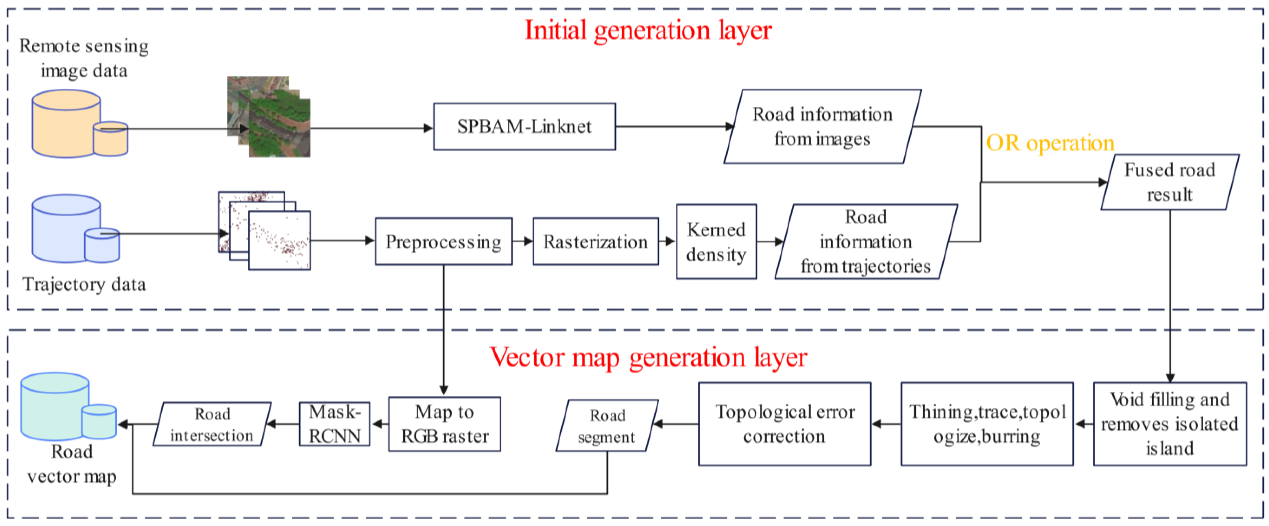
Remotesensing 15 03343 g001
Figure 2. The overall process of road extraction.
Remotesensing 15 03343 g002
Figure 3. The structure of SPBAM-Linknet.
Remotesensing 15 03343 g003
Figure 4. The left is the stop point, and the right is the drift point.
Remotesensing 15 03343 g004
Figure 5. Generating binary road images based on trajectories. (1) shows the trajectory data; (2) shows the method of selecting thresholds for sparse and dense regions of the trajectory, where (a) is the trajectory density map and (b) is the grayscale curve of the trajectory density map; (c) illu-trates the principle of linear interpolation between trajectory points, where the orange points repr-sent the actual tracking points and the green points represent the interpolated points; (3) is the pa-tition mapping result; (4) presents the results of kernel density estimation.
Remotesensing 15 03343 g005
Figure 6. The selection of the threshold value for removing isolated objects.
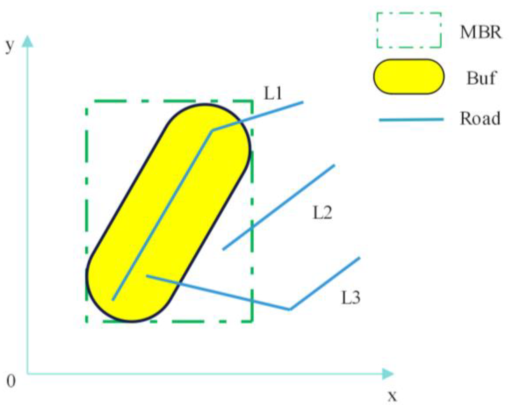
Remotesensing 15 03343 g006
Figure 7. Intersection and Connection Demonstration. The red square represents the 8-neighborhood of the triangle.
Remotesensing 15 03343 g007
Figure 8. Before (a) and after (b) the removal of “islands”.
Remotesensing 15 03343 g008
Figure 9. Topological Inconsistency Detection Methods.
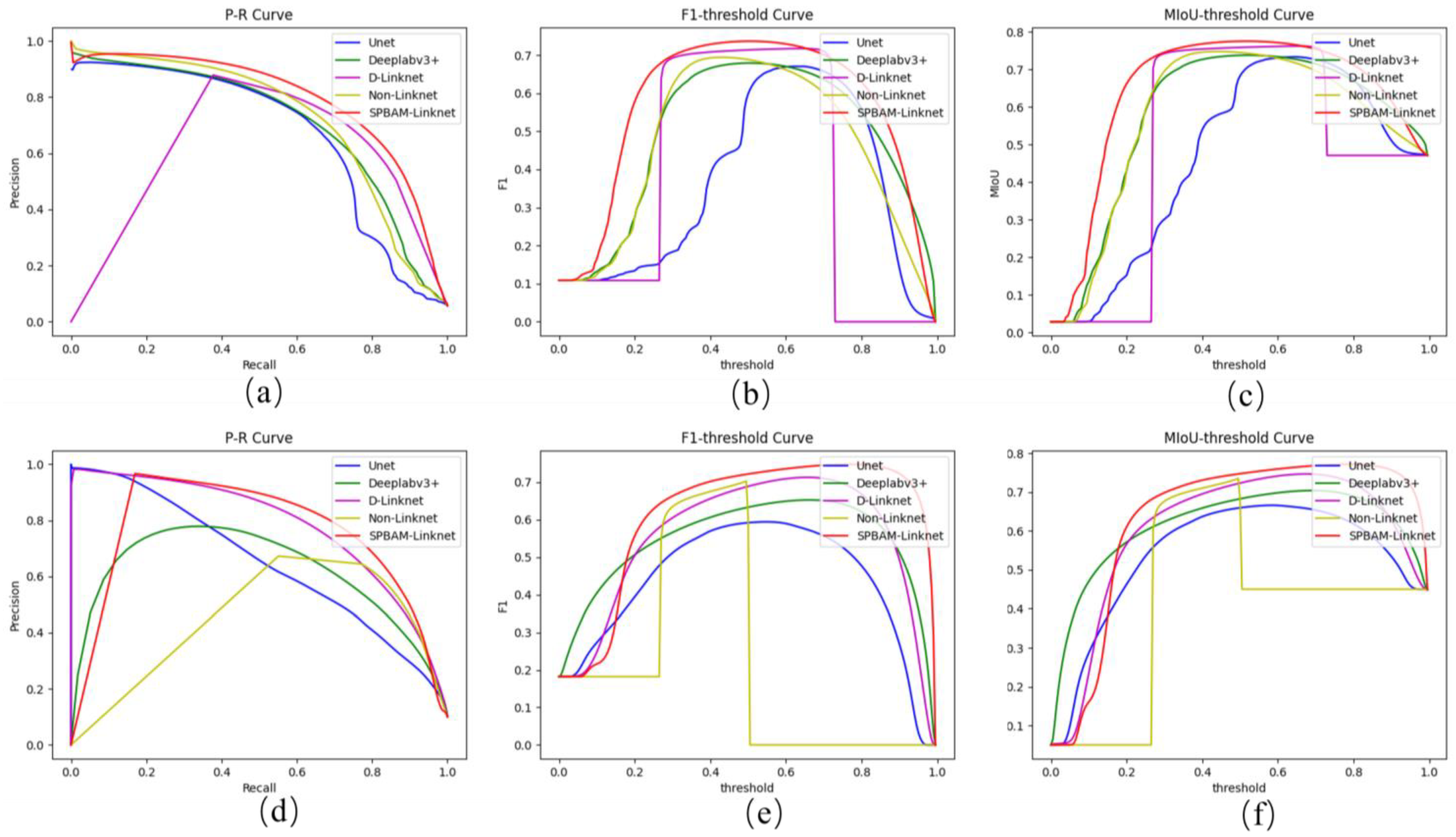
Remotesensing 15 03343 g009
Figure 10. Displays the precision–recall (P-R) curves, mean intersection-over-union (MIoU) threshold curves, and F1-score threshold curves for various neural networks on the CHN6-CUG and HB roads datasets. Panels (ac) exhibit the P-R curves, MIoU-threshold curves, and F1-threshold curves on the CHN6-CUG dataset, while panels (df) depict the corresponding curves on the HB road dataset.
Remotesensing 15 03343 g010
Figure 11. Visualization of the road extraction results of different models on the CHN6-CUG roads dataset.
Remotesensing 15 03343 g011
Figure 12. Visualization of road extraction results of different neural networks on the HB roads dataset.
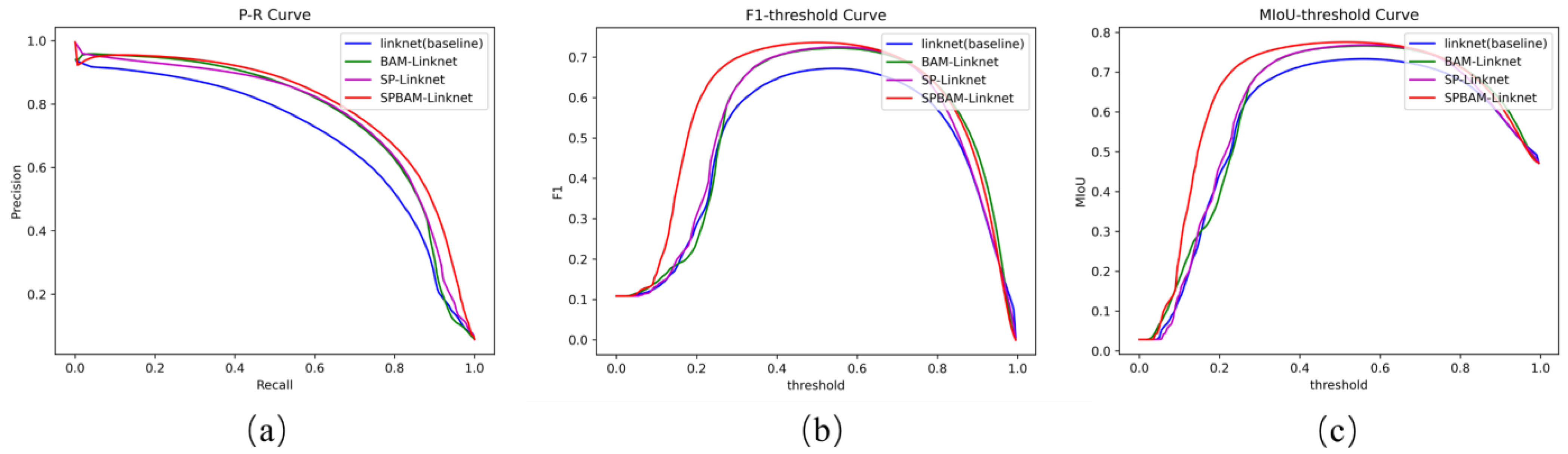
Remotesensing 15 03343 g012
Figure 13. P-R curve, F1-threshold curve, and MIoU-threshold curve of Linknet (baseline), BAM-Linknet, SP-Linknet, SPBAM-Linknet. (ac) represent the precision-recall (P-R) curve, F1-threshold curve, and mean intersection over union (MIoU) curve for LinkNet, BAM-LinkNet, SP-LinkNet, and SPBAM-LinkNet.
Remotesensing 15 03343 g013
Figure 14. Visualization of road extraction results on CHN6-CUG roads dataset with different modules adding.
Remotesensing 15 03343 g014
Figure 15. (a) is the prediction result of SPBAM-Linknet trained on CHN6-CUG roads dataset; (b) is the prediction result trained on HB roads dataset; (c) is the prediction result of CHN6-CUG roads dataset and HB roads dataset.
Remotesensing 15 03343 g015
Figure 16. Binary road images generated by trajectories with different parameters. (a) τ = 100   m , σ = 1.5   m . (b) τ = 100   m , σ = 2.25   m . (c) τ = 100   m , σ = 3   m .
Remotesensing 15 03343 g016
Figure 17. The results and treatment of road topology error detection.
Remotesensing 15 03343 g017
Figure 18. The comparison of vector results. Panel (a) illustrates the ground truth generated by OpenStreetMap (OSM) processing, while panels (bd) display the superimposed results of road segments R1, R2, and R3, respectively, with the ground truth. Areas (1,2) represent the regions where the extraction of road information using only image data failed, while areas (3,4) indicate the road information in (1,2) supplemented by trajectory data. Likewise, areas (5,6) show the regions where the extraction of road information using only trajectory data failed, and areas (7,8) depict the road information in (5,6) supplemented by image data.
Remotesensing 15 03343 g018
Figure 19. (ac) respectively represent the ground truth (GT) of vector roads, vector roads generated by RNITP, and vector roads generated by Y. Li in literature [41]. A and B are two examples where the RNITP method successfully extracted road network information, while the method reported in reference [41] failed to extract the same information.
Remotesensing 15 03343 g019
Figure 20. Failure cases of RNITP. Cases (ac) are several examples where the RNITP method failed due to reasons such as obstruction by buildings and trees, and lack of trajectory coverage.
Remotesensing 15 03343 g020
Table 1. Description of inconsistent topological relationships in vector centerlines.
Topological ErrorsDescriptionsError Type
Remotesensing 15 03343 i001This is a situation of endpoint overshooting. The scenario is that the circle exp, with the road endpoint as the center and the threshold radius r, intersects or passes through both lines str1 and str2, which intersect with each other.Overshoot
Remotesensing 15 03343 i002This is a situation of endpoint under-coverage. The scenario is that the circle exp, with the road endpoint as the center and the threshold radius r, intersects or passes through both lines str1 and str2, which are disconnected from each other.Undershoot
Remotesensing 15 03343 i003This is a situation of endpoint non-coincidence. The scenario is that the circle exp, with the road endpoint as the center and the threshold radius r, intersects all three lines str1, str2, and str3, and the lines are disconnected from one another. Alternatively, the circle exp intersects both lines str1 and str2, and the lines are disconnected from one another.Non-coincidence
Table 2. Comparison of different road extraction methods on various road datasets.
Model NameCHN6-CUG Roads DatasetHB Road Dataset
AccuracyF1MIoUAccuracyF1MIoU
Unet0.94090.59080.67870.90600.59140.6595
Deeplabv3+0.95530.67290.73010.90930.63180.6817
D-Linknet0.96730.71560.76150.92020.68740.7295
NL-Linknet0.96760.68790.74530.93560.70120.7351
SPBAM-Linknet0.96950.73690.77600.93870.72570.7514
Table 3. Results of ablation experiments on the CHN6-CUG roads dataset.
ModelBaselineBAMSPAccuracyF1MIoU
Linknet (baseline) 0.95960.66980.7307
BAM-Linknet 0.96650.72010.7638
SP-Linknet 0.96670.72200.7651
SPBAM-Linknet0.96950.73690.7760
Table 4. Statistics of road topology error results.
UndershootOvershootNon-Coincidence
The number before post-processing29071432562
The number after post-processing9812272
Corrected percentage0.96620.91480.8718
Table 5. Evaluation metrics for results.
LabelF1IoUPrecisionRecall
R10.86110.75600.86220.8599
R20.55790.38680.97060.3914
R30.88830.79910.87080.9065
Table 6. Comparison between RNITP and Y. Li et al.’s method.
MethodF1IoUPrecisionRecall
RNITP0.85180.74190.83860.8655
Y. Li et al.0.78680.64850.70270.8937
Table 7. Model complexity ranking; the serial number represents the ranking position.
ModelFLOPs of One Forward Propagation
UNet21896783462 ①
LinkNet53646196736 ②
SP-LinkNet70596986752 ③
BAM-LinkNet82715223112 ④
NL-LinkNet95878643712 ⑤
SPBAM-LinkNet99761565008 ⑥
D-LinkNet 130225799168 ⑦
Deeplabv3+169631549440 ⑧
Disclaimer/Publisher’s Note: The statements, opinions and data contained in all publications are solely those of the individual author(s) and contributor(s) and not of MDPI and/or the editor(s). MDPI and/or the editor(s) disclaim responsibility for any injury to people or property resulting from any ideas, methods, instructions or products referred to in the content.

