Article

TSVR-Net: An End-to-End Ground-Penetrating Radar Images Registration and Location Network

1
College of Electronic Science and Technology, National University of Defense Technology, Changsha 410073, China
2
Test Center, National University of Defense Technology, Xi’an 710106, China
*
Author to whom correspondence should be addressed.
Remote Sens. 2023, 15(13), 3428; https://doi.org/10.3390/rs15133428
Submission received: 31 May 2023 / Revised: 30 June 2023 / Accepted: 3 July 2023 / Published: 6 July 2023

Abstract

:
Stable and reliable autonomous localization technology is fundamental for realizing autonomous driving. Localization systems based on global positioning system (GPS), cameras, LIDAR, etc., can be affected by building occlusion or drastic changes in the environment. These effects can degrade the localization accuracy and even cause the problem of localization failure. Localizing ground-penetrating radar (LGPR) as a new type of localization can rely only on robust subsurface information for autonomous localization. LGPR is mostly a 2D-2D registration process. This paper describes the LGPR as a slice-to-volume registration (SVR) problem and proposes an end-to-end TSVR-Net-based regression localization method. Firstly, the information of different dimensions in 3D data is used to ensure the high discriminative power of the data. Then the attention module is added to the design to make the network pay attention to important information and high discriminative regions while balancing the information weights of different dimensions. Eventually, it can directly regress to predict the current data location on the map. We designed several sets of experiments to verify the method’s effectiveness by a step-by-step analysis. The superiority of the proposed method over the current state-of-the-art LGPR method is also verified on five datasets. The experimental results show that both the deep learning method and the increase in dimensional information can improve the stability of the localization system. The proposed method exhibits excellent localization accuracy and better stability, providing a new concept to realize the stable and reliable real-time localization of ground-penetrating radar images.

Graphical Abstract

1. Introduction

As the foundation of autonomous driving, autonomous localization is an important area of current research on autonomous driving technology [1]. Usually, autonomous vehicle localization requires centimetre-level localization error to ensure the vehicle’s usual driving and safe operation. The current mainstream sensors include global positioning system (GPS) [2,3], inertial motion unit (IMU) [4], cameras [5,6], and LIDAR [7,8,9,10].
Using GPS/IMU technology for localization, GPS signals may be blocked by vegetation and buildings; IMU suffers from cumulative errors. Both of these problems can degrade the localization results [1]. By iterating on trajectory matching [11] or with the help of environmental information [12], it is possible to achieve lane level navigation and localization. Camera-based localization is a current research hotspot in the field of computer vision (CV) [13,14,15], but the method is prone to mismatch under insufficient light and significant climate change. LIDAR localization can be significantly weakened or obstructed by the LIDAR beam in bad weather, such as rain or fog, and is prone to localization failure [16,17].
Ground-penetrating radar (GPR) is a new location technology that can guarantee vehicle localization accuracy in harsh environments such as a lack of road markings, insufficient light, rain, and snow. GPR is a type of radar that detects targets not visible underground or inside objects. It does not need to use information from the above-ground environment and can rely on solely robust underground information for autonomous localization.
The application of GPR systems to localization research was first used in robotics, with the main application in surveying and mapping [18,19]. The real application of GPR systems to localization started in 2013. The concept of LGPR was first introduced by Cornick and Koechling et al. at MIT Lincoln Laboratory, USA [20]. A new model of vehicle localization based on a priori maps was proposed, and LGPR systems for autonomous driving were developed. The correlation maximizing optimization technique was used to achieve registration between current images and the a priori maps. In 2020, Carnegie Mellon University identified the localization problem as a model for factor graph inference [21]. Robot localization using a learning-based sensor model in a GPS-rejected environment. This method requires the fusion of ground-penetrating radar data with odometers, and requires the ground-penetrating radar to revisit the same location. In 2022, the Chinese Academy of Sciences proposed GPR localization using DCNN assistance [22]. They constructed fingerprint maps by extracting hyperbolic features from GPR images through Fast-RCNN and accelerated the matching computation using particle swarm optimization, thus ensuring real-time localization. However, due to the uncertainty of subsurface information, the hyperbolic features were not always evident, so the abundance of subsurface targets limited the accuracy of the method subsurface. Zhang et al. focused on subsurface-rich texture stripe features, designing a point feature matching algorithm for GPR images from the perspective of edge extraction [23], and acted on texture information-rich along-track GPR data matching. However, the method detects many redundant point features on the cross-track data lacking sufficient features and could not be applied to localization tasks.
The existing LGPR is mostly a 2D-2D image registration. Due to the single structure of GPR images and few typical features, the 2D-2D registration has low discrimination power and is prone to mismatching problems. In this paper, from GPR data and scene descriptions, the essence of the LGPR problem is classified as a slice-to-volume registration (SVR) problem. The concept is derived from medical image registration and fusion and was first used in the medical field for motion correction, volume reconstruction, and image-guided interventions [24]. The traditional approach of SVR is to transform the 2D-3D registration problem into a 2D-2D-based optimal matching search problem, i.e., based on 2D-2D matching using similarity metrics, the optimal transformation is searched and solved by an optimization algorithm for registration. In recent years, with the development of deep learning technology, some new methods and models have emerged. Salehi et al. used CNN to regress the transform parameters to achieve SVR [25]. Hou et al. [26] proposed the concept of SVR-Net to use CNN to regress the transform parameters to obtain the location information of real-time slices. Deep learning methods have shown good localization and a better real-time performance in medical image registration.
In this paper, an end-to-end TSVR-Net-based regression localization method is proposed for GPR image features. By inputting a current image, the location of that image in the map data is directly predicted. Compared with the method of correlation, our method shows better stability. Furthermore, the prediction time of the method is only a few milliseconds for a single datum, showing a better real-time performance than optimization algorithms.
Our main contributions are:
We formulate the LGPR problem as an SVR problem. On this basis, we construct a twin slices-to-volume registration (TSVR) model using two data dimensions. This solves the problem of weak discriminability of the single-dimension data and improves the stability of the LGPR system.
An end-to-end TSVR-Net is designed to introduce an attention mechanism to the network to focus on important information and discriminative regions, weaken the influence of clutter interference, balance different dimensional information, and achieve the accurate and stable real-time localization.
We used the method on several datasets and validated its superiority over the state-of-the-art LGPR methods. In the rest of the sections, we first present the preparation of this work in Section 2. Then, the proposed model and methods are described in detail in Section 3. The experimental setup and parameter design are described in Section 4, and the results are analysed and discussed in Section 5. Finally, we conclude the paper in Section 6.

2. Preliminaries

2.1. Interpretation of 3D GPR Data

The GPR emits high-frequency electromagnetic waves to the ground and obtains subsurface information by analysing the reflection of electromagnetic waves received by the radar. The difference in the dielectric constant inside the detection target causes changes in the waveform and amplitude of the electromagnetic waves during propagation; therefore, it can construct GPR detection data based on this information.
The reflected signal data format received by a single-channel GPR is a one-dimensional waveform, as shown in Figure 1a, called an A-scan. The radar scanning the area of interest can obtain multiple A-scans, as shown in Figure 1b, to obtain a two-dimensional radar image, called a B-scan. The multi-channel radar scanning of the area of interest can obtain a three-dimensional image. The two-dimensional slice extracted along the along-track (x) direction is called the B-scan, containing the subsurface length–depth direction information. The two-dimensional slice extracted along the depth (t) direction is called the C-scan, containing the subsurface length–width direction information; the two-dimensional slice extracted along the cross-track (y) direction is called the D-scan, containing the subsurface width–depth direction information [27].

2.2. Principle of LGPR

Lincoln Laboratory proposed the concept of LGPR as an a priori map-based vehicle localization model. The method mainly consists of map creation and real-time localization, as shown in Figure 2. In this paper, we denote the approach proposed by MIT as the baseline method.
Among them, the subsurface environment map is created by collecting GPR data, followed by offline processing of the collected data. The processing involves slice interpolation, location label design, data pre-processing, etc. Finally, each slice of data is combined with the corresponding location label to obtain the map data with the location label. Real-time localization is a correlation calculation between a single frame of the subsurface data collected by the GPR in real-time and the previous map data using normalized correlation. Subsequently, the particle swarm optimization (PSO) algorithm [28] searches for the location with the highest correlation between the current data and the pre-stored grid data to obtain the localization results.
Later, Ort et al. [29] conducted an extended LGPR experiment under variable weather conditions and found that the real-time data in the rain and snow showed a weak correlation with the a priori map, weakening the robustness of the system navigation and localization. In this paper, we have studied and analyzed this situation. Figure 3 shows the GPR images of the same road section acquired under different weather (clear and rain), from left to right, the original, low-frequency, and high-frequency, respectively. The overall contour and shape in both images remain unchanged, but there are different degrees of variation and blurring of detail edges. By frequency domain analysis, correlations were calculated for low and high-frequency images, as shown in Table 1, and the low-frequency images showed better correlations.
The baseline is used to quantify the effect of low-frequency images on image stability. The localization results of low-frequency and raw images are plotted as line graphs, as shown in Figure 4. Multiple sets of results show that using low-frequency images could improve the stability of image registration and is more conducive to achieving robust system localization.

3. Proposed Method

In this paper, we describe the essence of a vehicle-mounted GPR localization problem as an SVR problem. Starting from the features of the GPR data, we propose a TSVR model applicable to GPR robust localization. According to the model formulation, a TSVR-Net regression network is designed based on SVR-Net, capable of end-to-end GPR localization.

3.1. TSVR Model

The localization of GPR images requires the registration of the real-time collected images with pre-collected maps. The pre-collected maps of multi-channel GPR comprises 3D volume data, and the GPR data collected in real-time is a 2D image. Therefore, the essence of the GPR localization problem is a 2D image to 3D volume data registration problem. We import the SVR model in the medical field to GPR image registration and describe the localization of GPR images as an SVR problem.
However, the number of radar channels usually limits the D-scan images acquired by multi-channel GPR in real-time. The system scans images of small size and contains few features. When this dimensional image is only used as an input to large-scale registration, mismatches are prone to occur due to the poor discrimination of single-dimensional images. Considering that GPR platform motion is a continuous process, we can achieve a more robust localization by increasing the dimensional information or the number of neighbouring slices.
We preform correlation analysis on the slice data of the three dimensions of the volume data separately, as shown in Figure 5. The smaller the red box in the image and the more concentrated the distribution, the higher the discriminative image power. By comparing the correlation surface data of the three dimensions, we found that the B-scan has stronger discriminative power in the along-track direction, and D-scan has stronger discriminative power in the cross-track direction. C-scan has more correlation peaks in volume with weaker overall discriminative power. To address the characteristics of the three dimensions of the GPR data, we select B-scan and D-scan data as the registration images and use the increase in data dimensions to improve the stability of the system localization. We propose a TSVR model applicable to localizing GPR. The model can be abstracted into the following mathematical representation:
T = argmax T M ( S , V ; T )
where S = S cross , S along denotes the set of 2D slices obtained during real-time localization, where S cross denotes the slice in the cross-track direction that corresponds to the D-scan image, and S along denotes the slice in the along-track direction that corresponds to the B-scan image. They are used to form the data form of the T-slices, as shown in Figure 6. V denotes the pre-stored 3D data map, and M denotes the image similarity metric.

3.2. Attention Mechanism

GPR images have obvious media layering and hyperbolic structural features, as shown in Figure 7. These two regions can provide more features for image registration. Therefore, paying attention to the media layering and hyperbolic feature regions in GPR image registration is an effective strategy to improve registration accuracy.
As an effective way to control feature weights, the attention mechanism is widely used in CV [30] such as image classification [31,32], target detection [33], and medical image processing [34]. We add the attention mechanism to GPR image registration by combining spatial and channel attention to select image regions and features with high discriminative power.

3.2.1. Channel Attention Mechanism: ECA-Net

ECA-Net [35] is a local cross-channel interaction strategy that does not utilize dimensionality reduction. It can adaptively select the size of a one-dimensional convolution kernel. The network module is shown in Figure 8. It can obtain significant performance gains without increasing model complexity. Firstly, differing from attention mechanisms such as SE-Net [31], ECA-Net avoids the effect of dimensional reduction on the channel attention learning effect. Secondly, ECA-Net implements a local cross-channel interaction strategy using 1 × 1 convolution to achieve adaptive adjustment of the convolution kernel size k, calculated by:
k = ψ ( C ) = log 2 ( C ) γ + b γ odd
where C is the input channel dimension, γ = 2 , b = 1 , and | t | odd denotes the nearest odd.

3.2.2. Spatial Attention Mechanism

Spatial attention is a module that enhances feature representation of critical regions of the image. The spatial attention module first reduces the dimension of the channel to obtain the maximum and mean pooling results. Second, the two pooling results are stitched together in the channel dimension, and the convolutional layers fuse the features. Finally, spatial feature weight descriptors are generated by the sigmoid operation. The descriptors are superimposed onto the original image to enhance the feature representation of critical regions in the image.

3.3. Twin Slices-to-Volume Registration Net

Based on the formulation of the TSVR model, we propose a TSVR-Net based model on the SVR-Net study [26]. This model can realize the end-to-end location parameter regression prediction (due to the limitation of network generalization capability, it is more challenging to achieve end-to-end image registration. However, since the GPR localization problem is based on a priori map registration, each road is trained separately to require less generalization capability to achieve the end-to-end network prediction), with the network architecture is shown in Figure 8, mathematically represented by:
T ^ i = ψ ω i , θ
where θ denotes the network parameters and ω i V denotes a series of slice sets obtained from the volume data V.
Through the analysis of different weather GPR images in Section 2.2, we demonstrate that low-frequency information enables more robust localization. Therefore, a mean pooling layer is added to the network to achieve low-pass filtering [36], leading to more robust registration.
The SVR-Net regression network only uses information from a single dimension and will show lower discriminability in another dimension, affecting the accuracy of the registration. TSVR-Net fully utilizes the volume data information of GPR images as well as B-scan and D-scan two-dimensional information. It can improve the amount of information while ensuring the image set has high discriminative power. However, since the B-scan and D-scan correspond to different physical resolutions and polarization methods when the multi-channel radar performs data acquisition, using the same parameter weights for feature extraction will deteriorate the extraction effect. Therefore, we do not use parameter sharing for image feature extraction but train the two dimensions separately and perform feature fusion on the extracted underlying features to obtain the fused feature F 1 .
F 1 = f concat f 1 S cross , f 2 S along
where, f 1 ( ) and f 2 ( ) denote the feature extraction for D-scan and B-scan images, respectively. f c o n c a t ( ) denotes feature concatenation performed for channel dimensions in this network.
Due to the unknown nature of subsurface information, the image information distribution of different road regions is different. In order to make full use of the rich regions of image information, we start from two perspectives. Firstly, we combine channel attention and spatial attention when extracting the image features [32], paying attention to the features in the regions with higher image discrimination. Secondly, we add the channel attention mechanism to control the weights of each dimension in the regression when fusing the features of different dimensions to obtain the new fused features F. Subsequently, we input F into the network for training.
F = ϕ f concat φ 1 f 1 S cross , φ 2 f 2 S along
where φ 1 ( ) and φ 2 ( ) denote the channel and spatial attention to the D-scan and B-scan image features, respectively, and ϕ ( ) denotes the channel attention mechanism. The spatial attention finds the important parts of the image for processing. First, the channel itself is downscaled to obtain the results of maximum pooling and average pooling. Then the two pooling results are concatenated in the channel dimension and fed into a one-dimensional convolution. ECA-Net is used for channel attention.
Finally, the feature vectors extracted from all channels of the convolutional layer are connected and integrated using a fully-connected layer. To reduce the possibility of overfitting, the network design adds a dropout layer between the fully connected layers, and finally, each output node corresponds to a localization parameter T ^ i .

4. Experiment and Parameter Design

4.1. Data Collection

In this section, we evaluate the network’s performance through experimental validation and compare it with the baseline. To perform a comprehensive evaluation of the proposed method, we performed multiple sets of experimental data acquisition in different outdoor scenarios, containing various conditions such as different times and weather. The system platform used for data acquisition is shown in Figure 9, mainly including 3D-Radar, distance measuring instrument (DMI), a vehicle-mounted platform, a real-time kinematic (RTK) and a high-performance computer. The detailed parameter settings of the system are shown in Table 2. The experimental site was selected at the Yuntang campus of Changsha University of Technology, and the collected data are shown in Figure 10.
First, we study high-precision registration and localization. To reduce the impact of multi-sensor errors, data collection is strictly collected according to the preset track. The starting point is strictly aligned during data recording and travels in a straight line according to the preset track. The DMI external trigger is used to operate the GPR system, and the DMI data provides the location truth. At the same time, we analyse the effect of the proposed method for navigation and localization with the data truth provided by RTK.

4.2. Data Preparation

Maps and real-time slices are prepared based on the collected data and used in the baseline and proposed methods. The GPR data were preprocessed using the 3D-Radar software 3dr-Examiner for background removal.
The baseline method can extract a single D-scan image from the 3D data directly for registration. For the proposed method, the data production is borrowed from the triplanar structure of GPR target detection [37]. The first step is to extract the three-dimensional mask window from the volume data according to the radar system to determine the window size set to x , y , z . The width is defined by the number of channels in the multi-channel GPR system. The length is consistent with the number of channels to ensure the integrity of the information depth towards taking the full depth of the acquisition. Both x and y are 20 pixels and the z-axis is represents the depth-wise sampling points of the corresponding data.
The window is panned across the along-track and cross-track directions to obtain multiple 3D masks, as shown in Figure 6. The last slice of the D-scan and corresponding B-scan of the 10th channel in each mask window is taken as the slicing group for network training and testing.

4.3. Methods and Parameter Setup

To verify the rationality of our proposed method, we compare it to the other five methods in Table 3. Among them, the baseline method is the most state-of-the-art algorithm in GPR image localization, and the SVR-A, SVR-C, SVR-TC, and SVR-FC methods are the step-by-step verification of the rationality of our proposed method. SVR-A and SVR-C are used to demonstrate the feasibility of predicting location parameters using SVR-Net regression. SVR-TC and SVR-FC verify the improvement in system localization performance by introducing twin slice information. SVR-TC trains two-dimensional images as a two-channel (TC) input network of one tensor. SVR-FC inputs images of two dimensions into two networks, respectively, and performs feature concatenation (FC) after the second convolution. Multiple sets of ablation experiments are conducted to analyse the localization effect of the proposed TSVR-Net.
The baseline experimental platform uses MATLAB 2019b and a 3.2 GHz AMD CPU. Among them, the PSO method is a 3DOF search. The main parameters include a population size of 80 and an iteration number of 100. All experiments for the deep learning method were trained on a computer with an NVIDIA RTX 3060 GPU, and the data were tested using the CPU.

5. Results and Discussion

In this section, we identify and analyse the superiority of the attention mechanism in terms of network performance through visualization. Furthermore, we compare the localization effect of the proposed algorithm against the five methods mentioned in Section 4.3.

5.1. Network Training Visualization

Three networks that can extract individual D-scan feature maps, TSVR, SVR-C, and SVR-FC, are selected to visualize the effect of feature map extraction. The feature images before extracting the conv3 of these three networks are shown in Figure 11. We find that the SVR-C network, which does not incorporate the attention mechanism, learns features with low differentiation, and the features are fuzzy and similar to each other. The SVR-FC network utilizes shallower and less stable information in the subsurface, not conducive to achieving robust registration and localization. The TSVR extracts features from a wider distribution area, including the upper-medium stratification information and the deeper robust information. TSVR gives different weights to different spatial regions and feature maps, showing a more favourable effect on feature extraction for registration and localization.

5.2. Quantitative Analysis

We have collected data on three common types of pavements: masonry, asphalt, and cement, including different conditions at different times of the day and in different weather.
Table 4 records the type of data collected, and information about the road section, weather, lane, and road length. The amount of information is calculated for the collected road sections, and the data is quantified using grey information entropy, expressed as:
H = i p i log 2 p i
where p i represents the number of pixels whose grey value is i, and the higher the information entropy is, the more information it contains. We quantify the B-scan collected data for each road section to obtain the information volume of each road section, as shown in Table 5.
We classified the measured data to produce five different datasets, subsequently quantifying the proposed method on these five datasets. The calculation of the localization error is performed using the l 2 parametric number, denoted as error = T ^ i T i 2 . The statistical error distribution is also plotted as a boxplot, as shown in Figure 12, for the statistical error distribution of the localization accuracy on the five datasets under the six methods. The B-scan images of each dataset are shown in Figure 13.

5.2.1. The Same Weather of Asphalt Pavement

This dataset contains GPR data collected on the same asphalt road section during clear weather. The B-scan image shows that the underground media in this area is clearly layered and has obvious underground targets. From the information entropy, this dataset contains a high amount of information. The data includes left, centre, and right images [38]. The complete images obtained by concatenating the left and right are used as the map data for this dataset, while the centre is used as real-time images for testing, as shown in Figure 14.
As shown in Table 6 and Figure 12a, the proposed method outperforms the baseline method in terms of localization. The SVR-based deep learning method has less long-range dispersion than the baseline, indicating that the deep learning-based localization method is more robust.
The localization effect of the SVR-C method is slightly better than the SVR-A method on this dataset. By adding dimensional information, the SVR-TC and SVR-FC methods have similar results in terms of localization accuracy as the SVR-A and SVR-C methods only using a single dimension; however, the stability of the localization is higher, indicating that adding dimensional information can improve the stability of localization. Among them, the TSVR method, which utilizes multi-dimensional information and attention mechanisms, performs best, indicating that increasing the dimensional information effectively improves the localization accuracy. However, attention needs to be paid to the valid information of each dimension.

5.2.2. The Same Weather of Masonry Pavement

Dataset B comprises GPR data from multiple trips to the masonry section collected in clear weather at different times. There are abundant subsurface targets under the masonry sections, but there are undulations in the road surface and significant clutter interference. The data form is the same as dataset A.
As shown in Table 7 and Figure 12b, the localization effect on the dataset of the masonry road section was degraded compared to the asphalt road section. This is likely due to the large clutter interference on the road section, which deteriorates the localization effect. However, our proposed method still outperforms the baseline method. The existence of clutter interference seriously affects the stability of single-slice registration. Currently, the SVR-TC, SVR-FC, and TSVR methods with increased dimensional information all show higher stability than the single-slice method. SVR-TC and SVR-FC have better localization accuracy than SVR-C but still have a gap with SVR-A. In comparison, the TSVR method still shows the best localization accuracy and better stability.

5.2.3. The Same Weather of Cement Pavement

Dataset C contains GPR data collected from multiple cement road sections during clear weather at different times. There are no obvious underground targets or media stratification in this section. From the B-scan image, it is challenging to observe obvious underground targets and media stratification, and from the information entropy, the road section contains less information.
As shown in Table 8 and Figure 12c, the performance of the baseline method significantly decreases on road sections with no obvious targets and less information. At the same time, most of the SVR methods have a lower decline with a substantially better localization performance than the baseline method. This proves that the SVR method is still effective in locating GPR data with limited information.
By comparing the two methods, SVR-A and SVR-C, we find that the SVR-A method is significantly worse than the SVR-C method for this dataset. This difference may be caused by different polarization methods and subsurface feature distribution, indicating the poor discrimination of B-scan images for sections with less information. The three methods of adding dimensional information showed significant advantages at this time. The localization error of the TSVR method is only 0.2528 m, much lower than the SVR-A method at 0.8275 m. This indicates that image discrimination is low when the amount of information is low, and it is very effective to increase the amount of information by introducing multiple slices to improve the discrimination of image matching.

5.2.4. Different Weather of Asphalt Pavement

Dataset D comprises GPR data of the same asphalt pavement collected in different weather conditions (clear and rain days). The underground features in this area are consistent with dataset A. However, the subsurface water content changes with the weather, and there are different degrees of variation and blurring in the images on clear and rain days.
As shown in Table 9 and Figure 12d, compared with dataset A, both the baseline and SVR methods have more discrete values, and the localization performance is degraded. However, the TSVR method still outperforms the baseline method and has higher localization accuracy and stability.
In this dataset, we find that the localization accuracy of both the SVR-TC and SVR-FC methods is significantly worse than the method using only a single slice. Due to the rich feature information in this section, the single-dimensional image already has high discriminative power. Although increasing the dimensionality can increase the amount of information, utilizing it without screening can weaken the discriminatory power of the image and deteriorate the localization effect. The TSVR method, which also adds dimensional information, still shows the best localization effect among all the methods, indicating that introducing an attention mechanism when utilizing multi-dimensional information is very effective.

5.2.5. Different Weather of Masonry Pavement

Dataset E contains GPR data of the same masonry pavement collected in different weather conditions (clear and rain days). The subsurface characteristics of this area are consistent with dataset B. However, because the drainage performance of the masonry section is weaker than the asphalt pavement, the difference in images between clear and rain days is more pronounced.
The dielectric constant affects the GPR data, which are more pronounced in the masonry pavement than in the asphalt pavement. Therefore, the localization performance is degraded under this dataset, as shown in Table 10.
Although the localization performance of all the methods degrades, the baseline degradation is more evident than that of the SVR method, and the localization effect of the proposed method is still significantly better than that of the baseline. This demonstrates the effectiveness of the proposed method in LGPR problems and its robustness to weather variations.
Further, we find their effects are similar under this dataset by comparing the four methods of SVR-A, SVR-C, SVR-FC, and SVR-TC. However, the TSVR method still shows the optimal effect, indicating that the TSVR method is most suitable for GPR localization problems in various situations with high stability.
Table 11 shows the average run time for a single sample of each method in the five datasets. To visually represent the localization effect of the TSVR method, we plotted the localization track of the TSVR method in the World Geodetic System 1984 (WGS-84) coordinate system on a section of road about 250 m long, as shown in Figure 15. Finally, we summarized the analysis of the results as follows.
The rich subsurface information is beneficial to the matching localization of GPR images. The proposed and baseline methods both show better localization results in the subsurface target-rich and media-stratified road sections corresponding to datasets A and B.
Weather changes can deteriorate the stability of system localization. Datasets D and E both have worse localization error than datasets A and B for both the baseline and deep learning methods.
The use of deep learning methods can ensure higher stability of system localization. Comparing the baseline and SVR-C methods, SVR-C outperforms the baseline method in terms of the mean and variance of errors.
Increasing the dimensional information of GPR images is beneficial to improve the stability of the localization system. Comparing SVR-TC, SVR-FC, and TSVR with SVR-A and SVR-C, the former three with increased dimensional information showed significant advantages on a larger number of datasets.
Deep learning methods have higher real-time performance and nearly 60 times faster location prediction speed than the baseline method, which could be better applied to real-time localization.
The TSVR method combines multi-dimensional and attention mechanisms to show optimal localization accuracy as well as better stability on all five datasets, significantly improving the accuracy, stability and real-time performance of GPR image localization.

6. Conclusions

GPR localization is a new mode based on map localization, utilizing underground robust features to achieve reliable autonomous localization in environments such as GPS rejection and harsh weather. In this paper, we described GPR localization as an SVR model and proposed an end-to-end regression localization network. At the same time, in response to the low information content of GPR images, we used mutually perpendicular data slices to increase the information content of GPR images, thus proposing the TSVR model. The increase in information volume not only brings more robust features, but also adds new interference. Therefore, we have added an attention mechanism module in the network design to balance the information weights of two dimensions in the network, focusing on robust feature regions and ensuring that GPR images have high discrimination.
We constructed five datasets with different road sections and weather conditions by actual acquisition and verified the effectiveness of the proposed method step by step on the five datasets. The experimental results show that the proposed method can improve the discrimination of GPR images and achieve more robust matching localization. Compared with the baseline, our method significantly improves the accuracy and stability of GPR system localization with stronger real-time performance. Although the proposed method shows some advantages in accuracy, stability, and real-time acquisition, the amount of map storage data for network training increased compared to the original data. Based on this work, we hope to gradually realize the compression of the training storage data for the realistic deployment of this system.

Author Contributions

Conceptualization, B.B. and L.S.; methodology, B.B.; validation, B.B. and L.S.; formal analysis, B.B.; investigation, P.Z.; resources, X.H., Q.X. and T.J.; writing—original draft preparation, B.B. All authors have read and agreed to the published version of the manuscript.

Funding

This research received no external funding.

Data Availability Statement

Data sharing not applicable.

Acknowledgments

The authors would like to thank the State Key Laboratory, Changsha University of Science and Technology, Changsha, China for providing equipment support.

Conflicts of Interest

The authors declare no conflict of interest.

References

  1. Kuutti, S.; Fallah, S.; Katsaros, K.; Dianati, M.; Mccullough, F.; Mouzakitis, A. A survey of the state-of-the-art localization techniques and their potentials for autonomous vehicle applications. IEEE Internet Things J. 2018, 5, 829–846. [Google Scholar] [CrossRef]
  2. Djuknic, G.M.; Richton, R.E. Geolocation and assisted GPS. Computer 2001, 34, 123–125. [Google Scholar] [CrossRef] [Green Version]
  3. Tan, H.S.; Huang, J. DGPS-based vehicle-to-vehicle cooperative collision warning: Engineering feasibility viewpoints. IEEE Trans. Intell. Transp. Syst. 2006, 7, 415–428. [Google Scholar] [CrossRef]
  4. Zhang, F.; Stähle, H.; Chen, G.; Simon, C.C.C.; Buckl, C.; Knoll, A. A sensor fusion approach for localization with cumulative error elimination. In Proceedings of the 2012 IEEE International Conference on Multisensor Fusion and Integration for Intelligent Systems (MFI), Hamburg, Germany, 13–15 September 2012; IEEE: Piscataway Township, NJ, USA, 2012; pp. 1–6. [Google Scholar]
  5. Li, C.; Dai, B.; Wu, T. Vision-based precision vehicle localization in urban environments. In Proceedings of the 2013 Chinese Automation Congress, Changsha, China, 7–8 November 2013; IEEE: Piscataway Township, NJ, USA, 2013; pp. 599–604. [Google Scholar]
  6. Parra, I.; Sotelo, M.A.; Llorca, D.F.; Ocaña, M. Robust visual odometry for vehicle localization in urban environments. Robotica 2010, 28, 441–452. [Google Scholar] [CrossRef] [Green Version]
  7. Hata, A.Y.; Wolf, D.F. Feature detection for vehicle localization in urban environments using a multilayer LIDAR. IEEE Trans. Intell. Transp. Syst. 2015, 17, 420–429. [Google Scholar] [CrossRef]
  8. Wolcott, R.W.; Eustice, R.M. Fast LIDAR localization using multiresolution Gaussian mixture maps. In Proceedings of the 2015 IEEE International Conference on Robotics and Automation (ICRA), Seattle, WA, USA, 26–30 May 2015; IEEE: Piscataway Township, NJ, USA, 2015; pp. 2814–2821. [Google Scholar]
  9. Tao, Q.; Hu, Z.; Zhou, Z.; Xiao, H.; Zhang, J. SeqPolar: Sequence Matching of Polarized LiDAR Map with HMM for Intelligent Vehicle Localization. IEEE Trans. Veh. Technol. 2022, 71, 7071–7083. [Google Scholar] [CrossRef]
  10. Chen, G.; Lu, F.; Li, Z.; Liu, Y.; Dong, J.; Zhao, J.; Yu, J.; Knoll, A. Pole-curb fusion based robust and efficient autonomous vehicle localization system with branch-and-bound global optimization and local grid map method. IEEE Trans. Veh. Technol. 2021, 70, 11283–11294. [Google Scholar] [CrossRef]
  11. Yan, Z.; Zhang, C.; Yang, Y.; Liang, J. A novel in-motion alignment method based on trajectory matching for autonomous vehicles. IEEE Trans. Veh. Technol. 2021, 70, 2231–2238. [Google Scholar] [CrossRef]
  12. Gu, Y.; Hsu, L.T.; Kamijo, S. GNSS/onboard inertial sensor integration with the aid of 3-D building map for lane-level vehicle self-localization in urban canyon. IEEE Trans. Veh. Technol. 2015, 65, 4274–4287. [Google Scholar] [CrossRef]
  13. Xiong, Z.; Cai, Z.; Han, Q.; Alrawais, A.; Li, W. ADGAN: Protect your location privacy in camera data of auto-driving vehicles. IEEE Trans. Ind. Inform. 2020, 17, 6200–6210. [Google Scholar] [CrossRef]
  14. Beklemishev, N. Direct Solution for Estimating the Location of the Central Projection Camera by Four Control Points. Math. Model. Comput. Simul. 2021, 13, 512–521. [Google Scholar] [CrossRef]
  15. Dong, J.; Ren, X.; Han, S.; Luo, S. UAV Vision Aided INS/Odometer Integration for Land Vehicle Autonomous Navigation. IEEE Trans. Veh. Technol. 2022, 71, 4825–4840. [Google Scholar] [CrossRef]
  16. Levinson, J.; Montemerlo, M.; Thrun, S. Map-based precision vehicle localization in urban environments. In Robotics: Science and Systems; Citeseer: State College, PA, USA, 2007; Volume 4, p. 1. [Google Scholar]
  17. Lowry, S.; Sünderhauf, N.; Newman, P.; Leonard, J.J.; Cox, D.; Corke, P.; Milford, M.J. Visual place recognition: A survey. IEEE Trans. Robot. 2015, 32, 1–19. [Google Scholar] [CrossRef] [Green Version]
  18. Williams, R.M.; Ray, L.E.; Lever, J. An autonomous robotic platform for ground penetrating radar surveys. In Proceedings of the 2012 IEEE International Geoscience and Remote Sensing Symposium, Munich, Germany, 22–27 July 2012; IEEE: Piscataway Township, NJ, USA, 2012; pp. 3174–3177. [Google Scholar]
  19. Lever, J.H.; Delaney, A.J.; Ray, L.E.; Trautmann, E.; Barna, L.A.; Burzynski, A.M. Autonomous gpr surveys using the polar rover yeti. J. Field Robot. 2013, 30, 194–215. [Google Scholar] [CrossRef]
  20. Cornick, M.; Koechling, J.; Stanley, B.; Zhang, B. Localizing ground penetrating radar: A step toward robust autonomous ground vehicle localization. J. Field Robot. 2016, 33, 82–102. [Google Scholar] [CrossRef]
  21. Baikovitz, A.; Sodhi, P.; Dille, M.; Kaess, M. Ground encoding: Learned factor graph-based models for localizing ground penetrating radar. In Proceedings of the 2021 IEEE/RSJ International Conference on Intelligent Robots and Systems (IROS), Prague, Czech Republic, 27 September–1 October 2021; IEEE: Piscataway Township, NJ, USA, 2021; pp. 5476–5483. [Google Scholar]
  22. NI, Z.; YE, S.; SHI, C.; PAN, J.; ZHENG, Z.; FANG, G. A Deep Learning Assisted Ground Penetrating Radar Localization Method. J. Electron. Inf. Technol. 2022, 44, 1265–1273. [Google Scholar]
  23. Zhang, P.; Shen, L.; Huang, X.; Xin, Q. A new registration method with improved phase congruency for application to GPR images. Remote Sens. Lett. 2022, 13, 726–737. [Google Scholar] [CrossRef]
  24. Ferrante, E.; Paragios, N. Slice-to-volume medical image registration: A survey. Med. Image Anal. 2017, 39, 101–123. [Google Scholar] [CrossRef] [PubMed] [Green Version]
  25. Salehi, S.S.M.; Khan, S.; Erdogmus, D.; Gholipour, A. Real-time deep pose estimation with geodesic loss for image-to-template rigid registration. IEEE Trans. Med. Imaging 2018, 38, 470–481. [Google Scholar] [CrossRef]
  26. Hou, B.; Alansary, A.; McDonagh, S.; Davidson, A.; Rutherford, M.; Hajnal, J.V.; Rueckert, D.; Glocker, B.; Kainz, B. Predicting slice-to-volume transformation in presence of arbitrary subject motion. In Proceedings of the International Conference on Medical Image Computing and Computer-Assisted Intervention, Quebec City, QC, Canada, 11–13 September 2017; Springer: Berlin/Heidelberg, Germany, 2017; pp. 296–304. [Google Scholar]
  27. Kim, N.; Kim, S.; An, Y.K.; Lee, J.J. A novel 3D GPR image arrangement for deep learning-based underground object classification. Int. J. Pavement Eng. 2021, 22, 740–751. [Google Scholar] [CrossRef]
  28. Kennedy, J.; Eberhart, R. Particle swarm optimization. In Proceedings of the ICNN’95-International Conference on Neural Networks, Perth, Australia, 27 November–1 December 1995; IEEE: Piscataway Township, NJ, USA, 1995; Volume 4, pp. 1942–1948. [Google Scholar]
  29. Ort, T.; Gilitschenski, I.; Rus, D. Autonomous navigation in inclement weather based on a localizing ground penetrating radar. IEEE Robot. Autom. Lett. 2020, 5, 3267–3274. [Google Scholar] [CrossRef]
  30. Guo, M.H.; Xu, T.X.; Liu, J.J.; Liu, Z.N.; Jiang, P.T.; Mu, T.J.; Zhang, S.H.; Martin, R.R.; Cheng, M.M.; Hu, S.M. Attention mechanisms in computer vision: A survey. Comput. Vis. Media 2022, 8, 331–368. [Google Scholar] [CrossRef]
  31. Hu, J.; Shen, L.; Albanie, S.; Sun, G.; Wu, E. Squeeze-and-Excitation Networks. IEEE Trans. Pattern Anal. Mach. Intell. 2019, 7132–7141. [Google Scholar]
  32. Woo, S.; Park, J.; Lee, J.Y.; Kweon, I.S. Cbam: Convolutional block attention module. In Proceedings of the European Conference on Computer Vision (ECCV), Munich, Germany, 8–14 September 2018; pp. 3–19. [Google Scholar]
  33. Dai, J.; Qi, H.; Xiong, Y.; Li, Y.; Zhang, G.; Hu, H.; Wei, Y. Deformable convolutional networks. In Proceedings of the IEEE International Conference on Computer Vision, Venice, Italy, 22–29 October 2017; pp. 764–773. [Google Scholar]
  34. Guan, Q.; Huang, Y.; Zhong, Z.; Zheng, Z.; Zheng, L.; Yang, Y. Thorax disease classification with attention guided convolutional neural network. Pattern Recognit. Lett. 2020, 131, 38–45. [Google Scholar] [CrossRef]
  35. Wang, Q.; Wu, B.; Zhu, P.; Li, P.; Zuo, W.; Hu, Q. ECA-Net: Efficient Channel Attention for Deep Convolutional Neural Networks. In Proceedings of the 2020 IEEE/CVF Conference on Computer Vision and Pattern Recognition (CVPR), Seattle, WA, USA, 13–19 June 2020. [Google Scholar]
  36. Boroumand, M.; Chen, M.; Fridrich, J. Deep residual network for steganalysis of digital images. IEEE Trans. Inf. Forensics Secur. 2018, 14, 1181–1193. [Google Scholar] [CrossRef]
  37. Kim, N.; Kim, S.; An, Y.K.; Lee, J.J. Triplanar imaging of 3-D GPR data for deep-learning-based underground object detection. IEEE J. Sel. Top. Appl. Earth Obs. Remote Sens. 2019, 12, 4446–4456. [Google Scholar] [CrossRef]
  38. Ort, T.; Gilitschenski, I.; Rus, D. GROUNDED: The Localizing Ground Penetrating Radar Evaluation Dataset. In Proceedings of the Robotics: Science and Systems 2021, Online, 12–16 July 2021; Volume 2. [Google Scholar]
Figure 1. GPR data formats and images. The top image represents the data format of the GPR reflections, where the x-axis represents the vehicle travel direction (along-track), the y-axis represents the radar channel dimension direction (cross-track), and the t-axis represents the time (depth) dimension of the radar’s downward data acquisition. The image at the bottom is the waveform or image representation of the data collected by GPR in each dimension. From left to right are the A-scan, B-scan, C-scan, D-scan, and 3D data.
Remotesensing 15 03428 g001
Figure 2. LGPR localization process. The process is mainly divided into map creation in the solid box and real-time localization in the dashed box. Firstly, the pre-collected data and location labels are interpolated to the grid to obtain the map data with GPR data and location labels. Then, the current scanned image is registered to the grid map, and the corresponding localization label of the image marked by the red box is obtained through registration.
Remotesensing 15 03428 g002
Figure 3. GPR image correlation in clear and rainy weather. The first and second rows show the analysis of the GPR images obtained from scanning the same road section on clear and rainy days, respectively. The left side is the raw image scanned, the middle is the low-frequency image, and the right is the high-frequency image.
Remotesensing 15 03428 g003
Figure 4. Comparison of baseline localization errors between low-frequency and raw images. The line graph plots the error obtained by comparing the registration localization with the actual localization for 30 sets of data using the baseline. The blue line in the figure indicates the localization error of the low-frequency image registration, and the red line indicates the localization error of the raw image registration.
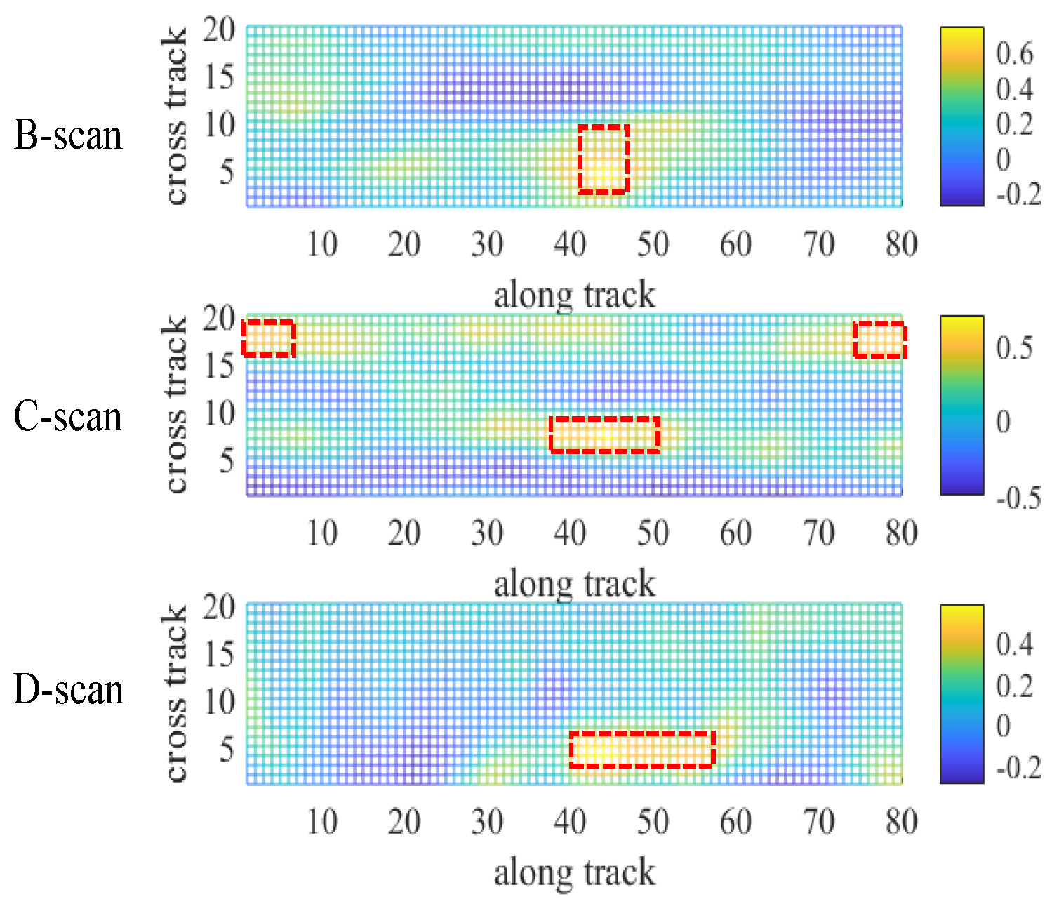
Remotesensing 15 03428 g004
Figure 5. Correlation surface analysis of the sliced data in different dimensions. From top to bottom are the correlation surface results for the B-scan, C-scan, and D-scan on the volume at the location (45, 4, 0) of the volume data, respectively. The bright yellow colour in the image indicates a correlation of 1, and the dark blue colour indicates a correlation of −1, where the red box area is the correlation peak area.
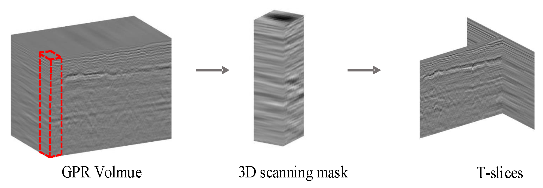
Remotesensing 15 03428 g005
Figure 6. T-slices production process.
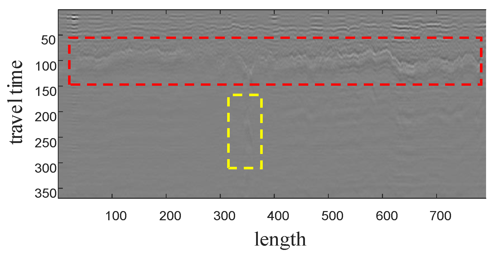
Remotesensing 15 03428 g006
Figure 7. Typical GPR image. The red box region in the image has a clear black-white layering, demonstrating the layered characteristics of the GPR image, caused by the different dielectric constants of different geological layers. The yellow box region in the image demonstrates the hyperbolic feature of the subsurface target reacting to the image.
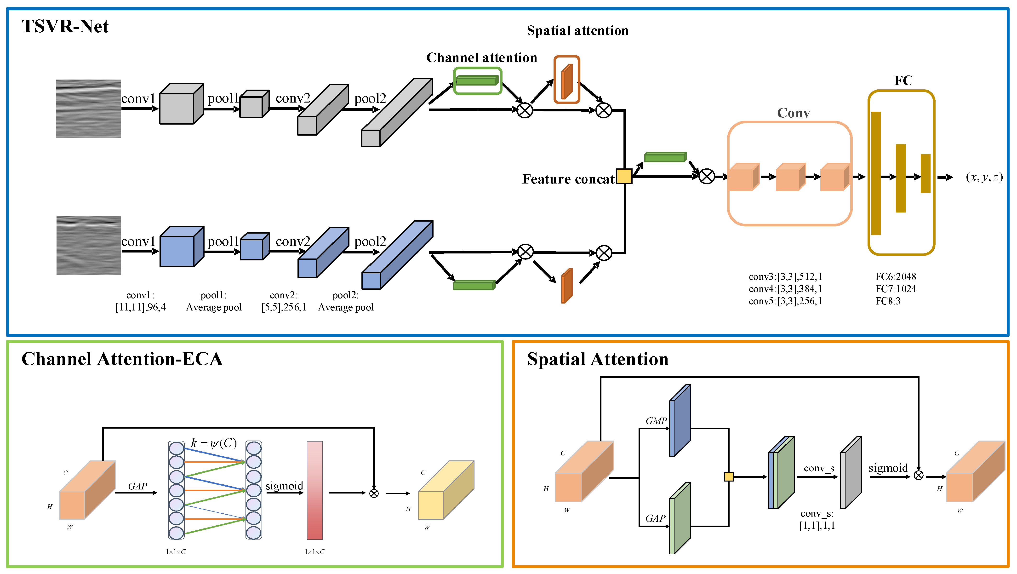
Remotesensing 15 03428 g007
Figure 8. The architecture of our network and attention modules. The blue box shows the architecture of our network. The green box is the channel attention module (using ECA). The orange box is the spatial attention module. The convolutional layer configuration is denoted as: kernel size, number of channels, and stride. GAP denotes global average pooling. GMP denotes global max pooling. The symbol indicates matrix multiplication. Feature concatenation is fusion of all the channel dimensions.
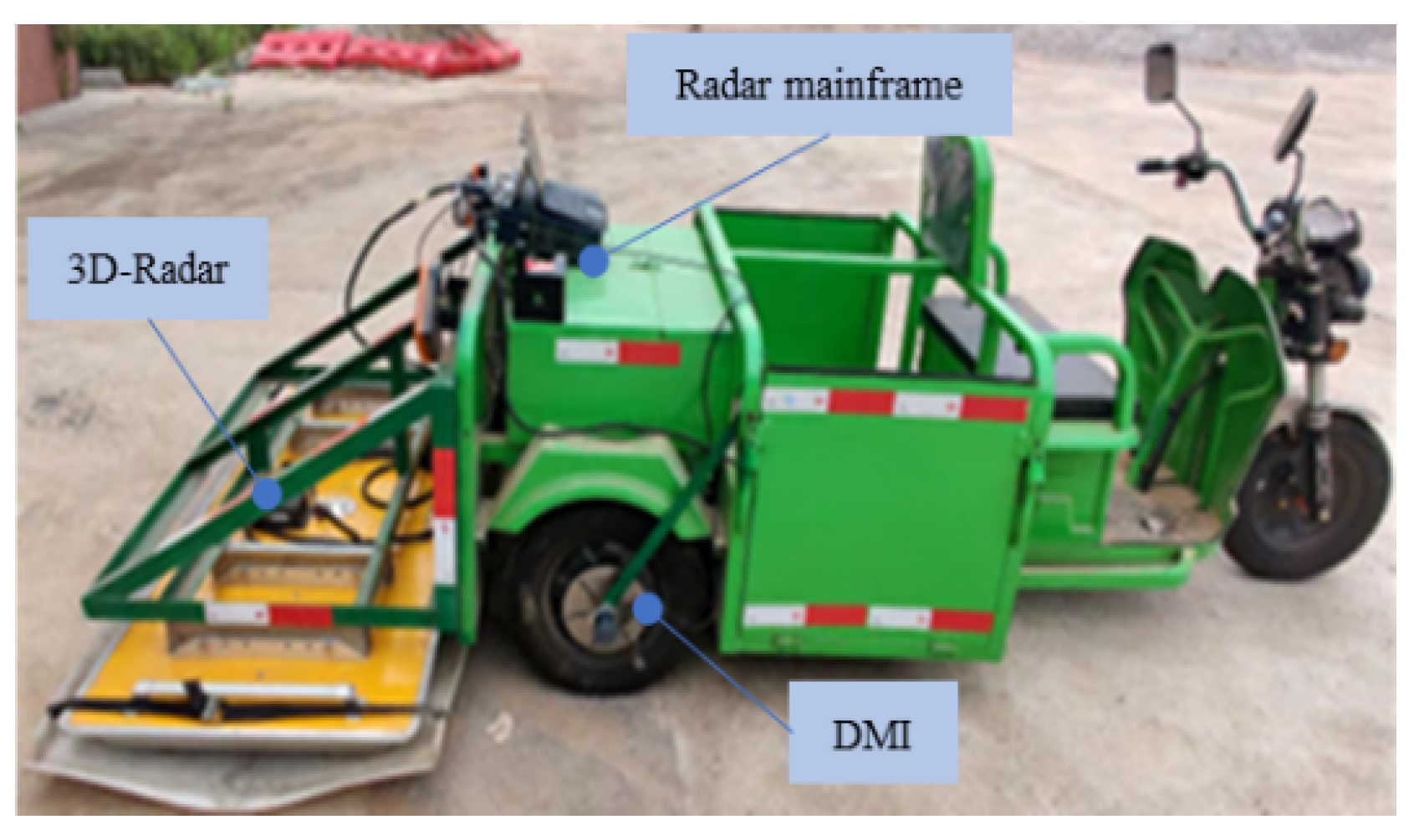
Remotesensing 15 03428 g008
Figure 9. GPR data acquisition equipment.
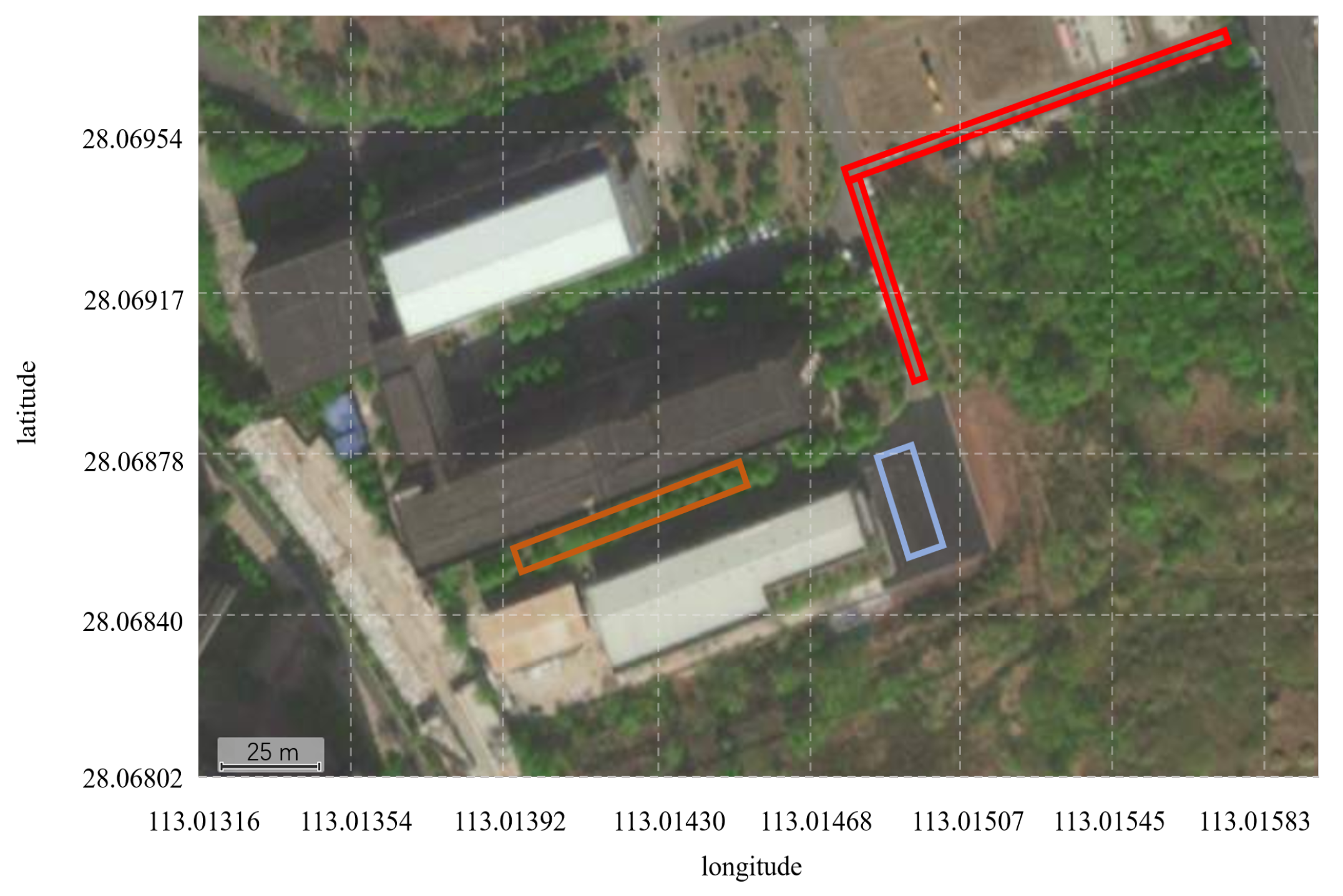
Remotesensing 15 03428 g009
Figure 10. Actual measurement data recording section schematic. Among them, the red, yellow, and blue boxes represent asphalt, masonry, and cement road sections, respectively.
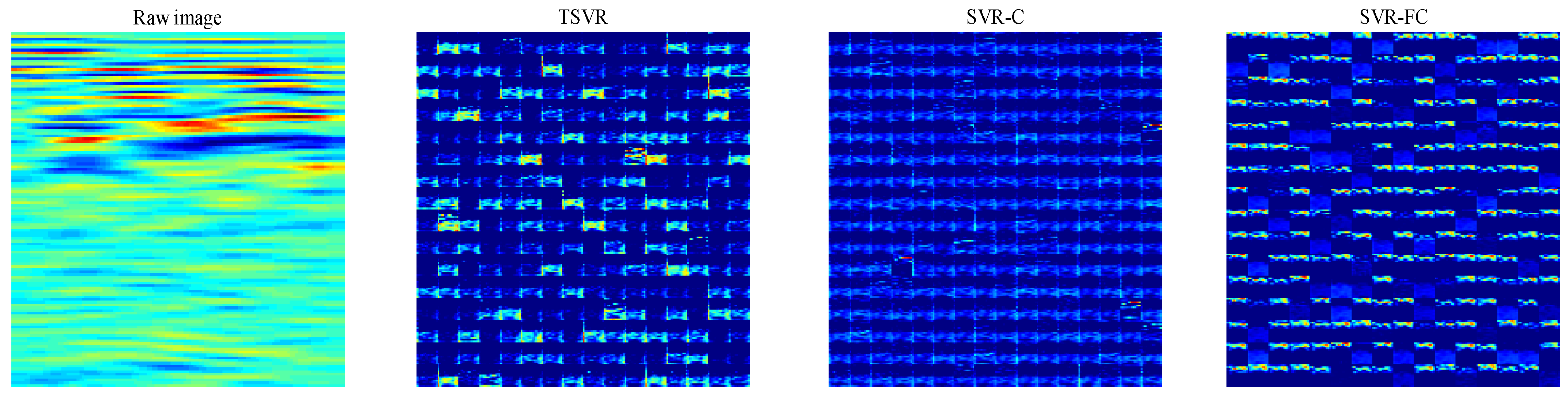
Remotesensing 15 03428 g010
Figure 11. Feature map visualization of the input conv3 layer. The left-most image is the input D-scan image. The following three images are the feature map collections of TSVR, SVR-C, and SVR-FC networks, respectively. Each feature map collection is obtained by arranging 256 feature maps in a 16 × 16 format.
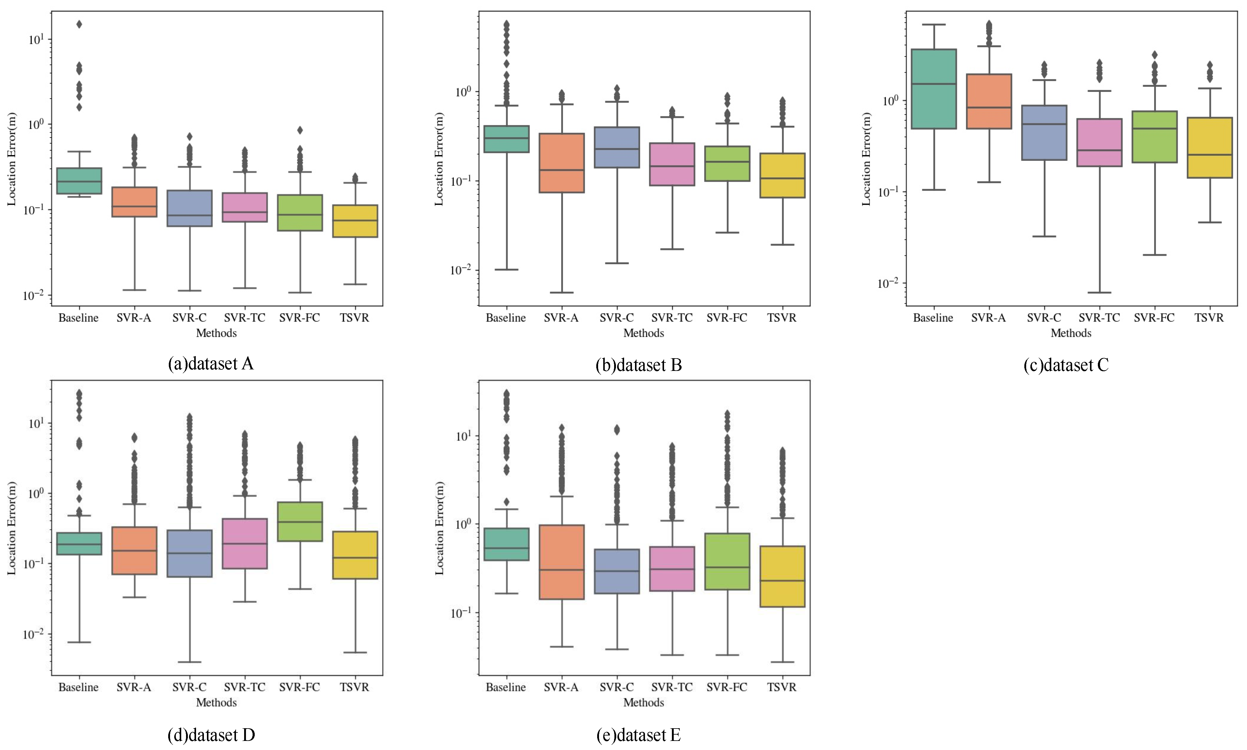
Remotesensing 15 03428 g011
Figure 12. Comparison of the localization errors under different localization methods. The results of comparing the localization errors of different methods on five datasets are shown in the figure. Each boxplot shows the six methods, baseline, SVR-A, SVR-C, SVR-TC, SVR-FC, and TSVR, from left to right. The statistical results for each method contain a median value line, a coloured box, upper and lower boundary horizontal lines, and several diamond-shaped discrete points. The horizontal line in the coloured box indicates the median value of the localization error. The upper and lower boundaries of the box indicate the 25th and 75th percentile, respectively, and the upper and lower black boundary transversals indicate the maximum and minimum errors after removing the discrete values, respectively. A cross-sectional comparison of each boxplot demonstrates the localization performance of different methods.
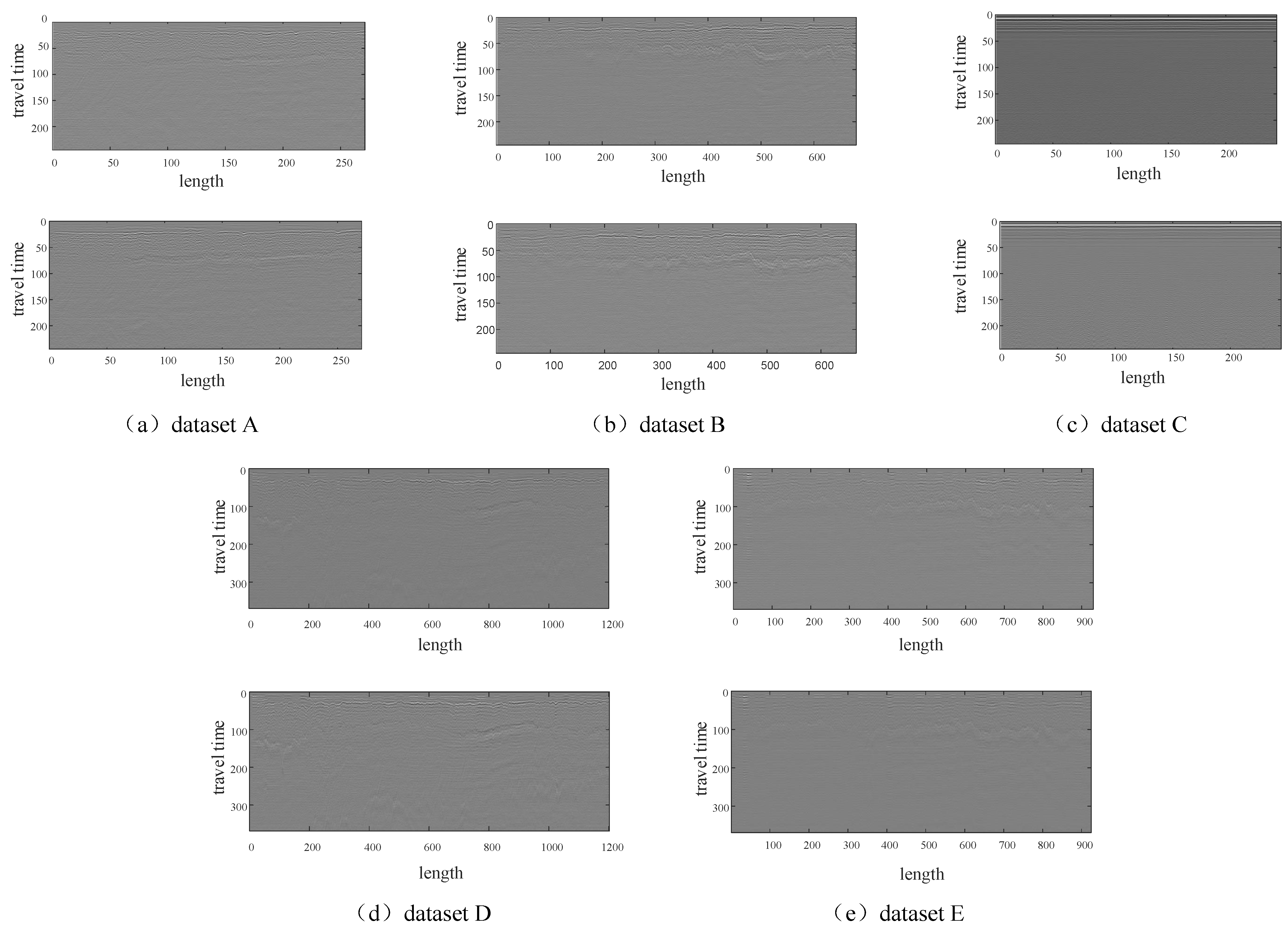
Remotesensing 15 03428 g012
Figure 13. B-scan images of the dataset. The two images of each dataset are the B-scan images of one channel extracted from the GPR data acquired at two different times. Among them, the volume data corresponding to the left image is used as the pre-collected map data, and the right image is used as the sliced data collected in real-time.
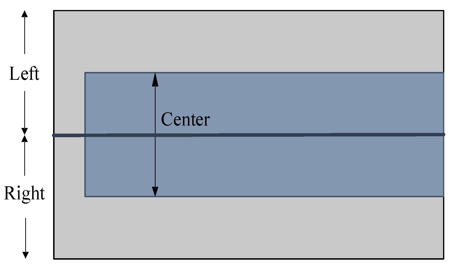
Remotesensing 15 03428 g013
Figure 14. Multi-lane mapping. (1) Left, (2) right and (3) centre. The left and right can be used to create a consistent map.
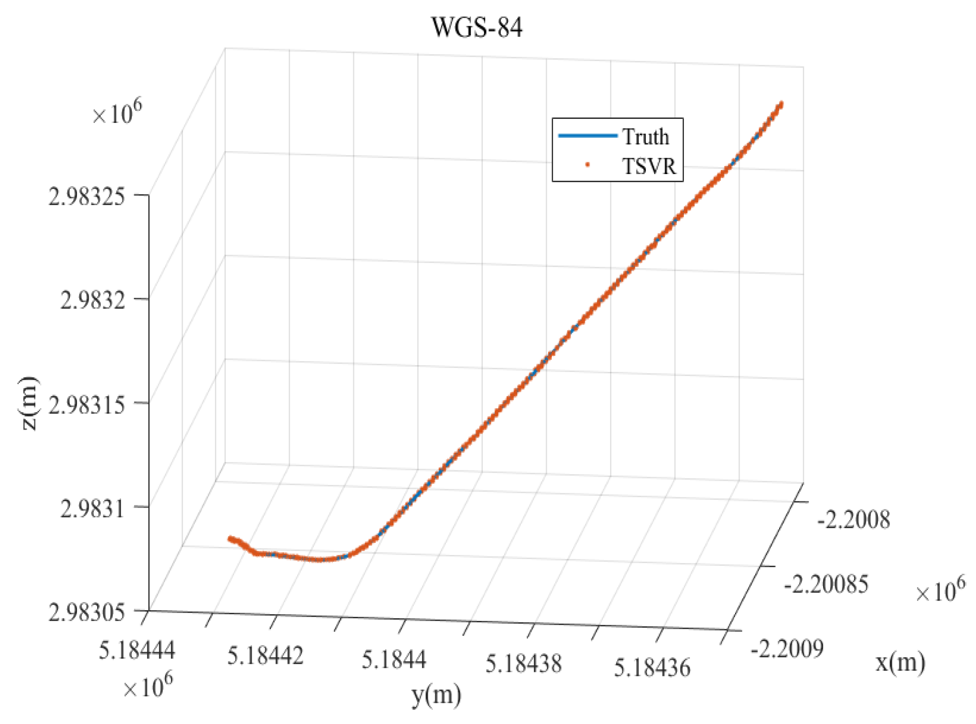
Remotesensing 15 03428 g014
Figure 15. Localization track of the TSVR method in the WGS-84 coordinate system.
Remotesensing 15 03428 g015
Table 1. GPR image frequency band correlation calculation.
Raw ImagesLow-Frequency ImagesHigh-Frequency Image
Correlation0.44600.68970.4211
Table 2. GPR system parameters.
ParametersParameter Values
Radar typeStepped frequency continuous wave
Frequency bandwidth2.8 GHz (200–3000 MHz)
Array dimensions1845 mm × 795 mm × 150 mm
Number of channels (number of pairs of elements)20
Elements spacing75 mm
Polarization modeLinear (scanning direction)
Sampling interval0.07 m
Detection depth2–3 m
Vehicle platform travel speed10 km/h
Table 3. Method descriptions.
MethodsSimilarity MeasuresOptimizer
BaselineNCCPSO
Average PoolingInput ImageInput FormatFeature ConcatenationAttention
SVR-AB-scan[227, 227, 1]
SVR-CD-scan[227, 227, 1]
SVR-TCB-scan, D-scan[227, 227, 2]
SVR-FCB-scan, D-scan[227, 227, 1] [227, 227, 1]
TSVRB-scan, D-scan[227, 227, 1] [227, 227, 1]
Table 4. Data description.
Road TypeWeatherLaneRoute_idLength
AsphaltClearLeft, centre, right1180 m
AsphaltRainCenter1180 m
MasonryClearLeft, centre, right260 m
MasonryRainCenter260 m
CementClearLeft, centre, right320 m
Table 5. Information entropy.
Asphalt (Clear)Asphalt (Rain)Masonry (Clear)Masonry (Rain)Cement (Clear)
entropy6.09096.08165.76034.87164.2013
Table 6. Metrics of the different methods under dataset A.
MethodsError Median (m)Error Var ( m 2 )
Baseline0.21341.4429
SVR-A0.10890.1699
SVR-C0.08550.1246
SVR-TC0.09380.0921
SVR-FC0.08710.1134
TSVR0.07450.0506
Table 7. Metrics of the different methods under dataset B.
MethodsError Median (m)Error Var ( m 2 )
Baseline0.30090.9654
SVR-A0.13260.2345
SVR-C0.22480.2190
SVR-TC0.14560.1410
SVR-FC0.16170.1415
TSVR0.10590.1686
Table 8. Metrics of the different methods under dataset C.
MethodsError Median (m)Error Var ( m 2 )
Baseline1.51662.0620
SVR-A0.82751.7316
SVR-C0.54480.5439
SVR-TC0.28480.5112
SVR-FC0.48820.5631
TSVR0.25280.4797
Table 9. Metrics of the different methods under dataset D.
MethodsError Median (m)Error Var ( m 2 )
Baseline0.18703.1185
SVR-A0.15100.6568
SVR-C0.13731.5713
SVR-TC0.18841.0519
SVR-FC0.38380.7729
TSVR0.12071.0784
Table 10. Metrics of the different methods under dataset E.
MethodsError Median (m)Error Var ( m 2 )
Baseline0.52786.7629
SVR-A0.30311.9535
SVR-C0.29221.1548
SVR-TC0.30731.4566
SVR-FC0.32352.0670
TSVR0.22681.2289
Table 11. Running time comparisons in CPU.
MethodsTime (per/s)
Baseline2.0955
SVR-A0.0230
SVR-C0.0234
SVR-TC0.0244
SVR-FC0.0298
TSVR0.0273
Disclaimer/Publisher’s Note: The statements, opinions and data contained in all publications are solely those of the individual author(s) and contributor(s) and not of MDPI and/or the editor(s). MDPI and/or the editor(s) disclaim responsibility for any injury to people or property resulting from any ideas, methods, instructions or products referred to in the content.

