Article

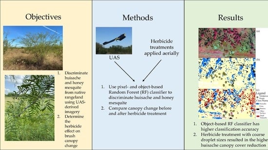
Identification of Brush Species and Herbicide Effect Assessment in Southern Texas Using an Unoccupied Aerial System (UAS)

1
Department of Soil and Crop Sciences, Texas A&M University, College Station, TX 77843, USA
2
Texas A&M AgriLife Extension Service, Uvalde, TX 78801, USA
3
Department of Computer Science, Texas A&M University-Corpus Christi, Corpus Christi, TX 78412, USA
4
Department of Agricultural and Environmental Sciences, Tennessee State University, Nashville, TN 37209, USA
5
Texas A&M AgriLife Research, Beeville, TX 78102, USA
*
Author to whom correspondence should be addressed.
Remote Sens. 2023, 15(13), 3211; https://doi.org/10.3390/rs15133211
Submission received: 10 April 2023 / Revised: 24 May 2023 / Accepted: 14 June 2023 / Published: 21 June 2023
(This article belongs to the Special Issue Monitoring Crops and Rangelands Using Remote Sensing)

Abstract

:
Cultivation and grazing since the mid-nineteenth century in Texas has caused dramatic changes in grassland vegetation. Among these changes is the encroachment of native and introduced brush species. The distribution and quantity of brush can affect livestock production and water holding capacity of soil. Still, at the same time, brush can improve carbon sequestration and enhance agritourism and real estate value. The accurate identification of brush species and their distribution over large land tracts are important in developing brush management plans which may include herbicide application decisions. Near-real-time imaging and analyses of brush using an Unoccupied Aerial System (UAS) is a powerful tool to achieve such tasks. The use of multispectral imagery collected by a UAS to estimate the efficacy of herbicide treatment on noxious brush has not been evaluated previously. There has been no previous comparison of band combinations and pixel- and object-based methods to determine the best methodology for discrimination and classification of noxious brush species with Random Forest (RF) classification. In this study, two rangelands in southern Texas with encroachment of huisache (Vachellia farnesianna [L.] Wight & Arn.) and honey mesquite (Prosopis glandulosa Torr. var. glandulosa) were studied. Two study sites were flown with an eBee X fixed-wing to collect UAS images with four bands (Green, Red, Red-Edge, and Near-infrared) and ground truth data points pre- and post-herbicide application to study the herbicide effect on brush. Post-herbicide data were collected one year after herbicide application. Pixel-based and object-based RF classifications were used to identify brush in orthomosaic images generated from UAS images. The classification had an overall accuracy in the range 83–96%, and object-based classification had better results than pixel-based classification since object-based classification had the highest overall accuracy in both sites at 96%. The UAS image was useful for assessing herbicide efficacy by calculating canopy change after herbicide treatment. Different effects of herbicides and application rates on brush defoliation were measured by comparing canopy change in herbicide treatment zones. UAS-derived multispectral imagery can be used to identify brush species in rangelands and aid in objectively assessing the herbicide effect on brush encroachment.

Graphical Abstract

1. Introduction

Identifying and monitoring noxious brush species is vital for landowners since the canopy cover percentage of different brush species could determine the necessity and method of brush management. There are two noxious brush species rapidly encroaching on coastal grasslands in southern Texas, namely, huisache (Vachellia farnesianna [L.] Wight & Arn.) and honey mesquite (Prosopis glandulosa Torr. var. glandulosa). Huisache is native to Texas and usually occurs where land is disturbed. It is a multi-stemmed shrub or tree typically less than 6 m tall but can be greater than 10 m occasionally [1]. When huisache canopy cover is below 11%, brush competition with grasses is not considered a problem; however, when its canopy cover approaches 20%, there is vigorous competition with grasses for water and nutrients [2]. Research indicates less than 25% of mesquite canopy cover causes little impact on warm-season mid-grass production, and when canopy cover is less than 30%, honey mesquite does not impact cool-season grass production [3]. So, 25% of mesquite canopy cover and 20% huisache canopy cover can be set as the threshold rangeland managers use to determine when treatment is necessary for optimum forage production. As one of the most effective management methods, chemical treatment has been a primary means of brush management in the southern U.S. for decades [4]. The plant physiology and growing conditions, herbicide selection, spray mix, and nozzle selection are heavily related to the success of herbicide applications.
Remotely sensed images have a long history of being used to identify different types of land cover [5,6,7,8]. If land managers want to be aware of the canopy cover and location of noxious brush over time to improve management decisions, an Unoccupied Aerial System (drone plus sensor payload; UAS) is a useful tool due to its higher efficiency than manual ground truth and provides a broader view of the entire land area at a field scale. Since noxious brush locations are stationary and present for long time periods even after treatment, utilizing UAS to track the temporal change in brush species is viable throughout several years. Compared to conventional remote sensing images from satellite or airborne platforms, UAS can be deployed quickly and repeatedly and with more flexibility to avoid bad weather and cloud cover, which facilitates temporal studies [9]. Using UAS for agricultural purposes is advanced and practical when only a limited land area is studied [10]. Field scale usually requires space- or air-borne platforms since UAS can fly up to 122 m (400 ft) altitude above ground level and can cover areas ranging from 8 to 500 ha based on UAS type such as fixed-wing or rotor-copter and based on different application purposes [11]. A UAS equipped with small-format digital red–green–blue (RGB) cameras or multispectral sensors for discrimination of plant species composition should be methodologically scrutinized and the classification progress combined with additional UAS imagery-derived products such as vegetation index added to the input [12].
Prior work has considered utilizing a UAS equipped with multispectral sensors to assist in rangeland management [13,14,15]. Gillian et al. used a UAS to collect multispectral images over northern California to estimate rangeland indicators: fractional cover, canopy gaps, and vegetation height. They also evaluated the logistics framework of integrating UAS into an existing rangeland monitoring program. When they compared the UAS-derived results with field-collected results, fractional cover achieved high agreement (R2 = 0.77), while the canopy gaps and vegetation height had subpar agreement. They conclude that a UAS could be a standard tool for rangeland inventory and monitoring [16]. Laliberte et al. conducted a study in southern New Mexico to compare the classification results on rangeland using space-borne and UAS-borne multispectral image with object-based classification over Random Forest classifier. They found that multispectral images collected by UAS provided higher classification accuracy on Sumac, Creosote, Mesquite, and Tarbush [17]. Jackson et al. compared the classification results with different flying altitude over noxious plant honey mesquite and yellow bluestem in south Texas, and the Random Forest (RF) classifier outperformed other models tested in the study. His study also suggested that flying altitude at approximately 100 m is most suitable for mapping honey mesquite [18]. The herbicide effect of noxious brush has not been evaluated by UAS equipped multispectral imagery before. Current ratings of herbicide efficacy are subjective in nature and made by a trained observer, and using imagery could provide a more objective measure.
Even though Random Forest classifier has been proved to have good performance over landcover mapping research, a comparison of the object- and pixel-based classification result with RF has not been performed on noxious brush before. The RF classifier has been previously used on satellite image NDVI and Lidar data to map mesquite in south Texas [15]. Multispectral images and NDVI data have been tested for RF classification on mesquite and yellow bluestem [18]. This earlier work neither compared other band combinations nor evaluated the pixel-based classification method to determine if it was more applicable on brush species. Machine learning algorithms have been reported as a useful tool for monitoring various aspects of crops and plant species [19,20,21,22]. RF classifier uses numerous binary decisions to determine the classification of an image. When dealing with multi-source and multi-dimensional data, RF is often selected [23]. RF classification algorithms can be both used as pixel-based and object-based classification. Pixel-based classification is performed on a per-pixel level, and it uses available spectral information for that individual pixel. Object-based classification aggregates image pixels into objects that are spectrally homogenous and then classifies them over individual objects. Object-based classification can provide context and shape information, which are not provided by pixel-based classification, to the classification process [24]. Knowing the ‘neighbors’ and the spatial and spectral relations with and among objects gives object-based classification better results than pixel-based classification [25]. RF with ideal model parameters performs well among other classification algorithms [26,27]. Another advantage that RF has compared to other commonly used classification methods is the use of bootstrapping and a random subset of sampling strategy when building the RF model [26,28].
Mapping brush species encroachment at the field level is necessary for land management decisions for herbicide application and other decisions. UAS-derived imagery classification can be a useful tool to map brush species and determine objective measures of herbicide efficacy; however, the herbicide effect of noxious brush has not been evaluated with multispectral imagery collected by UAS. Band combinations other than multispectral and NDVI have not been compared previously, nor have pixel- and object-based methods been compared, for discrimination and classification of noxious brush species with RF. In this research, we aim to estimate the canopy change in encroaching huisache and honey mesquite to assess the effect of different herbicide treatments on rangelands in south Texas. The main objectives of this study are to (i) discriminate huisache and honey mesquite from native rangeland using the RF classification method to compare object- and pixel-based classification; and (ii) determine the herbicide effect on the brush post-herbicide application. The hypothesis is that the RF classification using UAS equipped with a multispectral sensor imagery can identify the two brush species in rangeland.

2. Materials and Methods

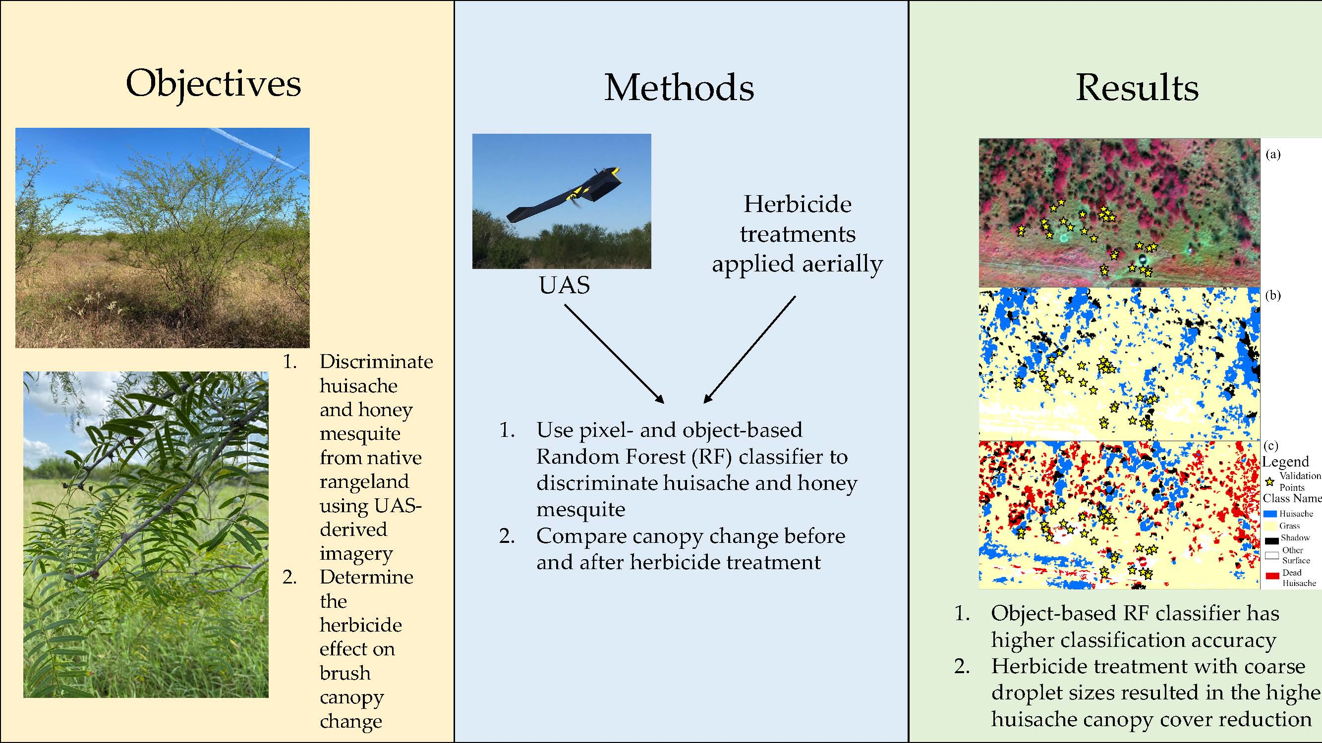
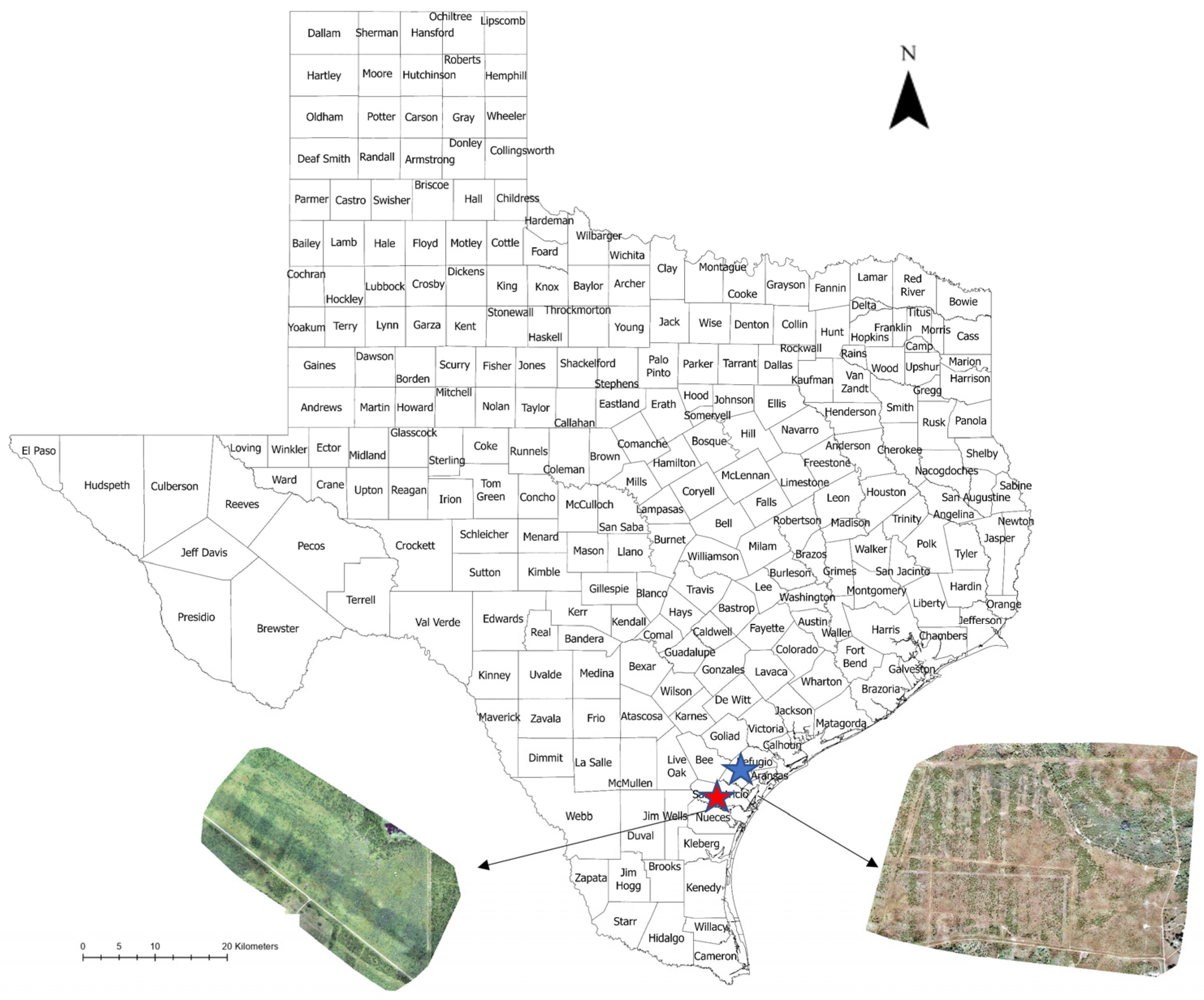
2.1. Rangeland Information

This research was conducted at two private ranches in Refugio (Site 1) and San Patricio (Site 2) Counties, Texas. The geographic location of Site 1 was 28°40′49.440″N, −97°17′12.780″W, and the site was around 30 m above sea level. The geographic location of Site 2 was 28°41′2.18″N, −97°17′1.69″W, and the site was around 13 m above sea level. Site 1 is characterized by Papalote Fine Sandy Loam (0–1% slopes), Banquete Clay (0–1% slopes), and Orelia Fine Sandy Loam (0–1% slopes) soils. Site 2 consisted of Calallen Sandy Clay Loam (0–1% slopes) and Victoria Clay (0–1% slopes) soil series. Both sites had brush encroachment by huisache and honey mesquite, although huisache was the dominant species at Site 1. The location of both sites is shown in Figure 1.

2.2. Data Acquisition

An eBee X fixed-wing UAS (SenseFly, Cheseaux-sur-Lausanne, Switzerland) with a Parrot Sequoia multispectral camera (SenseFly, Cheseaux-sur-Lausanne, Switzerland) and built-in 16 MP RGB camera, part of the multispectral sensor, was used to collect data. The spectral range of the multispectral camera is Green (550 nm ± 40 nm), Red (660 nm ± 40 nm), Red Edge (735 nm ± 10 nm), and Near-infrared (790 nm ± 40 nm). The ground sample distance (GSD) of this camera at 120 m above ground level is 11 cm per pixel. Two separate flight missions were conducted both at Site 1 and Site 2. The flying altitude was 100 m in approximately 10 cm resolution, and the flight overlap was 90%, with six ground control points used. At each flight, a downwelling light sensor was used to capture the sun radiation. It recorded the light conditions during the flight, so when pre-processing the images, software such as Pix4D can be used to normalize images captured in different illumination conditions. The flight coverage over Site 1 mapped 0.82 km2, and over Site 2 it mapped 0.43 km2.
On 15 November 2019, Site 1 was treated aerially with herbicide to suppress or control the huisache. On the same day, a pre-herbicide image was collected. There were two purposes of this spray, namely, testing droplet size and herbicide efficacy. Table 1 summarizes all treatments. For testing droplet size, herbicide treatments were the same. Two droplet sizes of 400 μm and 800 μm were used; each droplet size included two rates of herbicide mixture volume, 37.4 L ha−1 and 74.8 L ha−1. For each droplet size and rate, two replications were included (Table 1, treatment 1–7, 13). For brush suppression purposes, five treatments were made with no replications, and each treatment had different herbicide combinations (Table 1, treatment 8–12). The suppression treatments used the same flat fan nozzles. All treatments were applied at 10–20 PSI. On 11 November 2020, a post-herbicide image of Site 1 was collected with the same methods as in 2019. After the initial herbicide application in 2019, no other brush control treatments were applied to Site 1.
At Site 2, two images were collected on 26 June 2017 and 26 July 2021; they were both post-herbicide applications because the herbicide was applied on 29 October 2014. After 2014, no chemical treatments were applied to this site, and no pre-herbicide image was collected, so long-term herbicide effect can be measured based on the images collected in 2017 and 2020. The herbicide application at Site 2 used the same herbicides, predominately aminocyclopyrachlor, at the same rate, but the rate was not recorded (Table 2). Droplet size (417 μm, 630 μm, or max) and application rates (37.4 or 86.8 L ha−1) were varied in four treatments. One replication for each treatment was within the experiment site. Figure 2 showed the location and distribution of herbicide treatment in both sites. Treatment numbers in Figure 2 represent the numbers in Table 1 and Table 2.

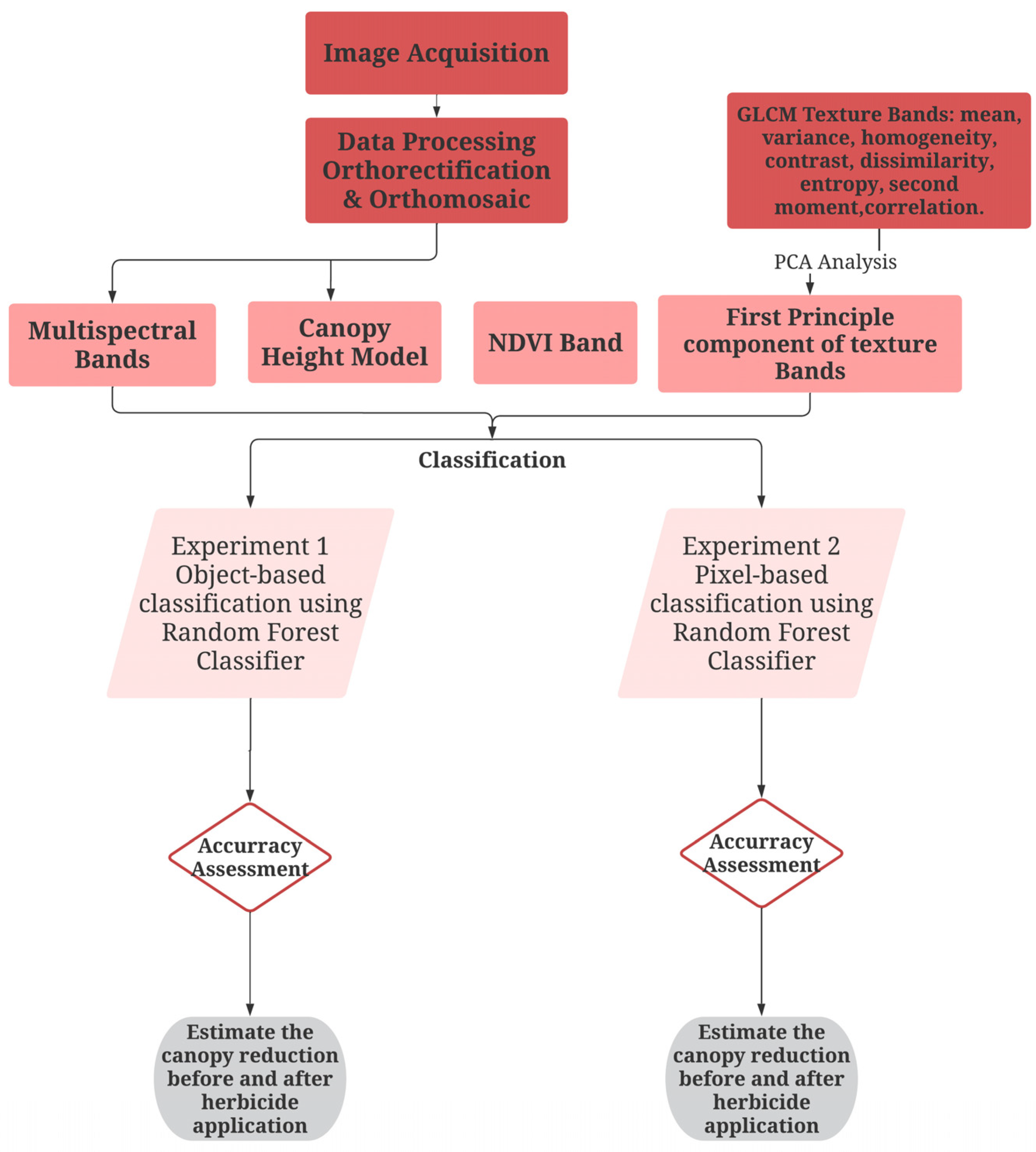
2.3. Data Processing

Data Processing and analysis workflow is shown in Figure 3. After data acquisition, images were processed in Pix4D for georeferencing, spatial alignment, and orthorectified mosaic. The orthorectified images of different dates had a slight co-register issue, so manual co-registration was performed in ArcGIS Pro. In Pix4Dmapper, 3D point cloud was generated from the RGB data using structure-from-motion (SfM) photogrammetry and then used to generate Digital Surface Model (DSM). We were unable to generate a Digital Terrain Model (DTM) of the bare-earth surface because the high vegetation cover in all sites caused very little exposed ground to collect ground elevation. Instead of using a UAS-derived DTM, the USGS National Map of 1 m Digital Elevation Model collected on 11 November 2018 was used (USGS, 2018) as ground elevation. The DTM is a tiled collection of the 3D Elevation Program (3DEP) collected by nationwide Lidar with one-meter resolution. The DTMs for two sites were georeferenced and resampled to the multispectral image’s extent and resolution. After generating appropriate DTMs from the USGS products, Canopy Height Model (CHM) was generated by subtracting DTM from DSM.
To better assess the brush classification, ground truth points and visual interpretation indicated mesquite and huisache had texture differences, in that mesquite had coarser leaves than huisache. So, Gray-Level Co-Occurrence Matrix (GLCM) texture analysis was conducted on both sites’ data, in which eight statistics were automatically computed with a 3 × 3 moving window. The statistics were contrast, correlation, variance, entropy, second moment, homogeneity, mean, and dissimilarity. Principle Component Analysis (PCA) was conducted on the eight statistical bands from GLCM analysis to reduce the dimensionality issue when stacking bands, and the first PCA band out of eight bands was selected. After generating all the bands, they were stacked together. Furthermore, to assess the effect of different bands, other band combinations were also tested and summarized in Table 3.
With different band combinations, the pixel-based (Experiment 1) and object-based (Experiment 2) classifications were conducted. Both experiments used an RF classification algorithm to compare pixel-based and object-based classification results. After classification, canopy reduction can be estimated based on classified images.

2.4. Training Sample Collection and Classification

The first step of object-based classification is to collect training data. For Site 1, there were 70 ground points matched with the visual interpretation of brush species to collect training samples. For each class, training samples used approximately 20% of pixel size out of the total training sample pixel size to maintain sample size balance. Ground truthing found little mesquite present at Site 1, so there were limited training samples available. To avoid breaking the training sample balance, the mesquite class was not included in Site 1. So, the training samples in Site 1 data collected in 2019 had four classes: huisache, shadow, other surfaces, and grass. The training samples in Site 1 data collected in 2020 had five classes: huisache, shadow, other surfaces, dead huisache, and grass.
For Site 2, we had 180 in situ ground points marked with RTK GPS and matched with visual interpretation to collect training samples. There were six classes in Site 2: huisache, mesquite, shadow, other surfaces, dead brush, and grass. For both sites, the collected data were split randomly with the subset features function at 80/20 percentage rate to create the 80% training and 20% testing dataset.
To perform object-based classification, a mean shift segmentation was used. From trial-and-error results, spectral details and minimum segment size in pixels were set to 20, spatial details were set to 15, the classification parameters over a segmented image used a maximum number of decision trees and a maximum number of samples per class set to 1000, and tree depths were set to 500. After classification, accuracy assessment used the create accuracy assessment points function and iterated 20 times with equalization stratified random method, which generates a set of accuracy assessment points. Then, the computing confusion matrix was run for each iteration, resulting in user accuracy, producer accuracy, and overall accuracy for individual classes. A standard deviation was estimated by multiplying accuracy error with accuracy and dividing by the number of samples and then taking a square root of the value. The standard overall accuracy refers to the ratio of the total correctly classified number of pixels to the total number of reference pixels; user’s accuracy refers to the ratio of correctly classified pixels of a given class to all pixels classified in this category; producer’s accuracy refers to the ratio of correctly classified pixels to all pixels in the set of validation data for this class [29]; precision measures how many of the positive predictions made are correct; recall measures how many of the positive samples the classifier correctly predicted [30]. Pixel-based classification followed a similar workflow with the same parameters for RF classifier, except there was no segmentation imagery as input. After classification, canopy cover change was calculated for the living and dead brush within the herbicide spray area by counting the pixel numbers of the regions per class with standard deviation generated automatically. This facilitated measuring the herbicide effect on the brush species.

3. Results

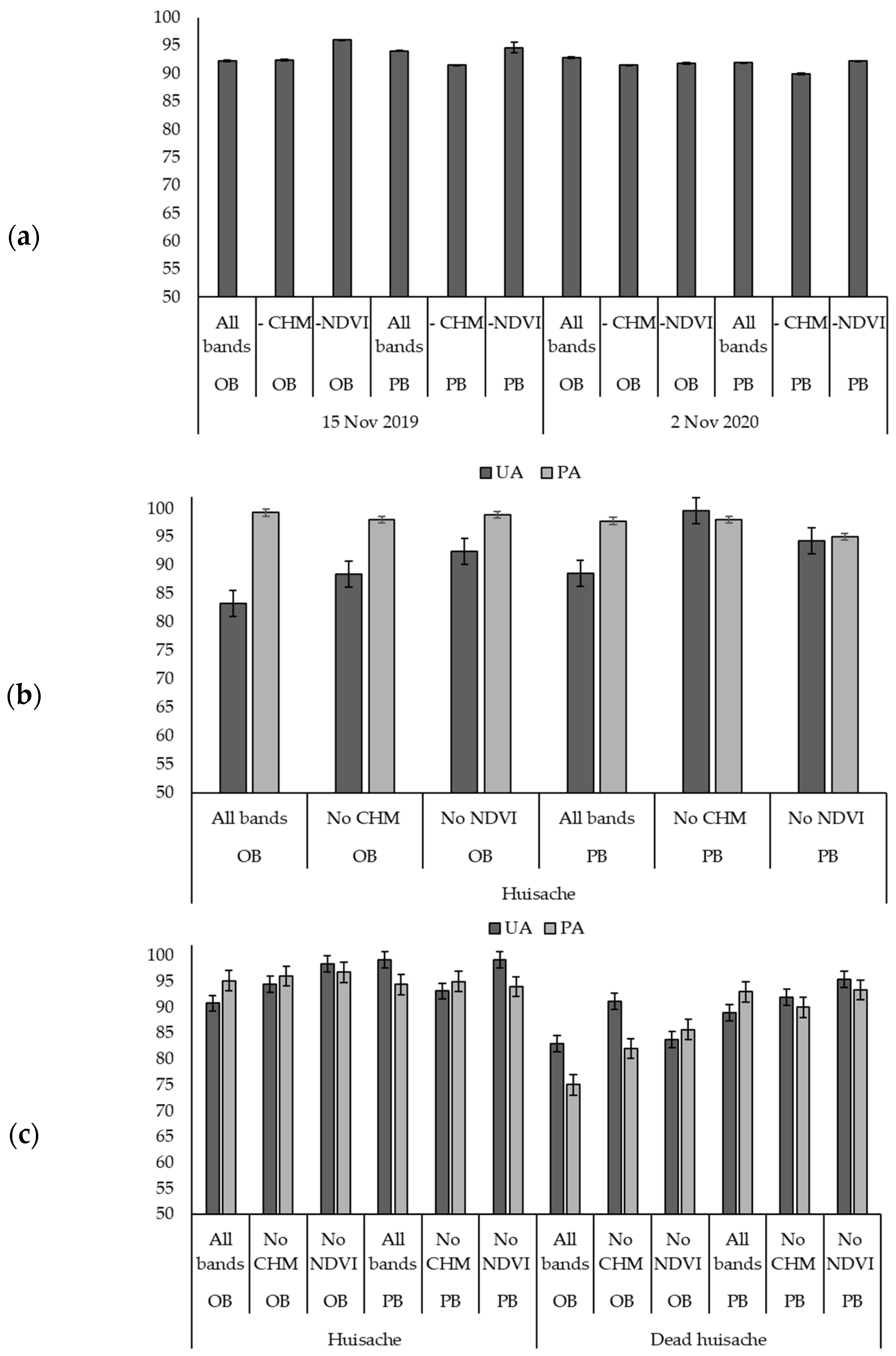
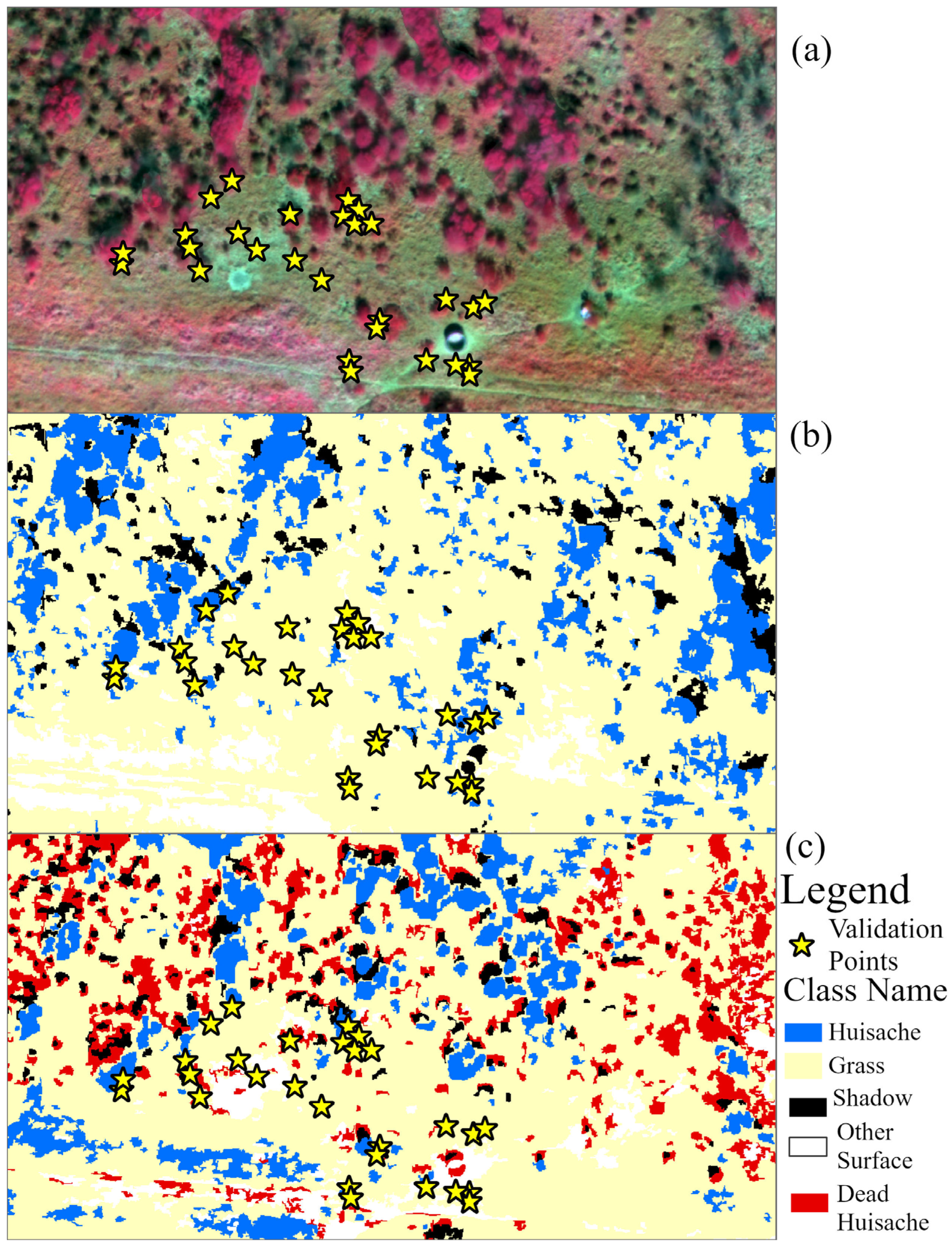
3.1. Results of Site 1

3.1.1. Brush Classification

The classification results before herbicide treatment in 2019 are shown in Figure 4, along with the classification results one year after herbicide spray in 2020 including dead huisache.
When all bands were applied to classification, the brush was distinctly separated from grass and other surfaces. Experiment 1, which applied object-based classification over RF classifier, and Experiment 2, which applied pixel-based classification over RF classifier, showed similar results (Figure 4). The classification results for data collected in 2020 had a cluster of dead huisache in the center of Site 1. Since the herbicide applications appeared to be more effective in the center, and other classes were accurately classified, the overall accuracy affected the user’s and producer’s accuracy in the dead huisache class (Figure 4), which indicated consistency during classification using different classification methods.
When all bands except for NDVI were applied to classification, object- and pixel-based classification showed similar results and similar overall accuracy (Figure 4). For data collected in 2019, object-based classification did not separate shadow from plants well since NDVI is used to identify the presence of vegetation. Adding CHM to the model and removing NDVI in 2020 data still showed the cluster of dead huisache, indicating CHM was producing this result and not NDVI. In pixel-based classification, there was some misclassification between dead huisache and grass because the herbicide application suppressed some huisache, leading to partially defoliated huisache remaining rather than total defoliation. Without NDVI to identify the vegetation, misclassification inevitably occurred.

3.1.2. Herbicide Efficacy Assessment

Table 4 compares the brush canopy cover percentages over the entire site in 2019 and 2020. The brush canopy change was affected by herbicide treatment, so the brush canopy change was compared to the untreated area. Table 5 compares the brush canopy cover percentage within individual herbicide treated areas in 2019 and 2020. All the bands combined can assist in identifying brush canopy in 2019, and removing the CHM combination was more suitable for data collected in 2020. Grass was often misclassified as brush because of the similar spectral profiles and lack of CHM to differentiate the height difference. This inferred grass canopy cover ranged from 50% to 70% in 2019 and 30–50% in 2020. Shadow and other surfaces only accounted for less than 10% of cover individually. Therefore, in Site 1, most of the cover came from grass and noxious brush. After herbicide treatment, huisache canopy was composed of 15–20% cover, which is near the threshold of 20% where management is usually needed, but canopy cover had decreased by 10% across the whole site when comparing pre- and post-herbicide treatment huisache canopy cover. Within the herbicide treated area, different treatments resulted in different defoliation levels of huisache canopy cover change (Table 4).
Applications with spray volumes of course droplet sizes (Treatments 1, 4, 5, and 13) resulted in the highest huisache canopy cover reduction of 30–65%. Two treatments, MezaVue® (Treatment 11) and Grazon Next HL® + Tordon® + MSM 60® (Treatment 12) had increased huisache canopy cover change, even more than 100%. To assess these abnormal canopy change findings, multispectral imagery was used to identify the two treatment areas. Huisache defoliation was not observed in regions of Treatment 11, and huisache leaves became coarser in multispectral imagery. However, treatment 12 did show huisache defoliation from visual interpretation between pre- and post-treatment imageries, and it is possible that grasses were misclassified to huisache, causing the canopy cover increase. This indicated that the canopy change in treatment 12 region was unrealistic, and more field validation of this area was desired. The comparison between field validation data and best-performing classification results gives more uncertainty to the findings since the validation accuracy reached less than 70%.
Based on classification results in Site 1, object-based classification applied to multispectral bands, NDVI, and the first-principal component of GLCM bands achieved the best classification results. To further validate the results, field validation points of huisache locations were overlayed with classification results using such band combinations and object-based classification (Figure 5). From the points located, we can tell some field validation points for huisache were marked at the edge of the huisache. However, the classification results mostly preserved the central shape of huisache, though some points marked at the plant’s edge were not correctly classified. Some ground truth points were marked on small huisache less than 1.9 m. These were not all accurately classified because the short and young huisache leaves displayed a similar spectral profile with grasses. Out of 55 huisache validation points, object-based classification using all bands, but not CHM, had 31 correctly classified points (56.36% accuracy) in 2019 and 37 correctly classified points (67.27% accuracy) in 2020. With previous observation of validation point positions, low accuracies were expected.

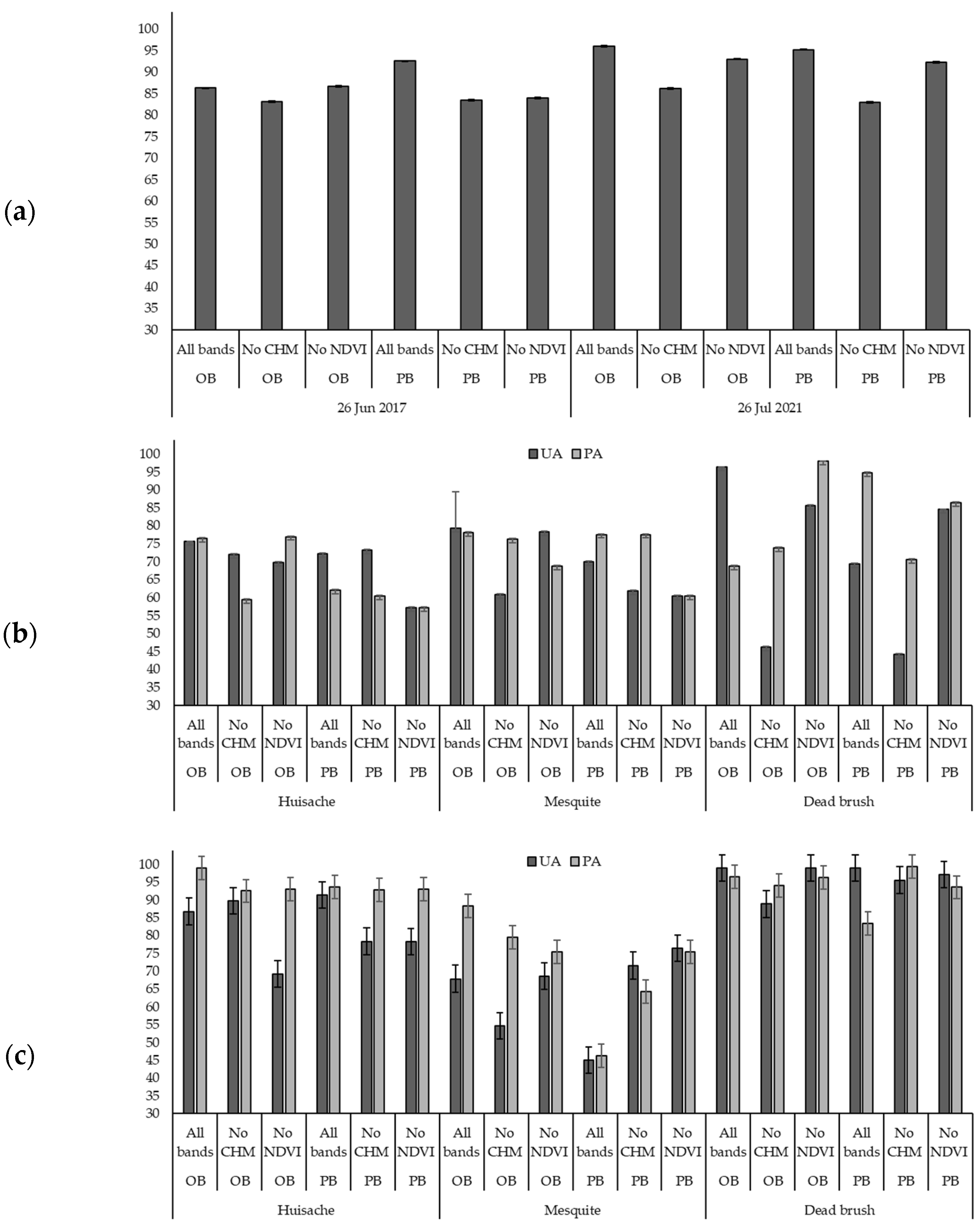
3.2. Results of Site 2

3.2.1. Brush Classification

As opposed to Site 1 which was dominated by huisache, Site 2 had a combination of both mesquite and huisache. Since the herbicide application was completed before the first flight in 2017, only the long-term herbicide effect was assisted by classification results. Classification results are shown in Figure 6. The highest accuracy (96%) was found when using all bands with the object-based classification method (Figure 6). Object-based classification typically had better overall accuracy than the method used for pixel-based classification. Mesquite and grass had relatively low user’s accuracy, especially without CHM, since mesquite misclassified with grass easily. Overall, the object-based classification with all bands generated a high overall accuracy and user’s accuracy.
Overall, object-, and pixel-based based classification showed similar species identification of brush. Moreover, with functional CHM, stacking all bands together resulted in a more accurate classification of brush. At Site 2, object-based classification applied to all multispectral bands, NDVI, CHM, and the first-principal component of GLCM bands achieved the best classification results. To further validate the results, field validation points of huisache locations were collected in 2021 and overlaid with classification results using such band combinations and object-based classification. Part of the points overlayed with multispectral imagery and classification results are shown in Figure 7. From the point locations, it is obvious some field validation points for huisache were marked at the edge of the plant, similarly to what was observed in Site 1. Out of 83 huisache validation points, object-based classification using all bands had 47 correctly classified points (54.22% accuracy) in 2017 and 61 correctly classified points (73.49% accuracy) in 2021. Some huisache that appeared dead in 2017 re-grew or added new plants by 2021, so the later validation points were not as reliable for validating 2017 results.

3.2.2. Herbicide Efficacy Assessment

Table 6 compares the brush canopy cover percentages over the entire site in 2017 and 2021. The brush canopy change was affected by herbicide treatment, so the brush canopy change was compared to the untreated area. Table 7 compares the brush canopy cover percentage within individual herbicide treated areas in 2017 and 2021. Huisache and mesquite on Site 2 exhibited different growth patterns. In 2017, mesquite canopy cover ranged from 12 to 18%, which indicated that mesquite at Site 2 likely had little impact on the warm-season grass production [31]. However, in 2021, mesquite canopy cover increased to around 20 and 30%, nearing or reaching the threshold of 30% for competition with both warm- and cool-season grass production [31]. Within the herbicide-treated area, mesquite increased in canopy cover by over 200%, likely due to the reduced competition with huisache since the herbicide application timing was targeted to huisache and not mesquite (Table 7).
For huisache at Site 2, there was approximately 20% canopy cover in 2017, which met the threshold for competition with grasses [3] (Table 6). Since herbicide had been applied before 2017, the huisache canopy change due to the herbicide application cannot be assessed quantitatively but can be compared with adjacent, untreated areas. Since the timing of the herbicide application was specifically targeting huisache, we know that even three years after herbicide application, the overall huisache canopy cover on the site was still above the threshold for grass competition, and additional herbicide application on the untreated strips may be warranted. All treatments used the same chemical Aminocyclopyrachlor mixture with different droplet size and application rate. A small droplet size with a low application rate (Treatment 1) and a large droplet size with a high application rate (Treatment 4) had better control of huisache, with 10% and 20% huisache canopy reduction maintained, respectively, while a small droplet size with a high application rate (Treatment 2) and a medium droplet size with a high application rate (Treatment 3) had an increase in huisache canopy cover of over 100%. Overall, huisache did increase in the treated area during the 4 years of the UAS data collection. Still, compared to the unsprayed areas, the long-term herbicide effect seven years after application demonstrated a drastic reduction in huisache cover.

4. Discussion

4.1. Classification Results Comaprison

The main objective of this study was to identify huisache and honey mesquite and to determine if brush classification maps could be used to measure herbicide efficacy of these brush species. Huisache and mesquite were identified with UAS-collected multispectral imagery and multispectral imagery-derived phenotypic data such as NDVI, CHM, and GLCM bands. At Site 1 (Figure 4), the highest accuracy was from the model without NDVI, whereas at Site 2 (Figure 6), the highest accuracy was from applying the classifier on all bands. When comparing the classification map of stacking all bands and the model without NDVI, stacking all bands had slightly better performance. However, if available features were to cause multicollinearity, the NDVI band could be removed. In this research, CHM was vital for discriminating brush from grass, so the compromised CHM at Site 1 could not generate the best classification result. Object-based classification had better results than pixel-based classification since pixel-based classification tended to overestimate classes with a ‘salt-and-pepper’ effect.

4.2. Herbicde Effect on Brush Species

In this research, object-based classification with all bands, excluding CHM, added to classification input and achieved the best result at Site 1. Several herbicide treatments were found to have the potential to control brush invasion in the short-term based on classification and canopy change results. In Site 1 (Table 4 and Table 5), herbicide treatment with coarse droplet sizes (Treatment 1, 4, 5, and 13) resulted in the highest huisache canopy cover reduction, 30–65%. Other treatments using fine droplet sizes (Treatments 2, 3, 6, and 7), DuraCor® (Treatment 8), DuraCor® + Chaparral® (Treatment 9) and DuraCor® + MezaVue® (Treatment 10) resulted in an overall huisache canopy cover reduction of 10–30%. Two treatments, MezaVue® (Treatment 11) and Grazon Next HL® + Tordon® + MSM 60® (Treatment 12), had an increase in huisache canopy cover one year after treatment of more than 100%. Field validation data of huisache apparent liveness within the treated area can be used to validate the results.
In Site 2 (Table 6 and Table 7), the measurements of canopy change are from 3 years and 7 years after herbicide treatment. A small droplet size with a low application rate (Treatment 1) and a large droplet size with a high application rate (Treatment 4) had a higher canopy cover reduction, approximately 10% and 20%, respectively, while a small droplet size with a high application rate (Treatment 2) and a medium droplet size with a high application rate (Treatment 3) had an increase in huisache canopy cover of over 100%. Site 2 was treated with herbicide more than 7 years before data acquisition, demonstrating the herbicide treatments did control the brush long term when compared to the adjacent, untreated areas at the site. The increase in mesquite cover from year 4 to year 7 post-herbicide application was likely due to the control of huisache, resulting in open canopy space and less competition for mesquite. Management decisions of one brush species should consider the dominant botanical composition of the rangeland, especially in the case of huisache and mesquite since they typically must be treated at different times of the year. Overall, huisache was controlled within the treated area compared to the untreated areas. After validating the classification accuracy, the canopy change for brush species can be a great indicator of when follow-up treatments might be necessary.

4.3. Relevent Work Comparison

The results from this study are comparable to similar studies. Previous work in south Texas compared the classification results with different flying altitude over noxious plant honey mesquite and yellow bluestem in south Texas, and the object-based RF classifier outperformed other models tested in the study [18]. The previous study also suggested that flying altitude at approximately 100 m is most suitable for mapping honey mesquite [18]. The highest overall accuracy of mapping mesquite is 87% for flying altitude at 100 m in April, which was lower than this study. They used NDVI, and no plant height features were considered. In 2019, another study used less than 1 m NAIP satellite imagery and Lidar data to map mesquite above ground biomass [15]. They used object-based RF to test combining National Agricultural Imaging Program (NAIP) with Lidar images or mapping mesquite separately with NAIP and Lidar data, and they did not report the accuracy of the study but presented the pseudo-coefficient of determination (R2). Combining NAIP and Lidar data gave the highest R2, but it was only 0.37, which reflects that the mapping classification was not ideal [15]. There is a paucity of information on mapping huisache using remote sensing data in recent years. Previous studies tended to use aerial photos to assess the spectral profile of brush species [13]. Plant canopy spectral-radiometric reflectance measurements, aerial photographs, and ground truth observations have been used to observe the huisache canopy reflectance [13]. Huisache reflectance was only distinguishable on conventional color (0.40 to 0.70-um) when flowering, but on CIR and aerial photo, it could not be distinguished even though they collected data in June, July, and September, due to photogrammetry limitations at that time [13]. Another study [32] found similar canopy reflectance of huisache, wherein they found the best date to distinguish huisache was when huisache is flowering in the spring. These findings suggest the best time to distinguish huisache and mesquite is the springtime when huisache is flowering. This study has also expanded the exploration to map huisache on rangeland using a machine learning approach with high resolution aerial images.

4.4. Limitations and Further Directions

For brush classification, a high-quality and reliable height model of the experiment site is crucial for better classification. For further research, more extensive processing of DSM and DTM can be considered to reduce errors when creating CHM. A UAS-Lidar system could also be useful to explore improved CHM since it can assess below vegetation elevation better than the structure from motion techniques used in this experiment. A series of images with the proper time gap can be collected over a long-term period to establish a plant monitoring system to enhance management decisions further. For brush species identification and herbicide efficacy assessment, we could continue to collect imagery during different seasons instead of only one time during summer and fall. In spring, huisache produces orange/yellow flowers that would more easily distinguish them from mesquite. Ideally, brush species imagery collected in four seasons is expected to provide more insight into their differences. When examining multispectral imagery, we found some smaller huisache trees, typically lower than 1.9 m, were not separated from grasses due to the spatial resolution of imagery, and a less defined branch shape in huisache when small. A lower flying altitude should be tested to capture smaller huisache.
Field validation data for herbicide efficacy on the amount of reduction per plant should be recorded yearly to compare with canopy change calculated from classification. Furthermore, to validate the classification method, the model can be tested on other rangelands that suffer from brush encroachment.
Other classification techniques can be considered to improve classification accuracy. Deep learning algorithms are commonly seen in agricultural applications and can be a potential option [33,34,35]. Early research on landcover mapping often uses convolutional neural network, and with the development of computer hardware, more specific and improved models such as ResNet [36] and SegNet [37] are applied on UAS-based landcover mapping. The annotation is easier to achieve between tall huisache and mesquite brush crowns which are visibly different, so either segmentation or bounding box can be used. Furthermore, object-based classification shows better classification results for brush identification. However, combining convolutional neural networks with object-based classification and comparing with pixel-based deep learning classification could be worth exploring.
Different methods of imagery acquisition and sources of images can be considered for future work. Previous research used less than 1 m satellite images and Lidar data to map above ground biomass of mesquite [15]. A UAS-Lidar system could be useful to explore improved CHM since it is likely to assess vegetation elevation better than structure-from-motion techniques used in this study, though Lidar sensors are more expensive. Other sensors, such as hyperspectral sensors, might provide different spectral signatures of brush species that a multispectral sensor cannot capture. In this study, conclusions were not made based on images collected on single date but repeated temporally based on herbicide application dates. A series of images with the proper time gap can be collected over a longer time period to establish a brush encroachment monitoring system to further enhance management decisions.

5. Conclusions

This work is proof of concept of mapping noxious brush species encroachment and objectively determining herbicide efficacy post-treatment using UAS-derived imagery, which has potential to aid in decision making by landowners. The results of Site 1 demonstrate that an accurate CHM with similar resolution to the orthomosaic image used for classification is necessary to maximize the accuracy of brush classification in this specific research investigating UAS multispectral imagery (Figure 4). This is primarily due to the overlap in NDVI characteristics of the smaller brush canopy and grass, which is differentiated by height. At Site 2, when assessing the canopy cover of brush and herbicide effect (Table 6 and Table 7), stacking all bands with the object-based classification method successfully improved tree identification and could be useful for making management decisions. Object-based classification had the advantage of identifying the shape of the brush even when huisache and mesquite were mixed, which is an advantage over pixel-based classification, which is more limited. Both noxious brush species can quickly encroach on open grassland, so these techniques to determine canopy cover can be helpful for making timely management decisions and monitoring herbicide defoliation effects. Herbicide treatment with coarse droplet sizes and chemical component mixes of Sendero®, Tordon 22K®, and Dyne-amic® resulted in the highest huisache canopy cover reduction at Site 1 (Table 5). At Site 2, we used the same chemical components to control brush (Table 7), where a small droplet size with a low application rate and a large droplet size with a high application rate had higher canopy cover reduction. To ensure the reliability of the results, more field validations of canopy cover reduction within herbicide-treated areas is desired.

Author Contributions

Conceptualization, X.S., J.L.F. and M.K.C.; methodology, X.S., M.K.C., A.C. and M.J.S.; validation, X.S. and M.K.C.; formal analysis, X.S., M.K.C. and A.C.; investigation, X.S.; resources, J.L.F., M.J.S., A.C. and M.K.C.; writing—original draft preparation, X.S.; writing—review and editing, X.S., M.K.C., A.C., M.K.C., R.W.J. and J.L.F.; visualization, X.S.; supervision, J.L.F. and M.K.C. All authors have read and agreed to the published version of the manuscript.

Funding

This graduate research study was funded by the Department of Soil & Crop Sciences at Texas A&M University, College Station, TX, USA.

Data Availability Statement

The data presented in this study are available on request from the corresponding author. The data are not publicly available due to landowner privacy.

Acknowledgments

The authors would like to thank the UAS pilot, Jake Berryhill, who gave constructive suggestions to the research, and the owners of the rangelands for allowing us to conduct research on their property.

Conflicts of Interest

The authors declare no conflict of interest.

References

  1. Drawe, D.L.; Mutz, J.L.; Scifres, C.J. Ecology and Management of Huisache on the Texas Coastal Prairie; Texas FARMER Collection: San Marcos, TX, USA, 1983; pp. 45–60. [Google Scholar]
  2. Mesquite Ecology and Management. Available online: https://agrilifeextension.tamu.edu/asset-external/mesquite-ecology-and-management/ (accessed on 17 February 2022).
  3. Ansley, R.J.; Jacoby, P.W.; Hicks, R.A. Leaf and whole plant transpiration in honey mesquite following severing of lateral roots. J. Range Manag. 1991, 44, 577–583. [Google Scholar] [CrossRef] [Green Version]
  4. Medlin, C.R.; McGinty, W.A.; Hanselka, C.W.; Lyons, R.K.; Clayton, M.K.; Thompson, W.J. Treatment life and economic comparisons of Honey Mesquite (Prosopis glandulosa) and Huisache (Vachellia farnesiana) herbicide programs in rangeland. Weed Technol. 2019, 33, 763–772. [Google Scholar] [CrossRef]
  5. Rogan, J.; Chen, D. Remote Sensing Technology for mapping and monitoring land-cover and land-use change. Prog. Plan. 2004, 61, 301–325. [Google Scholar] [CrossRef]
  6. Dyson, J.; Mancini, A.; Frontoni, E.; Zingaretti, P. Deep learning for soil and crop segmentation from remotely sensed data. Remote Sens. 2019, 11, 1859. [Google Scholar] [CrossRef] [Green Version]
  7. Chen, P.-C.; Chiang, Y.-C.; Weng, P.-Y. Imaging using unmanned aerial vehicles for Agriculture Land Use Classification. Agriculture 2020, 10, 416. [Google Scholar] [CrossRef]
  8. Naghdyzadegan Jahromi, M.; Zand-Parsa, S.; Doosthosseini, A.; Razzaghi, F.; Jamshidi, S. Enhancing vegetation indices from sentinel-2 using multispectral UAV data, Google Earth engine and Machine Learning. In Computational Intelligence for Water and Environmental Sciences; Springer: Singapore, 2022; pp. 507–523. [Google Scholar]
  9. Bhandari, M.; Chang, A.; Jung, J.; Ibrahim, A.M.; Rudd, J.C.; Baker, S.; Landivar, J.; Liu, S.; Landivar, J. Unmanned aerial system-based high-throughput phenotyping for Plant Breeding. Plant Phenom. J. 2023, 6, e20058. [Google Scholar] [CrossRef]
  10. Ballesteros, R.; Ortega, J.F.; Hernandez, D.; del Campo, A.; Moreno, M.A. Combined use of agro-climatic and very high-resolution remote sensing information for Crop Monitoring. Int. J. Appl. Earth Obs. Geoinf. 2018, 72, 66–75. [Google Scholar] [CrossRef]
  11. Whitehead, K.; Hugenholtz, C.H.; Myshak, S.; Brown, O.; LeClair, A.; Tamminga, A.; Barchyn, T.E.; Moorman, B.; Eaton, B. Remote Sensing of the environment with small Unmanned Aircraft Systems (UASS), part 2: Scientific and commercial applications. J. Unmanned Veh. Syst. 2014, 2, 86–102. [Google Scholar] [CrossRef] [Green Version]
  12. George, E.A.; Tiwari, G.; Yadav, R.N.; Peters, E.; Sadana, S. UAV systems for parameter identification in agriculture. In Proceedings of the 2013 IEEE Global Humanitarian Technology Conference: South Asia Satellite (GHTC-SAS), Trivandrum, India, 23–24 August 2013; pp. 270–273. [Google Scholar] [CrossRef]
  13. Everitt, J.H.; Villarreal, R. Detecting huisache (Acacia farnesiana) and Mexican palo-verde (Parkinsonia aculeata) by aerial photography. Weed Sci. 1987, 35, 427–432. [Google Scholar] [CrossRef]
  14. Manfreda, S.; McCabe, M.; Miller, P.; Lucas, R.; Pajuelo Madrigal, V.; Mallinis, G.; Ben Dor, E.; Helman, D.; Estes, L.; Ciraolo, G.; et al. On the use of unmanned aerial systems for environmental monitoring. Remote Sens. 2018, 10, 641. [Google Scholar] [CrossRef] [Green Version]
  15. Ku, N.-W.; Popescu, S.C. A comparison of multiple methods for mapping local-scale mesquite tree aboveground biomass with remotely sensed data. Biomass Bioenergy 2019, 122, 270–279. [Google Scholar] [CrossRef]
  16. Gillan, J.K.; Karl, J.W.; van Leeuwen, W.J. Integrating drone imagery with existing rangeland monitoring programs. Environ. Monit. Assess. 2020, 192, 269. [Google Scholar] [CrossRef] [PubMed]
  17. Laliberte, A.S.; Goforth, M.A.; Steele, C.M.; Rango, A. Multispectral remote sensing from Unmanned Aircraft: Image processing workflows and applications for Rangeland Environments. Remote Sens. 2011, 3, 2529–2551. [Google Scholar] [CrossRef] [Green Version]
  18. Jackson, M.; Portillo-Quintero, C.; Cox, R.; Ritchie, G.; Johnson, M.; Humagain, K.; Subedi, M.R. Season, classifier, and spatial resolution impact honey mesquite and yellow bluestem detection using an unmanned aerial system. Rangel. Ecol. Manag. 2020, 73, 658–672. [Google Scholar] [CrossRef]
  19. Ramoelo, A.; Cho, M.A.; Mathieu, R.; Madonsela, S.; van de Kerchove, R.; Kaszta, Z.; Wolff, E. Monitoring grass nutrients and biomass as indicators of rangeland quality and quantity using random forest modelling and worldview-2 data. Int. J. Appl. Earth Obs. Geoinf. 2015, 43, 43–54. [Google Scholar] [CrossRef]
  20. Akar, Ö. Mapping land use with using rotation forest algorithm from UAV images. Eur. J. Remote Sens. 2017, 50, 269–279. [Google Scholar] [CrossRef] [Green Version]
  21. Saleem, M.H.; Potgieter, J.; Arif, K.M. Automation in agriculture by machine and Deep Learning Techniques: A review of recent developments. Precis. Agric. 2021, 22, 2053–2091. [Google Scholar] [CrossRef]
  22. Bazrafshan, O.; Ehteram, M.; Moshizi, Z.G.; Jamshidi, S. Evaluation and uncertainty assessment of wheat yield prediction by Multilayer Perceptron model with Bayesian and copula bayesian approaches. Agric. Water Manag. 2022, 273, 107881. [Google Scholar] [CrossRef]
  23. Breiman, L. Random Forest. Mach. Learn. 2001, 45, 5–32. [Google Scholar] [CrossRef] [Green Version]
  24. Tzotsos, A.; Argialas, D. Support Vector Machine Classification for object-based image analysis. In Lecture Notes in Geoinformation and Cartography; Springer: Berlin/Heidelberg, Germany, 2008; pp. 663–677. [Google Scholar] [CrossRef]
  25. Li, Z.; Hao, F. Multi-scale and multi-feature segmentation of High-Resolution Remote Sensing Image. J. Multimed. 2014, 9, 7. [Google Scholar] [CrossRef]
  26. Lawrence, R.L.; Wood, S.D.; Sheley, R.L. Mapping invasive plants using hyperspectral imagery and Breiman Cutler classifications (randomforest). Remote Sens. Environ. 2006, 100, 356–362. [Google Scholar] [CrossRef]
  27. Adam, E.M.; Mutanga, O.; Rugege, D.; Ismail, R. Discriminating the papyrus vegetation (Cyperus papyrus L.) and its co-existent species using random forest and hyperspectral data resampled to HYMAP. Int. J. Remote Sens. 2011, 33, 552–569. [Google Scholar] [CrossRef]
  28. Millard, K.; Richardson, M. On the importance of training data sample selection in random forest image classification: A case study in Peatland Ecosystem Mapping. Remote Sens. 2015, 7, 8489–8515. [Google Scholar] [CrossRef] [Green Version]
  29. Hoffman, R.R. Cognitive and perceptual processes in remote sensing image interpretation. In Remote Sensing and Cognition; Taylor & Francis: Abingdon, UK, 2018; pp. 1–18. [Google Scholar] [CrossRef]
  30. Cohen, J. A coefficient of agreement for nominal scales. Educ. Psychol. Meas. 1960, 20, 37–46. [Google Scholar] [CrossRef]
  31. Ansley, R.J.; Pinchak, W.E.; Teague, W.R.; Kramp, B.A.; Jones, D.L.; Jacoby, P.W. Long-term grass yields following chemical control of honey mesquite. J. Range Manag. 2004, 1, 49–57. [Google Scholar] [CrossRef] [Green Version]
  32. Hunt, E.R., Jr.; Everitt, J.H.; Ritchie, J.C.; Moran, M.S.; Booth, D.T.; Anderson, G.L.; Clark, P.E.; Seyfried, M.S. Applications and research using Remote Sensing for Rangeland Management. Photogramm. Eng. Remote Sens. 2003, 69, 675–693. [Google Scholar] [CrossRef] [Green Version]
  33. Kussul, N.; Lavreniuk, M.; Skakun, S.; Shelestov, A. Deep Learning Classification of land cover and crop types using remote sensing data. IEEE Geosci. Remote Sens. Lett. 2017, 14, 778–782. [Google Scholar] [CrossRef]
  34. Kemker, R.; Salvaggio, C.; Kanan, C. Algorithms for semantic segmentation of multispectral remote sensing imagery using Deep Learning. ISPRS J. Photogramm. Remote Sens. 2018, 145, 60–77. [Google Scholar] [CrossRef] [Green Version]
  35. Retallack, A.; Finlayson, G.; Ostendorf, B.; Lewis, M. Using deep learning to detect an indicator arid shrub in ultra-high-resolution UAV imagery. Ecol. Indic. 2022, 145, 109698. [Google Scholar] [CrossRef]
  36. Natesan, S.; Armenakis, C.; Vepakomma, U. RESNET-based tree species classification using UAV images. Int. Arch. Photogramm. Remote Sens. Spat. Inf. Sci. 2019, XLII-2/W13, 475–481. [Google Scholar] [CrossRef] [Green Version]
  37. Pashaei, M.; Kamangir, H.; Starek, M.J.; Tissot, P. Review and evaluation of deep learning architectures for efficient land cover mapping with UAS Hyper-spatial imagery: A case study over a wetland. Remote Sens. 2020, 12, 959. [Google Scholar] [CrossRef] [Green Version]
Figure 1. The experimental locations of two rangeland study sites for brush identification. Blue star denotes Site 1 at Refugio County, Texas, and the red star denotes Site 2 at San Patricio County, Texas.
Remotesensing 15 03211 g001
Figure 2. The location and distribution of herbicide treated area overlay on UAS-collected image in false color composite. Site 1 in Refugio County imagery was collected on 21 November 2020, and Site 2 in San Patricio County imagery was collected on 26 July 2021. The number on the boundary denotes the treatment numbers.
Remotesensing 15 03211 g002
Figure 3. The workflow diagram for brush classification.
Remotesensing 15 03211 g003
Figure 4. Object-based (OB) and pixel-based (PB) classification accuracy with 95% confidence interval of Site 1 in Refugio County, Texas with Random Forest (RF) classifier and different band combinations, including all bands (Green, Red, Red-edge, Near-infrared, Canopy Height Model, Normalized Difference Vegetation Index, 1st principal component of Gray-Level Co-Occurrence Matrix bands), excluding Canopy Height Model (-CHM), or excluding Normalized Difference Vegetation Index (-NDVI). (a) Overall accuracy results for all images; (b) user’s accuracy (UA) and producer’s accuracy (PA) for huisache class for imagery collected on 15 November 2019; (c) user’s and producer’s accuracy for huisache and dead huisache classes for imagery collected on 2 November 2020.
Remotesensing 15 03211 g004
Figure 5. Huisache validation points in Site 1 overlaid with (a) orthomosaic image in false color composition in 2020 and (b) object-based classification over Random Forest classifier with all bands, except Canopy Height Model applied in 2019 and (c) object-based classification over Random Forest classifier with all bands, except Canopy Height Model applied in 2020.
Remotesensing 15 03211 g005
Figure 6. Object-based (OB) and pixel-based (PB) classification accuracy with 95% confidence interval of Site 2 in San Patricio County, Texas with Random Forest (RF) classifier and different band combinations, including all bands (Green, Red, Red-edge, Near-infrared, Canopy Height Model, Normalized Difference Vegetation Index, 1st principal component of Gray-Level Co-Occurrence Matrix bands), excluding Canopy Height Model (-CHM), or excluding Normalized Difference Vegetation Index (-NDVI). (a) Overall accuracy results for all images; (b) user’s accuracy (UA) and producer’s accuracy (PA) for huisache, mesquite, and dead brush classes for imagery collected on 26 June 2017; (c) user’s and producer’s accuracy for huisache, mesquite, and dead brush classes for imagery collected on 26 July 2021.
Remotesensing 15 03211 g006
Figure 7. Huisache validation points in Site 2 overlaid with (a) orthomosaic image in false color composition in 2021 and (b) object-based classification over Random Forest (RF) classifier with all bands applied in 2017 data and (c) object-based classification over Random Forest (RF) classifier with all bands applied in 2021.
Remotesensing 15 03211 g007
Table 1. Herbicide applications applied at Site 1 on 15 November 2019, Refugio County, Texas.
Treatment NumberReplicationsTreatments and Rates (kg a.i. ha−1)Herbicide
Name
Area
(ha)
NozzleDroplet Size (μm)Application Rate (L ha−1)
11Clopyralid + Aminopyralid (0.56, 0.12)Sendero®4.05TK-VP 7.5 Floodjet Wide-Angle Flat Spray Tip80037.4
Picloram (0.56)Tordon 22K®
Methylated seed oil organo silicant (0.058)Dyne-amic®
21Clopyralid + Aminopyralid (0.56, 0.12)Sendero®4.05TK-VP 7.5 Floodjet Wide-Angle Flat Spray Tip40037.4
Picloram (0.56)Tordon 22K®
Methylated seed oil organo silicant (0.058)Dyne-amic®
32Clopyralid + Aminopyralid (0.56, 0.12)Sendero®4.05TK-VP 7.5 Floodjet Wide-Angle Flat Spray Tip40037.4
Picloram (0.56)Tordon 22K®
Methylated seed oil organo silicant (0.058)Dyne-amic®
41Clopyralid + Aminopyralid (0.56, 0.12)Sendero®4.05TK-VP 10 Floodjet Wide-Angle Flat Spray Tip80074.8
Picloram (0.56)Tordon 22K®
Methylated seed oil organo silicant (0.058)Dyne-amic®
52Clopyralid + Aminopyralid (0.56, 0.12)Sendero®4.05TK-VP 10 Floodjet Wide-Angle Flat Spray Tip80074.8
Picloram (0.56)Tordon 22K®
Methylated seed oil organo silicant (0.058)Dyne-amic®
61Clopyralid + Aminopyralid (0.56, 0.12)Sendero®4.05TK-VP 10 Floodjet Wide-Angle Flat Spray Tip40074.8
Picloram (0.56)Tordon 22K®
Methylated seed oil organo silicant (0.058)Dyne-amic®
72Clopyralid + Aminopyralid (0.56, 0.12)Sendero®4.05TK-VP 10 Floodjet Wide-Angle Flat Spray Tip40074.8
Picloram (0.56)Tordon 22K®
Methylated seed oil organo silicant (0.058)Dyne-amic®
81Aminopyralid + Florpyrauxifen-benzyl (0.07, 0.007)DuraCor®2.02Flat fan nozzles with nonionic surfactantCoarse28.1
91Aminopyralid + Florpyrauxifen-benzyl (0.07, 0.007)DuraCor®2.02Flat fan nozzles with nonionic surfactantCoarse28.1
Aminopyralid potassium salt + Metsulfuron methyl (0.004, 0.00082)Chaparral®
101Aminopyralid + Florpyrauxifen-benzyl (0.07, 0.007)DuraCor®4.05Flat fan nozzles with nonionic surfactantCoarse28.1
Aminopyralid potassium salt + Picloram potassium salt + Fluroxypyr 1-methylheptyl ester (0.03, 0.058, and 0.058)Meza Vue®
111Aminopyralid potassium salt + Picloram potassium salt + Fluroxypyr 1-methylheptyl ester (0.06, 0.116, and 0.116Meza Vue®2.02Flat fan nozzles with nonionic surfactantCoarse28.1
121Aminopyralid + 2,4-D (0.086, 0.70)Grazon Next HL®2.02Flat fan nozzles with nonionic surfactantCoarse28.1
Picloram (0.067)Tordon®
Metsulfuron methyl (0.0067)MSM 60®
132Clopyralid + Aminopyralid (0.56, 0.12)Sendero®4.05TK-VP 7.5 Floodjet Wide-Angle Flat Spray Tip80037.4
Picloram (0.56)Tordon 22K®
Methylated seed oil organo silicant (0.058)Dyne-amic®
Table 2. All herbicide applications applied at Site 2 in San Patricio County, Texas, in 2014.
Treatment NumberChemical TreatmentsDroplet Size (μm)Application Rate (L ha−1)
1Aminocyclopyrachlor mixture41737.4
2Aminocyclopyrachlor mixture41786.8
3Aminocyclopyrachlor mixture63086.8
4Aminocyclopyrachlor mixtureMax86.8
Table 3. Summary of band input for testing different band combinations. G is Green, R is Red, RE is Red-edge, NIR is Near-infrared, CHM is Canopy Height Model, NDVI is Normalized Difference Vegetation Index, and GLCM is Gray-Level Co-Occurrence Matrix.
Band CombinationNumber of BandsInput Layers
All Bands7G, R, RE, NIR, CHM, NDVI, 1st principal component of GLCM bands
No CHM6G, R, RE, NIR, NDVI, 1st principal component of GLCM bands
No NDVI6G, R, RE, NIR, CHM, 1st principal component of GLCM bands
Table 4. Each class cover (%) with standard deviation in Site 1 presented with different band combination using Random Forest (RF) classifier.
DateClassificationClassBands Combination
All Bands, %No CHM, %No NDVI, %
15 November 2019Object-basedHuisache32.46 ± 0.1617.45 ± 0.1426.58 ± 0.12
Grass52.89 ± 0.1471.39 ± 0.1863.86 ± 0.06
Shadow7.56 ± 0.056.71 ± 0.035.76 ± 0.01
Other Surface7.09 ± 0.014.45 ± 0.013.81 ± 0.01
Pixel-basedHuisache24.21 ± 0.1420.03 ± 0.1417.85 ± 0.10
Grass59.31 ± 0.1365.38 ± 0.1866.87 ± 0.15
Shadow10.68 ± 0.018.11 ± 0.097.22 ± 0.01
Other Surface5.80 ± 0.046.48 ± 0.038.06 ± 0.01
2 November 2020Object-basedHuisache23.31 ± 0.1320.64 ± 0.1015.97 ± 0.06
Grass30.15 ± 0.1856.14 ± 0.1937.05 ± 0.21
Shadow4.74 ± 0.076.47 ± 0.024.83 ± 0.07
Other Surface5.62 ± 0.015.98 ± 0.056.22 ± 0.01
Dead Huisache36.18 ± 0.1610.77 ± 0.1235.93 ± 0.16
Pixel-basedHuisache15.69 ±0.0421.66 ± 0.1115.23 ± 0.04
Grass33.76 ± 0.1950.68 ± 0.1932.36 ± 0.19
Shadow4.04 ± 0.055.62 ± 0.044.21 ± 0.06
Other Surface3.60 ± 0.027.02 ± 0.053.93 ± 0.02
Dead Huisache42.91 ± 0.1415.03 ± 0.0744.27 ± 0.17
Table 5. Huisache canopy cover (%) one year before and after herbicide treatment with standard deviation and canopy change based on pixel count change in Site 1 with Random Forest (RF) classifier and different band combinations.
ClassificationTreatmentBand Combination, %
All BandsNo CHMNo NDVI
Pre-Treatment1 Yr Post-TreatmentCanopy ChangePre-Treatment1 Yr Post-TreatmentCanopy ChangePre-Treatment1 Yr Post-TreatmentCanopy Change
Object-basedTreatment 137.49 ± 0.0217.48 ± 0.01−55.79 ± 0.1510.2 ± 0.0114.21 ± 0.01−37.19 ± 0.1235.33 ± 0.0111.95 ± 0.01−67.93 ± 0.09
Treatment 225.36 ± 0.0227.14 ± 0.011.76 ± 0.157.78 ± 0.0110.59 ± 0.01−37.99 ± 0.1224.19 ± 0.0115.09 ± 0.01−40.68 ± 0.09
Treatment 328.51 ± 0.0218.3 ± 0.02−38.96 ± 0.158.69 ± 0.018.67 ± 0.01−49.86 ± 0.1226.73 ± 0.0113.25 ± 0.01−52.88 ± 0.09
Treatment 433.48 ± 0.0217.35 ± 0.09−50.72 ± 0.159.75 ± 0.016.28 ± 0.01−70.65 ± 0.1230.6 ± 0.0110.81 ± 0.01−66.41 ± 0.09
Treatment 532.14 ± 0.0222.89 ± 0.01−32.26 ± 0.1510.08 ± 0.0111.06 ± 0.01−46.77 ± 0.1228.69 ± 0.0115.75 ± 0.01−47.81 ± 0.09
Treatment 625.96 ± 0.0224.51 ± 0.08−10.24 ± 0.157.92 ± 0.018.57 ± 0.01−45.10 ± 0.1223.94 ± 0.1014.31 ± 0.05−43.16 ± 0.09
Treatment 721.44 ± 0.0218.7 ± 0.07−17.07 ± 0.158.04 ± 0.016.5 ± 0.01−53.18 ± 0.1220.59 ± 0.0111.3 ± 0.01−47.81 ± 0.09
Treatment 823.06 ± 0.0217.81 ± 0.10−26.58 ± 0.155.62 ± 0.019.96 ± 0.01−14.32 ± 0.1215.27 ± 0.0214.34 ± 0.01−10.75 ± 0.09
Treatment 929.92 ± 0.0226.36 ± 0.05−15.29 ± 0.157.96 ± 0.0117.01 ± 0.01−29.75 ± 0.1225.78 ± 0.0122.75 ± 0.01−16.06 ± 0.09
Treatment 1030.97 ± 0.0229.12 ± 0.04−10.60 ± 0.1511.92 ± 0.0115.48 ± 0.01−17.67 ± 0.1228.78 ± 0.0122.31 ± 0.01−26.29 ± 0.09
Treatment 1122.08 ± 0.0244.97 ± 0.0193.67 ± 0.157.24 ± 0.0124.4 ± 0.0157.06 ± 0.1220.44 ± 0.0131.85 ± 0.0148.17 ± 0.09
Treatment 129.53 ± 0.0223.85 ± 0.10137.81 ± 0.151.6 ± 0.0130.26 ± 0.01491.39 ± 0.129.19 ± 0.0119.15 ± 0.0198.09 ± 0.09
Treatment 1339.53 ± 0.0223.49 ± 0.05−43.51 ± 0.152.28 ± 0.0113.16 ± 0.01−52.76 ± 0.1238.49 ± 0.0115.6 ± 0.01−61.47 ± 0.09
Total28.84 ± 0.0223.31 ± 0.13−23.17 ± 0.1517.53± 0.0112.24 ± 0.10−32.91 ± 0.1226.58 ± 0.0115.97 ± 0.06−42.87 ± 0.09
Pixel-basedTreatment 127.73 ± 0.1213.38 ± 0.03−54.12 ± 0.0921.96 ± 0.0214.24 ± 0.03−40.15 ± 0.1327.46 ± 0.0111.83 ± 0.02−59.03 ± 0.07
Treatment 215.818 ± 0.1215.02 ± 0.03−9.70 ± 0.0916.59 ± 0.0211.28 ± 0.03−35.38 ± 0.1316.9 ± 0.0116.17 ± 0.02−9.04 ± 0.07
Treatment 316.5 ± 0.1212.25 ± 0.03−29.47 ± 0.0916.72 ± 0.029.95 ± 0.03−43.50 ± 0.1316.72 ± 0.0111.88 ± 0.02−32.43 ± 0.07
Treatment 420.72 ± 0.129.94 ± 0.03−54.81 ± 0.0920.2 ± 0.027.26 ± 0.03−65.88 ± 0.1319.73 ± 0.019.81 ± 0.02−52.73 ± 0.07
Treatment 520.54 ± 0.1215.09 ± 0.03−30.17 ± 0.0920.47 ± 0.0212.48 ± 0.03−42.10 ± 0.1318.95 ± 0.0114.53 ± 0.02−27.10 ± 0.07
Treatment 615.24 ± 0.1213.16 ± 0.03−17.86 ± 0.0915.58 ± 0.029.94 ± 0.03−39.36 ± 0.1314.77 ± 0.0113.09 ± 0.02−15.73 ± 0.07
Treatment 713.38 ± 0.129.48 ± 0.03−32.61 ± 0.0914.07 ± 0.027.69 ± 0.03−48.04± 0.1311.68 ± 0.019.13 ± 0.02−25.67 ± 0.07
Treatment 812.13 ± 0.1213.78 ± 0.03−8.06 ± 0.0912.89 ± 0.0210.76 ± 0.03−20.62 ± 0.138.8 ± 0.0114.13 ± 0.0252.75 ± 0.07
Treatment 924.92 ± 0.1221.89 ± 0.03−16.45 ± 0.0924.31 ± 0.0217.89 ± 0.03−30.04 ± 0.1320.08 ± 0.0121.6 ± 0.02−30.08 ± 0.07
Treatment 1018.54 ± 0.1221.43 ± 0.039.89 ± 0.0919.46 ± 0.0216.79 ± 0.03−17.96 ± 0.1316.07 ± 0.0121.07 ± 0.02−17.99 ± 0.07
Treatment 1115.02 ± 0.1229.88 ± 0.0389.18 ± 0.0915.95 ± 0.0223.881 ± 0.0341.90 ± 0.1312.62 ± 0.0127.79 ± 0.02109.46 ± 0.07
Treatment 126.28 ± 0.1223.34 ± 0.03253.43 ± 0.095.51 ± 0.0224.69 ± 0.03326.12 ± 0.136.65 ± 0.0118.18 ± 0.02159.81 ± 0.07
Treatment 1329.98 ± 0.1216.97 ± 0.03−46.16 ± 0.0927.59 ± 0.0214.11 ± 0.03−51.39 ± 0.1330.05 ± 0.0117.69 ± 0.02−44.01 ± 0.07
Total18.88 ± 0.1315.69 ± 0.03−21.00 ± 0.0918.38 ± 0.0213.04 ± 0.03−32.53 ± 0.1317.85 ± 0.1015.23 ± 0.02−18.89 ± 0.07
Table 6. Canopy cover (%) for each classification with standard deviation at Site 2 presented with different band combinations and Random Forest (RF) classifier.
DateClassificationClassBands Combination
All BandsNo CHMNo NDVI
Canopy Cover, %
26 June 2017Object-basedHuisache15.78 ± 0.1646.13 ± 0.2042.07 ± 0.43
Mesquite18.30 ± 0.2012.06 ± 0.2011.85 ± 0.18
Grass41.79 ± 0.1627.37 ± 0.2029.21 ± 0.13
Shadow9.84 ± 0.075.91 ± 0.016.32 ± 0.03
Dead Brush12.61 ± 0.137.28 ± 0.229.23 ± 0.15
Other Surface1.68 ± 0.011.24 ± 0.111.31 ± 0.01
Pixel-basedHuisache16.17 ± 0.1718.47 ± 0.1821.50 ± 0.18
Mesquite18.39 ± 0.1214.95 ± 0.1914.95 ± 0.21
Grass39.77 ± 0.1242.34 ± 0.1739.82 ± 0.14
Shadow9.15 ± 0.069.87 ± 0.148.92 ± 0.01
Dead Brush14.90 ± 0.1112.49 ± 0.1613.22 ± 0.16
Other Surface1.62 ± 0.171.88 ± 0.011.58 ± 0.06
26 July 2021Object-basedHuisache29.21 ± 0.1435.45 ± 0.1325.31 ± 0.2
Mesquite20.04 ± 0.2120.84 ± 0.2219.37 ± 0.15
Grass36.91 ± 0.1128.18 ± 0.1539.28 ± 0.06
Shadow4.04 ± 0.014.37 ± 0.144.77 ± 0.01
Dead Brush7.35 ± 0.019.68 ± 0.108.50 ± 0.01
Other Surface2.45 ± 0.011.47 ± 0.102.76 ± 0.01
Pixel-basedHuisache12.27 ± 0.1219.73 ± 0.1813.78 ± 0.18
Mesquite26.62 ± 0.2229.19 ± 0.2027.29 ± 0.19
Grass41.12 ± 0.1230.58 ± 0.2040.07 ± 0.07
Shadow6.15 ± 0.016.79 ± 0.095.37 ± 0.01
Dead Brush10.64 ± 0.0111.81 ± 0.1510.70 ± 0.07
Other Surface3.20 ± 0.031.89 ± 0.042.79 ± 0.01
Table 7. Huisache and mesquite canopy cover (%) with standard deviation 3 and 7 years after herbicide treatment with standard deviation and canopy change (CC), based on pixel count change at Site 2 with Random Forest (RF) classifier and different band combinations. PT refers to post-treatment with herbicide.
Band Combination, %
All BandsNo CHMNo NDVI
ClassificationTreatment 3 Years PT7 Years PTCC3 Years PT7 Years PTCC3 Years PT7 Years PTCC
Object-basedTreatment 1Huisache6.73 ± 0.0218.55 ± 0.0111.82 ± 0.205.22 ± 0.0128.09 ± 0.0222.87 ± 0.017.52 ± 0.01924.7 ± 0.0917.17 ± 0.14
Mesquite6.12 ± 0.0111.64 ± 0.035.52 ± 0.027.78 ± 0.0221.72 ± 0.0213.93 ± 0.025.74 ± 0.0215.07 ± 0.019.33 ± 0.15
Treatment 2Huisache2.92 ± 0.0212.13 ± 0.019.21 ± 0.202.14 ± 0.0120.86 ± 0.0218.72 ± 0.013.5 ± 0.0218.38 ± 0.0914.88 ± 0.14
Mesquite2.64 ± 0.0112.65 ± 0.0310 ± 0.0203.37 ± 0.0220.28 ± 0.0216.92 ± 0.022.43 ± 0.0215.42 ± 0.0113.00 ± 0.02
Treatment 3Huisache5.83 ± 0.0219.04 ± 0.0113.2 ± 0.024.3 ± 0.0135.65 ± 0.0231.35 ± 0.016.95 ± 0.0127.48 ± 0.00920.53 ± 0.01
Mesquite4.95 ± 0.0123.16 ± 0.0318.21 ± 0.026.75 ± 0.0225.29 ± 0.0218.54 ± 0.024.25 ± 0.0220.09 ± 0.0115.84 ± 0.02
Treatment 4Huisache3.84 ± 0.029.59 ± 0.015.75 ± 0.023.08 ± 0.0113.31 ± 0.0210.24 ± 0.014.02 ± 0.0210.68 ± 0.096.66 ± 0.02
Mesquite2.79 ± 0.0153.49 ± 0.0350.7 ± 0.024.07 ± 0.0215.19 ± 0.0211.12 ± 0.022.15 ± 0.014.07 ± 0.011.92 ± 0.02
TotalHuisache5.08 ± 0.0215.75 ± 0.0110.68 ± 0.023.85 ± 0.0126.38 ± 0.0222.52 ± 0.015.82 ± 0.0121.86 ± 0.0116.04 ± 0.02
Mesquite4.4 ± 0.0121.77 ± 0.0317.37 ± 0.025.81 ± 0.0221.46 ± 0.0215.65 ± 0.023.92 ± 0.0115.02 ± 0.0111.1 ± 0.02
Pixel-basedTreatment 1Huisache7.68 ± 0.0218.57 ± 0.0110.86 ± 0.018.45 ± 0.0124.99 ± 0.0216.54 ± 0.0110.41 ± 0.0120.65 ± 0.0210.23 ± 0.02
Mesquite5.47 ± 0.0120 ± 0.0314.54 ± 0.025.35 ± 0.0230.5 ± 0.0225.14 ± 0.0094.56 ± 0.0121.16 ± 0.0116.6 ± 0.01
Treatment 2Huisache3.36 ± 0.0212.98 ± 0.019.62 ± 0.013.52 ± 0.0121.02 ± 0.0217.5 ± 0.014.49 ± 0.0214.88 ± 0.00910.39 ± 0.009
Mesquite2.18 ± 0.0121.58 ± 0.0319.4 ± 0.022.31 ± 0.0223.08 ± 0.0220.77 ± 0.0091.69 ± 0.0122.5 ± 0.0120.82 ± 0.01
Treatment 3Huisache6.14 ± 0.0219.58 ± 0.00913.45 ± 0.016.96 ± 0.0132.73 ± 0.0225.77 ± 0.017.77 ± 0.121.85 ± 0.0214.08 ± 0.01
Mesquite4.01 ± 0.0126.35 ± 0.0322.34 ± 0.024.53 ± 0.0230.67 ± 0.0226.14 ± 0.0093.2 ± 0.0127.21 ± 0.0124 ± 0.01
Treatment 4Huisache4.7 ± 0.028.4 ± 0.0093.7 ± 0.017.18 ± 0.0114.21 ± 0.027.03 ± 0.018.69 ± 0.019.4 ± 0.020.44 ± 0.1
Mesquite1.5 ± 0.015.14 ± 0.033.64 ± 0.021.91 ± 0.0215.95 ± 0.0214.05 ± 0.010.72 ± 0.014.61 ± 0.013.89 ± 0.01
TotalHuisache5.69 ± 0.0215.95 ± 0.0210.26 ± 0.016.59 ± 0.0124.74 ± 0.0218.16 ± 0.017.92 ± 0.0117.89 ± 0.029.96 ± 0.01
Mesquite3.1 ± 0.0120.08 ± 0.0316.47 ± 0.023.83 ± 0.0226.51 ± 0.0222.68 ± 0.012.85 ± 0.0120.83 ± 0.0117.97 ± 0.01
Disclaimer/Publisher’s Note: The statements, opinions and data contained in all publications are solely those of the individual author(s) and contributor(s) and not of MDPI and/or the editor(s). MDPI and/or the editor(s) disclaim responsibility for any injury to people or property resulting from any ideas, methods, instructions or products referred to in the content.

