Technical Note

Remote-Sensing-Based Sampling Design and Prescription Mapping for Soil Acidity

by
Joaquin J. Casanova
1,*,
Jenny L. Carlson
2 and
Melissa LeTourneau
1
1
USDA ARS, Pullman, WA 99164, USA
2
Department of Crop and Soil Sciences, Washington State University, Pullman, WA 99164, USA
*
Author to whom correspondence should be addressed.
Remote Sens. 2023, 15(12), 3105; https://doi.org/10.3390/rs15123105
Submission received: 10 May 2023 / Revised: 9 June 2023 / Accepted: 11 June 2023 / Published: 14 June 2023
(This article belongs to the Special Issue Remote Sensing for Soil Mapping and Monitoring)

Abstract

:
Soil acidification is a major problem in the inland Pacific Northwest. A potential solution is the application of lime to neutralize acidity and raise pH. As lime is an expensive input, precision variable rate application is necessary. However, high-resolution mapping of pH and buffer pH for lime prescription requires costly sampling and analysis. To reduce the amount of sampling needed, remote sensing, which correlates with soil pH and buffer pH, can be used to determine optimal sampling locations and allow optimal interpolation. We used soil and crop data from the Washington State University R.J. Cook Agronomy Farm to develop an optimal sampling plan for a farmer’s property, followed that sampling design, and used the measured pH and buffer pH to fit a Bayesian hierarchical model using remote sensing variables specific to that farmer’s land. Following this, a new model was developed for the research farm with similar covariates. Ultimately, on the farmer’s field, we observed a root mean square error (RMSE) of 0.2487 for soil pH at a depth of 0–10 cm and 0.1221 for modified Mehlich buffer at 0–10 cm of depth. For the research farm, where buffer pH was not measured, we saw an RMSE of 0.3272 for soil pH at 0–10 cm of depth and 0.3381 for soil pH at 10–20 cm of depth. The ability make predictions of soil acidity with uncertainty using this technique allows for prescription lime application while optimizing soil sampling and testing. Further, this paper serves as a case study of on-farm research.

Graphical Abstract

1. Introduction

Cereal, pulse, and oilseed crops of the Palouse wheat-growing region of Eastern Washington and Northern Idaho are adapted to circumneutral soil pH and experience nutrient deficiencies and metal toxicities when grown in acidic soils. In particular, acidified soils can lead to aluminum toxicity in crops, which stunts growth and limits productivity [1]. Soil acidification is a growing problem in agricultural soils of the Palouse that results from two processes: (1) soil weathering, where the depletion of soil organic matter and leaching of base cations such as calcium and magnesium from the soil profile decrease the cation exchange capacity of the soil matrix and (2) nitrification of ammoniacal fertilizer followed by leaching of nitrate anions from the soil profile. These processes are counteracted by evapotranspiration [2] and are accelerated by excessive nitrogen fertilizer applications and the removal of base cations in harvested crop biomass [1]. The Palouse region is characterized by steep hillslopes with a legacy of intense soil erosion, resulting in exposure of subsoil on ridge tops, soil inversions in low-lying areas, and discontinuous argillic horizons at variable depths within soil profiles [3,4]. These topographic features and past soil disturbances create extreme field-scale variability in terms of soil moisture, rooting depth, crop yield, soil organic matter, and vertical and lateral water flow, which in turn influence the rates of evapotranspiration, nitrification, nitrate leaching, and removal of base cations via the leaching and harvesting of crop biomass [4], all of which result in highly variable rates of soil acidification and soil pH at the field scale.
Soil acidity can be neutralized with calcium carbonate and other lime amendments. Recommendations for lime application rates are determined via soil buffer tests, which give a better indication of lime requirements than pH alone by measuring the pH of soil in a buffered solution. Comparison of several buffer tests by McFarland et al. with lime incubations in soils of the Palouse has demonstrated that the modified Mehlich buffer procedure produces the most accurate results [5,6]. However, both lime amendments and extensive soil testing to capture the field-scale variability on Palouse farms are often prohibitively expensive. A method of soil sampling that minimizes the number of points and allows accurate interpolation of liming requirements would permit precision application of lime and reduce input costs. A few studies have investigated remote sensing for pH prediction, including Gogumulla [7] and Zhang [8], who reported RMSEs of 0.35 and 0.3 using random forests and partial least squares, respectively. These studies do not incorporate spatial relationships in the data.
Spatial sampling optimization is an active area of research structured around one of two assumptions: design-based or model-based. In design-based sampling, sample independence is derived from the random selection of sample locations while sample values are considered fixed [9]. This situation is reversed for model-based sampling, which is more common in the geostatistical community and accommodates regular grid sampling. Using one of these assumptions, simulated sampling can be conducted to optimize sampling locations for kriging to attain the lowest-error interpolation [10] or to optimize other statistics, such as global means, variogram ranges, or linear model coefficients, with the aim of minimizing variance and bias. Sampling optimization methods include simple random sampling (SRS), where points are selected spatially at random; geographically stratified sampling (GSS), where the sampling area is divided into a grid with SRS in each cell; and covariate stratified sampling, where the data are stratified by covariates with SRS in each stratum (e.g., stratifying by soil type and slope, and sample for organic matter). One model-based approach where these strategies are combined is K-means clustering by covariates and geographical coordinates to produce strata that optimally disperse samples in covariates and space, for example, as achieved by Wang [11] and Kidd [12].
In order to optimize field sampling to interpolate soil lime requirements, a predictive model that incorporates spatial error structures and permits Monte Carlo simulation of the variable of interest is needed. Bayesian hierarchical models (BHMs) are an extension of linear modeling that estimate variables using Bayes’ Theorem to propagate random errors through a hierarchy of equations [13,14,15]. For example, the observations z are conditionally distributed on latent variables y and parameters θ1. At the next level in the hierarchy, y is conditionally distributed on other parameters θ2. Finally, the parameters θ are described by distributions which iteratively fit. In equations, this looks like
Z | y , θ 1 ~ π 1 ( z | y , θ 1 )
y | θ 2 ~ π 2 ( y | θ 2 )
θ 1 , θ 2 ~ π ( θ 1 , θ 2 )
In practice, y might be a linear function of covariates, plus a random error, which can be spatially correlated. In this case, the slopes and correlation parameters follow random distributions. This structure allows random instances of the variables to be generated through Monte Carlo Markov chain methods, as in the R package spBayes developed by [16]. BHMs have been applied in pricing crop insurance, for example [14]. As an example, crop yield might be a linear function of average temperature, fertilizer applied, and normalized difference vegetation index (NDVI), with a spatially correlated random error. Temperature, fertilizer, and NDVI, at the lower level of the hierarchy, would have their own error distributions.
To obtain data for use of these models, there are two experimental modalities considered in this paper. Long-term agricultural research permits the monitoring of soil processes such as soil acidification and crop management impacts such as soil erosion that manifest incrementally over long periods of time [17], while on-farm research enables scientists and engineers to work directly with farmers to gain information from expanded sampling environments that is relevant to real-world farm operations [18,
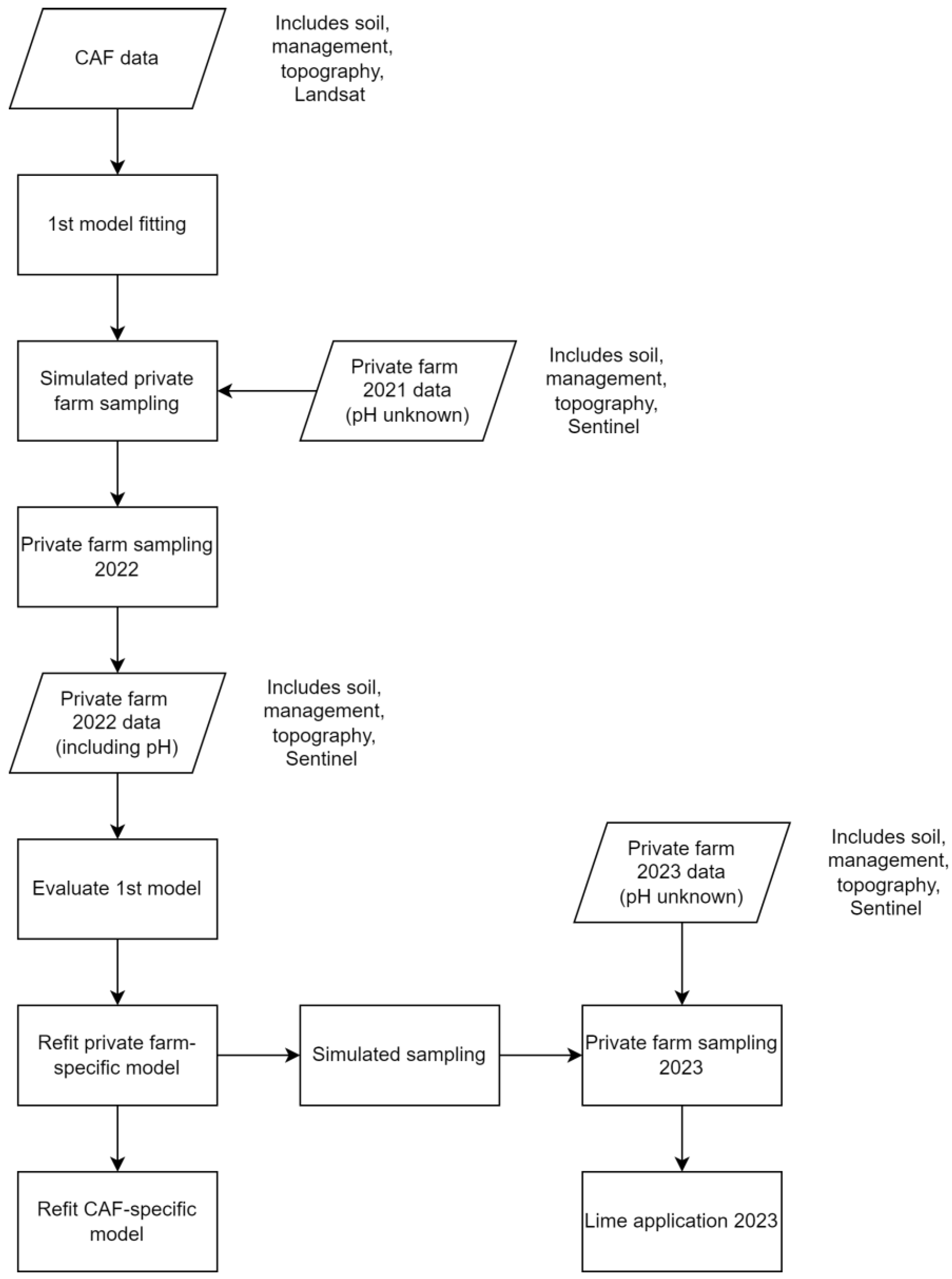
19]. This study combined data from both a long-term research site and a local farm in the Palouse region to develop optimal sampling strategies for the determination of lime requirements in Palouse soils. We first generated a model for soil acidity based on the research site data. Then, we used this model to generate a sampling plan for the local farm and sample accordingly. After evaluating the model’s performance based on soil pH and modified Mehlich buffer tests from the local farm samples, we developed revised models and re-evaluated these at both sites. This method addresses a major problem for farmers in the Palouse, and we expect that sampling plans can be similarly developed to capture field-scale variability in soil acidity on farms throughout the world. With additional test farms, it could be expanded to different regions. A flow chart showing the process used in this study is provided in Figure 1.

2. Methods

The USDA Long-Term Agroecosystem Research (LTAR) region under consideration is shown in Figure 2. The study was conducted on two nearby sites in the Palouse/Eastern WA dryland cropping system: a research farm (the R.J. Cook Agronomy Farm) and a privately owned farm. The Cook Agronomy Farm (CAF) (Figure 3) is a 37 ha site operated as part of the USDA Long-Term Agroecosystem Research (LTAR) network, and a brief description of the vast dataset collected there is included in work by Huggins [20]. Topography is highly variable and has been characterized by a 2 m resolution digital elevation model using a Trimble RTK 4400. Soils are mostly Thatuna (a fine–silty, mixed, superactive, mesic Oxyaquic Argixeroll), Palouse (a fine–silty, mixed, superactive, mesic Pachic Ultic Haploxeroll), and Naff (a fine–silty, mixed, superactive, mesic Typic Argixeroll) soil types [21]. For the on-farm portion, we investigated the northeast quadrant of the property located near Palouse, Washington (Figure 4). Soil survey data indicate that the predominant soil type at this location is Thatuna silt loam [21].
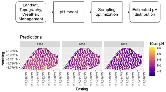
On the CAF, harvest samplings at 369 georeferenced points have been conducted annually for over 20 years of crop rotations. Of these points, 177 were sampled in 1999, 2008, and 2015 with 153 cm deep by 4.1 cm diameter soil cores. Cores were classified, described by soil horizon, and divided into 10 cm depth increments, which were dried, sieved, and analyzed for numerous soil properties, including soil pH (Figure 5 and Figure 6). This was measured in 1:1 soil and water slurries with a Denver Instrument Model 250 pH ISE conductivity benchtop meter or an Accumet AB200 Benchtop pH/Conductivity Meter with a saturated KCl-filled, glass electrode using methods from [6]. Georeferenced points at the CAF farm were additionally sampled for harvested grain and residue biomass in a 2 m2 area. Air- and oven-dried masses of the plant material were measured, and then finely milled sub-samples of grain and residue were analyzed for bulk carbon and nitrogen concentrations via combustion on a Costech ECS4010 Elemental Analyzer. Satellite data consisted of Landsat 5, 7, and 8 analysis-ready multispectral surface reflectance data controlled for clouds, sensor saturation, and other errors, acquired in between the planting and harvest days of harvest years 1999, 2008, and 2015. The following NDVI-based metrics were used in this study: maximum NDVI (NDVI0), maximum rate of NDVI (NDVI1), days after planting when NDVI rate was at a maximum (NDVI2), minimum NDVI (NDVI3), minimum rate of NDVI (NDVI4), and days after planting when NDVI rate was at a minimum (NDVI5).
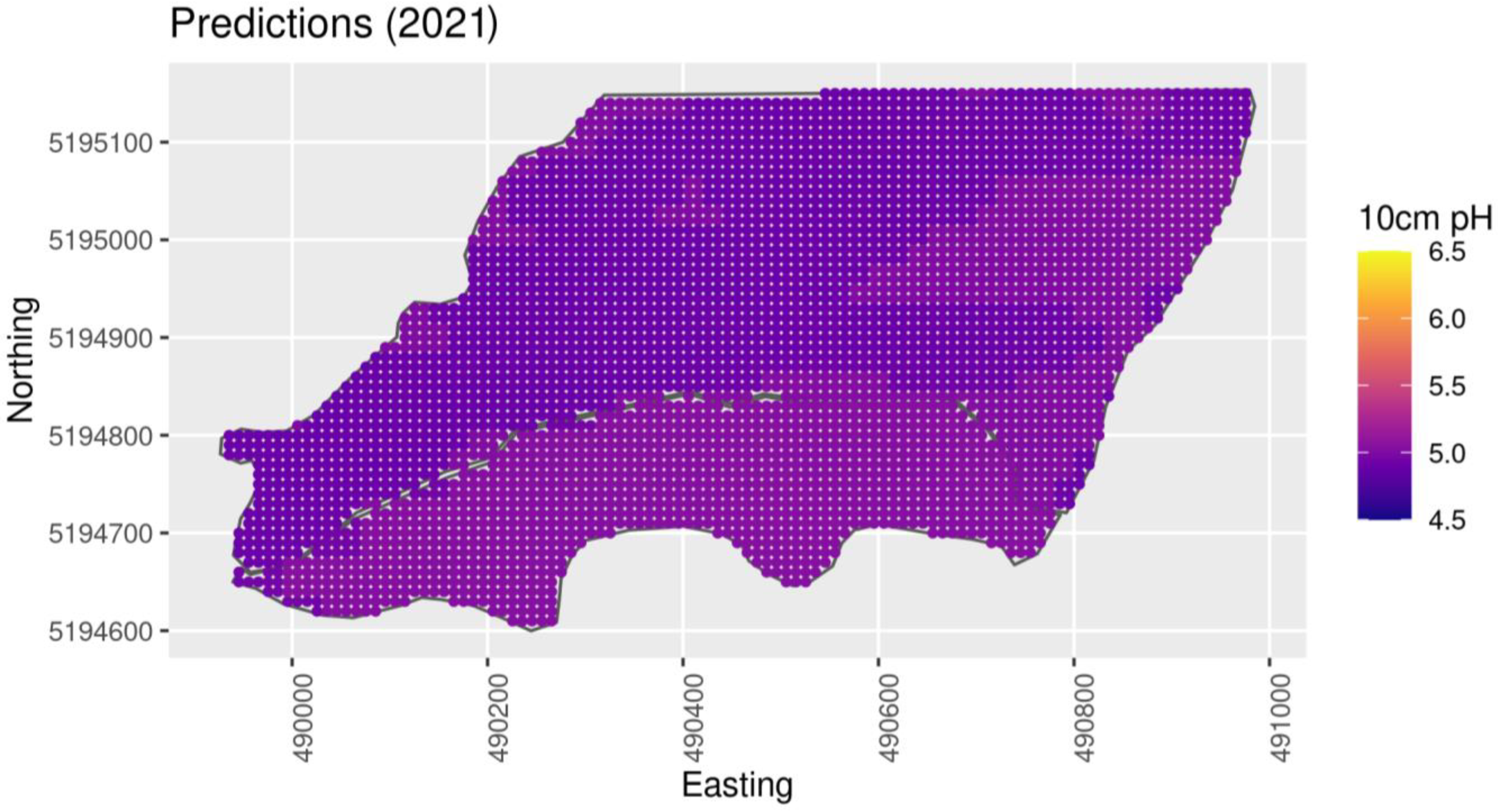
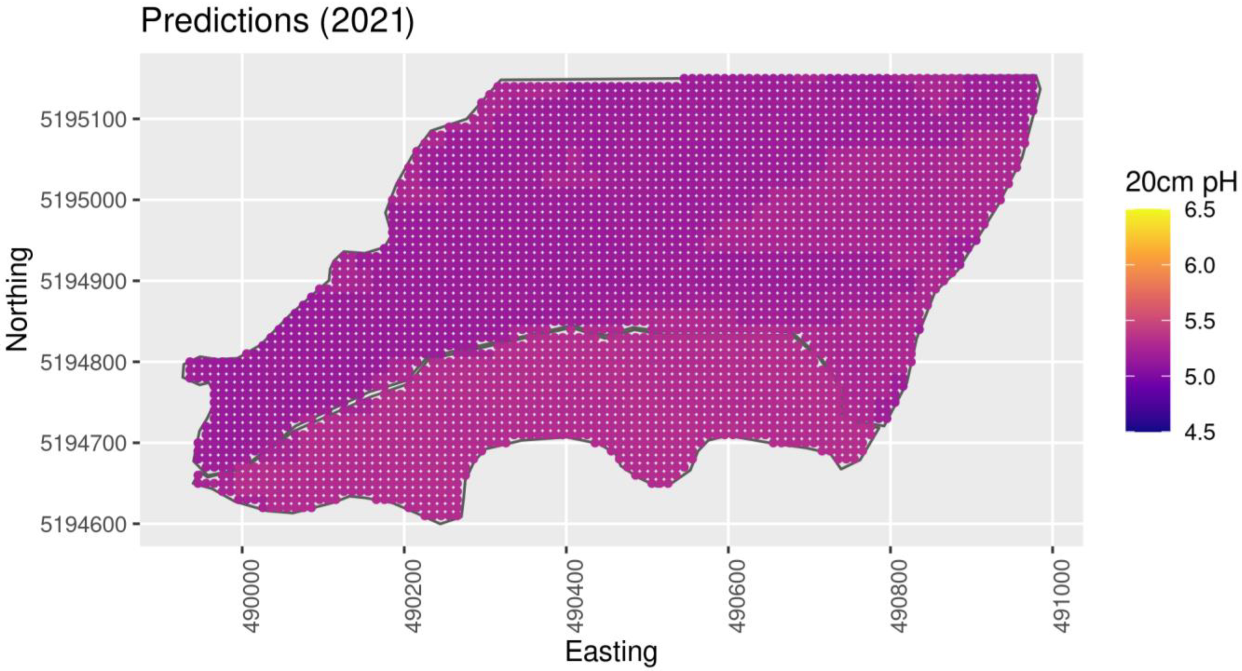
The north section of the private farm, as shown in Figure 4, was planted with chickpeas in 2021; the south was planted in spring with pea. In 2022, the entirety was planted with winter wheat. Following the 2022 wheat harvest, soil sampling occurred at 75 points determined through methods described in subsequent sections. These samples were taken only from 0–10 cm depths due to time and labor constraints, and were analyzed with a Fisher Accumet AB200 probe using similar methods to the CAF sampling procedure given in [22]. Additionally, the farmer specifically requested modified Mehlich buffer pH as an indicator of lime requirements, so this analysis was performed accordingly [23]. Satellite data consisted of Sentinel 2 multispectral data, filtered for cloud cover, acquired in between the planting and harvest days of harvest years 2021 and 2022, and SRTM elevation, all of which we transformed into similar topographical variables as CAF using the same methodology. Multispectral data were also transformed into the same variables as for CAF.
Initial variable selection for the CAF was based on observed correlations in pair plots and known physical relationships (described in Results). A summary of the variables examined in this study is given in Table 1.This was used as the basis for a Bayesian model to generate simulated samplings based on the private farm data for 2021. Modeling for interpolation and simulated sampling was conducted using the spBayes package [16] in R [24]. A multivariate model was chosen to incorporate the strong relationship between pH at 0–10 cm and that at 10–20 cm. The model included exponentially spatially correlated noise as well as a Gaussian sampling error term and covariates derived from management, remote sensing, soil survey, and topography.
Using the spBayes model for CAF to generate synthetic data for the private farm, we developed a k-means stratified random sampling design [10,12]. This design ensures good coverage in space, particular that of relevant covariates. Variables used for cluster generation included face (whether the point was north- or south-facing), GYZ (normalized yield), easting, and northing. Based on typical availability of farm labor, fewer than 100 samples would be practical to collect. In Monte Carlo simulations, 1000 different instantiations of field samplings were generated, each of which was sampled 100 times, for a different number of total samples and k-means clusters (e.g., 100 points and 10 clusters, 80 points and 16 clusters). The means and variogram ranges of soil pH at 0–10 cm and 10–20 cm depths were calculated from the synthetic sampling data for each combination of instance, sampling, sample number, and cluster number. The mean and variance of these soil acidity indicators were calculated for all instances and samplings and compared to values calculated using all points to identify an unbiased sampling design with minimal variance.
Soil samples at 0–10 cm depth were collected at the private farm according to the selected sampling design, and pH and lime requirements were determined as described above. These new data prompted an assessment of the model’s performance. To check the Bayesian model’s interpolation, 20% of the points were withheld, and the root mean squared error (RMSE) and Pearson’s correlation (r) of the interpolated values were used to assess the fit. To cross-validate, this process was repeated 5 times, with different selections for training and testing sets. The Deviance Information Criterion (DIC), also cross-validated, was used to assess the model fit with penalty for parameterization. The CAF model was assessed on the CAF dataset (pH 0–10 cm and pH 10–20 cm) as well as the private farm dataset (pH 0–10 cm only). Cross-validation was not used when testing the 1st CAF model on the private farm, since it was trained on the CAF data.
After initial model assessment, new models were fit for each farm. The CAF dataset did not include modified Mehlich buffer pH, and private farm dataset did not include 10–20 cm soil depths, so separate model structures were necessary for each situation. The final model variable selection was conducted through an exhaustive search for many variables, including the presence of a Bt horizon, NDVI metrics, topographical variables (aspect, slope, and elevation), and nitrogen fertilizer rates. Bt and face were binary indicator variables (i.e., Bt = 0 means no Bt horizon; face = 0 means north-facing). We used dredge from the R package MuMIn [25] with the objective of minimizing the Aikake Information Criterion (AIC). The new models were reassessed as above. Additionally, a qualitative evaluation of the gap filling is provided through the interpolated pH map.

3. Results

3.1. First Model Fitting (CAF)

3.1.1. Model Performance

The first model fitting, using historical data from CAF, included variables (Table 2) that showed a correlation with soil acidity (Figure 7) and that would be available through remote sensing, soil surveys, and management information. This included the aspect (“Face”, north- or south-facing). We also added yield normalized over the field (GYZ), which was gap-filled with a second model based on the maximum NDVI achieved during the growing season. This simplified model performed poorly, with an RMSE of 0.3871446 for interpolation of soil pH at 0–10 cm of depth, and of 0.37456 for soil pH at 0–20 cm of depth (Table 3) and Pearson’s correlation of −0.1129 and 0.3015 for the two depths (Table 4). The DIC (Table 5) was −721.7108, a reasonable value given the large field-scale variability in soil pH and the purpose of the initial model. As we lacked pH data from the private farm, it was better to have a more general model to design the initial sampling scheme.

3.1.2. Sampling Design

After generating thousands of simulated sampling experiments with the Bayesian model with inputs from the private farm in harvest year 2021, we examined the mean and variance of sample estimates of global mean soil pH at 0–10 cm of depth and the variogram range parameter of pH at 0–10 cm, as well as the same variables for pH at 10–20 cm. Figure 8 and Figure 9 show one simulated pH distribution generated during simulated sampling. From the Supplementary Material, in Figures S1 and S2, we see that in general, there was a very small bias in mean pH regardless of the sample number and number of clusters, and sample variance tended to decrease with increasing sample number. For the semivariogram range (Figures S3 and S4), which was more affected by the spatial distribution of the samples, the trends were less consistent, but simulated samplings with 50–100 samples and 10–18 clusters showed lower bias and lower variance estimates for pH at 0–10 cm. The bias was higher for 10–20 cm, as the true range for this depth is larger and is thus more strongly affected by sample spatial distribution. Based on these results, we chose 15 k-means centers with 75 total points as a good compromise between accuracy for pH at 0–10 cm and available farm labor.

3.1.3. CAF Model Performance on Private Farm

Figure 10 and Figure 11 show the pH measured at 0–10 cm and the modified Mehlich buffer pH (MMpH), which was measured at the farmer’s request. Deeper sampling was impractical due to the dry conditions during the window of time available for soil sampling on the farm. One feature evident in the data was higher pH values near field boundaries, but other trends were not clearly discernible. The first CAF model performed poorly on the subsequent pH measurements from the on-farm samples, with an RMSE of 0.3084. This indicated that reassessment of the original model was necessary.

3.2. Second Model Fitting (CAF and Private Farm)

After fitting a new model with the on-farm soil pH data, we found new remote sensing correlates with pH, NDVI2, and NDVI5, with NDVI5 having a stronger relationship. NDVI2 and NDVI5 represent the days after planting of peak greening rate and peak senescence rate, respectively. These slopes were positive, indicating that areas with earlier senescence were more likely to have a low pH. Additional covariates were terrain slope and the presence of a Bt horizon. The negative coefficient of the terrain slope term implies flatter areas such as ridges were more likely to have a higher pH, perhaps due to exposure of basic subsoil layers by erosion. Areas with Bt horizons had a lower pH. When the new model was used for Bayesian interpolation (Figure 12 and Figure 13), the RMSE was lower than with the original CAF model at 0.2487 for soil pH at 0–10 cm and 0.1221 for MMpH at 0–10 cm, with a Pearson’s r of 0.3653 and 0.3094.
Similarly, when CAF was reassessed with the updated model, we found relationships with NDVI5, Bt, terrain slope, and aspect (face). NDVI0 and NDVI4 (maximum NDVI and peak senescence rate) also correlated with soil pH. In contrast to the private farm, pH was higher for samples from south-facing areas and regions with Bt horizons. The new model shows an improved RMSE of interpolation of 0.3272 for 0–10 cm and 0.3381 for 10–20 cm, with a Pearson’s r of 0.2682 and 0.2283, and the DIC was −1551.0380, being higher than that of the initial model due to the increased number of parameters.

4. Discussion

The CAF long-term agricultural research site provided a rich historical dataset, permitting the development of a model for interpolation of soil pH from limited direct measurements based on factors that could be easily measured in on-farm settings. The private farm in turn provided a complementary dataset at a similar commercial site, permitting the improvement in model performance on both the CAF and the private farm. The farmer will use the data collected in a follow-up sampling in 2023 based on the improved model to make real-world decisions regarding lime application to raise soil pH with minimal input waste and soil testing costs to accommodate practical constraints surrounding farm labor and timing of farm operations. Having established a working relationship with a farmer, we can continue sampling in subsequent seasons to observe the outcomes of a precision agriculture approach in a real-world scenario that would not be feasible on the research farm. The drawbacks of the on-farm approach were primarily the constraints imposed by working around the field operations and the limited availability of historical data for the farm. This approach combining long-term and on-farm research demonstrates the power of researcher–stakeholder collaborations and knowledge co-production in agriculture [17].
A few interesting trends were observed in the data when both farms were considered. NDVI5, slope, and Bt horizons were important covariates on both farms. This shows that senescence timing, topography, and restrictive layers such as argillic horizons all influence the field-scale variability of soil pH. Early senescence was associated with low soil pH on both farms. This could represent a soil-acidifying feedback loop whereby limited crop growth results in decreased evapotranspiration to counteract the downward leaching of base cations through the soil profile [2], decreased nitrogen uptake results in further soil acidification via nitrification of excess ammoniacal fertilizer, and soil-acidity-induced Al toxicity results in an ongoing decrease in crop growth [2]. However, the senescence rate must be used with care to predict soil pH as some crops, such as chickpeas, are chemically senesced for harvest. The two farms exhibited opposing trends linking soil pH to the presence of Bt horizons, possibly reflecting differences in the continuities and spatial extents of the restrictive layers. The link between low soil pH and Bt horizons on the private farm could be explained by localized decreased rooting depth leading to decreased evapotranspiration and decreased nitrogen uptake, similarly to early senescence. On the other hand, the link between high soil pH and Bt horizons on the CAF research site could reflect argillic horizons with sufficient continuity and spatial extent to create seasonally perched water tables that limit the downward leaching of base cations and lead to high soil moisture levels that inhibit microbial nitrification reactions. Regardless of the mechanisms, senescence timing, topography, and Bt horizons (via soil survey data) are all simpler to assess than soil pH in on-farm settings such that the model developed from the CAF and private farms can be used to improve the efficiency of lime applications without burdensome soil testing.
The interpolation results show satisfactorily low RMSEs could be obtained for pH and MMpH at 0–10 cm, using a limited number of samples, in comparison to other studies predicting pH, which achieved RMSEs of 0.3–0.35 [7,8]. The DIC of the initial model versus that of the revised models shows that increasing the number of parameters improved the applicability of this technique for designing precision lime applications, where fine-resolution maps of buffer pH are needed but difficult to obtain for farms over 50 ha. However, some sampling is still necessary to capture the baseline level of acidity. This depends a great deal on the long-term management history, which can be difficult to incorporate into a model.

5. Conclusions

The acidifying agricultural landscape of the inland Pacific Northwest requires remediation of soil if farms are to remain productive. One amendment, lime, can be applied, but its high expense means that precision application is necessary. This requires high-resolution soil sampling, which is another expense. This paper developed a methodology using remote sensing and soil survey variables to optimize sampling and increase interpolation accuracy through Bayesian modeling and synthetic sampling experiments. We showed the potential of the technique by testing the method on a farmer’s property. In doing so, we were able to improve our initial model. Future work will include yearly sampling campaigns on both the privately owned farm and our research farm, including generating prescription maps for lime. Further work is needed on additional farms in different regions to test whether it can be extended to different soil types and cropping systems, and to determine if there are generalized limits on the number of samples or resolution required.

Supplementary Materials

The following supporting information can be downloaded at: https://www.mdpi.com/article/10.3390/rs15123105/s1, Figure S1: Global mean pH estimated by sample mean in simulated sampling experiments, compared with population value estimated from CAF model; Figure S2: Sample variance of global mean in simulated sampling experiments; Figure S3: Semivariogram range estimated by sample mean in simulated sampling experiments, compared with population value estimated from CAF model; Figure S4: Sample variance of semivariogram range in simulated sampling experiments.

Author Contributions

Conceptualization, J.J.C.; Data curation, J.J.C.; Formal analysis, J.J.C.; Methodology, J.J.C. and J.L.C.; Writing—review and editing, M.L. All authors have read and agreed to the published version of the manuscript.

Funding

This research received no external funding.

Data Availability Statement

Data for CAF are available on request (though cafltar.org, accessed on 3 March 2023). Data from the private farm are subject to a cooperative agreement and may need additional information from requesters. Contact the lead author for inquiries.

Acknowledgments

This research was a contribution from the Long-Term Agroecosystem Research (LTAR) network. LTAR is supported by the United States Department of Agriculture. This research used resources provided by the SCINet project of the USDA Agricultural Research Service, ARS project number 0500-00093-001-00-D. The authors would also like to thank Anali Osorio for her help in pH testing.

Conflicts of Interest

The authors declare no conflict of interest.

References

  1. Brown, T.; Koenig, R.T.; Harsh, J.B.; Huggins, D.R.; Rossi, R.E. Stratified Soil Acidity and the Potential for Aluminum Toxicity in Inland Pacific Northwest Direct-Seed Cropping Systems. In Proceedings of the ASA-CSSA-SSSA International Meetings, Salt Lake City, UT, USA, 6–10 November 2005. [Google Scholar]
  2. Slessarev, E.W.; Lin, Y.; Bingham, N.L.; Johnson, J.E.; Dai, Y.; Schimel, J.P.; Chadwick, O.A. Water balance creates a threshold in soil pH at the global scale. Nature 2016, 540, 567–569. [Google Scholar] [CrossRef] [PubMed] [Green Version]
  3. Bezdicek, D.F.; Beaver, T.; Granatstein, D. Subsoil ridge tillage and lime effects on soil microbial activity, soil pH, erosion, and wheat and pea yield in the Pacific Northwest, USA. Soil Tillage Res. 2003, 74, 55–63. [Google Scholar] [CrossRef]
  4. Peng, Q.; Huggins, D.R. No-till farming for managing soil organic matter in semiarid, temperate regions: Synergies, tradeoffs, and knowledge gaps. In Soil Organic Matter and Feeding the Future; Lai, R., Ed.; CRC Press: Boca Raton, FL, USA, 2021; pp. 365–406. ISBN 9780367609702. [Google Scholar]
  5. McFarland, C.; Shiwakoti, S.; Carpenter-Boggs, L.; Schroeder, K.; Brown, T.; Huggins, D.R. Evaluating buffer methods for deter-mining lime requirement on acidified agricultural soils of the Palouse. Soil Sci. Soc. Am. J. 2020, 84, 1769–1781. [Google Scholar] [CrossRef]
  6. McFarland, C. Liming No-Till Soils and Determining Lime Requirement in the Palouse Region. Ph.D. Thesis, Washington State University, St. Pullman, WA, USA, 2016. [Google Scholar]
  7. Gogumalla, P.; Rupavatharam, S.; Datta, A.; Khopade, R.; Choudhari, P.; Dhulipala, R.; Dixit, S. Detecting Soil pH from Open-Source Remote Sensing Data: A Case Study of Angul and Balangir Districts, Odisha State. J. Indian Soc. Remote Sens. 2022, 50, 1275–1290. [Google Scholar] [CrossRef]
  8. Zhang, Y.; Sui, B.S.; Shen, H.; Wang, Z. Estimating temporal changes in soil pH in the black soil region of Northeast China using remote sensing. Comput. Electron. Agric. 2018, 154, 204–212. [Google Scholar] [CrossRef]
  9. Brus, D.J.; De Gruijter, J.J. Random sampling or geostatistical modelling? Choosing between design-based and model-based sam-pling strategies for soil (with discussion). Geoderma 1997, 80, 1–44. [Google Scholar] [CrossRef]
  10. Brus, D.J.; Heuvelink, G.B. Optimization of sample patterns for universal kriging of environmental variables. Geoderma 2007, 138, 86–95. [Google Scholar] [CrossRef]
  11. Wang, W.; Zhao, Y.; Zhang, T.; Wang, R.; Wei, Z.; Sun, Q.; Wu, J. Regional soil thickness mapping based on stratified sampling of optimally selected covariates. Geoderma 2021, 400, 115092. [Google Scholar] [CrossRef]
  12. Kidd, D.; Malone, B.; McBratney, A.; Minasny, B.; Webb, M. Operational sampling challenges to digital soil mapping in Tasmania, Australia. Geoderma Reg. 2015, 4, 1–10. [Google Scholar] [CrossRef]
  13. Wikle, C.K.; Zammit-Mangion, A.; Cressie, N. Spatio-Temporal Statistics with R; Chapman and Hall/CRC: Boca Raton, FL, USA, 2019; ISBN 9780429649783. [Google Scholar]
  14. Ozaki, V.A.; Ghosh, S.K.; Goodwin, B.K.; Shirota, R. Spatio-Temporal Modeling of Agricultural Yield Data with an Application to Pricing Crop Insurance Contracts. Am. J. Agric. Econ. 2008, 90, 951–961. [Google Scholar] [CrossRef] [PubMed] [Green Version]
  15. Wikle, C.K.; Hooten, M.B. A general science-based framework for dynamical spatio-temporal models. Test 2010, 19, 417–451. [Google Scholar] [CrossRef]
  16. Finley, A.; Banerjee, S.; Carlin, B. spBayes: An R Package for Univariate and Multivariate Hierarchical Point-Referenced Spatial Models. J. Stat. Softw. 2007, 19, 1–24. [Google Scholar] [CrossRef] [PubMed] [Green Version]
  17. Kleinman, P.; Spiegal, S.; Rigby, J.; Goslee, S.; Baker, J.; Bestelmeyer, B.; Boughton, R.; Bryant, R.; Cavigelli, M.; Derner, J.; et al. Advancing the sustainability of US agriculture through long-term research. J. Environ. Qual. 2018, 47, 1412–1425. [Google Scholar] [CrossRef] [PubMed]
  18. Lacoste, M.; Cook, S.; McNee, M.; Gale, D.; Ingram, J.; Bellon-Maurel, V.; MacMillan, T.; Sylvester-Bradley, R.; Kindred, D.; Bramley, R.; et al. On-Farm Experimentation to transform global agriculture. Nat. Food 2022, 3, 11–18. [Google Scholar] [CrossRef] [PubMed]
  19. Piepho, H.-P.; Richter, C.; Spilke, J.; Hartung, K.; Kunick, A.; Thöle, H. Statistical aspects of on-farm experimentation. Crop Pasture Sci. 2011, 69, 721–735. [Google Scholar] [CrossRef]
  20. Huggins, D.R. The Cook Agronomy Farm LTAR: Knowledge Intensive Precision Agro-ecology. In Proceedings of the AGU Fall Meeting, San Francisco, CA, USA, 14–18 December 2015. [Google Scholar]
  21. NRCS Whitman County, WA Soil Survey. Available online: http://websoilsurvey.sc.egov.usda.gov/App/HomePage.htm (accessed on 3 March 2023).
  22. McFarland, C.; Huggins, D.R. Acidification in the inland Pacific Northwest. Crops Soils 2015, 48, 4–12. [Google Scholar] [CrossRef]
  23. Hoskins, B.R.; Erich, M.S. Modification of the Mehlich lime buffer test. Commun. Soil Sci. Plant Anal. 2008, 39, 2270–2281. [Google Scholar] [CrossRef]
  24. R Core Team. R: A Language and Environment for Statistical Computing; R Foundation for Statistical Computing; R Core Team: Vienna, Austria, 2013. [Google Scholar]
  25. Barton, K. MuMIn: Multi-Model Inference. Available online: http://r-forge.r-project.org/projects/mumin (accessed on 10 October 2022).
Figure 1. Flow chart illustrating the model development and sampling process.
Remotesensing 15 03105 g001
Figure 2. Map showing the research region. The blue star indicates the location of the R.J. Cook Agronomy Farm.
Remotesensing 15 03105 g002
Figure 3. R.J. Cook Agronomy Farm, east field (46°47′N, 117°5′W) northeast of Pullman, WA, RapidEye-4 surface reflectance, 7 August 2015. This area represents a 37 ha field and is a site for long-term agroecological research. Soil sampling locations are indicated by black dots.
Remotesensing 15 03105 g003
Figure 4. Map of farmer’s field under study. Soil sampling locations are indicated by black dots.
Remotesensing 15 03105 g004
Figure 5. Cook Agronomy Farm observations of soil pH at 0–10 cm of depth.
Remotesensing 15 03105 g005
Figure 6. Cook Agronomy Farm observations of soil pH at 10–20 cm of depth.
Remotesensing 15 03105 g006
Figure 7. Observed correlations with soil pH from CAF data. Since face is a categorical variable, no correlation is given, and it is instead plotted as a boxplot and as histograms of pH for each face value (north and south). GYZ represents normalized yield and is dimensionless. *** indicates significance at 0.001 and ** at 0.01.
Remotesensing 15 03105 g007
Figure 8. CAF model prediction of soil pH at 0–10 cm on the private farm.
Remotesensing 15 03105 g008
Figure 9. CAF model prediction of soil pH at 10–20 cm on the private farm.
Remotesensing 15 03105 g009
Figure 10. Observations of soil pH at 0–10 cm on a private farm.
Remotesensing 15 03105 g010
Figure 11. Observations of modified Mehlich buffer pH at 0–10 cm on a private farm.
Remotesensing 15 03105 g011
Figure 12. Model prediction of soil pH at 0–10 cm on the private farm.
Remotesensing 15 03105 g012
Figure 13. Model prediction of modified Mehlich buffer pH at 0–10 cm on the private farm.
Remotesensing 15 03105 g013
Table 1. Summary of variables examined in this study.
TypeVariables
CropCrop (crop type), GrainYield (dry grain per area), GYZ (GrainYield, Z-normalized)
ManagementNf, Kf, Pf (applied nitrogen, phosphorous, and potassium per area)
TopographyAspect, TRASP (transformed aspect), Face, Elevation, Slope, AnalyticalHillshade, TopographicalWetnessIndex, ConvergenceIndex
MeteorologyTave (season average daily temperature), Precip (total precip in calendar year before harvest)
SoilpH10 (0–10 cm pH), pH20 (10–20 cm pH), MMpH10 (0–10 cm Modified Mehlich pH), Bt (presence of argillic horizon)
Remote sensingNDVI0 (maximum Normalized Difference Vegetation Index), NDVI1 (maximum NDVI rate), NDVI2 (days after planting of maximum NDVI rate), NDVI3 (minimum NDVI), NDVI4 (minimum NDVI rate), NDVI5 (days after planting of minimum NDVI rate)
Table 2. pH model equations and adjusted R2 of the fit, with p-values, used within this paper.
ModelEquationR2 (p)
CAF (1st model) pH10 = Face + GYZ
pH20 = Face + GYZ
GYZ = Bt + Precip + Tave + Crop * (NDVI0 + Face)
0.03663 (0.001447)
0.04093 (0.0007449)
0.06222 (<2.2 × 10⁻¹⁶)
Private farmpH10 = Bt + NDVI2 + NDVI5 + Slope
MMpH10 = NDVI2 + NDVI5
0.1345 (0.006699)
0.1808 (0.0002844)
CAF (2nd model)pH10 = Bt + Elevation + Face + NDVI4 + NDVI5
pH20 = Bt + Elevation + Face + NDVI0 + NDVI5 + Slope
0.09525 (2.375 × 10⁻¹¹)
0.06468 (2.05 × 10⁻⁷)
Table 3. pH model performance with 5-fold cross-validated RMSE.
ModelData for EvaluationRMSE 0–10 cm pHRMSE 10–20 cm pHRMSE 0–10 cm MM pH
CAF (1st model)CAF0.38710.3746NA
CAF (1st model)Private farm 20220.3084NANA
Private farmPrivate farm 20220.2487NA0.1221
CAF (2nd model)CAF0.32720.3381NA
Table 4. pH model performance with 5-fold cross-validated Pearson’s correlation coefficient.
ModelData for Evaluationr 0–10 cm pHr 10–20 cm pHr 0–10 cm MM pH
CAF (1st model)CAF−0.11290.3015NA
CAF (1st model)Private farm 20220.0726NANA
Private farmPrivate farm 20220.3653NA0.3094
CAF (2nd model)CAF0.26820.2283NA
Table 5. pH model performance with 5-fold cross-validated DIC.
ModelData for EvaluationDIC of Bayesian Model
CAF (1st model)CAF−721.7108
Private farmPrivate farm 2022−382.8158
CAF (2nd model)CAF−1551.0380
Disclaimer/Publisher’s Note: The statements, opinions and data contained in all publications are solely those of the individual author(s) and contributor(s) and not of MDPI and/or the editor(s). MDPI and/or the editor(s) disclaim responsibility for any injury to people or property resulting from any ideas, methods, instructions or products referred to in the content.

