Article

Oceanic Responses to the Winter Storm Outbreak of February 2021 in the Gulf of Mexico from In Situ and Satellite Observations

1
NOAA’s National Centers for Environmental Information (NCEI), Silver Spring, MD 20910, USA
2
Earth System Science Interdisciplinary Center (ESSIC), Cooperative Institute for Satellite Earth System Studies (CISESS), University of Maryland, College Park, MD 20740, USA
3
Northern Gulf Institute, Mississippi State University, Stennis Space Center, MS 39529, USA
4
NOAA’s National Centers for Environmental Information, Stennis Space Center, MS 39529, USA
5
NOAA’s National Centers for Environmental Information, Asheville, NC 28801, USA
*
Author to whom correspondence should be addressed.
Remote Sens. 2023, 15(12), 2967; https://doi.org/10.3390/rs15122967
Submission received: 15 April 2023 / Revised: 25 May 2023 / Accepted: 3 June 2023 / Published: 7 June 2023

Abstract

:
Winter storms occur in the Gulf of Mexico (GoM) every few years, but there are not many studies on oceanic responses to severe winter storms. Although usually considered less destructive than hurricanes, they can result in cumulative damages. Winter Storm Outbreak of February 2021 (WSO21), the most intense winter storm to impact Texas and the GoM in 30 years, passed over the western GoM and brought severe cold to the GoM coastal regions, which caused a sudden cooling of the ocean surface, resulting in an extensive loss of marine life. In this study, we analyze multiple datasets from both in situ and satellite observations to examine the oceanic changes due to WSO21 in order to improve our understanding of oceanic responses to winter storms. Although the pre-storm sea surface temperature (SST) was 1–2 °C warmer than normal, severe coastal cold spells caused a significant cooling of the order of −3 °C to −5 °C during WSO21 and a −1 °C average cooling in the mixed layer (ML) over the western GoM. Net surface heat loss played a primary role in the upper ocean cooling during WSO21 and explained more than 50% of the cooling that occurred. Convective mixing due to surface cooling and turbulent mixing induced by enhanced wind speeds significantly increase the surface ML in the western GoM. Apart from rapid changes in SST and heat fluxes due to air-sea interactions, persistent upwelling brings nutrients to the surface and can produce coastal “winter” blooms along the Texas and Mexico coast. Prominent salinity increases along the coastal regions during and after WSO21 were another indicator of wind-induced coastal upwelling. Our study demonstrates the utility of publicly-available datasets for studying the impact of winter storms on the ocean surface.

1. Introduction

Despite the rapid warming of the global atmosphere and ocean, the United States (U.S.) has experienced an increasingly frequent number of extremely cold winter weather events over the past several decades [1]. The occurrences of many winter storms (also known as cold waves/fronts/snaps) in the U.S. are associated with the frequency of polar stretched vortexes [1]. Winter storm-induced cooling and mixing is one of the main causes of marine cold spells (MCSs) in the U.S. coastal regions. A marine cold spell is a period of exceptionally cold surface water that has an acute impact on the marine ecosystem [2].
The first United States billion-dollar weather-related disaster in 2021 was from a winter storm. This storm has been commonly referred to as the “Great Texas Freeze”, “Winter Storm Uri”, or, the term used in this study, “Winter Storm Outbreak of February 2021 (WSO21)”. Unlike many other winter storms (e.g., the blizzard of 1996), where snow and other forms of frozen precipitation made the headlines, WSO21 is most infamous for the severe and long-lasting cold it brought to the south-central and Gulf Coast of the United States and, in particular, Texas and the northwest Gulf of Mexico (GoM). WSO21 caused cascading failures of natural gas supplies, power generation and interconnected energy systems in Texas, which restricted the electricity supply and left more than 4.5 million Texans without heat or electricity for several days [3]. In Texas, at least 246 individuals died directly or indirectly due to the severe cold [4]. The total damages were estimated to amount to approximately USD 295.0 billion [5].
WSO21 came about due to disruptions in the synoptic-scale atmospheric pattern in mid-February 2021. The polar vortex was in a weakened state and the Arctic Oscillation was in a strongly negative phase; this allowed for a large and deep trough to develop over central United States which funneled Arctic air southward from Canada to Texas. WSO21 was associated with three separate cold fronts that came through southeastern Texas between 2/11 and 2/17 and helped pump cold air into the region: a weaker front on 2/11 and a much stronger front on 2/14, followed by a weaker front on 2/17. It was also reported using the National Weather Service’s Weather Prediction Center (WPC) surface analysis of pressure fields and upper air patterns (500 hPa height contours) that the cold arctic air gradually spilled southward into Texas, resulting in precipitation in the form of snow, sleet and freezing rain. The WPC surface analysis showed the three prominent cold fronts passing through the GoM over the same period (https://www.weather.gov/fwd/Feb-2021-WinterEvent) (accessed on 17 May 2023). The Arctic cold front that pushed through on 2/14 shattered many cold temperature records throughout the state of Texas. It was the coldest winter storm experienced in this area since December 1989. Galveston, which is located on the southeast coast of Texas and where the temperature is often modulated by the GoM, experienced 37 consecutive hours of below-freezing temperatures from 2/15 to 2/16. Additionally, their daily average temperature departure from normal was −10.8 °C between 2/12 and 2/18, with a −16.7 °C departure experienced on 2/15.
WSO21 was a very dynamic and complex weather system, but satellite and weather stations allow for attempts to understand the different atmospheric processes and their effect on land [3,6]. However, due to the lack of studies on the ocean, the oceanic processes during winter storms are still not well understood.
Winter storms can occur every few years in the GoM [7], with severe events recorded in 1899, 1940, 1951, 1983, 1989, 2011 and 2021 [3,8]. The GoM has a long coastline with a large body of shallow bay water. Because the coastal water is so shallow, winter storms can cause dramatic drops in coastal water temperature accompanied by extremely rapid air temperature drops. Besides impacts on human and land ecological systems, winter storms also influence ecosystems in the GoM. Significant marine life mortality and extensive destruction have occasionally been observed in the coastal region (e.g., [8,9,10,11]) after a winter storm passage. For example, at least 1 million pounds of fish perished due to cold in the bay water of the GoM during the January 1940 MCS [8], and 60–90 million pounds of fish perished during the 1951 MCS [9]. Three MCSs that occurred in the Texas coastal region in the 1980s caused the death of ~32 million fish in total [11]. Both the duration of the MCS and the rapidity of the temperature drop played important roles in influencing the amount of fish mortality [8,9]. The damage to fish caused by an MCS event can bring a significant reduction to the commercial catch in the following year [8,9]. Cold weather events in the GoM can cause sea turtle cold-stun stranding events (e.g., thousands of juvenile green sea turtles were stranded in St. Joseph Bay, Florida, in the winter of 2010 [12]). During WSO21, more than 12,000 cold-stunned sea turtles were rescued along the Texas coast, and only 35% of them survived, making it the largest sea turtle cold-stun event in recorded history [13]. At least 3.8 million fish were killed coastal-wide due to WSO21, the highest fish mortality rate in the past 30 years [11]. WSO21 also influenced coastal wetlands and caused ecosystem shifts between salt marshes and mangroves along the Texas coast [14].
Winter storms over the GoM can cause accelerated oceanic heat loss and sea surface temperature (SST) decreases through wind-driven upwelling and convective mixing [15,16,17]. The GoM SST has a clear seasonal cycle, with the minimum SST typically occurring in February or March (13–15 °C in the northern coastal regions [18,19], 22–24 °C in the western gulf and 24–26 °C in the eastern gulf [15]). The Gulf of Mexico Regional Climatology [20], generated from historical ocean profile data within the World Ocean Database [21], estimated the long-term mean conditions over the 1955–2017 period. The long-term mean conditions during February are shown in Figure 1. Figure 1a displays the February SST climatology, with the coldest waters (<16 °C) along the United States coast in the northwest GoM, with a gradual increase in temperature with decreasing latitude, reaching temperatures >26 °C in the Yucatán Basin. To understand the background vertical structure from climatology, a 0–200 m meridional cross-section at 95°W (Figure 1b) and 0–200 m zonal cross-section at 28°N (Figure 1c) in the GoM is plotted. Figure 1b reveals fresh (salinity < 34) and cold (<15 °C) water near the northwest coast, which rapidly increases towards the south, and Figure 1c shows rapidly increasing temperature and salinity from near the Texas coast to the interior Gulf. Thus, the expected climatological conditions near the northwest coast of GoM (Texas) are for the near-coast to experience fresh (<34) and cold (<15 °C) conditions with rapidly increasing temperature and salinity towards the interior Gulf. Based on Figure 1b,c, temperatures are vertically homogeneous throughout much of the GoM, with increasing vertical stratification occurring at approximately 100 m in the interior GoM, driven by rapidly decreasing temperatures at this depth. Salinity is vertically uniform in the mixed layer (ML), but increases slightly to >36.4 below the ML and then decreases again with depth.
More winter storms could occur during the El Niño–Southern Oscillation years and could cause enhanced mixing of the upper water column, which might result in higher phytoplankton concentrations in the deep GoM [16]. Muller-Karger et al. [22] found that cooler winters relative to the seasonal climatology were less frequent in the 2000s than in the 1980s in the GoM, which was likely due to global warming. A winter storm could cause periodic upwelling and the offshore transport of nutrient-rich water from the coast to the inner shelf of the northern GoM, resulting in enhanced phytoplankton growth in the inner shelf regions [23]. Winter storms are also critical in determining the long-term sediment-transport pathways in the northern GoM [24].
Although winter storms can cause billions of dollars in losses and massive ecosystem damages that are comparable to those resulting from tropical storms and hurricanes, their oceanic responses have not received sufficient attention to date. In this study, we combined available data from both in situ and remote satellite observations to characterize the oceanic changes during WSO21 in the GoM. The focus will be specifically on the cooling process because that was one of the most notable phenomena that occurred during this winter storm. A physical understanding of how the upper ocean responds to a winter storm may be useful for conservation, management and modeling purposes. We also discuss how MCS changes with time under a regime of global warming and climate change as winter storms are one of the biggest contributors to MCS. The frequency and intensity of MCS are decreasing globally due to SST warming [25]. The average SST over the GoM has risen at a rate of approximately 0.15–0.3 °C/decade since the 1980s [18,22,26,27] and, during the most recent decades (2011–2022), the average SST has increased by >1.0 °C compared to that in the 1970s [27]. We use WSO21, one of the most recent and intense winter storms, to investigate how the GoM responded to a severe winter weather event. We investigate changes in SST, turbulent heat fluxes, salinity, wind, chlorophyll-a, mixed layer depth (MLD) and upwelling, with a special focus on the mechanisms controlling the water temperature cooling process during WSO21.
The structure of this paper is as follows. The Section 2 describes datasets and analysis methods. The Section 3 describes the results, followed by a discussion in Section 4 and a summary of this study in Section 5.

2. Data and Methods

To improve our understanding of how the surface ocean responded to WSO21, we consider both in situ and satellite observations collected in February 2021. We analyze SST anomalies derived from removing the long-term climatological mean and also review the before, during and after storm conditions caused by WSO21 for multiple other geophysical and biological variables discussed in this section. The primary focus of this study is the western GoM (west of 90°W; white rectangle in Figure 2).

2.1. Datasets

2.1.1. Surface Buoy Observations

Surface buoy data were obtained from the National Buoy Data Center (NBDC) and Texas Automated Buoy System (TABS) in the western GoM. Buoy locations with bathymetry data are shown in Figure 2a and Table 1. Only buoys with SST observations in February 2021 were selected for our analysis. There was a total of 10 stations that met this criterion (Table 1). Most buoys also measure air temperature, wind speed and direction, and sea level pressure. Salinity (density) and water current speed/direction observations were all obtained from the TABS. For wind and current directions, we followed the nautical definition. The direction of the wind was considered as the direction from where it was blowing, while the direction of ocean currents was considered as the direction they were headed for. Buoy names are shown next to the buoy stations (red squares) in Figure 2a. Stations PTAT2 and ANPT2 are so close to each other that they cannot be shown separately. Stations 42043, 42045 and 42048 are TABS buoys and, therefore, have both five-digital NDBC buoy names and one-letter TABS buoy names, with the TABS name shown in parenthesis. Buoy X is a TABS buoy with no NBDC name. The listing order of stations in Table 1 is based on their water depths from shallow to deep, roughly corresponding to the distance offshore. The shallowest station is PTAT2, with water depth observations of 1.0 m, while the deepest station (42002) is located at more than 3000 m. For stations with two names in Table 1, the one in parenthesis is the TABS name. For the variable changes due to WSO21, the mean shows the average difference between Periods III and I (the average between 13–21 February 2021 minus the average between 8–10 February 2021). The max shows the maximum/minimum changes due to WSO21 (the minimum is shown for air and water temperatures and the maximum is shown for the rest of the variables). A blank space in Table 1 means the variable was not measured at that station.

2.1.2. Daily Optimum Interpolation Sea Surface Temperature (DOISST)

SST and SST Anomaly (SSTA) data were derived from the National Oceanic and Atmospheric Administration (NOAA) DOISST version v2.1, which is a global daily SST product with a spatial resolution of 0.25°, starting from September 1981 [28,29]. DOISST blends in situ and bias-corrected advanced very high-resolution radiometer (AVHRR) SST measurements. The AVHRR SSTs were adjusted to the global buoy SSTs at the nominal depth of 0.2 m. In the ice-covered regions, the proxy SSTs from ice concentrations [30] were blended with other in situ and AVHRR SSTs, if available. Figure 2b shows the SST map obtained from the DOISST during the pre-storm period (the average between 8 and 10 February 2021) as an example.

2.1.3. Wind and Surface Heat Flux Data

The new version of a blended wind product (NOAA NCEI Blended Seawinds version v2.0-NBSv2) [31], which was developed recently to resolve very high winds associated with hurricanes and storms, was used to determine the Ekman suction/pumping from the curl of the wind stress to estimate upwelling/downwelling. The daily level-2 turbulent heat fluxes, including both the latent heat flux (LHF) and the sensible heat flux (SHF), over the GoM were obtained from the Cyclone Global Navigation Satellite System (CYGNSS) [32] of the Jet Propulsion Laboratory (JPL) Physical Oceanography Distributed Active Archive Center (PoDAAC) repository. To calculate net surface heat flux during WSO21, shortwave and longwave radiation data were obtained from the fifth generation of ECMWF Reanalysis (ERA5) data. The ERA5 surface heat flux dataset was provided at a high spatial and temporal resolution, with data available every hour and at a grid spacing of approximately 0.25 degrees (25 km). We also compared the CYGNSS sensible and latent heat fluxes with those from ERA5 and they agree reasonably well during February 2021.

2.1.4. NOAA Daily Level-4 Science Quality Multi-Sensor Chlorophyll Gap-Filled Analysis

The chlorophyll-a concentration data, produced by the NOAA Center for Satellite Applications and Research (STAR) and NOAA CoastWatch, comprises a global level-4 gap-filled analysis merging the observations of the Visible and Infrared Imaging Radiometer Suite (VIIRS) onboard the Suomi National Polar-orbiting Partnership (Suomi NPP) and NOAA-20 satellite missions [33]. The data are on a 0.083° × 0.083° grid and processed using NOAA Multi-Sensor Level 1 to Level 2 processing systems (MSL12) developed by the NOAA/STAR Ocean Color Team; they can be downloaded from the NOAA CoastWatch website.

2.1.5. Seven-Day Global Multi-Mission Optimally Interpolated (OI) Sea Surface Salinity (OISSS) Dataset

The multi-mission OISSS level 4, 7-day running-mean-gridded dataset was produced by the International Pacific Research Center (IPRC) and the University of Hawaii at Manoa in collaboration with Remote Sensing Systems (RSS), Santa Rosa, California. The data merge the L2 swath data from the Aquarius/Satélite de Aplicaciones Científicas (SAC)-D, Soil Moisture Active Passive (SMAP) and Soil Moisture and Ocean Salinity (SMOS) missions [34] using optimal interpolation (OI) with a 7-day decorrelation time scale. The OISSS v1.0 7-day running mean data were generated on a uniform grid with a 0.25° resolution at a 4-day interval from September 2011 to the present.

2.1.6. HYbrid Coordinate Ocean Model (HYCOM)

Changes in MLD during the passage of WSO21 were obtained from a reanalysis version of the HYCOM. For this study, we used HYCOM experiment no. 90.1 run by the US Naval Research Laboratory, Stennis Space Center, MS. This version of HYCOM has a horizontal resolution of 1/25° and 40 hybrid layers. It is isopycnal in the open stratified ocean but reverts to a terrain-following coordinate in shallow coastal regions, and to z-level coordinates near the surface in the ML [35]. This HYCOM experiment used the Navy Coupled Ocean Data Assimilation (NCODA) system to assimilate available satellite-derived SST and altimeter as well as in-situ salinity and temperature data from Argo floats, conductivity-temperature-depth profiles, and moored buoys [36,37]. HYCOM has been compared with the NOAA NCEI World Ocean Database (WOD) in the GoM and has been found to perform favorably well [38,39].

2.2. Parameter Estimates

2.2.1. MLD

We estimated the MLD from HYCOM using a variable density threshold equivalent to a potential temperature change of 0.2 °C [39]:
Δ σ θ = σ θ T 10 0.2 , S 10 , P 0 σ θ T 10 , S 10 , P 0
where Δ σ θ is the change in potential density between a reference depth (10 dbar) and the base of the ML. T10 and S10 are, respectively, temperature and salinity at 10 dbar, and P0 is sea surface pressure.

2.2.2. Ekman Suction

We computed Ekman suction velocity (we) from the following equation:
w e = 1 ρ o f × τ
where × τ   is the curl of the wind stress, ρo is the density of seawater (1024 kg m−3) and f is the Coriolis parameter (i.e., 2Ωsinφ, where Ω is the angular velocity of Earth and φ is the latitude). The NBSv2 wind data product [31] was used for Ekman suction velocity calculation.

2.2.3. Latent Heat Flux (LHF) and Sensible Heat Flux (SHF)

LHF and SHF are primarily driven by wind speeds and differences in temperature and specific humidity, respectively, between the ocean surface and the lowest levels of the atmosphere. Both LHF and SHF are derived using bulk aerodynamic formulas [40]:
L H F = ρ a L v C D E W q s q a
            S H F = ρ a c p C D H W T s T a  
where, ρ a   is the air density (in kg m−3), L v is the latent heat of vaporization (~2.5 × 10⁶ J kg−1), C D E   is the exchange coefficient of moisture and C D H is its counterpart in sensible heat. c p is the specific heat capacity of air at constant pressure (1004 J K−1 kg−1). W is the surface wind speed (in m s−1); T a and q a are the temperature (in K) and specific humidity (kg kg−1) at the reference height of 10 m above the sea surface, respectively, and q s and T s are the saturation humidity and temperature at the surface, respectively.

2.3. WSO21 Periods Definition

Based on the WSO21 arrival time and changes in air temperature, sea level pressure and other parameters measured by the buoy stations (Figure 3), we separated the WSO21 time periods in our analysis into four intervals: (I) Pre-storm period, 8–10 February 2021, which defines the pre-storm conditions before WSO21 arrived. (II) Transition period, 11–12 February 2021. Unlike tropical storms, winter storms usually move slowly and do not have a clear storm center. 11–12 February 2021 is considered the transition/development period of WSO21 from the coastal to the interior ocean. (III) Storm period, 13–21 February 2021, when the GoM was most affected by WSO21. (IV) Recovery period, 22–26 February 2021. The atmosphere and ocean conditions started to return to pre-storm conditions.
These four periods were defined mostly based on atmospheric parameters measured by buoys in the northwestern GoM. There may be some short (1–2 days) delays in the oceanic response to atmospheric forcing. In the following analysis, the periods for different parameters/datasets might be slightly different based on the actual oceanic responses to WSO21, but we make every attempt to follow the periods defined here when possible. The key is to capture the most significant changes due to WSO21. Therefore, sub-periods or daily data may also be used to show the evolution of WSO21’s direct impact on oceanic changes during the storm period (period III).
The Texas coast and the western GoM were the main areas affected by WSO21; therefore, our analysis focuses mainly on the western GoM (west of 90°W, white rectangular box in Figure 2b). Moreover, in February 2021, the Loop Current extended far north to the Mississippi River Delta (Figure 2b), which brought warm water to the northern GoM and reduced the cooling impact on the eastern GoM during WSO21.

3. Results

In this section, we describe the detailed oceanic responses to WSO21 to understand how the surface and upper oceans are affected by winter storms in the GoM. We first focus on coastal responses using buoy observations and then investigate the oceanic response over the western GoM using multiple in situ and satellite-based parameters.

3.1. Oceanic Responses in the Northwestern Region from Coastal Buoys

The instruments on the 10 buoys (Figure 2a) recorded dramatic atmospheric and oceanic responses to WSO21 along the Texas coast (Figure 3). The average and maximum changes between Periods III and I for all the buoy variables are shown in Table 1. During the pre-storm period, most variables were very stable with minimal variability. Both air and water temperatures were several degrees lower at near-shore shallow stations (water depth < 20 m) than those at offshore stations (water depth ≥ 50 m) (Figure 3). The first six stations in Table 1 are shallow stations with water depths of less than 20 m. The air temperature at the near shore stations (PTAT2, ANPT2, 42035 and 42043) began to drop around midnight on 11 February, followed by the air temperature at the further offshore stations (42045, 42019 and X). The deepest station, Station 42022, is located at >3000 m water depth and was affected by WSO21 approximately 1.5 days after the first impacts were observed at the onshore stations (Figure 3a). The air temperature decreased rapidly by more than 10.0 °C in the first several hours when on 11 February, the first front of WSO21 arrived at the onshore stations. A second rapid air temperature drop, associated with the second front, occurred after midnight on 15 February, which brought air temperatures much below the freezing point (with a minimum of ~−10 °C, Figure 3a). Unlike the progressive temperature drop on 11 February, the air temperature decrease on 15 February happened nearly simultaneously at all stations, suggesting a fast-moving Arctic front on 14–15 February. The air temperature increased on 16 and 17 February, and then slowly decreased again on 18 and 19 February, due to the third and final cold front sliding through the region. From 20 February, the air temperatures began to increase at all stations and gradually returned to pre-storm values after 22 February.
Three waves of cooling events during WSO21 were measured from 11 to 12 February, 15 to 16 February and 18 to 19 February, respectively. The waves were also indicated by sea level pressure changes (Figure 3b) during the same periods. The wind was relatively weaker during the pre-storm period (Period I) and the wind direction was mostly southeasterly, except at the deepest station, 42002 (Figure 3c,d). As the first cold front associated with WSO21 arrived on 11 February, the meridional (north-south) wind quickly reversed from southerly to northerly at all stations located north of 27°N. Winds mostly maintained a northerly component from 11 to 20 February due to the reinforcing and much colder Arctic front on 14 February and the weaker cold front on 17 February. There was a short window during the night of 16 February when the winds became southerly, the temperatures warmed and the air pressure dropped. This was due to the warm air advection moving in ahead of the final cold front on 17 February. The zonal wind also showed large variations during WSO21. The oscillations in air temperature and sea level pressure and the changes in wind direction suggested strong frontal dynamics associated with the successive rounds of Arctic air plunging into the GoM. During the pre-storm period, the wave heights were less than 1.0 m at all three stations where wave measurements were available (Figure 3e). For the wind and current directions, we followed the nautical definition. The direction of the wind was considered as the direction from where it was blowing, while the direction of ocean currents was considered as the direction they were headed for. Due to the enhanced wind speed, the wave heights during Period III almost doubled or tripled (Figure 3e), with some peak wave heights reaching more than 4.0 m at Station 42002 on 16 February.
Due to significant differences in heat capacity, water temperatures changed much more gradually than air temperatures and experienced fewer oscillations during WSO21 (Figure 3f). Water temperatures could be separated into two groups based on their changes and station water depths. At the shallow stations, pre-storm water temperatures were ~15 °C. The temperatures steadily decreased between 12 and 19 February, and then slowly increased between 20 and 26 February to near pre-storm temperatures. The lowest water temperatures were measured at PTAT2 and ANPT2 between 15 and 19 February. Any water temperature less than 7 °C is considered “bad” data by the NDBC quality control (QC) procedure and was thus removed from the database. The data gaps between 15 and 19 February at PTAT2 and ANPT2 were caused by this QC procedure. In the case of WSO21, these temperatures were not “bad”, they simply signify an extremely cold anomalous event, but were unfortunately removed as “bad” data from the NBDC database. The four interior GoM stations in Table 1 (water depth > 50 m) had pre-storm SSTs of more than 20 °C, approximately 5 °C higher than those of the coastal stations. The large temperature difference between the coastal and interior GoM can also be observed in the SST plot in Figure 2b and is consistent with WOA climatologies (e.g., Figure 1a) and previous studies [15,18,22]. The offshore stations also showed declines in temperature during WSO21, but they were less prominent compared to those of onshore stations. Surface cooling can greatly decrease the water temperature of the upper water column, especially at coastal stations where the water depth is less than the MLD. For the offshore stations, due to the large heat capacity of seawater, more energy loss is required to cool down a larger body of water and, therefore, the temperature change was less prominent than that for the onshore stations.
Two mechanisms controlled the cooling process during WSO21. Convective mixing occurred due to surface cooling, which effectively reduced the water temperature of the surface ML. WSO21 also brought high winds to the study region and thus caused stronger turbulent mixing. Both processes deepened the MLD and brought cool and salty water from the pycnocline to the surface, particularly at stations near the coast where the saltier water is less deep and can be mixed up more easily (See Figure 1a,b). This was supported by the salinity increase during WSO21 at the near-coastal stations, 42043 and 42045 (Figure 3g). Water density increases were also measured at the four TABS stations during WSO21, which indicated a combined effect of cooling and salinity increase (Figure 3h). The magnitude of ocean currents at 42043 and 42044 increased during WSO21 (Table 1 and Figure 3). The dominant current was east/southeast at 42043 most of the time, except between 15 and 17 February when the coldest weather occurred. The water currents at 42045 and X were similar and were mostly southwesterly during WSO21. Two large southerly current peaks (Figure 3j) were measured during two of the three cooling waves (Figure 3a) on 15 and 18 February at Station 42043 and X, respectively. A notable peak with current magnitudes greater than 0.5 m/s was measured on 17 February at station 42043. The persistent presence of southerly (north to south) currents throughout the WSO21 storm period were consistent with persistent cold winds coming from the north.
Based on the atmospheric measurements of the buoys, WSO21′s first cold front moved through the region around 11 February 2021 and the region then experienced two successive cooling waves later that week, shown by the air temperature and sea level pressure changes. Wind, wave heights and water currents all displayed corresponding responses to the last two successive cold waves. The air temperature decreased by more than 10 °C on average at most stations during WSO21, with a maximum decrease of more than 25.5 °C at the two shallowest stations (Table 1). Water temperature decreases were mainly confined to the coastal regions (Table 1). Sea level pressure, wave height, wind and current magnitudes, and density all increased during WSO21 (Table 1).

3.2. Response to WSO21 in the Western GoM

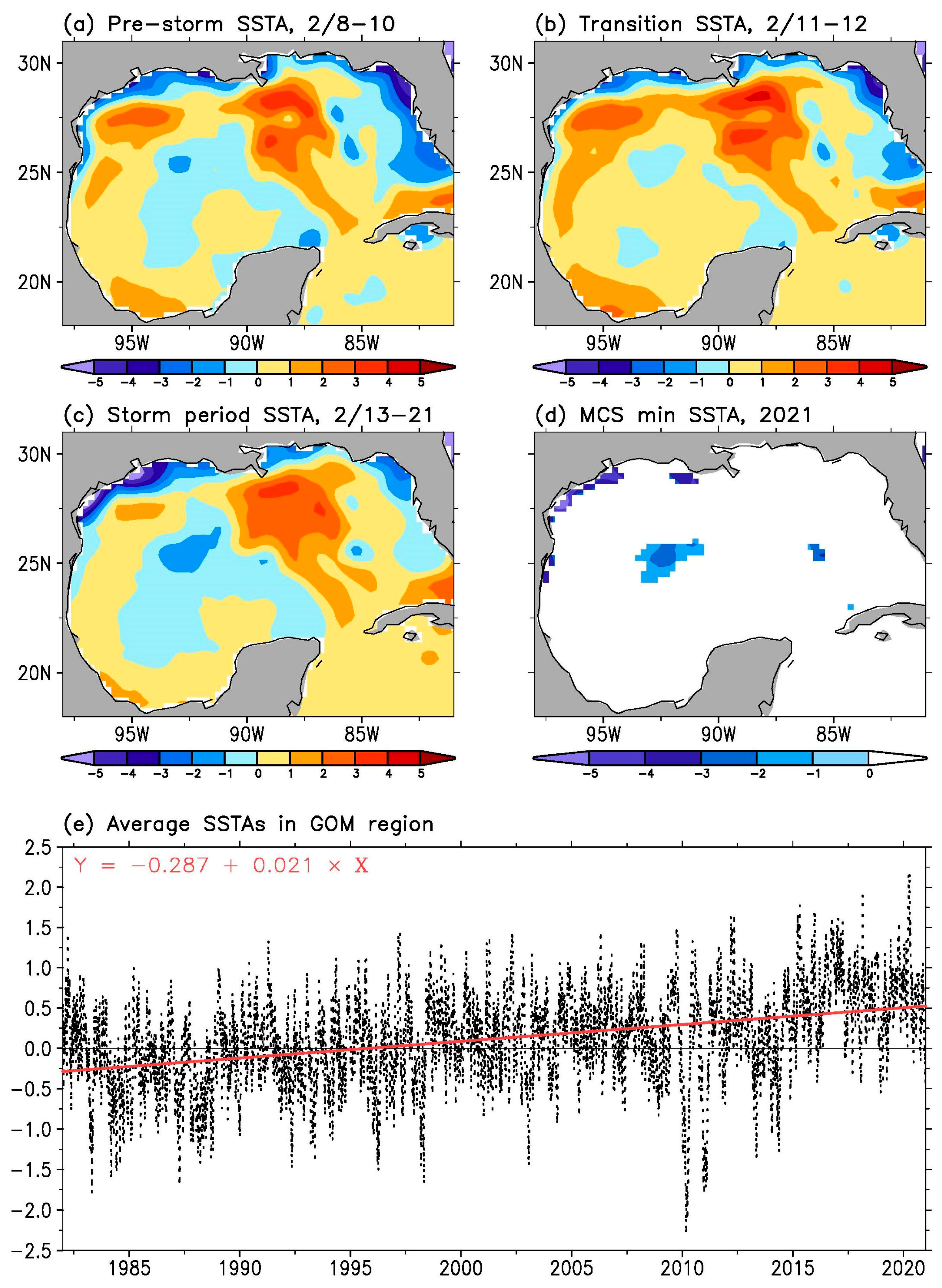
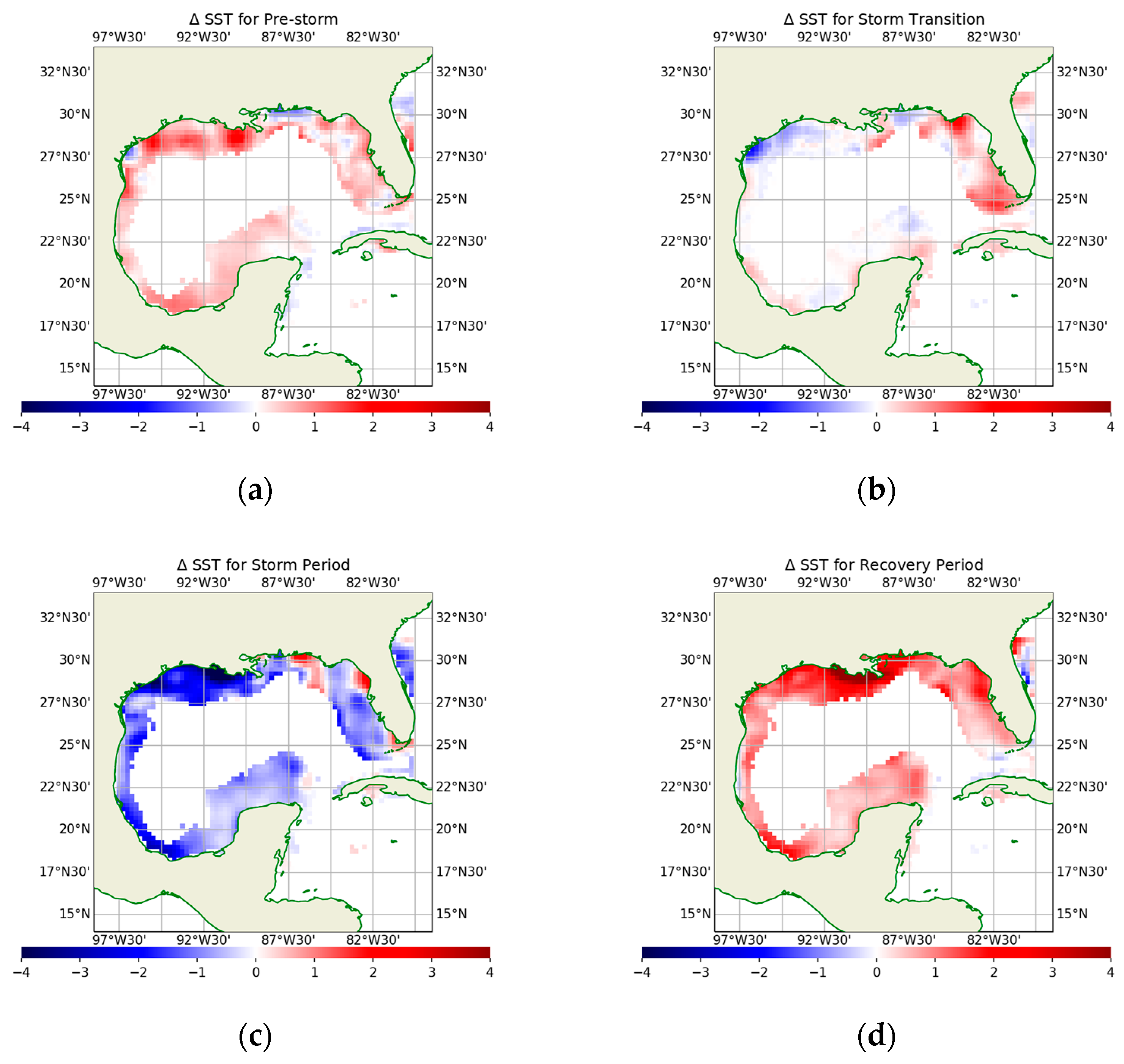
3.2.1. Cooling Caused by WSO21

As described in Section 3.1, WSO21 substantially cooled the western GoM (Figure 4). During the pre-storm period (Period I; Figure 4a), the SSTAs were 1° to 2 °C above normal (the long-term average between 1982 and 2021) in the western GoM, 1° to 3 °C above normal in the central GoM related to the Loop Current position (Figure 2b), −1° to −2 °C below normal along the northwestern coasts of the GoM and −1° to −3 °C below normal along the eastern coasts of the GoM. During Period II (Figure 4b), SSTAs decreased by approximately 0.5 °C near the western coasts of GoM but increased slightly in the central GoM, while cold SSTAs remained in the western, northern and eastern coasts of the GoM. During Period III, (the storm period, Figure 4c), the SSTAs clearly decreased ~3 °C along the northwestern coasts of the GoM, which is consistent with the buoy observations (Table 1 and Figure 3). The SSTAs decreased by approximately 1 °C in the eastern-central GoM but increased by approximately 2 °C along the eastern coasts of the GoM, which is outside of the area that WSO21 impacted.
MCSs, the counterpart to marine heatwaves, which are defined as cold events when SSTs are lower than the 95 percentile SST and sustained for longer than 5 days [41,42], are plotted in Figure 4d. The dropping of the SSTAs triggered strong MCSs (Figure 4d) with minimum SSTAs of −3° to −5 °C along the northwestern coasts and weaker MCSs in the central GoM with minimum SSTAs of −1° to −2 °C. Overall, MCSs were confined to the northwestern coasts of the GoM, while most of the central GoM was MCS-free, which was directly associated with the warmer-than-normal SSTAs during the pre-storm period (Figure 4a) and the warm water transportation by the Loop Current (Figure 2b) into the mid-GoM. The limited MCSs caused by WSO21 in February 2021 were also impacted by the long-term warming trend of the GoM. Figure 4e shows the daily averaged SSTA data for the entire GoM. The linear trend in the anomalies (red line) is overlaid on the anomaly line. The GoM shows a significant increase in SSTA, with temperature increases of ~0.2 °C per decade (p << 0.05) between 1982 and 2021. The trend of SST increase is comparable to estimates in previous studies [18,22,27]. The minimum SSTA each year also increases with time as the overall warming rate increases [18]. The average minimum SSTA after 2015 is approximately 1.0 °C higher than the average minimum before 1990. Note, our data also show the 2010 and 2011 cold events, which have been described in [18,22]. The warmer-than-normal pre-storm SST conditions greatly reduced the chances for the formation of MCSs during WSO21, and are investigated further in the Section 4. Even with a limited area of MCSs, WSO21 still caused significant mortality to sea turtles and fish [11,13].

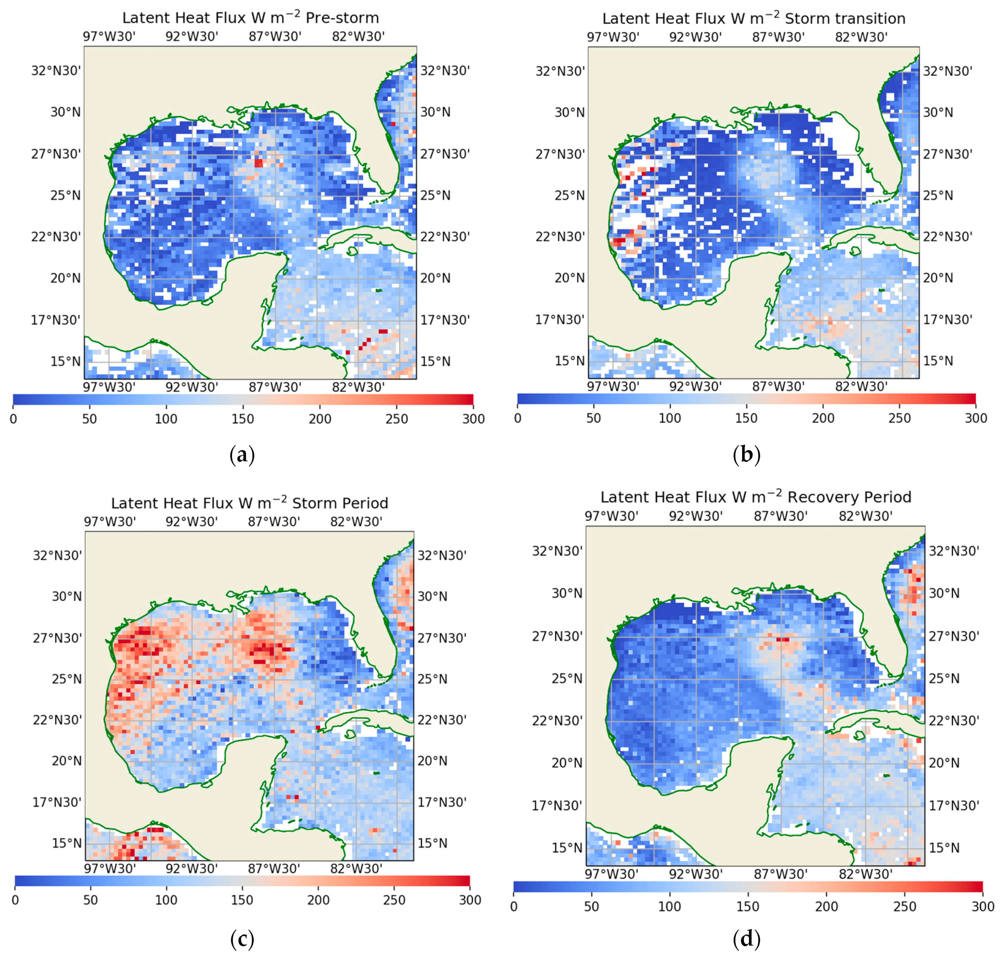
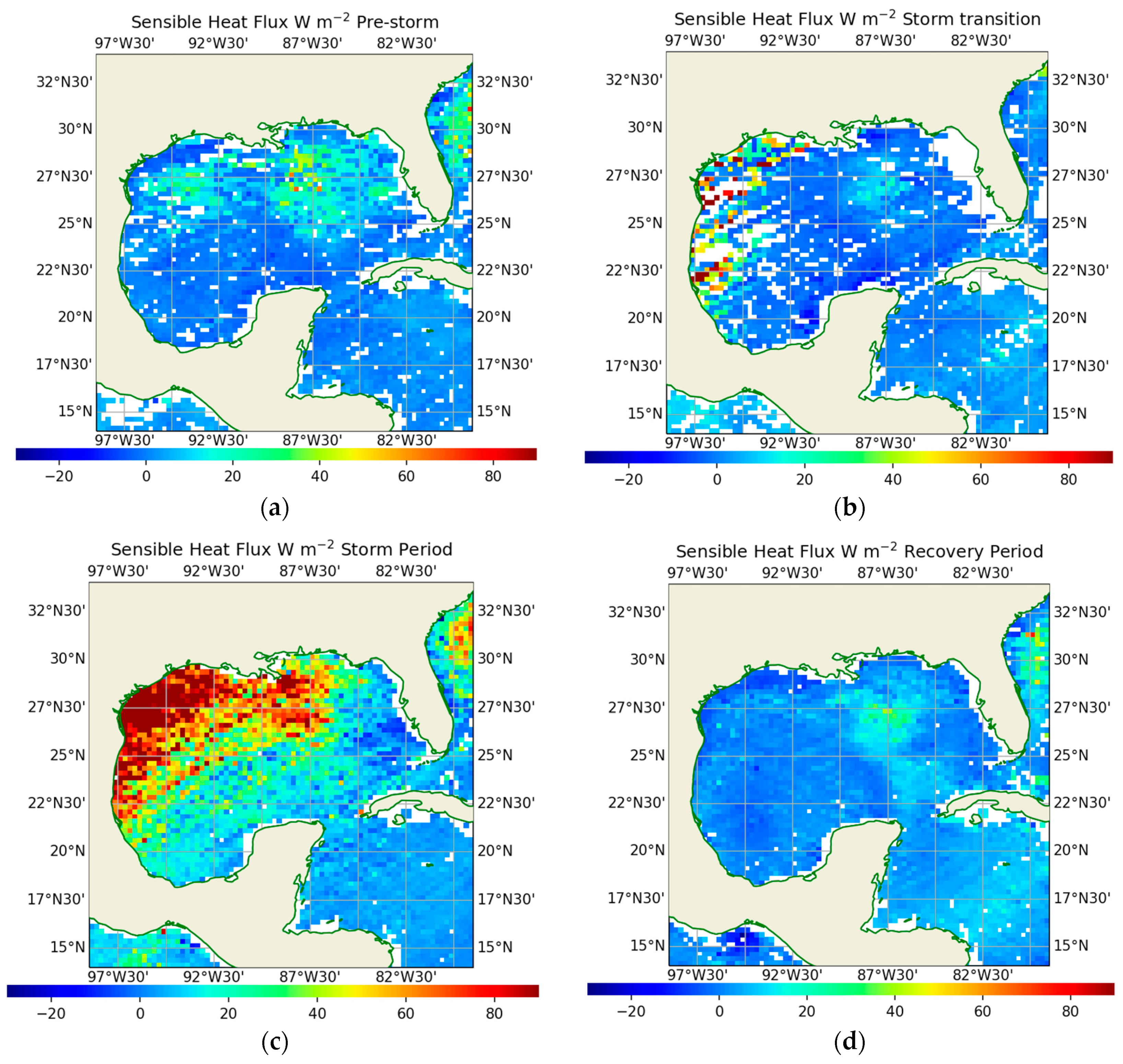
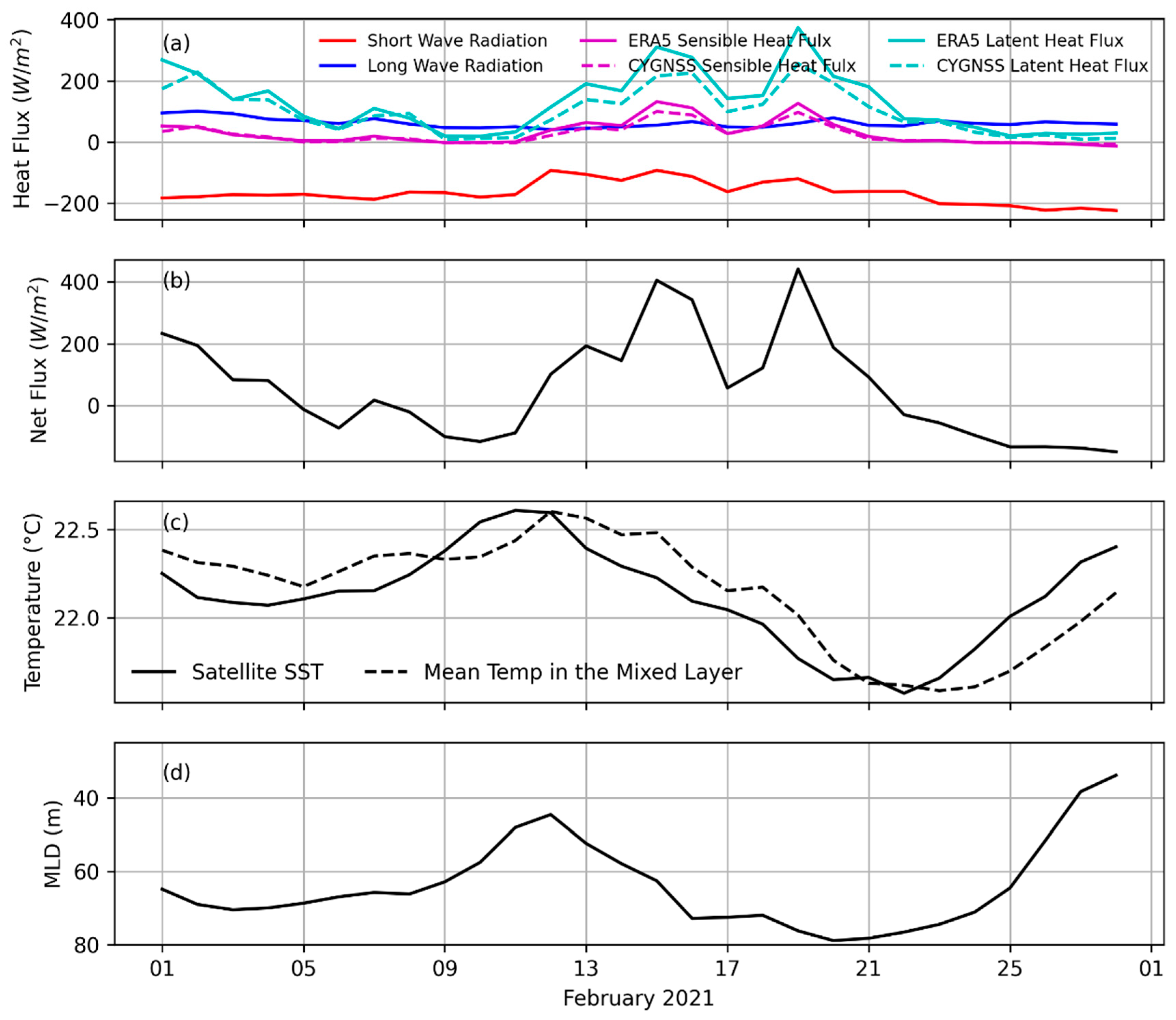
3.2.2. Surface Turbulent Heat Fluxes Response

Surface heat flux is the exchange of heat per unit area between the surface of the ocean and the atmosphere. These fluxes include latent heat flux (LHF) and sensible heat flux (SHF). They play an important role in the genesis and evolution of winter storms. Both the LHF and SHF during the passage of WSO21 were obtained using the CYGNSS data [32]. Large air–sea temperature and humidity differences were observed during the winter season, which were enhanced by winter storms due to the cold and often windy weather associated with them. Figure 5 and Figure 6 show the LHF and SHF, respectively, over the region of interest during the four periods of WSO21. By convention, positive LHF and SHF values indicate upward flux or heat coming out of the ocean, while negative values indicate downward flux, i.e., heat flowing into the ocean.
The CYGNSS heat flux data were validated [32,43] against many global buoy networks including Kuroshio extension (KIO), National Data Buoy Center (NDBC), OceanSITES and tropical moored buoy systems (i.e., TAO, TRITON, PIRATA, RAMA, etc.). Both studies [32,43] showed that CYGNSS validation with the global buoy networks yielded average RMSEs of ~33 to 39 W/m2 and ~6 to 9 W/m2 for LHF and SHF, respectively. The overall bias in CYGNSS LHF data was ~−3.6 W/m2, signifying that the CYGNSS LHF was underestimated when compared to in situ measurements. SHF was slightly overestimated by 1.5 W/m2. These biases and errors were less significant for the Atlantic Ocean compared to the Pacific and Indian Oceans. When compared with ERA5 heat fluxes (plots not shown here), it was observed that during the pre-storm conditions, CYGNSS underestimated by a mean difference of~2 W/m2; this underestimation further increased by ~10 to 14 W/m2 during the storm period and returned to ~5 W/m2 during the post-storm recovery period. This underestimation indicates that the turbulent heat fluxes from CYGNSS yielded less heat loss to the atmosphere compared to that estimated from ERA5 heat fluxes.
From Figure 5a and Figure 6a, one can observe higher LHF and SHF, as expected during winter months. During 8–10 February, when the conditions were pre-storm, LHF along the northwest and west coasts of the GoM (where the cold front entered the GoM) were in the range of 50 to 120 W/m2 with a small region of higher values (~250 W/m2) over the Loop Current area. The corresponding SHF values were within the range of 20 W/m2 to 50 W/m2, with high values over the Loop Current area. During the storm transition (Figure 5b and Figure 6b) phase as the winter storm was near the southeast coast of Texas and about to reach the warm waters of the northwest and western GoM, some sporadic high values of LHF (~220 W/m2) and SHF (40 to 70 W/m2) could be observed. As the cold front moved through the northwestern and western shores of the GoM, carrying very dry and cold winds (air temperatures approximately 10 degrees below the freezing point) over a very moist and relatively warm ocean surface, these large temperature and humidity differences led to abnormally high heat fluxes (LHF > 300 W/m2 and SHF~100 W/m2), which cooled the ocean (Figure 5c and Figure 6c). These higher heat fluxes, associated with very high winds and cold air temperatures, further died down as the multiple cold fronts moved away from the area during the post-storm recovery period (Figure 5d and Figure 6d).

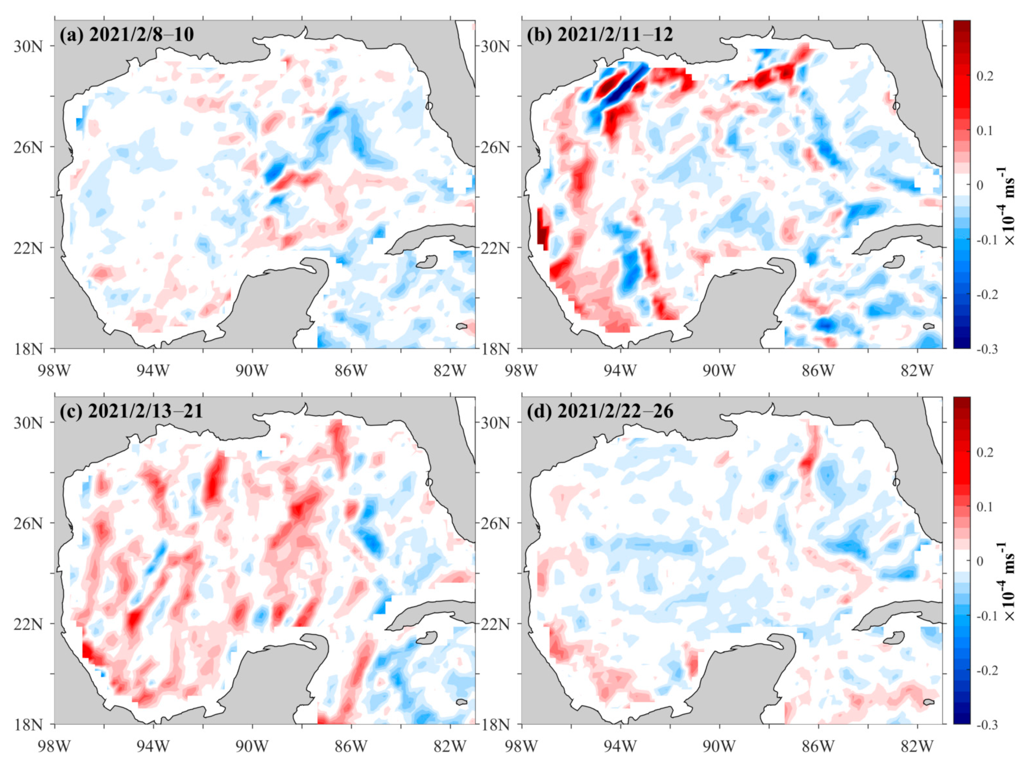
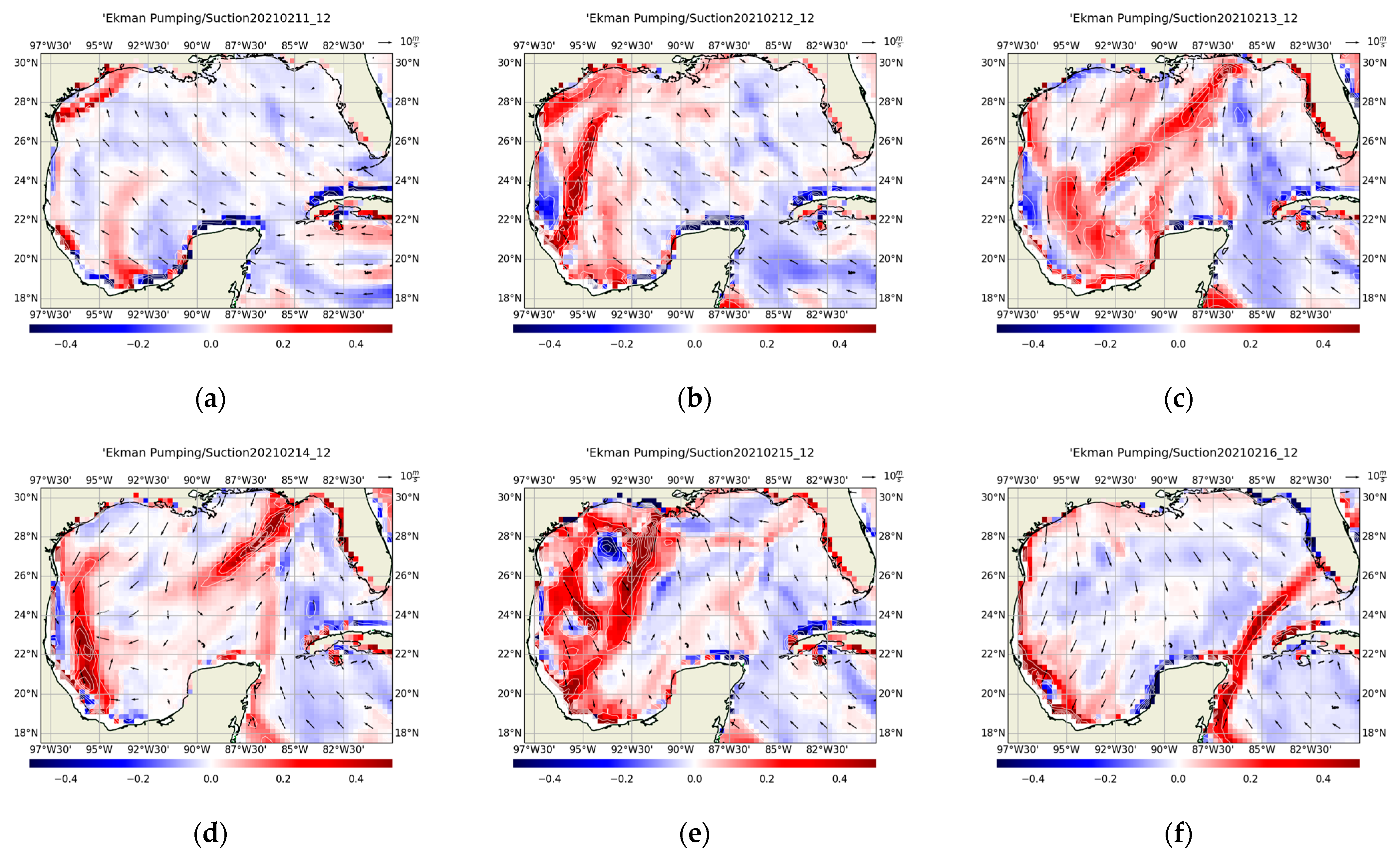
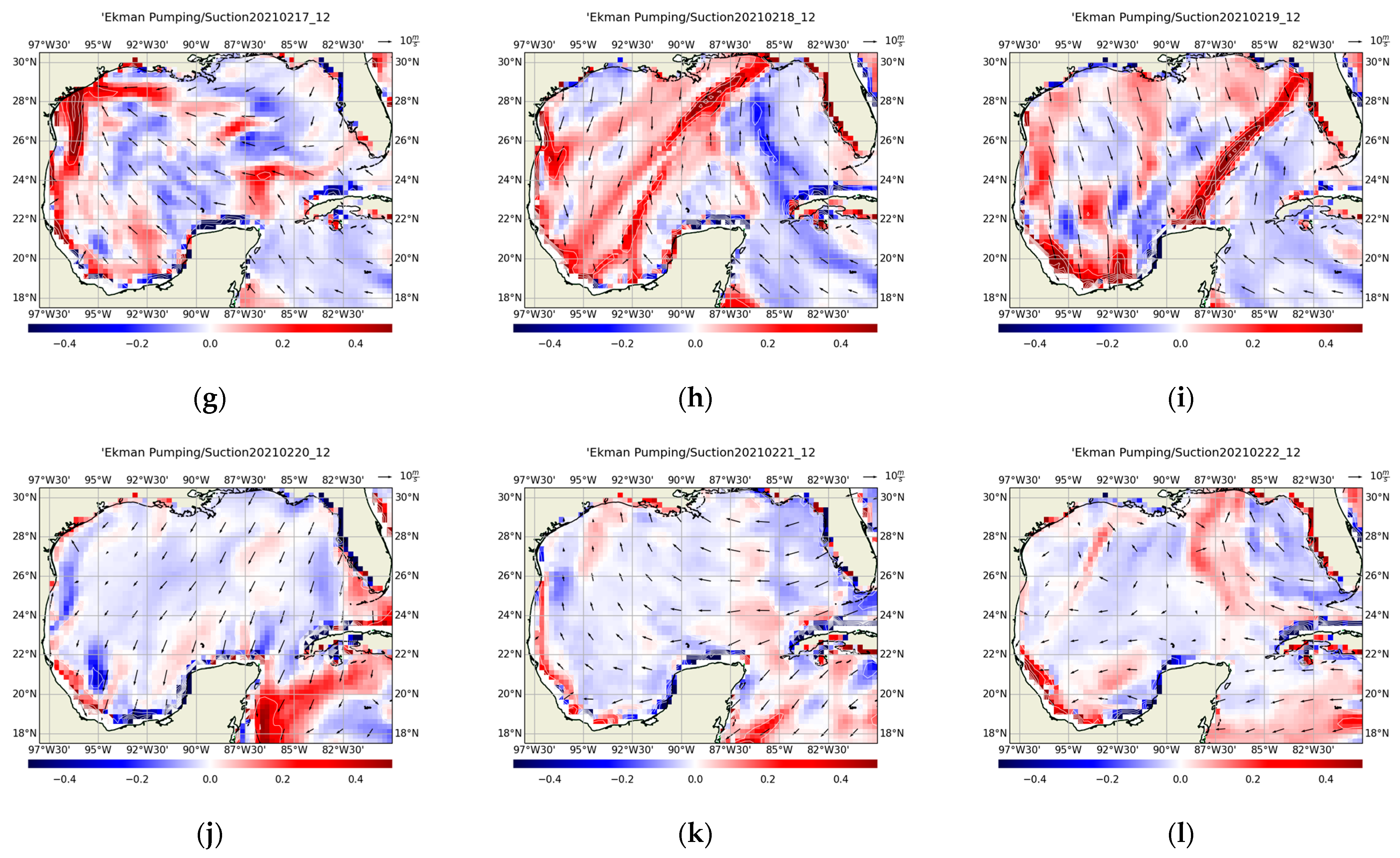
3.2.3. Ekman Suction

Responses of the ocean subsurface to storm conditions can be observed through Ekman pumping/suction due to changes in wind direction and magnitude. Ekman suction is a manifestation of thermocline shoaling/deepening due to changes in the curl of the wind stress. Ekman suction, which occurs when there is a cyclonic rotation of the winds (which is typically associated with storms), brings salty and cooler subsurface waters to the surface ocean of the GoM. Prior to the formation of WSO21 (Figure 7a), Ekman suction was mostly non-existent in most parts of the GoM. As the wind regime changed with the buildup of the storm (Figure 7b), Ekman suction became more noticeable in the western GoM. During Period III (Figure 7c), the cyclonic winds strengthened, causing a greater suction (i.e., upwelling) of cold/salty subsurface waters in most parts of the western GoM. Post WSO21 (Figure 7d), as the winds weakened and changed direction, the entire GoM returned to pre-storm conditions, with very weak Ekman suction.
Figure 7c shows the average Ekman suction during Period III. Upwelling happened almost everywhere in the western GoM (red color). Apart from the sudden cooling due to direct air–sea interaction, this is an important mechanism in helping to cool the near-surface water temperatures, as shown in Figure 3 and Figure 4, and, more importantly, explains the near-coastal salinity and chlorophyll-a increase during WSO21 (shown below). As in Figure 3, the wind magnitude and direction changed rapidly during WSO21; therefore, in Figure 8, we show the daily Ekman suction at 12 UTC to demonstrate the localized upwelling and rapid wind reversal during WSO21. In fact, the wind direction and magnitude could significantly change within hours based on the 6-hourly wind data.
When WSO21 arrived on 11 February 2021, upwelling was observed only in the coastal regions because the dominant wind was mostly southwesterly (Figure 8). The northerly wind then expanded from the coastal northwest GoM to the interior GoM and became the dominant wind in the western GoM on 13 February. Correspondingly, the upwelling zone expanded from the western coastal regions to the entire western GoM from 11 February to 13 February and further expanded to most of the eastern GoM on 14 February. Upwelling occurred along a long divergence zone in the central northern GoM, where the winds of different air masses diverged on 13 and 14 February. The upwelling was strongest and associated with the arrival of the most robust Arctic front of WSO21 on 15 February in the western and northwestern GoM, but was only observed along coastal regions on 16 February. In most regions of the western GoM, the wind on 17 February reversed to southeasterly, still causing strong upwelling along the western coastal regions. Associated with the passage of the third and final cold front during WSO21, on 18 and 19 February, the wind reverted to northerly and upwelling was formed in most regions of the western GoM. As the recovery period built up, the wind direction changed from northerly to southeasterly, with no upwelling in the northwest coastal GoM.
Coastal upwelling was observed almost every day during WSO21 at the northwest corner, where many of the buoys are located. Upwelling is one of the keys to explaining the phenomena observed by those buoys. From Figure 8, we also find that both the intensity and location of the upwelling could change rapidly. It is critical to examine the upwelling using daily or higher resolution wind data to fully understand the chlorophyll-a and salinity change below.
From Figure 8, we can observe that the variability in wind strength and direction was quite high over the storm period, which is indicative of multiple cold fronts related to WSO21 crossing the GoM, as discussed in the Section 1. On 11 February (Figure 8a), there were weak southeasterly winds throughout the GoM, with the first cold front beginning to slide through the northwestern GoM on 12 February (Figure 8b) and fully through the northwestern GoM on 13 February. This can be clearly observed from the wind patterns on 13 February (Figure 8c), with strong northerly winds in the northwestern GoM and southerly winds in the southeastern GoM. In Figure 8d, the front appears to continue to move southeasterly through the GoM on 14 February, with another cold and much stronger front right on its heels, moving through the northwestern GoM on 15 February (Figure 8e). Once again, there was a clear delineation in the wind directions, which marked the location of the front, with cold northwesterly winds on the backside and southerly winds out in front. The front nearly cleared the whole GoM by 16 February, which was illustrated by most of the GoM experiencing northerly winds (Figure 8f). On 17 February, the winds began to return to pre-storm conditions, with southeasterly winds dominating much of the GoM; however, another cold front came through the western GoM, with its presence once again observable in the strong northerly winds on the backside in the western GoM and southerly winds out ahead of it (Figure 8g,h). The front slowly moved through the entire GoM on 19 and 20 February (Figure 8i,j), with pre-storm conditions beginning to prevail in the GoM on 21 and 22 February (Figure 8k,l). The multiple cold fronts that passed through the GoM during the 12 to 20 February time period caused multiple instances of strong northerly winds on the backside of the front, with southerly winds out in front. These repetitive cyclonic rotations in the western half of the GoM led to Ekman suction and, when averaged out during the entire week, we can understand why Ekman suction and thus upwelling dominated much of the western half of the GoM over the storm period (Figure 7c).

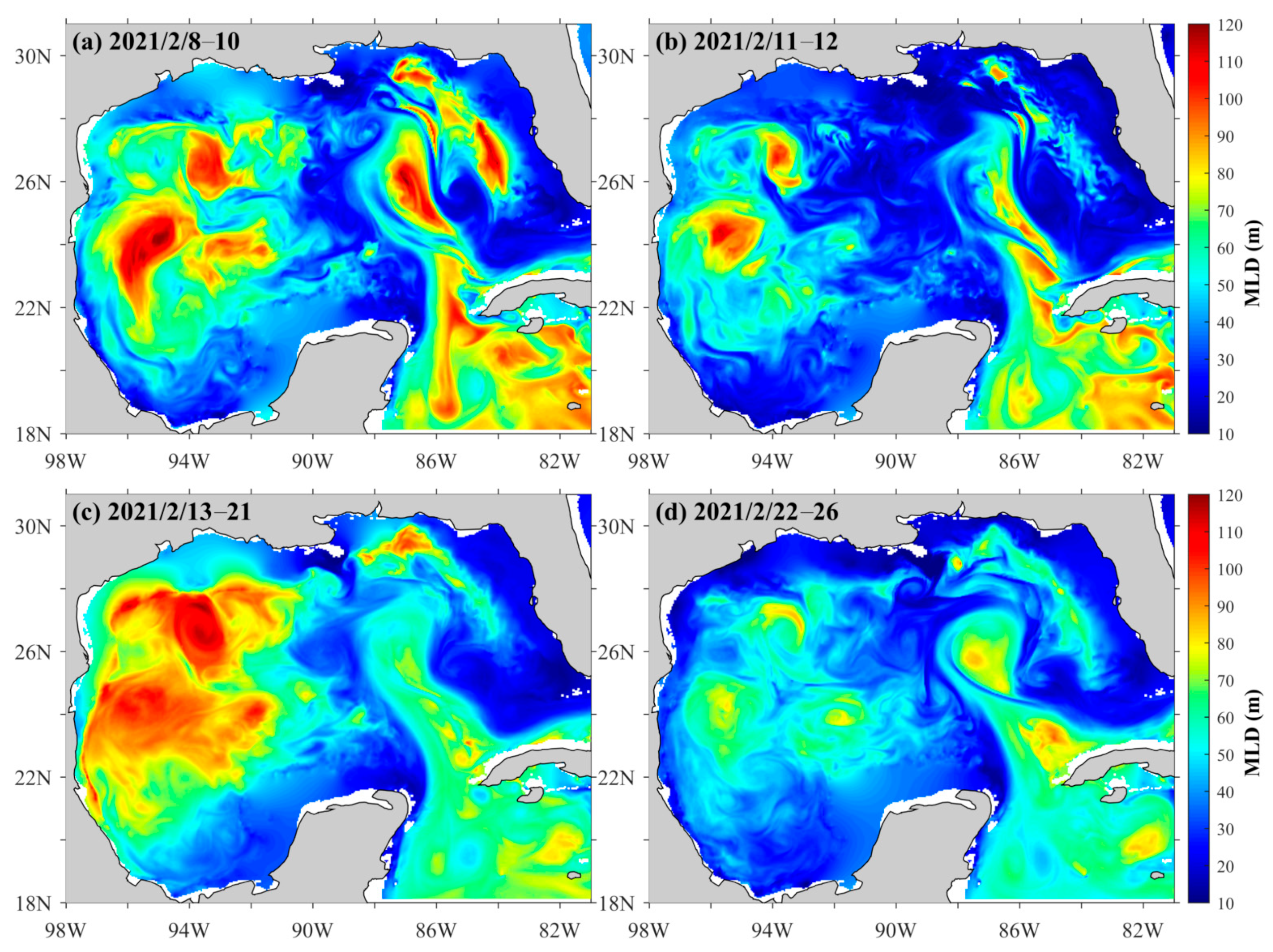
3.2.4. Mixed Layer Depth

The ML is an indicator of turbulent mixing processes that occur in the upper ocean. The response of the ML to conditions during the passage of WSO21 is shown in Figure 9. During the pre-storm phase of WSO21 (Figure 9a), the ML was relatively deep in the western GoM, with a core centered around 95W, 24N. A narrower band of deeper ML was observed in the northeastern GoM. During the transition period (Figure 9b), the MLDs reduced and became more localized. The impacts of storm-related turbulent mixing conditions such as surface forcing (e.g., strong winds and heat fluxes) and lateral advection were clearly noticeable during the WSO21 storm period (Figure 9c). At this time, the MLD was deepened (>100 m) relative to pre-storm conditions and was more widespread, covering nearly the entire western GoM. After the passage of WSO21 (Figure 9d), there was a drastic reduction in the MLD in the entire GoM, reaching values lower than those of pre-storm conditions in many regions of the GoM.

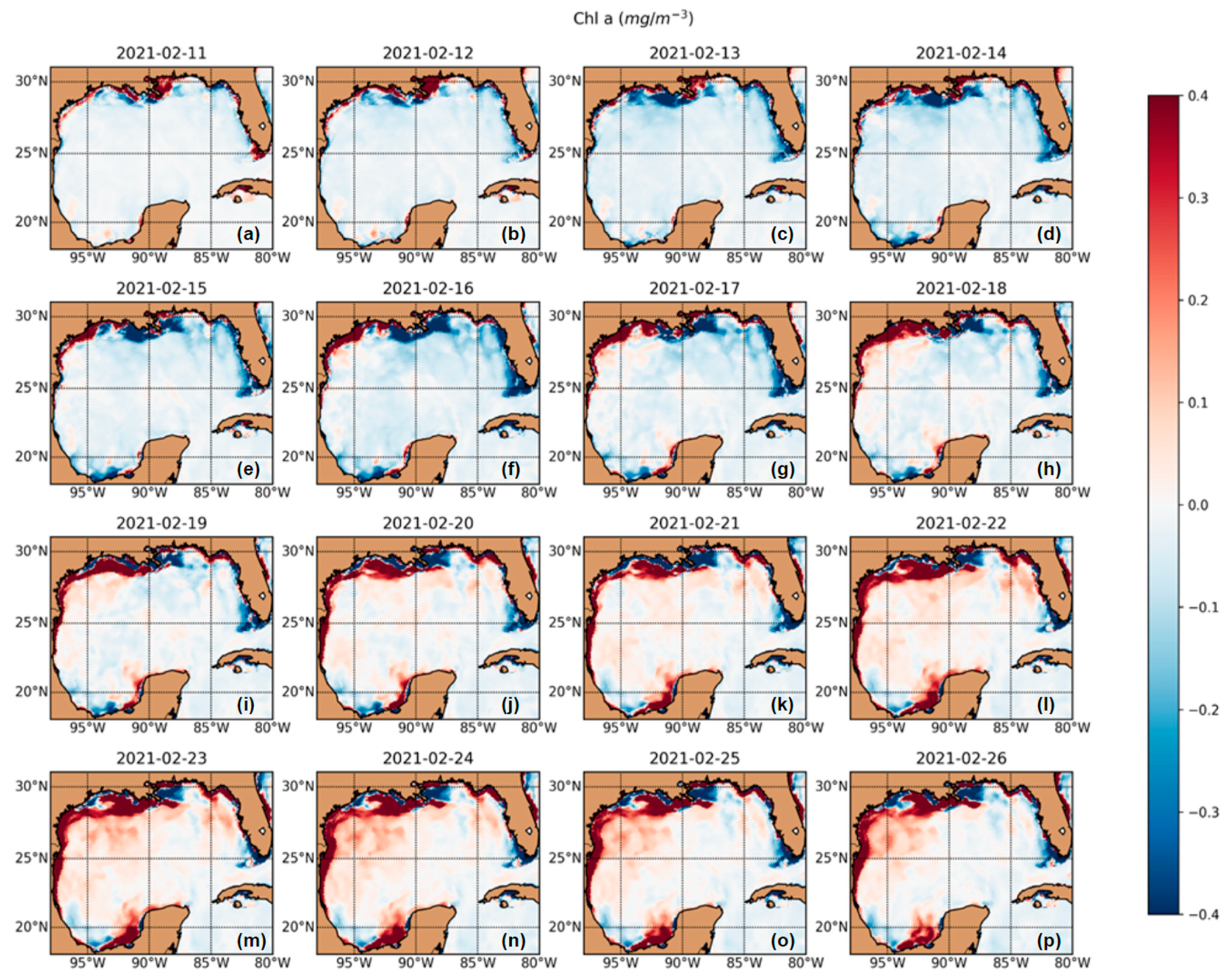
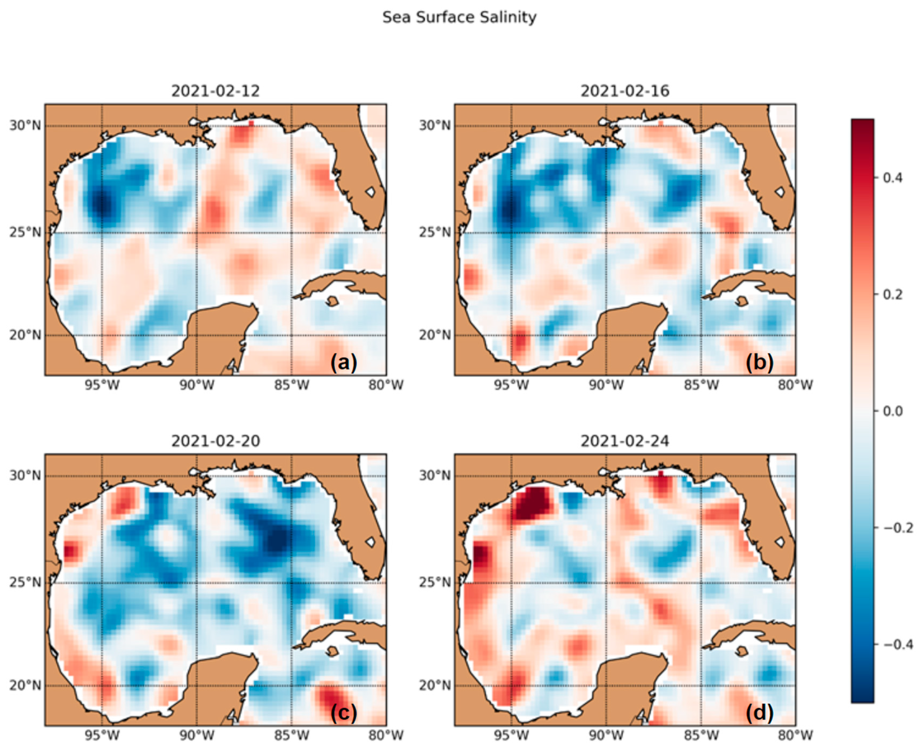
3.2.5. Changes in Ocean Color and Sea Surface Salinity (SSS)

To highlight the changes during WSO21 for ocean color and SSS, we show the changes during Periods II-IV in reference to the pre-storm conditions (average of Period I) in the following analysis. This allows us to show the evolution of chlorophyll-a and SSS during WSO21.
Figure 10 shows the daily changes of chlorophyll-a during WSO21. The changes of chlorophyll-a exhibited a notable decrease along the Mississippi River Delta (MRD) region in the first half of the storm period from 13 to 18 February (Figure 10c–h), corresponding to a warmer water mass (daily SSTA, not shown) and weak downwelling (Figure 8) at that region. The chlorophyll-a in the offshore of the MRD started to increase between 19 and 21 February, and the entire MRD region had enhanced chlorophyll-a from 22 to 26 February (Figure 10i–p). Strong upwelling was observed (Figure 8h,i) on 18 and 19 February, which may have been responsible for the chlorophyll-a increase in the MRD. During the second half of WSO21, anomalous increased chlorophyll-a also occurred along the central northern coast of the GoM (Figure 10k–p, 21–26 February). On the northwestern coast, an increase in chlorophyll-a was visible from 13 to 15 February and became more noticeable with a southward extension along the west coast during WSO21. The location of the coastal chlorophyll-a bloom is consistent with the coastal upwelling zone shown in Figure 8, with an expected time delay. Compared to the wind field and upwelling, accumulation of chlorophyll-a still persisted (Figure 10l–p, 22–26 February) after the wind field recovered from the storm (Figure 7d) and lasted longer. The phytoplankton growth in the GoM is nutrient-limited [22]. For the GoM, chlorophyll-a maximum is usually measured in February [18,22], when upwelling and mixing bring nutrients to the surface and cause phytoplankton growth in the winter in the northern GoM [18]. The chlorophyll-a concentration of the deep western GoM was also slightly increased during the post-storm period (22–26 February) compared to the beginning of WSO21 (11–15 February). Chlorophyll-a enhancement was also found in the western region of the Yucatan Peninsula in the southwest GOM starting from 20 February. It is unclear whether that was WSO21-related.
Because SSS is already a 7-day running mean, we used selected data on 12, 16, 20 and 24 February as representatives in Figure 11 to show the evolution of salinity changes during WSO21. The changes in SSS during the WSO21 storm period were characterized by notable salinity increases along the coastal regions in the western GoM (Figure 11c,d). The salinity increases were generally isolated to some coastal locales on 12 and 16 February (Figure 11a,b), but spread to engulf much of the western GoM coastal region on 20 and 24 February (Figure 11c,d). This is consistent with the coastal upwelling (Figure 8) during WSO21 because the coastal salinity at depth was larger than the salinity in the surface ML (Figure 1). Salinity is a good indicator of upwelling in the coastal region of the western GoM. Upwelling and mixing bring salty water from the base of the ML, as evident from the climatological mean values of salinity in February (Figure 1b,c), to the surface and can cause the salinity to increase in the coastal regions in the western GoM. This is also consistent with the coastal chlorophyll-a increase shown in Figure 10.
Another prominent feature during WSO21 was the reduction of salinity in the northwestern GoM centered around 95°W, 27°N during the beginning of WSO21 (Figure 11a,b). WSO21 brought some precipitation to the GoM from 11 to 18 February (Figure 12), which may have been responsible for the interior northwestern GoM sea surface salinity reduction shown in Figure 11. The satellite SSS freshening may be linearly correlated to the rain rate [44,45]. The regions near the Mississippi River plume and the coastal regions usually have low salinity waters. Offshore advection can also bring low coastal water to the interior and cause a salinity decrease in the open ocean in the GoM.

4. Discussion

4.1. Cooling in the Western GoM

To understand the processes that led to the GoM cooling during WSO21, we show the average short-wave radiation, long-wave radiation, sensible heat flux and latent heat flux for the western GoM in February 2021 (Figure 13a; positive: losing heat to the atmosphere; negative: gaining heat in the ocean). The area averaged for Figure 13 is shown by the white rectangle in Figure 2b, which was the area most impacted by WSO21. Although long-wave radiation did not change significantly during WSO21, the magnitude of the short-wave radiation rapidly reduced from ~200 W/m2 to less than 120 W/m2 with the arrival of WSO21 on 12 February 2021. Sensible heat flux also changed from near 0 to 30–50 W/m2, which is consistent with Figure 5. The most noteworthy change was in latent heat flux, which increased from near 0 to more than 250 W/m2 during WSO21. Both sensible and latent heat fluxes from ERA5 and CYGNSS showed the arrival and movement of the three cold fronts, as indicated by the buoy data in Figure 3 and wind data in Figure 8. The magnitude of the CYGNSS turbulent heat fluxes was slightly lower than those estimated by ERA5 during WSO21. The net surface heat flux (Figure 13b) was obtained by the sum of the four ERA5 heat flux components shown in Figure 13a. Before the arrival of WSO21 between 5 and 11 February, the net surface heat flux was mostly negative, which suggests the ocean was gaining heat from the atmosphere. During WSO21 and its associated cold fronts, cooling continued to occur in the immediate aftermath of each passing front. With the passage of the first two fronts on 2/11 and 2/14, there was a rapid net surface heat flux change from −50 W/m2 to more than 250 W/m2 over just a few days (11–15 February, Figure 13b). With the passage of each front, the ocean continued losing heat to the atmosphere until the remnants of the final cold front associated with WSO21 (which passed through on 17 February) were no longer impacting the GoM (21 February). The SST averaged over the western GoM (Figure 13c) demonstrates the cooling impact from net surface heat flux on the surface ML. The SST was highest during the transition period (11–12 February), with values of more than 22.5 °C, which was at least partly due to the negative net surface heat flux before WSO21 (gaining heat). The SST then continuously declined from 12 to 21 February during the storm period of WSO21 as the ocean heat was lost to the atmosphere (Figure 13b). The average SST in the western GoM dropped by ~1 °C in 11 days during WSO21. The average ML temperature and MLD were estimated from HYCOM (Figure 13c,d). The ML temperature showed a very similar trend and magnitude as SST but lagged by approximately 1 day, suggesting that it takes approximately a day for the entire ML to have the same temperature as the surface. In response to pre-storm warming, the MLD was shallower (~44 m) when WSO21 arrived (transition period, 11–12 February). The ML deepened during WSO21 (Figure 13d), which is consistent with the deepening shown in Figure 9.
The heat loss (cooling) and SST change could be investigated using a simple heat budget balance.
H l o s s = ρ w C p Δ T A h   d t
where H l o s s is the accumulated total heat loss from the ocean to the atmosphere during WSO21, which can be estimated from the net surface heat flux (Figure 13b). During WSO21, approximately 1.41 × 10²⁰ J of heat was lost to the atmosphere between 11 and 21 February, with the study area being ~7.81 × 10¹¹ m2 (A; the area of the white rectangular in Figure 2). ρ w = 1026 kg/m3 is the water density and C p = 3995   J / kg / °C is the ocean heat capacity. ∆ T is the average water temperature change in the surface ML during WSO21 and h is the thickness of the water column that can be cooled down due to surface heat loss. Finally, dt is the integral time step, which is from 11 to 21 February. Both SST and average MLD temperature suggested a ~1.0 °C temperature decrease over this area during WSO21 (Figure 13c). If we use Δ T = 1.0 °C from Figure 13c in Equation (5), this yield h = 42.9   m. This calculation suggests that the heat loss to the atmosphere during WSO21 in the western GoM could reduce the temperature in the upper 42.9 m by 1.0 °C. If the deepest ML around 20 February is considered (h = ~80 m), the same amount of heat loss could reduce the entire 80 m of ML temperature by 0.54 °C, which is more than half of the total temperature decrease (~1.0 °C) during WSO21. Thus, more than half of the temperature drop can be explained by net surface heat loss.
The cooling in the upper 42.9 m (the initial MLD in the transition period) can be fully explained by the surface heat loss during WSO21, but there was more heat loss below the initial MLD due to ML deepening. Because the MLD was almost doubled during WSO21, the ocean heat content in the ML was not conserved. Knowing the net surface heat flux could not yield a full explanation of the subsurface cooling in the ML during WSO21 means the rest of the heat change should be due to entrainment, wind mixing, diffusion, upwelling, horizontal mixing and advection. Those cannot be quantified without a full heat budget model, which is beyond the scope of this paper. Nonetheless, using the surface heat flux, we quantified the role of surface cooling, which should be responsible for at least 54% of the temperature decrease during WSO21 when even the deepest MLD is considered. The surface heat loss was the dominant process controlling the cooling.

4.2. Coastal Cooling during WSO21

Dramatic temperature declines were observed in the coastal regions during WSO21 (Figure 3 and Figure 4). To understand the magnitude of the cooling and its spatial extent in the coastal regions, the DOISST data were used. The daily data were used to estimate the rate of change of SST per unit day and then accumulated along the four prominent storm periods to estimate the cumulative change in SST (ΔSST). As most of the cooling was observed in the coastal region of the GoM, where the largest loss of marine life was reported [11,13], we plotted (in Figure 14) only the coastal region, using a mask where the bathymetry data are <1000 m. During the pre-storm period, there was an increase in SST transitions into slight cooling during the transition phase. As the winter storm hit the western GoM shoreline, the sudden cooling began, and remained for the whole storm period (11 days), with a maximum cooling of ~5 °C mostly isolated to the northwest and southwest coasts of the GoM. This cooling of ~5 °C agrees with data from the three in-situ stations (42035, 42092, 42048), which are located very near the coast (Figure 3f). There is also one location (PTAT2/ANPT2) very close to the coastline where the SST dropped by 10 °C. We did not observe such a drop in the satellite data due to land contamination, where the gridded data were unable to resolve the data so close to the coast. It is possible that the juvenile green turtles, which are mostly found nearshore of coastal Texas (a foraging habitat), were hypothermia stunned as the temperatures dropped ~5 to 10 °C along the coastal inshore waters. These western coasts of GoM also had an abundance of forage and game fish that also died in significant numbers. As the storm left the GoM, the temperatures began to increase and head back towards normal temperatures, as shown in the recovery period (Figure 14d).

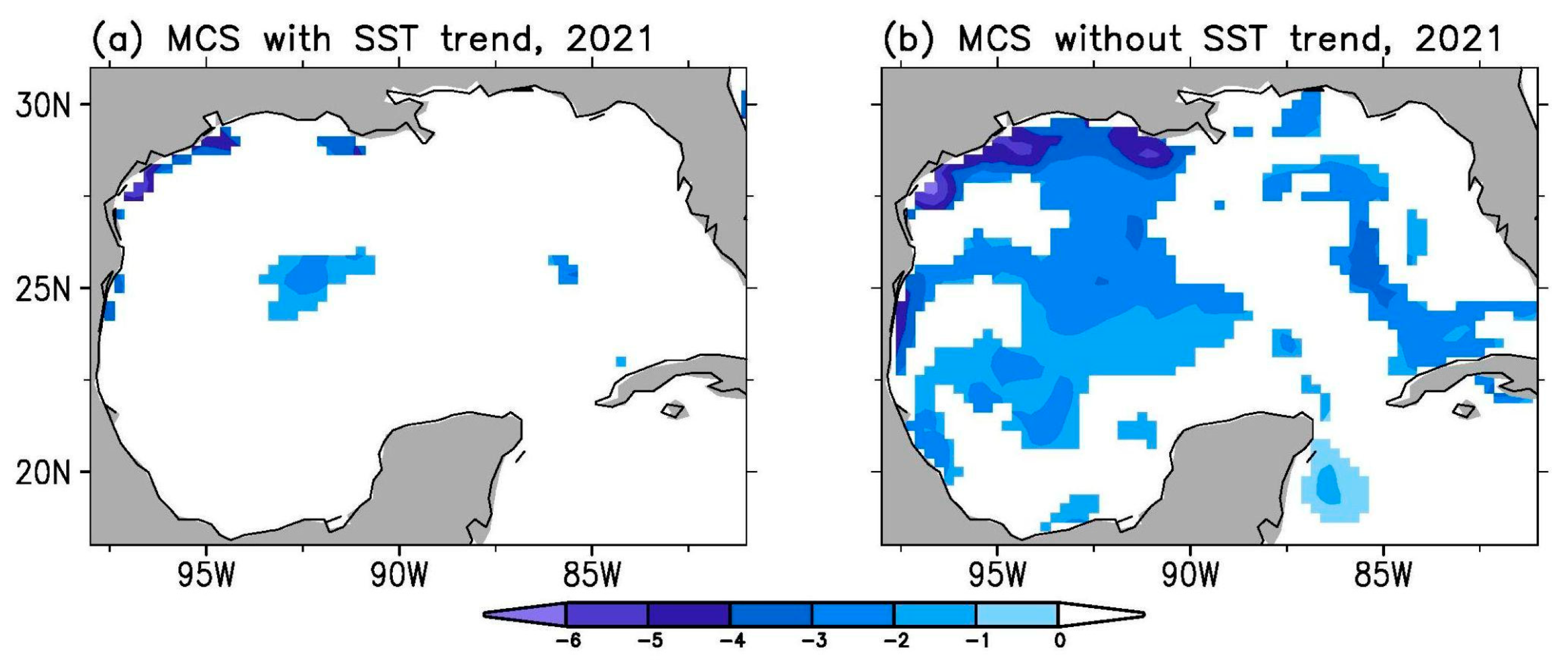
4.3. Global Warming Impact on WSO21

Recent studies have found that GoM SST is warming faster than the global ocean at a rate of approximately 0.2 °C/decade [18,27]. The SST warming began in the 1970s and the average SST has increased approximately 1.0 °C in the past 50 years. Li et al. [18] found that the warming rate in the winter time is slower (at 0.05 °C/decade) than that in summer. Before the arrival of WSO21, the GoM SST was 1–2 °C warmer than the climatological average. The pre-storm warmer-than-normal SST helped to reduce the formation of MCS. MCSs were only formed in the north/northwestern coastal regions and some isolated spots, as shown in Figure 15a. To quantify the impact of GoM warming on cold spell formation, we removed the warming effect on SST by detrending the SST data and recalculating the MCS based on this detrended SST. The detrending process removed a linear trend in SST to make the data collected in 2021 comparable to those collected during historical winter storm events. The trend in SST was mostly due to global warming [18,27], but multi-decadal variations might also have contributed to the long-term trend. Figure 15b shows the distribution of cold spells in February 2021, assuming there was no background warming in the GoM. In reality (Figure 15a), MCS only formed in approximately 14% of the area west of 90W. However, MCS could form in 74% of the area west of 90°W if the warming effect were removed in SST. This comparison indicates that the severity of WSO21 was greatly reduced due to the warming over the last several decades in the GoM. MCS from the detrended SST should be used when comparing data with any historical winter storms before the 1970s. This is also consistent with the findings of Muller-Karger et al. [22] that cooler winters were less frequent in the 2000s than in the 1980s in the GoM, which is likely due to surface warming.

5. Summary

Studies on the oceanic responses to winter storms in the GoM are infrequent and most previous studies have only focused on the biological impacts and fish-killing events caused by winter storms [8,9]. This is partially due to the lack of observations during winter storms in the GoM. In this study, using both in situ and satellite-based datasets, we conducted a comprehensive analysis of changes in different oceanographic parameters before, during and after WSO21, with the goal of advancing our understanding of winter storm impacts in the GoM. Our analysis indicates that oceanic responses to winter storms can be derived from a combination of in situ and satellite observations. In contrast to satellite SST, buoy in situ observations are able to provide more localized details about SST changes during WSO21. For example, the shallowest buoy stations showed that the maximum SST decrease could be greater than 10 °C, but satellite SST underestimated the temperature decline in very shallow waters due to the relatively coarse resolution of satellite data and the dynamical nature of coastal water. However, satellite data are very powerful and advantageous over in situ data as they captured the large-scale changes during WSO21 and provided us with both the temporal and spatial evolutions of water properties during a winter storm.
February is the coldest month [18] in the GoM and WSO21 happened between 11 and 21 February. Three atmospheric fronts brought by WSO21 were the main drivers of the oceanic changes: extreme cold air temperature and enhanced northerly dry wind. Freezing air temperatures during WSO21 caused sea surface cooling (Figure 4, Figure 14 and Figure 15) in the western GoM, which was evident through surface turbulent heat flux increase (Figure 5 and Figure 6) and net surface heat loss (Figure 13). Both higher-than-normal sensible and latent heat flux accounted for the large amount of heat loss during the passage of the cold fronts over the northwestern GoM. Convective mixing subsequently occurred because of overturning density formed at the sea surface by cooling, which effectively deepened the surface ML (Figure 9) and mixed up cooler, saltier and high-nutrient subsurface water from the shallow western GoM coast to the surface.
Before WSO21 arrived, the winds were generally “warming winds” coming from the south; however, with each passing cold front associated with WSO21, southerly winds to the east of the front and northerly winds to the west created strong cyclonic winds that led to the vertical suction of cold, salty water and the mixing of physical and biogeochemical properties in the surface ML. Although there were wind reversals associated with each passing front during WSO21, northerly winds were the dominant wind direction during the storm period. Coastal upwelling was also generated by winds during WSO21 (Figure 8) as there were multiple days with strong offshore winds. This manifested in both chlorophyll-a and salinity increases about 1 week after WSO21 arrived (Figure 10 and Figure 11). Based on the buoy observations, the wave height showed significant increases during WSO21, with maximum values four times larger than values of the pre-storm period.
The long-term trend of SSTA between 1982 and 2021 suggests that the sea surface water in the GoM increased at a rate of approximately 0.2 °C/decade (Figure 4). Warming in the GoM started in the 1970s [27], with the average SST in recent decades being approximately 1.0 °C higher than that in the 1970s. The daily SSTA implies that the temperature in the deepwater of the western GoM is warmer than normal, but the coastal regions were cooler than normal during WSO21. Therefore, marine cold spells are formed mainly in coastal regions in the western GoM (Figure 4). Although sea surface cooling was clearly observed in the deepwater during WSO21, cold spells only formed in a small region centered at 25°N, 92°W in the open ocean. During WSO21, the higher-than-normal SSTA in the eastern GoM showed a strong anticyclonic northern extension of the Loop Current Circulation, which also indicated the presence of a deep layer of warmer water. The northern extension of the Loop Current played an important role in reducing the WSO21 cooling effect in the eastern GoM. MCS from detrended SST also showed that the area of MCS could have been much larger if there had been no warming in recent years (Figure 15).
More than 12,000 cold-stunned sea turtles were rescued, of which only 35% survived, and at least 3.8 million fish were killed along the Texas coast during WSO21 [13]. These dramatic biological impacts can occur when significant water temperature drops occur in coastal regions, such as those caused by WSO21. Besides the initial sudden temperature drops when WSO21 first arrived, the evidence from buoys, satellite SST and wind data indicate that there were multiple cold fronts during WSO21 reinforcing the cold conditions. We suspect that the damaging cold waves were the main cause of the loss of marine life, which resulted in rapid decreases in SST, as was evident from the increase in heat fluxes. The speed, number and strength with which the cold fronts strike in a given amount of time should be an influencing parameter determining the mortality of fish and other marine animals, which may not be detected by satellite data only. Therefore, to complement satellite observations, more in situ observations are needed to measure the changes in near-coast waters along the GoM’s long coast lines.

Author Contributions

Conceptualization, methodology, validation, formal analysis, investigation, data curation, writing—original draft preparation, writing—review and editing, visualization, Z.W., K.S., E.S.N., Y.Z., B.H. and J.R.; project administration, K.S. and Z.W. All authors have read and agreed to the published version of the manuscript.

Funding

This research is supported by National Centers for Environmental Information, NOAA. E.S.N. was partly supported by an Early-Career Research Fellowship from the Gulf Research Program of the US National Academies of Sciences, Engineering, and Medicine (Grant agreement # 2000012639).

Data Availability Statement

The data used in this study are available through various publicly accessible databases. Surface buoy data were obtained from the NBDC (https://www.ndbc.noaa.gov/, accessed in 15 July 2022) and TABS (https://tabs.gerg.tamu.edu/, accessed in 15 July 2022). OISST data are available at https://www.ncei.noaa.gov/products/optimum-interpolation-sst (accessed in 1 June 2022). The CYGNSS latent and sensible heat flux data were obtained through https://podaac-opendap.jpl.nasa.gov/opendap/allData/cygnss/L2/fluxes/cdr_v1.1/, accessed in 5 July 2022). ERA5 surface heat flux is available at https://cds.climate.copernicus.eu/cdsapp#!/dataset/reanalysis-era5-single-levels?tab=overview (accessed in 13 February 2023). The chlorophyll-a concentration data were downloaded from the NOAA CoastWatch website (https://oceanwatch.noaa.gov/cwn/products/noaa-msl12-ocean-color-science-quality-viirs-multi-sensor-snpp-noaa-20-chlorophyll-dineof.html, accessed in 3 July 2022). OISSS data are from http://iprc.soest.hawaii.edu/users/oleg/oisss/GLB/ (accessed in 3 July 2022). HYCOM is available at https://www.hycom.org/data/gomu0pt04/expt-90pt1m000 (accessed in 1 July 2022).

Acknowledgments

The Aquarius/SMAP combined SSS dataset was produced by the International Pacific Research Center (IPRC) of the University of Hawaii, in collaboration with Remote Sensing Systems (RSS), Santa Rosa, CA, and sponsored by the NASA Ocean Salinity Science Team.

Conflicts of Interest

The authors declare no conflict of interest.

References

  1. Cohen, J.; Agel, L.; Barlow, M.; Garfinkel, C.I.; White, I. Linking Arctic Variability and Change with Extreme Winter Weather in the United States. Science 2021, 373, 1116–1121. [Google Scholar] [CrossRef] [PubMed]
  2. Schlegel, R.W.; Darmaraki, S.; Benthuysen, J.A.; Filbee-Dexter, K.; Oliver, E.C.J. Marine Cold-Spells. Prog. Oceanogr. 2021, 198, 102684. [Google Scholar] [CrossRef]
  3. Doss-Gollin, J.; Farnham, D.J.; Lall, U.; Modi, V. How Unprecedented Was the February 2021 Texas Cold Snap? Environ. Res. Lett. 2021, 16, 064056. [Google Scholar] [CrossRef]
  4. Hellerstedt, J. February 2021 Winter Storm-Related Deaths—Texas; Texas Health and Human Services: Austin, TX, USA, 2021. Available online: https://www.dshs.texas.gov/sites/default/files/news/updates/SMOC_FebWinterStorm_MortalitySurvReport_12-30-21.pdf (accessed on 15 July 2022).
  5. Watson, K.P.; Cross, R.; Jones, M.P.; Buttorff, G.; Granato, J.; Pinto, P.; Sipole, S.L.; Vallejo, A. The Winter Storm of 2021. 2021. Available online: https://uh.edu/hobby/winter2021/storm.pdf (accessed on 15 July 2022).
  6. Yang, L.; Liu, M. 2021 February Texas Ice Storm Induced Spring GPP Reduction Compensated by the Higher Precipitation. Earths Future 2023, 11, e2022EF003030. [Google Scholar] [CrossRef]
  7. Nielsen-Gammon, J.W. Chapter 2. The Changing Climate of Texas. In The Impact of Global Warming on Texas; University of Texas Press: Austin, TX, USA, 2011; pp. 39–68. [Google Scholar]
  8. Gunter, G. Death of Fishes Due to Cold on the Texas Coast, January, 1940. Ecology 1941, 22, 203–208. [Google Scholar] [CrossRef]
  9. Gunter, G.; Hildebrand, H.H. Destruction of Fishes and Other Organisms on the South Texas Coast by the Cold Wave of January 28–February 3, 1951. Ecology 1951, 32, 731–736. [Google Scholar] [CrossRef]
  10. Moore, R.H. Observations on Fishes Killed by Cold at Port Aransas, Texas, 11–12 January 1973. Southwest Nat. 1976, 20, 461–466. [Google Scholar] [CrossRef]
  11. Texas Parks and Wildlife. 2021 Winter Storm Coastal Fisheries Impacts; Texas Parks and Wildlife Department: Austin, TX, USA, 2021.
  12. Mollenhauer, R.; Lamont, M.M.; Foley, A. Long-term Apparent Survival of a Cold-stunned Subpopulation of Juvenile Green Turtles. Ecosphere 2022, 13, e4221. [Google Scholar] [CrossRef]
  13. Burnett, J. Texas ‘Cold-Stun’ of 2021 Was Largest Sea Turtle Rescue in History, Scientists Say. Natl. Public Radio 2021. Available online: https://tinyurl.com/Texas-Cold-Stun-Of-2021 (accessed on 22 June 2022).
  14. Proffitt, E.; Devlin, D. Effects of Winter Storm Uri (2021) on Coastal Wetlands: Changes in Marsh-Mangrove Dominance, Soil Properties, Elevation, and Shoreline Retreat at Texas Sentinel Sites. In Proceedings of the Gulf of Mexico Conference, Baton Rouge, LA, USA, 25–28 April 2022. [Google Scholar]
  15. Müller-Karger, F.E.; Walsh, J.J.; Evans, R.H.; Meyers, M.B. On the Seasonal Phytoplankton Concentration and Sea Surface Temperature Cycles of the Gulf of Mexico as Determined by Satellites. J. Geophys. Res. 1991, 96, 12645. [Google Scholar] [CrossRef] [Green Version]
  16. González, N.M.; Müller-Karger, F.E.; Estrada, S.C.; Pérez de los Reyes, R.; del Río, I.V.; Pérez, P.C.; Arenal, I.M. Near-Surface Phytoplankton Distribution in the Western Intra-Americas Sea: The Influence of El Niño and Weather Events. J. Geophys. Res. 2000, 105, 14029–14043. [Google Scholar] [CrossRef]
  17. Villanueva, E.; Mendoza, V.; Adem, J. Sea Surface Temperature and Mixed Layer Depth Changes Due to Cold-Air Outbreak in the Gulf of Mexico. Atmósfera 2010, 23, 325–346. [Google Scholar]
  18. Li, G.; Wang, Z.; Wang, B. Multidecade Trends of Sea Surface Temperature, Chlorophyll-a Concentration, and Ocean Eddies in the Gulf of Mexico. Remote Sens. 2022, 14, 3754. [Google Scholar] [CrossRef]
  19. Spies, R.B.; Senner, S.; Robbins, C.S. An Overview of the Northern Gulf of Mexico Ecosystem. Gulf Mex. Sci. 2016, 33, 9. [Google Scholar] [CrossRef]
  20. Seidov, D.; Mishonov, A.V.; Boyer, T.P.; Baranova, O.K.; Nyadjro, E.; Cross, S.L.; Parsons, A.R.; Weathers, K.W. Gulf of Mexico Regional Climatology, Regional Climatology Team, NOAA/NCEI. Dataset. 2020. Available online: https://www.ncei.noaa.gov/products/gulf-mexico-regional-climatology (accessed on 1 September 2022).
  21. Boyer, T.P.; Baranova, O.K.; Coleman, C.; Garcia, H.E.; Grodsky, A.; Locarnini, R.A.; Mishonov, A.V.; Paver, C.R.; Reagan, J.R.; Seidov, D.; et al. World Ocean Database 2018. A. V 2018. Available online: https://www.ncei.noaa.gov/access/world-ocean-database-select/dbsearch.html (accessed on 1 September 2022).
  22. Muller-Karger, F.E.; Smith, J.P.; Werner, S.; Chen, R.; Roffer, M.; Liu, Y.; Muhling, B.; Lindo-Atichati, D.; Lamkin, J.; Cerdeira-Estrada, S.; et al. Natural Variability of Surface Oceanographic Conditions in the Offshore Gulf of Mexico. Prog. Oceanogr. 2015, 134, 54–76. [Google Scholar] [CrossRef] [Green Version]
  23. Dagg, M.J. Physical and Biological Responses to the Passage of a Winter Storm in the Coastal and Inner Shelf Waters of the Northern Gulf of Mexico. Cont. Shelf Res. 1988, 8, 167–178. [Google Scholar] [CrossRef]
  24. Pepper, D.A.; Stone, G.W. Hydrodynamic and Sedimentary Responses to Two Contrasting Winter Storms on the Inner Shelf of the Northern Gulf of Mexico. Mar. Geol. 2004, 210, 43–62. [Google Scholar] [CrossRef]
  25. Wang, Y.; Kajtar, J.B.; Alexander, L.V.; Pilo, G.S.; Holbrook, N.J. Understanding the Changing Nature of Marine Cold-spells. Geophys. Res. Lett. 2022, 49, e2021GL097002. [Google Scholar] [CrossRef]
  26. Glenn, E.; Comarazamy, D.; González, J.E.; Smith, T. Detection of Recent Regional Sea Surface Temperature Warming in the Caribbean and Surrounding Region. Geophys. Res. Lett. 2015, 42, 6785–6792. [Google Scholar] [CrossRef]
  27. Wang, Z.; Boyer, T.; Reagan, J.; Hogan, P. Upper-Oceanic Warming in the Gulf of Mexico between 1950 and 2020. J. Clim. 2023, 36, 2721–2734. [Google Scholar] [CrossRef]
  28. Reynolds, R.W.; Rayner, N.A.; Smith, T.M.; Stokes, D.C.; Wang, W. An Improved in Situ and Satellite SST Analysis for Climate. J. Clim. 2002, 15, 1609–1625. [Google Scholar] [CrossRef]
  29. Banzon, V.; Smith, T.M.; Steele, M.; Huang, B.; Zhang, H.-M. Improved Estimation of Proxy Sea Surface Temperature in the Arctic. J. Atmos. Ocean. Technol. 2020, 37, 341–349. [Google Scholar] [CrossRef]
  30. Huang, B.; Liu, C.; Freeman, E.; Graham, G.; Smith, T.; Zhang, H.-M. Assessment and Intercomparison of NOAA Daily Optimum Interpolation Sea Surface Temperature (DOISST) Version 2.1. J. Clim. 2021, 34, 7421–7441. [Google Scholar] [CrossRef]
  31. Saha, K.; Huai-Min, Z. Hurricane and Typhoon Storm Wind Resolving NOAA NCEI Blended Sea Surface Wind (NBS) Product. Front. Mar. Sci. Ocean. Obs. 2022, 9, 1–12. [Google Scholar] [CrossRef]
  32. Crespo, J.; Posselt, D.; Asharaf, S. CYGNSS Surface Heat Flux Product Development. Remote Sens. 2019, 11, 2294. [Google Scholar] [CrossRef] [Green Version]
  33. Liu, X.; Wang, M. Filling the Gaps of Missing Data in the Merged VIIRS SNPP/NOAA-20 Ocean Color Product Using the DINEOF Method. Remote Sens. 2019, 11, 178. [Google Scholar] [CrossRef] [Green Version]
  34. Melnichenko, P.; Hacker, J.; Potemra, T.; Meissner, F. Aquarius/SMAP Sea Surface Salinity Optimum Interpolation Analysis. IPRC Technical Note 2021, No. 7. Available online: https://archive.podaac.earthdata.nasa.gov/podaac-ops-cumulus-docs/smap/open/docs/OISSS_V1/L4OISSS_MultimissionProductGuide_V1.pdf (accessed on 15 February 2022).
  35. Metzger, E.; Helber, R.; Hogan, P.; Posey, P.; Thoppil, P.; Townsend, T.; Wallcraft, A.; Smedstad, O.; Franklin, D.; Zamudo-Lopez, L.; et al. Global Ocean Forecast System 3.1 Validation Test; Oceanography Division, Naval Research Laboratory: Stennis Space Center, MS, USA, 2017; Available online: https://apps.dtic.mil/sti/citations/AD1034517 (accessed on 1 July 2022).
  36. Cummings, J.A.; Smedstad, O.M. Variational Data Assimilation for the Global Ocean. In Data Assimilation for Atmospheric, Oceanic and Hydrologic Applications (Vol. II); Springer: Berlin/Heidelberg, Germany, 2013; pp. 303–343. [Google Scholar]
  37. Cummings, J.A. Operational Multivariate Ocean Data Assimilation. Q. J. R. Meteorol. Soc. 2005, 131, 3583–3604. [Google Scholar] [CrossRef] [Green Version]
  38. Cleveland, C.A. Empirical Validation and Comparison of the Hybrid Coordinate Ocean Model (HYCOM) between the Gulf of Mexico and the Tongue of the Ocean. Master’s Thesis, Nova Southeastern University, Fort Lauderdale, FL, USA, 2018. Available online: https://nsuworks.nova.edu/occ_stuetd/499 (accessed on 1 July 2022).
  39. de Boyer Montégut, C.; Madec, G.; Fischer, A.S.; Lazar, A.; Iudicone, D. Mixed layer depth over the global ocean: An examination of profile data and a profile-based climatology. J. Geophys. Res. 2004, 109, C12003. [Google Scholar] [CrossRef] [Green Version]
  40. Bradley, E.F.; Coppin, P.A.; Godfrey, J.S. Measurements of Sensible and Latent Heat Flux in the Western Equatorial Pacific Ocean. J. Geophys. Res. 1991, 96, 3375. [Google Scholar] [CrossRef]
  41. Hobday, A.J.; Alexander, L.V.; Perkins, S.E.; Smale, D.A.; Straub, S.C.; Oliver, E.C.J.; Benthuysen, J.A.; Burrows, M.T.; Donat, M.G.; Feng, M.; et al. A Hierarchical Approach to Defining Marine Heatwaves. Prog. Oceanogr. 2016, 141, 227–238. [Google Scholar] [CrossRef] [Green Version]
  42. Huang, B.; Wang, Z.; Yin, X.; Arguez, A.; Graham, G.; Liu, C.; Smith, T.; Zhang, H. Prolonged Marine Heatwaves in the Arctic: 1982−2020. Geophys. Res. Lett. 2021, 48, e2021GL095590. [Google Scholar] [CrossRef]
  43. Li, X.; Yang, J.; Yan, Y.; Li, W. Exploring CYGNSS Mission for Surface Heat Flux Estimates and Analysis over Tropical Oceans. Front. Mar. Sci. 2022, 9, 1001491. [Google Scholar] [CrossRef]
  44. Boutin, J.; Martin, N.; Reverdin, G.; Yin, X.; Gaillard, F. Sea Surface Freshening Inferred from SMOS and ARGO Salinity: Impact of Rain. Ocean. Sci. 2013, 9, 183–192. [Google Scholar] [CrossRef] [Green Version]
  45. Boutin, J.; Martin, N.; Reverdin, G.; Morisset, S.; Yin, X.; Centurioni, L.; Reul, N. Sea Surface Salinity under Rain Cells: SMOS Satellite and in Situ Drifters Observations. J. Geophys. Res. Ocean. 2014, 119, 5533–5545. [Google Scholar] [CrossRef] [Green Version]
Figure 1. The 1955–2017 GoM February climatology. (a) February sea surface temperature. (b) Meridional cross section (shown by the meridional line in (a)) of temperature (shaded) and salinity (contour) between 0 and 200 m at 95°W. (c) Zonal cross section (shown by zonal line in (a)) of temperature (shaded) and salinity (contour) between 0 and 200 m at 28°N.
Remotesensing 15 02967 g001aRemotesensing 15 02967 g001b
Figure 2. (a) Locations of the selected buoys in the northwestern Gulf of Mexico (red squares) with station names. The contour map shows the approximate bathymetry of the northern Gulf of Mexico. (b) Map of the Gulf of Mexico and average SST between 8 and 10 February 2021 from Daily Optimum Interpolation SST. The white square shows the average area referred to in Section 4.
Remotesensing 15 02967 g002
Figure 3. Buoy observations from February 2021: (a) Air temperature. (b) Sea level pressure. (c) Zonal wind. (d) Meridional wind. (e) Wave height. (f) Sea surface water temperature. (g) Salinity. (h) Density. (i) Zonal current. (j) Meridional current. The same color is used for the same variable measured at different stations.
Remotesensing 15 02967 g003
Figure 4. Average SSTAs during (a) pre-storm period, (b) transition period and (c) storm period. (d) Minimum SSTAs of MCS in 2021. (e) Averaged SSTAs (dotted black) in the GoM region with a linear trend of 0.021 ± 0.001 °C per year (solid red).
Remotesensing 15 02967 g004
Figure 5. Average LHF estimated during the (a) pre-storm period of 8–10 February, (b) transition period of 11–12 February, (c) storm period of 13–21 February and (d) recovery period of 22–26 February.
Remotesensing 15 02967 g005
Figure 6. Average SHF estimated during the (a) pre-storm period of 8–10 February, (b) transition period of 11–12 February, (c) storm period of 13–21 February and (d) recovery period of 22–26 February.
Remotesensing 15 02967 g006
Figure 7. Mean Ekman suction velocity (color shading, ms−1) during the (a) pre-storm period of 8–10 February, (b) transition period of 11–12 February, (c) storm period of 13–21 February and (d) recovery period of 22–26 February. Red indicates Ekman suction and blue indicates Ekman pumping.
Remotesensing 15 02967 g007
Figure 8. (al) Daily Ekman pumping/suction velocity (color shading, 10−4⋅ms−1) and wind direction (black arrows) between 11 and 22 February to show the detailed evolution of Ekman suction during WSO21.
Remotesensing 15 02967 g008aRemotesensing 15 02967 g008b
Figure 9. Mean HYCOM MLD (m) during the (a) pre-storm period of 8–10 February, (b) transition period of 11–12 February, (c) storm period of 13–21 February and (d) recovery period of 22–26 February.
Remotesensing 15 02967 g009
Figure 10. Chlorophyll-a observed by NOAA Sumi-NPP and NOAA-20 satellite missions. (ap) Shown are daily chlorophyll-a anomalies with respect to the average chlorophyll-a between 8 and 10 February (pre-storm conditions). The dates are shown on the top of each sub-panel.
Remotesensing 15 02967 g010
Figure 11. The difference of the 7-day running mean multi-satellite merged sea surface salinity between (a) 12 February, (b) 16 February, (c) 20 February and (d) 24 February.
Remotesensing 15 02967 g011
Figure 12. Daily precipitation (m/day) during WSO21. Data are from ERA5. Precipitation was confined to the northern GoM during WSO21.
Remotesensing 15 02967 g012
Figure 13. Time series of average ocean properties in the western GOM in February 2021. (a) Surface heat flux components from ERA5 and GYGNSS. (b) Net surface heat flux. (c) Sea surface temperature (solid line) from DOISST and average temperature in the ML (dashed line) from HYCOM. (d) MLD from HYCOM. The average area is shown by the white rectangular in Figure 2.
Remotesensing 15 02967 g013
Figure 14. Cumulative SST changed in the coastal region during the (a) pre-storm period of 8–10 February, (b) transition period of 11–12 February, (c) storm period of 13–21 February and (d) recovery period of 22–26 February.
Remotesensing 15 02967 g014
Figure 15. Distribution of marine cold spells during WSO21. (a) Actual MCS and (b) MCS after the SST warming trend was removed. (a) is the same as Figure 4d, but for comparison purposes, we replot it side-by-side with the MCS without the SST trend (b).
Remotesensing 15 02967 g015
Table 1. NDBC Buoy station names, locations, water depths and changes during the WSO21 passage (Period III) compared to pre-storm conditions (Period I). # Due to the 7 °C QC limitation, the temperature drops at these two stations might be underestimated.
BuoysLatLonWater DepthChangesWindAir PressureAir TempWater TempSalinityDensityWave HeightCurrent
Units°°m m/smb°C°CPSUkg/m3mm/s
PTAT227.826−97.0511.0mean2.647.65−14.56−6.96 #
max7.1821.28−25.62−9.43 #
ANPT227.837−97.03910.8mean3.257.92−14.40−8.00 #
max10.8921.69−25.72−10.17 #
4203529.232−94.41316.2mean3.845.64−11.20−2.61
max10.5317.80−22.43−4.91
42048 (D)27.939−96.84318mean −3.73−0.130.64
max −5.670.921.45
4209227.774−96.97218.9mean −4.21 0.46
max −5.67 1.29
42043 (B)28.982−94.89919mean −10.44−2.653.062.88 3.25
max −21.31−4.624.674.05 50.04
42045 (K)26.217−96.50062mean1.735.82−9.040.491.180.76 7.64
max8.6420.52−19.430.061.250.93 36.27
4201927.910−95.34582mean3.955.76−11.38−0.81 0.85
max9.4919.09−21.45−1.72 3.07
X27.060−96.338289mean3.626.09−11.38−1.160.030.34 0.25
max10.3020.22−21.79−1.540.080.48 21.57
4200226.055−93.6463088mean3.282.92−5.34−0.29 1.07
max11.5515.80−11.38−0.92 3.50
Disclaimer/Publisher’s Note: The statements, opinions and data contained in all publications are solely those of the individual author(s) and contributor(s) and not of MDPI and/or the editor(s). MDPI and/or the editor(s) disclaim responsibility for any injury to people or property resulting from any ideas, methods, instructions or products referred to in the content.

