Article

Mountain Segmentation Based on Global Optimization with the Cloth Simulation Constraint

School of Geospatial Engineering and Science, Sun Yat-Sen University, Zhuhai 519082, China
*
Author to whom correspondence should be addressed.
Remote Sens. 2023, 15(12), 2966; https://doi.org/10.3390/rs15122966
Submission received: 13 April 2023 / Revised: 24 May 2023 / Accepted: 5 June 2023 / Published: 7 June 2023
(This article belongs to the Section Earth Observation Data)

Abstract

:
Mountains are an important research object for surveying, mapping, cartography, space science, and ecological remote sensing. Automatic mountain segmentation is one of the most critical techniques in large-scale mountain analyses. However, several factors limit the segmentation accuracy, such as the complexity of mountains, the noise of geospatial data, and the confusion in distinguishing non-mountainous objects with similar features. In order to improve the accuracy of mountain segmentation against these limiting factors, we impose the cloth constraint over the digital elevation model (DEM) with the underlying assumption that the mountain has a sizeable relative elevation and slope. We propose a robust mountain segmentation method with the cloth simulation constraint. The core algorithm extracts the relative elevation of the region using a cloth simulation filtering algorithm by transforming the mountain segmentation problem into an optimization problem based on the global energy function consisting of the relative elevation and slope. Experiments on a wide range of Earth and lunar elevation datasets with some of the aforementioned limitations show that the proposed method can extract complex mountain baselines, avoid the misclassification of lunar craters, and significantly improve the robustness and accuracy of mountain segmentation. Compared to three state-of-the-art methods (the Lunar Mountain Detection Method, the Landform Mask Method in SNAP™ from European Space Agency (located in Paris, France), and the Multiscale Segmentation Method in eCognition™ from Definiens Imaging (located in Munich, Germany), the F1 and IoU improved by 14.70% and 20.46% on average and 29.07% and 38.94% at most, respectively, which validates that the proposed method has a better all-around performance.

Graphical Abstract

1. Introduction

1.1. Background

The Earth’s surface consists of various landforms and topographic features, such as plains, mountains, and hills, formed by natural internal and external forces [1]. Thus, the classification of landforms is one of the essential tasks in mapping geomorphological features and understanding the Earth’s evolutionary processes [2].
Mountain data are the premise of ridgeline mapping, automatic contour mapping, and intelligent processing of summit extractions. Most mountain detection studies are utilized for detecting and further researching the morphological information about mountains [3]. Therefore, effective extraction of mountain regions is of great significance for natural science and mapping research, such as the distribution of natural landforms, biogeographic distribution, and summit extraction [4].
Mountain segmentation is a preparatory work for geomorphology research, and the effectiveness of segmentation is closely related to research on mountain feature analyses [5]. As digital elevation models or other types of topographic data may have various types of complex landforms with some noise [6], early visual interpretation was one of the primary methods for mountain extraction [7]. In recent years, automated landform classification and mountain extraction have been gradually developed in earth science. However, current research may meet challenges in accurately extracting multiple mountain digital elevation data, identification of swales, and classifying gradual or homogeneous regions [7]. Traditional mountain extraction methods mostly use binary segmentation with a certain threshold or semi-supervised classification [8,9]. However, such methods may meet issues in large-scale, complex mountainous regions. Therefore, it is necessary to propose a stable and applicable mountain segmentation algorithm for large areas of complex landforms with multiple mountains.

1.2. Contribution of the Proposed Method

In order to automatically achieve robust mountain segmentation for large and complex landforms, this paper proposes an adaptive mountain segmentation method based on the global optimization of an energy function with the cloth simulation constraint, which can realize automatic extraction and segmentation in the condition of multiple mountains with different areas and landform types.
The contribution of the method is to formulate the mountain extraction problem into an optimal solution of a global energy function, which is then optimized by the graph cut algorithm [10,11,12]. Generally, the energy function comprises two parts: the regional term and the smoothness term. Considering the distinction between mountains and plains, the design of the regional term is mainly based on the relative elevation and the slope, where the relative elevation is derived from the elevation difference between the elevation of the ground fitting surface (simulated cloth surface) and the real one. On the other hand, the design of the smoothness term is based on the principle that a group of pixels with similar slope values has a high probability of belonging to the same landform type. The adaptive mountain segmentation method proposed in this paper can reduce the interference of complex landforms and noise. It can effectively extract mountain regions in a complex landform environment for surveying and mapping, topographic surveys, and other related work.
The structure of the remaining sections in this paper is as follows: Section 2 introduces the related work, Section 3 discusses the mountain features and basic model conditions, Section 4 provides a detailed explanation of the segmentation method, Section 5 presents the experimental conditions, results, and analyses, and finally, Section 6 concludes the paper.

2. Related Work

As an essential branch of topographic classification, mountain segmentation is a preparatory work before geological studies. The relationship between topography classification and geology is of significant importance as it sheds light on the formation of topographic relief. The formation of mountains and other landforms is intricately linked to geological processes. Wade explored the relationship between topography and geology, highlighting how geological history is reflected in the physical features of a region [13]. In their study on the Samaria Gorge in Crete, Greece, Manoutsoglou et al. conducted a comprehensive review of the geological and geomorphological structures, emphasizing the connection between geological models and the evolution of landforms [14]. Additionally, Morelli et al. examined the morpho-structural setting of the Ligurian Sea, uncovering the role of structural heritage and neotectonic inversion in shaping the region’s geomorphology [15].
However, relying on the expert experience of geomorphologists for visual interpretation is time consuming and laborious [7]. Early visual interpretation was one of the primary methods for mountain extraction. With the development of the geosciences and data processing algorithms, geomorphological classification methods, including mountain segmentation techniques, have been automated [16,17]. Mountain segmentation and extraction are commonly used for pre-processing in mountain feature analyses [18] and geomorphology research [5].
In general, traditional mountain extraction or landform classification methods can be categorized into three types: (1) pixel-based classification methods, (2) object-oriented classification methods [19], and (3) machine-learning-based methods [20].
Pixel-based classification or segmentation methods are based on landform features of single or multiple pixels. For example, Minár et al. proposed a pixel cluster method [21,22,23] through ISODATA to distinguish and extract landforms, which clusters pixels with similar characteristics. Miliaresis et al. proposed a pixel-region-growing segmentation algorithm [24] to divide the landform into three levels (mountains, basins, and piedmont slopes). However, pixel-based methods use mainly local features of the landscape instead of considering the global optimization constraints, which are sensitive to separating noise. Therefore, it is not easy to achieve a robust mountain classification for non-uniform and complex landforms [25].
Object-oriented classification or segmentation methods need to effectively and objectively define landform objects. Object-oriented classification methods consider the continuity and integrity of geomorphic entities compared to pixel-based classification methods. For example, Verhagen et al. proposed an object-based landform delineation and classification method [26,27] that can quickly classify multi-landforms into objects, but it requires an improved conceptual framework adapted to the local situation. Saha et al. proposed a method [25] to identify the landforms in a DEM based on the pixel value in the raster dataset and the context information between the pixel and the extracted object, which has high accuracy in medium-scale landforms, but is unable to adapt to DEMs with various spatial resolutions. Drăguţ et al. proposed an object-based method [1] that automatically segments and classifies elevation layers into three-scale objects. Objects are partitioned into sub-domains based on the thresholds given by the mean elevation values and standard deviation of elevation, respectively, which has a high classification accuracy on a global scale. However, its extraction effect in small regions is still poor. As the above method adopts a threshold value or a semi-supervised method for classification, automatic extraction of multi-regions and multi-mountains cannot be effectively achieved [28]. Moreover, due to the noise of the DEM or DTM itself and the existence of swales, achieving effective segmentation or extraction of mountains for landforms in complex regions is still tricky.
Machine-learning-based algorithms can extract image spectral information and DEM morphological feature information from big data to train models and improve the classification or segmentation results [28]. Among machine learning methods, deep learning has been widely used in geomorphological classification due to its powerful active learning capability. Wen et al. obtained better results [29,30,31] in classifying peaks, ridges, and flatlands of macro landforms with definite geomorphic boundaries. Li, S. et al. used a deep-learning-based approach [7] to classify loess hills and ridges. However, deep-learning-based methods suffer from a high computational effort, high hardware requirements, and weak model transferability [32,33].
Therefore, it is necessary to propose a stable and refined mountain segmentation algorithm for complex landforms to achieve high-accuracy mountain extraction results automatically.

3. Mountain Feature Analysis

In order to achieve high-accuracy mountain segmentation results, this paper firstly analyzes mountain features. Geographical studies point out that there are various definitions of a mountain according to the elevation, shape, scale, and some combination characteristics [6,34].
According to the descriptions of mountains in these studies [6,34], the mountain should have a certain relative undulating elevation, among which the ground elevation and its undulation are the most basic morphological indicators. In order to reduce the influence of noise in DEMs, mountain regions should also be large enough.
In general, the characteristics of the mountain include:
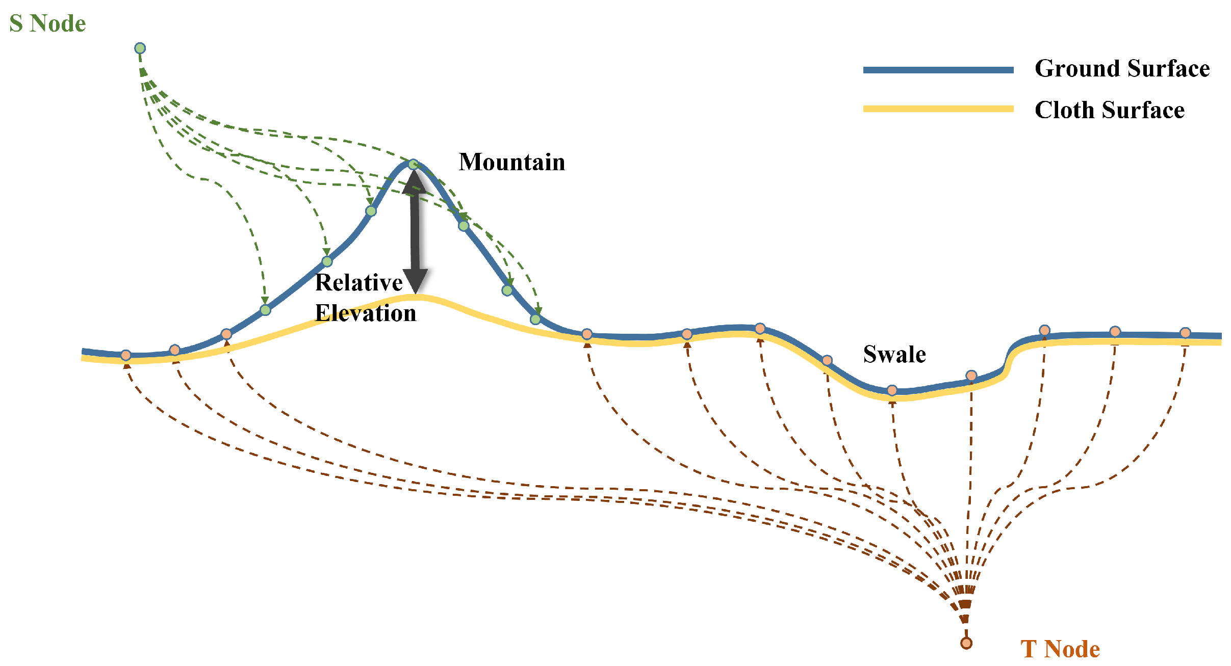
  • A certain relative elevation: a relatively noticeable elevation difference between the mountain and surrounding non-mountainous regions.
  • A certain slope: the transition region between the mountain and non-mountains should have a more obvious slope than flat regions.
  • A certain area: the mountain region should be an irregular closed polygon with a large area.
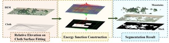
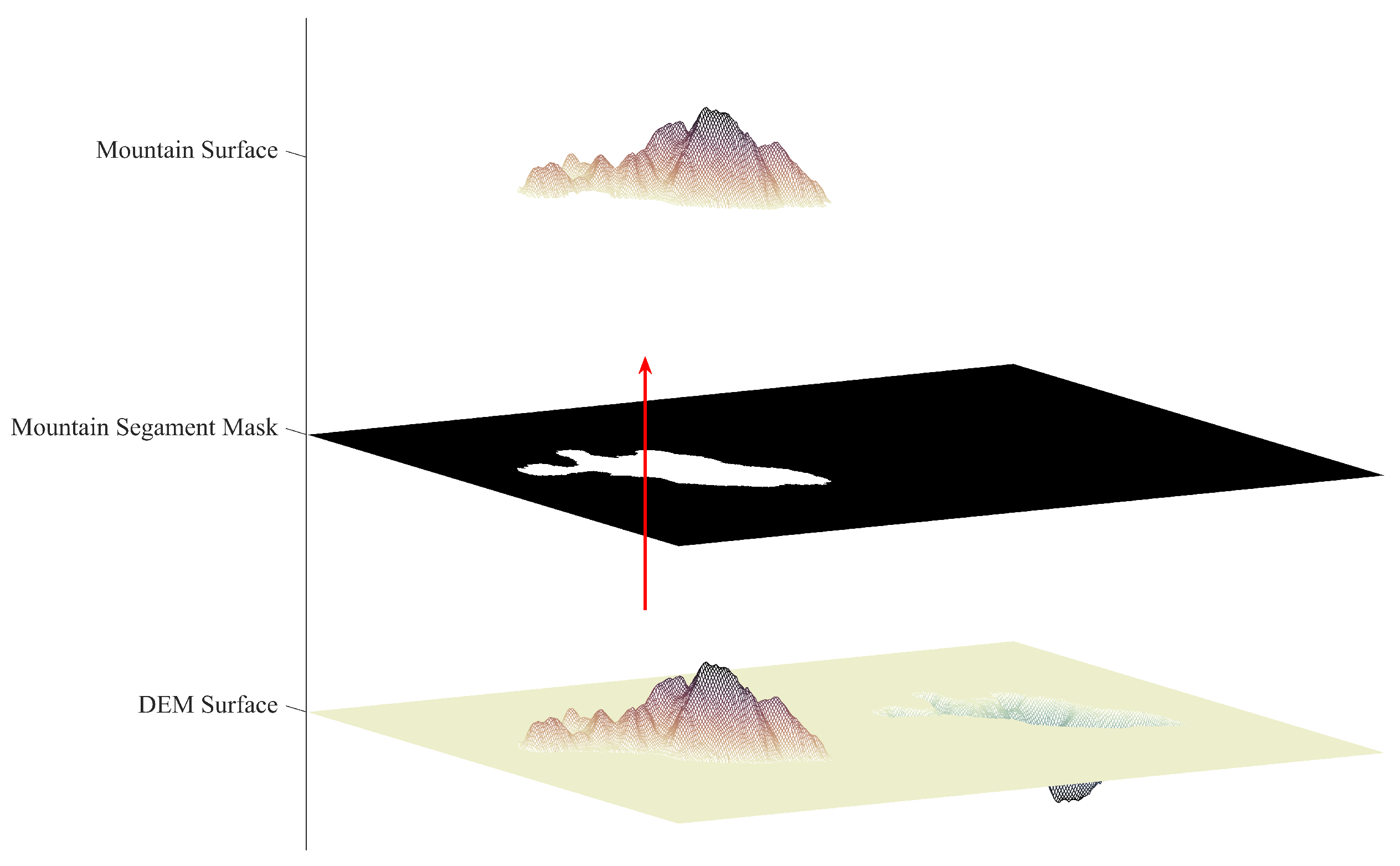
The literature [6] points out that surface morphology can be divided into seven landform types: plains, terraces, hills, small rolling hills, medium rolling hills, large rolling hills, and huge rolling hills. The method proposed in this paper aims to extract the four basic morphological landforms: small rolling hills, medium rolling hills, large rolling hills, and huge rolling hills.
However, the absolute elevation and slope of the region alone cannot effectively define the mountain, especially in the regions of plateaus with high absolute elevations and swales with sharp gradients. Therefore, further effective extraction of the surface near the mountain is needed to obtain the relative elevation of the mountain. According to the above analysis, this paper uses the cloth simulation filter (CSF) algorithm [35] to extract the surfaces which can effectively fit the flats and the swales with low gradients through a physical simulation model of a cloth (as shown in Figure 1, the cloth effectively fits in the swales and the plains and it is far away from the mountain’s surface).
In addition, the mountain region also has a certain slope and area. Although the noise in DEM data will produce a large slope, it does not have a large area. Therefore, we need to use the overall global constraint of DEMs. Since the imported digital elevation model is likely to have more than one mountain, we need to be able to detect and segment each mountain independently.
In general, combined with mountain features and the mountain distribution in a DEM, the mountain segmentation algorithm should meet the following requirements: (1) make full use of landform slopes, (2) extract and utilize the relative elevation of the landform, (3) effectively suppress the impact of noise, and (4) extract multiple mountains in a single DEM adaptively.
Given the above requirements, this paper establishes an energy function consisting of the smoothness term, the regional term, and the graph structure. By transforming the mountain extraction problem into the labeling problem of grid nodes, the final solution is obtained by minimizing the energy function through the graph cut algorithm [10,11,12]. Initially, all grid nodes in the topography are interconnected with each other and connected to both the source node (S) and the sink node (T) with weighted edges, which forms the structure of the energy function graph. By minimizing the energy function, the problem is transformed into a minimum cut/maximum flow problem of the graph. In the resulting graph, as illustrated in Figure 1, the source and sink nodes are completely disconnected. Consequently, the nodes connected to the source node are labeled as mountains, while those connected to the sink node are labeled as non-mountainous regions (i.e., flats and swales). A more detailed explanation of this process will be provided in Section 4.2 of the paper.

4. Methodology

The proposed method is divided into two parts: the computation of relative elevation based on cloth surface fitting and mountain extraction with the optimization of an energy function.
In order to effectively extract the relative elevation of the mountain, the cloth filtering algorithm is used to extract the cloth node from the existing DEM to generate the cloth surfaces. Specifically, SRTM data from NASA (https://earthexplorer.usgs.gov/ accessed on 30 September 2022) and lunar DTM data from JAXA image archive (https://darts.isas.jaxa.jp/planet/pdap/selene/index.html.en accessed on 16 October 2022) are utilized in this study. In order to make the cloth higher than the swale region and fit to the flat region as much as possible, the surface of the cloth is further processed by mean filtering, and the processed result is then defined as the ground fitting surface. Finally, the relative elevation grid can be obtained by subtracting the DEM grid from the ground fitting surface grid.
The second part of the method is constructing and minimizing the energy function, which aims to extract continuous and smooth mountain regions through the interaction between slope and relative elevation. In order to avoid the excessive influence of noise on the results, it is necessary to make a special normalization of the slope grid and then use the relative elevation grid and the special normalized grid to construct the regional term of the energy function. On the other hand, to enhance the continuity and smoothness of the region, it is necessary to use a special normalized grid to construct the smoothness term of the energy function with the basic assumption that grids with similar slopes should have similar labels. Finally, the graph cut algorithm [10,11,12] optimizes the energy function. The labels of the optimized nodes, i.e., the mountain regions and the non-mountainous regions, are taken out, as shown in Figure 2.

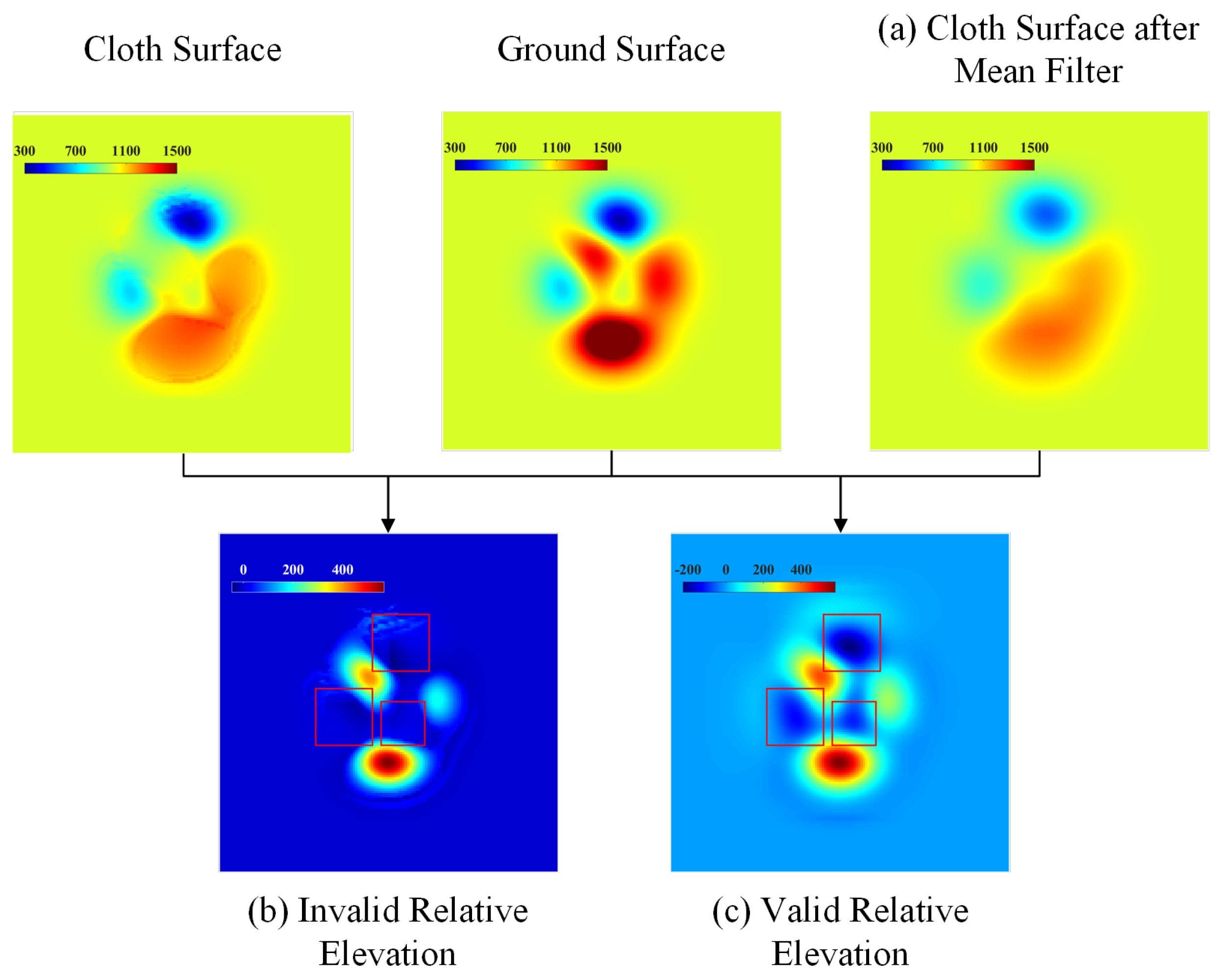
4.1. Computation of Relative Elevation Based on Cloth Surface Fitting

The relative elevations of the mountain are the key data that need to be obtained first. The traditional mean, standard deviation processing [1], and threshold method [8,9] are unable to segment multiple mountains in a wide range precisely. Therefore, the cloth is used to extract the relative elevation, on the one hand, to increase the data basis of mountain extraction, and on the other hand, to reduce the misclassification of swales.
The cloth simulation filter (CSF) algorithm is a point cloud filtering method that separates LiDAR ground points and non-ground points [35], which has the advantages of fewer parameters and a high efficiency [36]. Generally, the cloth shape generated by the simulation is used as the ground. The cloth filtering algorithm connects many cloth nodes to form a grid called a mass–spring model [37]. The nodes are subjected to stresses between points, forces from the landform surface, and gravity. Initially, the cloth nodes and point clouds are flipped [35]. Then, the cloth will start falling from the highest point until the maximum iterations or the movements reach a predefined threshold. After completing the above steps, the cloth nodes and the point clouds are flipped and restored.
In this paper, we need to extract the relative elevation of the mountain and avoid the incorrect segmentation of swales. Cloth generated by the CSF algorithm can effectively fit the surfaces of plains and swales but stay away from mountains due to the cloth hardness constraint. On this basis, the fitted cloth surface can effectively separate the mountain from the flats and the swales. Firstly, we need to initialize the DEM raster data, such as Figure 3a, and convert them to point clouds ( X , Y , H ) , where ( X , Y ) are the ground plane coordinates and H is the elevation coordinate. Then, the point clouds are flipped and the cloth nodes are initialized at the highest point, as shown in Figure 3b. Under combination effects of the gravity, the stress between the cloth nodes, and the external force from the surface, the cloth nodes iteratively stabilize with different displacements, as shown in Figure 3c. Eventually, the landform point cloud ( X , Y , H ) and the corresponding cloth nodes ( X C l o t h , Y C l o t h , Z C l o t h ) are flipped, as shown in Figure 3d. The spatial resolutions of the cloth nodes ( X C l o t h , Y C l o t h , Z C l o t h ) are much lower than those of the DEM data. Therefore, it is necessary to upsample the cloth nodes to the same resolution as the DEM data and then generate the final cloth surface, as shown in Figure 3e.
However, the function of the cloth constraint is not only to improve the mountain separability but also to reduce the probability of misclassification of swales as mountains. When the cloth surface is directly subtracted from the ground surface, the relative elevation is almost all greater than 0, and swales and flats cannot be distinguished, as shown in the red box of Figure 4b. However, the swales have a certain slope, which will still lead to misclassifying the swales as mountains. The mean filter is an efficient and simple method that can lift the dented part of the cloth. In order to reduce the above situation, it is necessary to use mean filtering to lift the cloth surface above the swales so that the algorithm can distinguish swales and flats. Therefore, the cloth surface can be used as an effective datum surface after modification, as shown in Figure 4a. Then, we use the ground surface to subtract the cloth surface. The relative elevation of the mountain is positive, and the relative elevation of the swales is negative, as shown in the red box of Figure 4c. In the subsequent segmentation process, negative regions will be strongly suppressed to avoid the swales being misclassified as mountains.
The ground fitting surface H G f s is obtained by the mean filtering algorithm, as shown in Figure 3f:
H G f s = avefliter ( H C l o t h )
Then, the relative elevation d H can be calculated by the ground fitting surface H G f s and the ground surface H, as shown in Figure 3h:
d H = H H G f s
In practice, the shape of the mountains and swales will be more complicated, as shown in the example in Figure 5, where the mountain is located at 22.4 ° N, 113.8 ° E in Figure 5a, and the simulated swale is generated by copying and reversing the mountain, as shown in Figure 5b. Then, the relative elevation is calculated by the above steps, as shown in Figure 5c,d.

4.2. Construction of Energy Function

The cloth filtering algorithm can distinguish mountain regions and non-mountain regions to a certain extent. However, due to the complexity of landforms and noise in DEMs, the cloth constraint is not enough for the high-accuracy extraction of mountain regions.
The requirement for mountain segmentation is to be as smooth and complete as possible. Therefore, the energy function is used to optimize and segment the mountain, effectively improving the smoothness and integrity of the results [38]. We set the regional features (the relative elevation and slope) and the smoothness features (the slope difference) as the terms of the energy function with regional term R ( L ) and smoothness term B ( L ) , respectively. The retentions of smoothness and regional features between raster regions are contradictory. For example, the noise will make the slope of this region larger. However, it will have a big difference from its neighbors. Therefore, if the algorithm is based only on the regional term, the region will be misjudged; if the smoothness term is introduced, the noise region may be consistent with the segmentation result of its neighbors.
We take the optimization problem above and transform it into a global energy function E ( L ) to minimize the computational problem:
min E ( L ) = λ · R ( L ) + B ( L )
where L denotes the set of labels corresponding to all raster regions: mountain (“mnt”) and background (“bkg”). E ( L ) denotes the objective function value of the global energy function. R L = p P R p L p , B L = p , q N B p , q · δ L p , L q , p denotes any pixel in the region, P denotes the set of pixels in the region, q denotes the neighboring pixels of p, and R p ( L p ) denotes the cost of pixel p corresponds to the label L. B p , q denotes the cost based on the weight of p and q calculated from the slope difference. Generally, the smaller the slope difference, the larger the weight. Coefficient λ represents the relative importance between the regional term R ( L ) and the smoothness term B ( L ) .

4.2.1. Regional Term Design

The regional term R ( L ) is the sum of the cost when pixels are designated as labels L, i.e., R ( L ) = p P R p L p , and the design of cost is related to the relative elevation d H and slope G. When a pixel is designated as the mountain, the corresponding cost is:
R p ( mnt ) = P d H mnt · P G + w H
When a pixel is designated as the background (non-mountainous region), the corresponding cost is:
R p ( bkg ) = P d H bkg · 1 P G + w H
where P G is the special normalized slope, P d H L p is the relative elevation cost factor corresponding to different labels, and w H is the weight of the relative elevation with a range between 0.3 and 0.7. When w H is larger, the slope effect is more negligible.
Slope G takes the number of degrees for representation, and the formula [39] is:
G = arctan H x 2 + H y 2
where H x and H y are the elevation gradients in the x , y direction of the gradient.
In order to suppress the noise and to create a suitable range of regional terms, the above G needs to be specially normalized to P G :
P G = 1 , G G 0 > 1 0 , G G 0 < 0 G G 0 , otherwise
where G 0 is the slope of the normalization factor. According to the table of basic terrestrial landform types proposed in the literature [6], regions with slopes greater than 5 ° are considered as mountains. It is reasonable to set the slope normalization factor G 0 to 10 ° . In other words, when G > 0.5 G 0 , the possibility of “mnt” is greater.
According to Section 4.1, in order to enhance the ability of the algorithm to segment mountains, the relative elevation d H is used to calculate the cost coefficients P d H mnt and P d H bkg . P d H mnt is used to increase the cost of the mountain label, and P d H bkg is used to increase the cost of the background (non-mountain) label.
The cost factor P d H mnt is defined as:
P d H mnt = 0 , 0 d H < 1 log 10 d H , d H 1
The cost factor P d H bkg is defined as:
P d H bkg = 1 , 0 > d H > e ln ( d H ) , d H e
Although the ground fitting surface is generally not higher than the ground surface, there is a small probability of producing d H < 0 only when the regions are pits or swales and the relative elevation of most plains is greater than 0 but close to 0 (it should be 0 under ideal conditions). In order to ensure that the basic cost exists in the plains and increase the cost of the swales, the cost factor of the background is set with a larger starting point and a larger growth rate. That is, the minimum value of the cost factor of the background (including the flats and the swales) is 1, and the growth function is ln ( d H ) . Mountains generally have a large relative elevation. In order to reduce the misclassification of the flats, the cost factor of the background is set with a larger starting point and a larger growth rate. That is, the minimum value of the cost factor of the mountain is 0 and the growth function is log 10 d H .

4.2.2. Smoothness Term Design

The smoothness term B ( L ) is used to increase the relevance between pixels, remove noise in the results, and smooth the segmented mountain regions or non-mountain regions. The smoothness term is defined as
B ( L ) = { p , q } N B p , q δ L p , L q
where B p , q is used to weight the discontinuity between pixels p and q. δ L p , L q indicates whether L p is equal to L q . B p , q is implied when p and q are labeled differently, so δ L p , L q is defined as
δ L p , L q = 1 , if L p L q 0 , if L p = L q
For neighboring pixels with approximate slopes, a higher cost is applied when their labels are different. It is defined as:
B p , q = exp P G p P G q 2 σ 2 · 1 dist p , q
where P G p and P G q correspond to the normalized slope of pixel p , q and d i s t p , q is the spatial distance of the neighbor pixel p , q . According to the definition of the smoothness term in the literature [38], σ is considered as a measure of noise in the image. We define it as the standard deviation of the normalized slope:
σ = i = 1 n P G μ P G n
where n is the number of the pixels and μ P G is the average of the normalized slope.

4.2.3. Energy Function Minimization

The DEM has been converted into nodes and, together with the two source nodes, forms a node set V. The nodes are connected using lines E with weights, forming the graph G = ( V , E ) [40]. The mountain region source node T and the non-mountain region source node S are separate source nodes that connect all pixel nodes.
There are two types of non-directional edges E: n-links and t-links. Each n-link connects neighboring nodes { p , q } by eight adjacencies and each t-link connects a node p to the source nodes S and T, which are constructed as two node sets { p , S } and { p , T } . The weights of each edge are defined as follows.
The weights of the n-links are:
w { p , q } = B p , q
The weights of the t-links are:
w { p , S } = λ R p ( mnt ) w { p , T } = λ R p ( obj )
where λ is often treated as a hyperparameter and represents the relative importance between the regional term R ( L ) and the smoothness term B ( L ) ; the selection of λ depends on an experimental parameter analysis (see Section 5.2.2).
According to the definition of λ , the larger λ is, the greater the weight of the smoothness term, the more resistant the method is to noise, and the smoother the segmentation result, but it is more likely to produce false connections of similar regions. The smaller λ is, the smaller the weight of the smoothness term and thus the clearer the contour of the region will be, and the method is more sensitive to small mountains and non-mountain regions but at the same time more susceptible to the influence of noise and small landform undulations.
Finally, the graph cut algorithm [10,11,12] is used to cut off part of the connection edge, and the mountain region source node and non-mountain region source node are completely separated. That is, the energy function is minimized. The pixel connected to the mountain source node T corresponds to the mountain region. The pixel connected to the non-mountain source node S corresponds to the non-mountain region, so all the pixels are labeled and each pixel is assigned as 0, 1 shown in Figure 6.

5. Experiment and Analysis

5.1. Data and Research Area

In order to verify the effectiveness of the proposed method, it was tested on four referenced DEM datasets from SRTM collected by NASA and one DSM dataset referenced from the JAXA image archive. This includes parts of Guangdong Province in southeastern China (22 ° ∼23 ° N, 113 ° ∼114 ° E, Dataset I), Jiangxi Province, China (26 ° ∼27 ° N, 115 ° ∼116 ° E, Dataset II), Nevada, USA (39 ° ∼40 ° N, 117 ° ∼116 ° W, Dataset III), California, USA (34 ° ∼35 ° N, 118 ° ∼117 ° W, Dataset IV), and the lunar Montsenogradov Mountains ( 21 ° ∼24 ° N, 33 ° ∼30 ° W, Dataset V). Figure 7a–e shows the elevation and mountain shading for datasets I~V, where red indicates a higher elevation and blue shows a lower elevation.
In order to evaluate the mountain segmentation results, this paper manually drew mountain masks for datasets I~V, as shown in Figure 7f–j. These mountain masks were taken as true values to evaluate the accuracy of the mountain segmentation results.

5.2. Accuracy Analysis

This paper tested the proposed method on the above five datasets to extract mountain regions with high relative elevations and slopes. In order to comprehensively evaluate the performance of the proposed method, this paper adopted five different accuracy metrics, e.g., precision, recall, overall accuracy (OA), intersection over union (IoU), and F1 score. This paper then found the optimal parameters of the proposed method using dataset I and dataset V by gradually changing the parameters and determining those with the highest accuracy. The optimal parameters were finally fixed in all datasets, and the proposed method was compared with other state-of-the-art methods.

5.2.1. Precision Analysis Index

In order to evaluate the performance of the proposed method, some accuracy metrics (e.g., precision, recall, overall accuracy (OA), intersection of union (IoU), and F1) were used for both the proposed method and other state-of-the-art methods.
We first compared the mountain segmentation results with the true values. We counted the number of true positive sample pixels T P , the number of true negative sample pixels T N , the number of false positive sample pixels F P , and the number of false negative sample pixels F N . Based on this, the following five metrics were derived.
Precision = T P T P + F P Recall = T P T P + F N OA = T P + T N T P + F P + T N + F N IoU = area ( A B ) area ( A B ) F 1 = 2 Precision Recall Precision + Recall

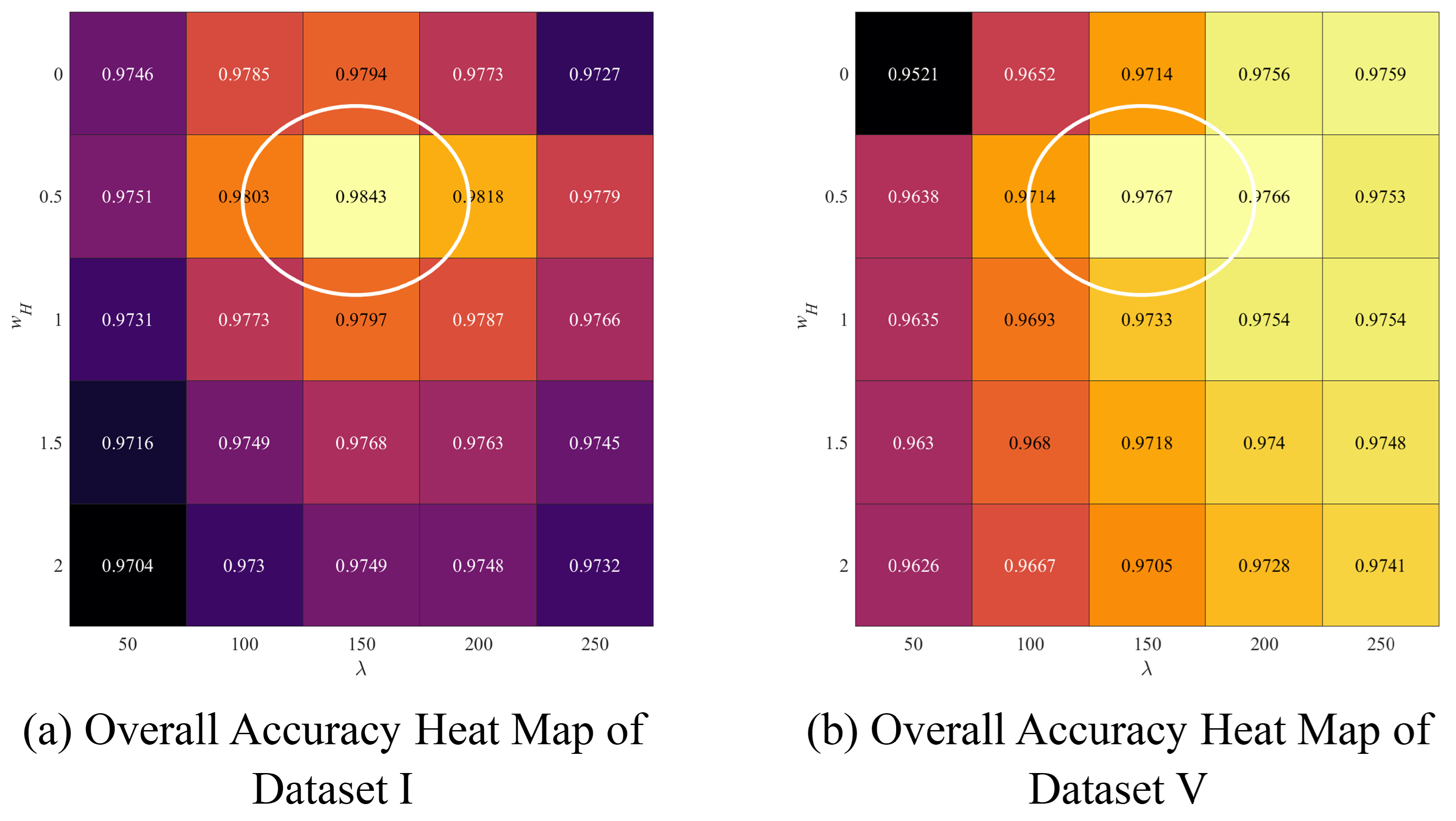
5.2.2. Optimal Parameter Adjustment

The proposed method realizes mountain segmentation by minimizing the energy function, where several important parameters need to be manually adjusted, including the coefficient λ and the weight of relative elevation w H in Equations (3)–(5). The coefficient λ maintains the smoothness of the results and reduces the influence of noise. The weight w H is used to increase the contribution of the relative elevation in the optimization, which plays an important role in removing pits or swales. This paper adopted the variable control method and a visual analysis to determine the most optimal choice of the parameters.
In this paper, dataset I and dataset V were selected for parameter adjustment. The region noise and small fluctuations in dataset I are more distributed, and dataset V has a large distribution of craters. The experimental interval of the parameter λ was mainly based on the proportional relationship between the smoothness and regional terms. The corresponding segmentation results were obtained when λ was set within the interval of [ 50 , 250 ] . The relative elevation weight w H represents the contributions of the relative elevation in the optimization. In order to make the effects of relative elevation and normalized slope similar, it was reasonable to set the relative elevation weight range from 0 to 2. In order to select reasonable parameters, we analyzed the segmentation results of λ at 50, 100, 150, 200, and 250 with a step of 50 and w H at 0 , 0.5 , 1 , 1.5 , and 2 with a step of 0.5.
Figure 8 shows the heat map of the overall accuracy of dataset I and dataset V, where a high value means a high accuracy. Through 25 groups of segmentation results with different λ and w H , it was found that the highest accuracy can be obtained when the parameters are λ = 150 and w H = 0.5 .
In addition to the heat map of overall accuracy, a more detailed analysis of different parameters was carried out by checking the corresponding segmentation results in some difficult regions, as shown in Figure 9 and Figure 10.
Figure 9 shows the results of dataset I at λ = 150 and w H = 0.5 , λ = 100 and w H = 0.5 , and λ = 200 and w H = 0.5 , where the first row represents the region in the red bounding box, and the second row represents the region in the yellow bounding box. The parameter λ determines the contributions of the smoothness term in the optimization. A higher λ will generate a strong smoothness constraint and vice versa. If λ is too high, some small mountains may be filtered away, as shown in the green box of Figure 9e at λ 250 . However, if λ is too low, some noise in the DEM cannot be removed, as shown in the blue box of Figure 9h at λ 50 . Therefore, an appropriate choice of λ is necessary for high-accuracy mountain segmentation, i.e., λ = 150 .
On the other hand, Figure 10 shows the results of dataset V at λ = 150 and w H = 0.5 , λ = 150 and w H = 0 , and λ = 150 and w H = 1 , where the first row represents the region in the red bounding box, and the second row represents the region in the yellow bounding box. The parameter w H determines the contributions of the relative elevation in the optimization. A higher w H will generate a strong cloth constraint and vice versa. If w H is too high, some regions with large relative elevations and small slopes may be misclassified as mountains, as shown in the green box of Figure 10e at w H 1 . However, if w H is too low, some pits with a large slope will be mistakenly classified as a mountain, as shown in the blue box of Figure 10h at w H = 0 . Therefore, an appropriate choice of w H is necessary for high-accuracy mountain segmentation, i.e., w H = 0.5 .
We conducted an experimental analysis of different parameters. We determined the optimal combination of parameters as λ = 150 and w H = 0.5 via a visual analysis and overall accuracy heat maps of dataset I and V. The combination of parameters was fixed for the following comparison and analysis.

5.2.3. Algorithm Comparison and Analysis

In this paper, the results of the proposed method were compared with the lunar mountain detection method (MDA) [3], the landform mask method (SNAP) in SNAP™ (https://earth.esa.int/eogateway/tools/snap) from the European Space Agency, and the multi-scale segmentation method (Eco) in eCognition™ [1] (https://geospatial.trimble.com/products-and-solutions/trimble-ecognition) from Definiens Imaging. The proposed method and the MDA method were implemented using MATLAB R2022b, while SNAP and Eco were implemented using the aforementioned software. The MDA method segments the mountains by converting the DEM data into image entropy and using the Riley entropy threshold to calculate the mask of mountains; the SNAP method uses a certain size window to calculate the slope in the DEM and then segments mountains by a threshold constraint, which will decrease the resolution of the DEM; and finally, the Eco method divides the landform into eight types of objects by multi-scale segmentation based on the elevation and uses standard deviation of the object mean value to achieve segmentation of the features [1].
This paper compared the proposed method with the above methods on datasets I∼V and comprehensively evaluated their performance by utilizing the five accuracy metrics. The different datasets represent different typical landforms. For example, dataset I corresponds to regions with more plains and fewer mountains; dataset II corresponds to regions with more mountains and fewer plains; dataset III corresponds to regions with more complex mountain bases; dataset IV corresponds to regions with more small mountains; and dataset V corresponds to regions with lunar craters. The mountain segmentation accuracy of different methods is shown in Table 1.
Table 1 shows the segmentation accuracy of each method on each dataset, where the overall accuracy of the proposed method reaches more than 90 % for all datasets. The proposed method produces better results and can more stable segmentation against various landforms.
In order to evaluate the overall performance of each method, we averaged the results of each accuracy metric across all datasets. The average accuracy of each method is shown in Figure 11. Compared with other methods, the proposed method achieved the highest segmentation accuracy with the highest average precision, OA, IoU, and F1.
However, since the recall is used to assess mountain coverage, the recall of the proposed method did not reach the maximum value. SNAP and MDA have relatively high coverage of results, i.e., a high TP, because the methods are based on entropy or slope and are extremely sensitive to the results of the DEM. Although the results of SNAP and MDA could cover many mountains leading to a high recall, noise and swale misjudgment were also introduced. At the same time, the proposed method could deal with the above problems with better performance and had a lower misclassification probability.
In order to analyze the performance more comprehensively, the results of all methods are visualized for comparison. By comparing the segmentation results of each method with the manual mountain masks, the differences are shown in different colors in Figure 12a–e, where red indicates the FN region, yellow indicates the FP region, and cyan indicates the TN region, while the TP region is shown directly as mountain shading.
According to Figure 12, the results of the proposed method are generally better than others. For example, in dataset I, II, and IV, the proposed method generated the smoothest and most complete mountains among all the methods. In dataset III, the proposed method produced the most precise mountain edges. In dataset V, the proposed method avoided misclassifying the crater bottom. The above points will also be reflected in the following detailed analysis.
In order to show the details more clearly, we focus on the misclassification and omission of the proposed method and MDA, compared with the manual mountain masks. As the overall accuracies of SNAP and Eco are lower than MDA, both SNAP and Eco were not considered in the visual comparisons of the local zoomed-in regions. In addition, SNAP and MDA are both methods based on roughness. Therefore, we only consider MDA and the proposed method for a detailed comparison.
Before the detailed analysis, we first discuss the characteristics of all the methods and the corresponding segmentation results:
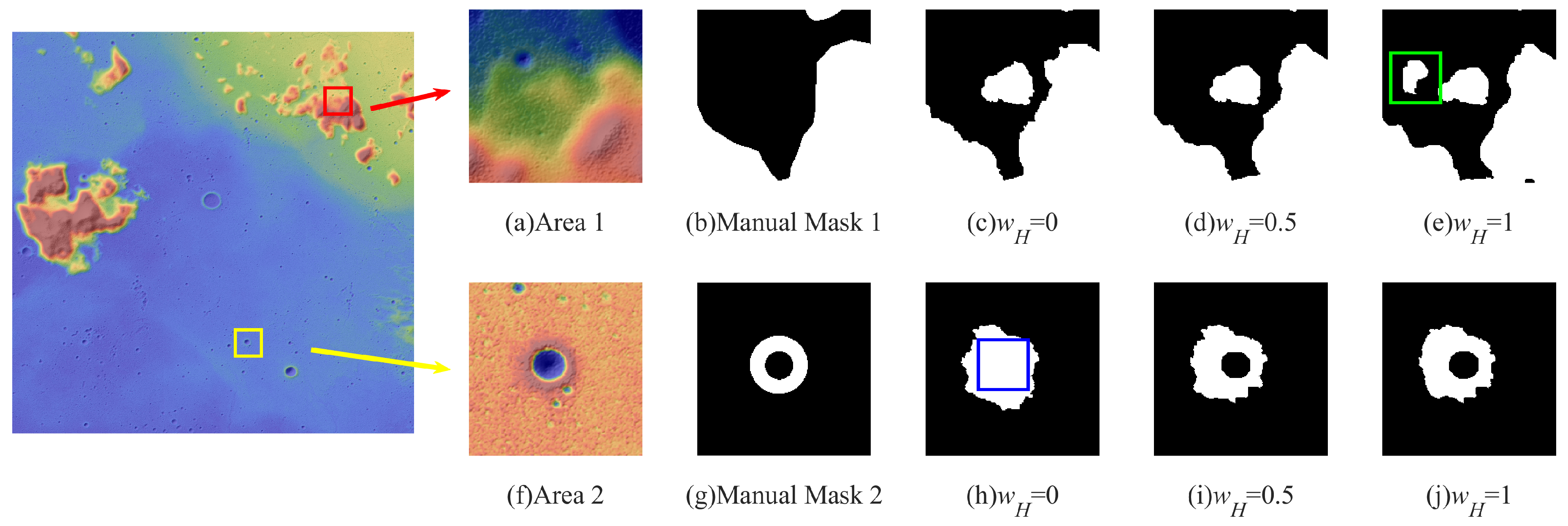
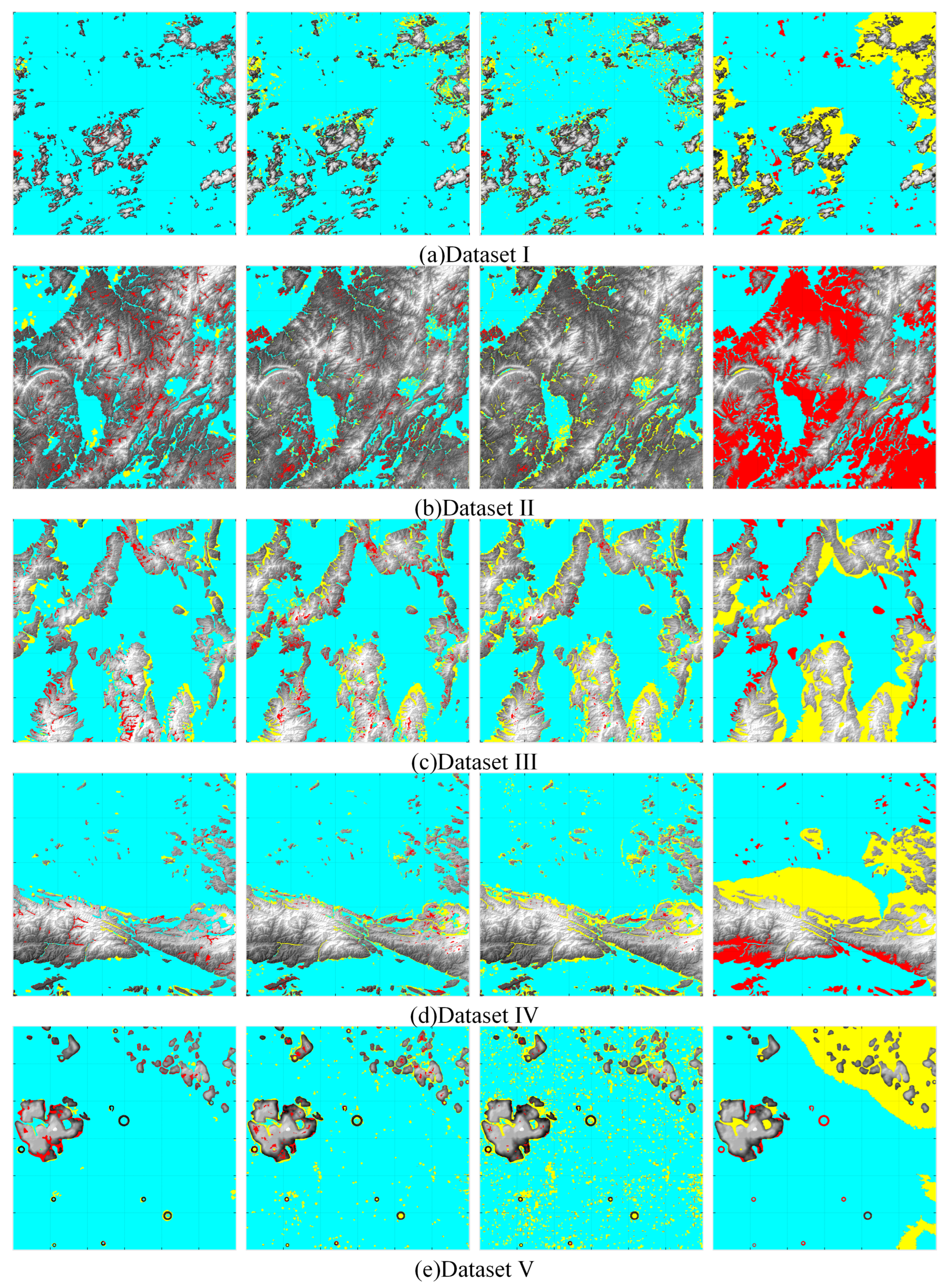
  • The proposed method effectively reduced the noise, and the mountain results were more complete and smoother in each dataset through the smoothness term constraint in the energy function, as shown in Figure 12a–e. This method optimized the global energy function in the pixels as the unit to realize the segmentation of fine mountains, and better results can be seen in Figure 12c. It introduced relative elevation, so false segmentation could be effectively avoided for lunar craters, as shown in Figure 12e;
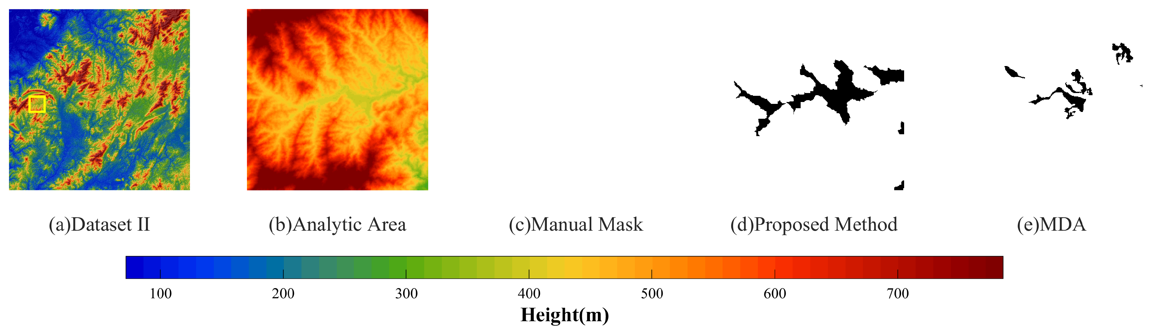
  • MDA is a mountain segmentation method that uses wavelet de-noising pretreatment. Wavelet de-noising can reduce the impact of noise to a certain extent; however, this inevitably affected the image resolution and it was unable to achieve fine segmentation, especially for the edge of the mountain, see Figure 12c. In addition, MDA is a method to calculate entropy based on a sliding window. Therefore, large fluctuations or noise in the sliding window can directly affect the entropy of the nearby region, resulting in false segmentation of the whole block. Therefore, this method was also extremely sensitive to noise, as shown in Figure 12a,c,d. This method only segments mountains based on roughness, so it could not distinguish swales or pits, resulting in many false segmentations of swales or mountains, Figure 12d,e. In addition, MDA is a local method based only on the pixels and their neighborhood. Therefore, for regions where their entropies were near the threshold, fragmented segmentation results were often produced and the mountain was not presented completely, see Figure 12a,d;
  • SNAP is a method to extract the slope in a fixed window by a threshold value based on the calculation of the slope in a fixed window. It has similar characteristics to MDA, which is also sensitive to noise, will reduce the data resolution, and cannot judge swales and pits;
  • Eco is an object-oriented mountain segmentation method. Firstly, multi-scale segmentation of eCognition is used to classify each region, and then objects are selected as mountain regions based on the thresholds of the object mean and standard deviation. However, the selection of objects by the threshold method often fails to adapt to all mountains and different types of landforms, which inevitably leads to the misclassification of most flat land or mountains. Therefore, this method is only suitable for landform statistics in most regions.
Next, this paper discusses and verifies the above analysis in detail based on Figure 12, Figure 13, Figure 14, Figure 15, Figure 16, Figure 17 and Figure 18.
The region corresponding to dataset I mainly consists of a few mountains and mostly plains. There is a clear segmentation boundary between mountains and plains, while the noise and the undulations of the ground increase the classification difficulty.
Figure 12a shows the segmentation results of dataset I. The proposed method produced the smoothest results with the least noise. MDA and SNAP methods produced the most misclassification results due to the increased noise and relief distributed in the whole picture. These local methods are based on entropy or slope and are more susceptible to noise and the relief of landforms, resulting in false segmentation.
As shown in Figure 13, the proposed method could effectively perform segmentation in this region. At the same time, MDA produced misclassification based on only roughness.
The region corresponding to dataset II mainly consists of mountains and a few plains, and the mountains are interspersed with plains. The interlacing of mountains (including valleys and ridges) and plains in dataset II increases the classification difficulty.
Figure 12b shows the segmentation results of dataset II. The proposed, MDA, and SNAP methods all achieved good results. The accuracies of the three methods decreased to a certain extent due to the presence of valleys, but it had the greatest impact on the proposed method. Due to the inaccurate elevation threshold of Eco, large mountain regions were misclassified.
The overall accuracies of the proposed method, MDA, and SNAP, were more than 90% and similar to each other, but Eco produced a relatively large error. However, the overall accuracy of the proposed method was higher than that of MDA.
The proposed method misclassified some valleys, while the MDA method was more sensitive to topographic relief. It uses window entropy calculations; thus, gradient changes have a larger impact range covering the entire window region, hence resulting in a lower omission rate.
As shown in Figure 15, the valley in Figure 15b is relatively flat but still belongs to the mountain. The proposed method and MDA produced misclassifications, with a smaller misclassification through MDA, leading to a slightly lower overall accuracy than the proposed method.
The misclassification observed in this specific region can be attributed to several factors. Firstly, the region itself lacks significant variations in elevation, resulting in a relatively uniform appearance. Then, its location in the central part of the mountain contributes to the minimal relative elevation from the cloth surface. Consequently, the cloth constraint fails to provide effective assistance in this particular case, as illustrated in Figure 14.
The region corresponding to dataset III includes mountains and plains which are relatively uniformly distributed. The mountains are striped with complex foothill lines distributed and contracted inside and outside, except for undulations near the foothills. The complex shape of the foothills makes the segmentation more difficult.
Figure 12c shows the segmentation results of dataset III. The proposed method was the most accurate for the treatment of complex foothills. However, SNAP and MDA methods calculate the entropy or slope in the window, so they introduced the influence of the surrounding large gradient change pixels, resulting in the region near the mountain baselines no longer being segmented.
As shown in Figure 16, the proposed method could deal with the contraction of the inner and outer foothills, and the result was consistent with the manual mask, while the MDA was segmented along the outer side.
The region corresponding to dataset IV has a rising elevation trend from low latitude to high latitude, and there are many fine-grained mountains and a small number of swales. The fine-grained mountains, rough ground, and swales make the segmentation more difficult.
Figure 12d shows the segmentation results of dataset IV. The proposed method was able to deal with small sheet mountain ranges. In addition, the method was almost unaffected by elevation trends due to the introduction of relative elevation, and thus produced reliable results. On the contrary, MDA and SNAP were more sensitive to subtle relief and noise due to the change in elevation. The elevation changes led to an overall increase in the slope of the plains, and there was also influence from noise. MDA and SNAP inevitably produced fragmentation of the mountain, reducing the integrity and smoothness of the results.
As shown in Figure 17, the proposed method could effectively deal with the elevation trend, the undulations, fine-grained mountains, and swales. At the same time, MDA inevitably misclassified the swales and undulations.
The region corresponding to dataset V has many craters and lunar mountains. The lunar craters increase the difficulty of segmentation.
Figure 12e shows the segmentation results of dataset V. The proposed method could distinguish the craters from the mountains due to the introduction of relative elevation. In contrast, MDA and SNAP segmented mountains only based on slope and entropy and could not distinguish craters and mountains with large slopes, so many lunar craters were misclassified as mountains.
As shown in Figure 18, the proposed method could offset the effect of the slope of lunar craters and correctly classify most craters as non-mountainous regions. In contrast, MDA misclassified the craters because they also had relative slopes.
The proposed method can effectively deal with pits, complex foothills, noise, and ground undulations according to the above results. At the same time, MDA and SNAP segment mountains based only on the roughness and slope and need to use a large window to calculate the entropy and slope, which introduces the influence of all the pixels in the window and is susceptible to noise. Eco is based on the elevation mean and standard deviation, which is suitable for the statistics of large regions but is ineffective for finely segmented mountains.
The F1 and IoU values obtained by the proposed method are the highest in each sample among all methods. These two indexes describe the comprehensive indexes of recall and precision. In other words, the proposed method has the best all-around performance.

6. Conclusions

Mountain segmentation is an important task in the fields of geology and surveying. However, most existing methods often face limitations due to the complexity of mountain features. In order to design a more flexible, lightweight, and effective method, this paper proposes a mountain segmentation method based on global optimization with a cloth simulation constraint.
The contribution of the method is to formulate the mountain extraction problem as an optimal solution of a global energy function, which is then optimized by the graph cut algorithm. Generally, the energy function comprises two parts: the regional term and the smoothness term. Considering the distinction between mountains and plains, the design of the regional term is mainly based on the relative elevation and the slope, where the relative elevation is derived from the elevation difference between the elevation value of the simulated cloth surface and the ground elevation model. On the other hand, the design of the smoothness term is based on the principle that a pixel with a similar slope has a high probability of belonging to the same feature type. Compared with other methods, the proposed method can reduce the interference of complex landforms and noise, effectively extract mountain regions in a complex landform environment (including pits or swales), and produce the most precise mountain edges.
To validate the correctness and effectiveness of the method, four SRTM DEM datasets and one lunar DSM dataset were utilized. The experimental results demonstrate that the proposed method achieves a significantly higher accuracy compared to three cutting-edge methods based solely on roughness or elevation. It effectively maintains the accuracy and smoothness of mountain boundaries while avoiding misclassification of craters, swales, and small undulating regions. Compared with the other three methods, the overall accuracy of the proposed method improved by 8.74% on average, with a minimum of 1.84% and a maximum of 19.45%. The F1-score improved by 14.70 on average, with a minimum of 4.79 and a maximum of 29.07. The IoU improved by 20.46 on average, with a minimum of 7.59 and a maximum of 38.94. The accuracy improved by 21.63% on average, with a minimum of 10.72% and a maximum of 33.26%.
Currently, the proposed method still has certain limitations. In terms of efficiency, although graph cut exhibits a good performance in the optimization of mountain segmentation, the efficiency of our method still needs improvement compared to traditional approaches. With the SRTM dataset, with sizes of 3600 ∗ 3600 pixels and resolutions of 1 arc-second, it takes approximately 50 s for the proposed method with a computer configuration of a single thread of an Intel(R) Core(TM) i7-10700 CPU @ 2.90 GHz. In practical applications, the computational speed can be enhanced through techniques such as parallel block processing or downsampling. Regarding segmentation boundaries, although the energy function solution produces accurate, smooth boundaries, occasional over-segmentation or under-segmentation may occur during the boundary delineation of highly complex mountain regions. The proposed cloth simulation constraint effectively avoids misclassification of crater-like features and introduces relative elevation data. However, it may also impact the delineation of mountain boundaries. It is possible that the cloth surface could extend higher than the actual terrain, leading to an excessive inward contraction of certain mountain base areas. Such an issue of the cloth surface should be improved.
In future research, efforts will be made to address the aforementioned limitations and further improve the proposed method. One area of focus will be enhancing the algorithm’s efficiency by exploring techniques such as parallel processing. Additionally, there will be a concerted effort to refine the segmentation boundaries, particularly in complex terrains. Furthermore, improvements will be made to the cloth simulation constraint, aiming to better align the resolution of the cloth surface with the terrain data. Expanding the applicability of the method to handle various landforms and investigating potential integrations with advanced machine learning techniques are also key targets for future research.

Author Contributions

Conceptualization, X.H. and L.W.; methodology, L.W. and X.H.; software, L.W. and J.H.; validation, L.W., X.H. and J.H.; formal analysis, L.W.; investigation, L.W. and J.H.; resources, X.H.; data curation, X.H.; writing—original draft preparation, L.W.; writing—review and editing, L.W., J.H. and X.H; visualization, L.W. and J.H.; supervision, X.H.; project administration, X.H.; funding acquisition, X.H. All authors have read and agreed to the published version of the manuscript.

Funding

This research was funded by the National Natural Science Foundation of China (grant number 41701540) and the Basic Startup Funding of Sun Yat-sen University (grant number 76230-18841205).

Data Availability Statement

Some of the data presented in this study are openly available. The SRTM data accessed on 30 September 2022 are available at https://earthexplorer.usgs.gov/, and the lunar orbital DSM dataset accessed on 16 October 2022 is available at https://ode.rsl.wustl.edu/moon/productsearch.

Conflicts of Interest

The authors declare no conflict of interest.

References

  1. Drăguţ, L.; Eisank, C. Automated object-based classification of topography from SRTM data. Geomorphology 2012, 141–142, 21–33. [Google Scholar] [CrossRef] [PubMed] [Green Version]
  2. Wang, D.; Laffan, S.; Liu, Y.; Wu, L. Morphometric characterisation of landform from DEMs. Int. J. Geogr. Inf. Sci. 2010, 24, 305–326. [Google Scholar] [CrossRef] [Green Version]
  3. Micheal, A.A.; Vani, K. Automatic mountain detection in lunar images using texture of DTM data. Comput. Geosci. 2015, 82, 130–138. [Google Scholar] [CrossRef]
  4. Zhou, F.; Xiao, Z. Slope distribution feature method for mountaintop extraction from grid DEM. Geomat. Inf. Sci. Wuhan Univ. 2022, 1–9. [Google Scholar] [CrossRef]
  5. Drăguţ, L.; Eisank, C. Object representations at multiple scales from digital elevation models. Geomorphology 2011, 129, 183–189. [Google Scholar] [CrossRef] [Green Version]
  6. Zhou, C.; Cheng, W. Research on the Classification System of Digital Land Gromorphology of 1:1000000 in China. J. Geo-Inf. Sci. 2009, 11, 707–724. [Google Scholar]
  7. Li, S.; Xiong, L.; Tang, G.; Strobl, J. Deep learning-based approach for landform classification from integrated data sources of digital elevation model and imagery. Geomorphology 2020, 354, 107045. [Google Scholar] [CrossRef]
  8. Hu, J.; Luo, M.-L.; Bai, L.; Duan, J.; Yu, B. An Integrated Algorithm for Extracting Terrain Feature-Point Clusters Based on DEM Data. Remote Sens. 2022, 14, 2776. [Google Scholar] [CrossRef]
  9. Luo, M.-L. Mountain peaks extraction based on geomorphology cognitive and space segmentation. Sci. Surv. Mapp. 2010, 35, 126–128. [Google Scholar]
  10. Boykov, Y.; Veksler, O.; Zabih, R. Fast approximate energy minimization via graph cuts. IEEE Trans. Pattern Anal. Mach. Intell. 2001, 23, 1222–1239. [Google Scholar] [CrossRef] [Green Version]
  11. Kolmogorov, V.; Zabin, R. What energy functions can be minimized via graph cuts? IEEE Trans. Pattern Anal. Mach. Intell. 2004, 26, 147–159. [Google Scholar] [CrossRef] [PubMed] [Green Version]
  12. Boykov, Y.; Kolmogorov, V. An experimental comparison of min-cut/max- flow algorithms for energy minimization in vision. IEEE Trans. Pattern Anal. Mach. Intell. 2004, 26, 1124–1137. [Google Scholar] [CrossRef] [PubMed] [Green Version]
  13. Wade, A.P. The Relationship between Topography and Geology. Aust. Surv. 1935, 5, 367–371. [Google Scholar] [CrossRef]
  14. Manoutsoglou, E.; Lazos, I.; Steiakakis, E.; Vafeidis, A. The Geomorphological and Geological Structure of the Samaria Gorge, Crete, Greece—Geological Models Comprehensive Review and the Link with the Geomorphological Evolution. Appl. Sci. 2022, 12, 10670. [Google Scholar] [CrossRef]
  15. Morelli, D.; Locatelli, M.; Corradi, N.; Cianfarra, P.; Crispini, L.; Federico, L.; Migeon, S. Morpho-Structural Setting of the Ligurian Sea: The Role of Structural Heritage and Neotectonic Inversion. J. Mar. Sci. Eng. 2022, 10, 1176. [Google Scholar] [CrossRef]
  16. Dikau, R.; Brabb, E.E.; Mark, R.M. Landform Classification of New Mexico by Computer. 1991. Available online: https://pubs.er.usgs.gov/publication/ofr91634 (accessed on 16 October 2022).
  17. Galli, M.; Ardizzone, F.; Cardinali, M.; Guzzetti, F.; Reichenbach, P. Comparing landslide inventory maps. Geomorphology 2008, 94, 268–289. [Google Scholar] [CrossRef]
  18. Zheng, Z.; Xiao, X.; Zhong, Z.C.; Zang, Y.; Yang, N.; Tu, J.; Li, D. A Rapid and High-Precision Mountain Vertex Extraction Method Based on Hotspot Analysis Clustering and Improved Eight-Connected Extraction Algorithms for Digital Elevation Models. Remote Sens. 2021, 13, 81. [Google Scholar] [CrossRef]
  19. Meng, X.; Xiong, L.; Yang, X.; Yang, B.; Tang, G. A terrain openness index for the extraction of karst Fenglin and Fengcong landform units from DEMs. J. Mt. Sci. 2018, 15, 752–764. [Google Scholar] [CrossRef]
  20. Heung, B.; Ho, H.C.; Zhang, J.; Knudby, A.; Bulmer, C.E.; Schmidt, M.G. An overview and comparison of machine-learning techniques for classification purposes in digital soil mapping. Geoderma 2016, 265, 62–77. [Google Scholar] [CrossRef]
  21. Minár, J.; Evans, I.S. Elementary forms for land surface segmentation: The theoretical basis of terrain analysis and geomorphological mapping. Geomorphology 2008, 95, 236–259. [Google Scholar] [CrossRef]
  22. Evans, I.S. Geomorphometry and landform mapping: What is a landform? Geomorphology 2012, 137, 94–106. [Google Scholar] [CrossRef]
  23. Song, X.D.; Brus, D.J.; Liu, F.; Li, D.C.; Zhao, Y.G.; Yang, J.L.; Zhang, G.L. Mapping soil organic carbon content by geographically weighted regression: A case study in the Heihe River Basin, China. Geoderma 2016, 261, 11–22. [Google Scholar] [CrossRef]
  24. Miliaresis, G.C.; Argialas, D.P. Segmentation of physiographic features from the global digital elevation model/GTOPO30. Comput. Geosci. 1999, 25, 715–728. [Google Scholar] [CrossRef]
  25. Saha, K.; Wells, N.A.; Munro-Stasiuk, M. An object-oriented approach to automated landform mapping: A case study of drumlins. Comput. Geosci. 2011, 37, 1324–1336. [Google Scholar] [CrossRef]
  26. Romstad, B.; Etzelmüller, B. Mean-curvature watersheds: A simple method for segmentation of a digital elevation model into terrain units. Geomorphology 2012, 139–140, 293–302. [Google Scholar] [CrossRef] [Green Version]
  27. Verhagen, P.; Drăguţ, L. Object-based landform delineation and classification from DEMs for archaeological predictive mapping. J. Archaeol. Sci. 2012, 39, 698–703. [Google Scholar] [CrossRef]
  28. Berral, J.L.; Gavaldà, R.; Torres, J. Power-Aware Multi-data Center Management Using Machine Learning. In Proceedings of the 2013 42nd International Conference on Parallel Processing, Lyon, France, 1–4 October 2013. [Google Scholar]
  29. Ehsani, A.H.; Quiel, F. Geomorphometric feature analysis using morphometric parameterization and artificial neural networks. Geomorphology 2008, 99, 1–12. [Google Scholar] [CrossRef]
  30. Leon, F.P.; Christopher, W.H.; Stephen, P.S.; Alexander, M.A. Automated detection of geological landforms on Mars using Convolutional Neural Networks. Comput. Geosci. 2017, 101, 48–56. [Google Scholar]
  31. Li, W.; Zhou, B.; Hsu, C.Y.; Li, Y.; Ren, F. Recognizing terrain features on terrestrial surface using a deep learning model. In Proceedings of the Artificial Intelligence and Deep Learning for Geographic Knowledge Discovery, Redondo Beach, CA, USA, 7 November 2016. [Google Scholar]
  32. Marcus, G. Deep Learning: A Critical Appraisal. arXiv 2018, arXiv:1801.00631. [Google Scholar]
  33. Minar, M.R.; Naher, J. Recent Advances in Deep Learning: An Overview. arXiv 2018, arXiv:1807.08169. [Google Scholar]
  34. Zhong, X.; Liu, S. Research on the Mountain Classification in China. Mt. Res. 2014, 32, 129–140. [Google Scholar]
  35. Zhang, W.; Qi, J.; Wan, P.; Wang, H.; Xie, D.; Wang, X.; Yan, G. An Easy-to-Use Airborne LiDAR Data Filtering Method Based on Cloth Simulation. Remote Sens. 2016, 8, 501. [Google Scholar] [CrossRef]
  36. Cai, S.; Zhang, W.; Qi, J.; Peng, W.; Shao, J.; Shen, A. Applicability Analysis of Cloth Simulation Filtering Algorithm for Mobile Lidar Point Cloud. In Proceedings of the ISPRS—International Archives of the Photogrammetry, Remote Sensing and Spatial Information Sciences, Beijing, China, 7–10 May 2018; Volume XLII-3, pp. 107–111. [Google Scholar] [CrossRef] [Green Version]
  37. Provot, X. Deformation Constraints in a Mass-Spring Model to Describe Rigid Cloth Behavior; Canadian Information Processing Society: Mississauga, ON, Canada, 1995. [Google Scholar]
  38. Boykov, Y.; Jolly, M.P. Interactive Graph Cuts for Optimal Boundary & Region Segmentation of Objects in N-D Images. In Proceedings of the Eighth IEEE International Conference on Computer Vision. ICCV 2001, Vancouver, BC, Canada, 7–14 July 2001; Volume 1, pp. 105–112. [Google Scholar] [CrossRef]
  39. An, T.G.; Mudan, Z. Geographic Information System; China Science Publishing & Media LTD.: Beijing, China, 2010. [Google Scholar]
  40. Guo, B.; Zuo, X. An Optimized Point Cloud Classification and Object Extraction Method Using Graph Cuts. IEEE Access 2020, 8, 188515–188525. [Google Scholar] [CrossRef]
Figure 1. Cloth simulation filter and energy function diagram: S Node is connected to pixels marked as mountains, and T Node is connected to pixels marked as non-mountains after the graph cut.
Remotesensing 15 02966 g001
Figure 2. Workflow of the proposed method.
Remotesensing 15 02966 g002
Figure 3. Workflow of the computation.
Remotesensing 15 02966 g003
Figure 4. Comparison of relative elevation extraction: (a) the cloth surface is lifted at the swales after post-processing. (b) Relative elevation of the cloth surface without post-processing vs. (c) relative elevation of the cloth surface with post-processing.
Remotesensing 15 02966 g004
Figure 5. Flow chart for relative elevation extraction using real landform data.
Remotesensing 15 02966 g005
Figure 6. DEM surface, segment mask, and final mountain segmentation results.
Remotesensing 15 02966 g006
Figure 7. Visualization of DEMs and manual mountain masks in the study area.
Remotesensing 15 02966 g007
Figure 8. Overall accuracy heat map of the parameter adjustment: The brighter the color, the higher the corresponding accuracy. The accuracy reaches its highest level, indicated by the white circle.
Remotesensing 15 02966 g008
Figure 9. Comparison of segmentation results with different parameters for dataset I.
Remotesensing 15 02966 g009
Figure 10. Comparison of segmentation results with different parameters for dataset V: The yellow and red boxes represent the selected analysis regions, while the green and blue boxes represent areas with misclassifications or omissions.
Remotesensing 15 02966 g010
Figure 11. Statistics of the indexes of each method.
Remotesensing 15 02966 g011
Figure 12. Visualization of segmentation results (from left to right corresponding to the results of the proposed method, MDA, SNAP, and Eco, respectively): The red indicates the false negative (FN) region, the yellow indicates the false positive (FP) region, and the cyan indicates the true negative (TN) region. The true positive (TP) region is directly depicted as mountain shading.
Remotesensing 15 02966 g012
Figure 13. Regional analysis of dataset I.
Remotesensing 15 02966 g013
Figure 14. Illustration of misclassified results in a valley region.
Remotesensing 15 02966 g014
Figure 15. Regional analysis of dataset II.
Remotesensing 15 02966 g015
Figure 16. Regional analysis of dataset III.
Remotesensing 15 02966 g016
Figure 17. Regional analysis of dataset IV.
Remotesensing 15 02966 g017
Figure 18. Regional analysis of dataset V.
Remotesensing 15 02966 g018
Table 1. Accuracy assessment of datasets I~V: The bold values represent the highest accuracy evaluation metrics among the methods.
MethodPrecisionRecallOAIoUF1
Dataset IProposed97.71%91.93%98.43%90.00%94.73%
MDA76.78%98.90%95.25%76.12%86.44%
SNAP71.90%94.76%93.52%69.15%81.76%
Eco47.15%88.22%83.05%44.36%61.45%
Dataset IIProposed97.56%93.29%92.95%91.97%95.82%
MDA96.90%94.76%93.55%91.16%95.38%
SNAP92.37%97.79%91.99%90.48%95.00%
Eco98.99%48.74%59.67%48.50%65.32%
Dataset IIIProposed87.71%91.04%92.53%80.75%89.35%
MDA83.29%89.55%90.23%75.91%86.31%
SNAP75.61%96.13%88.01%73.38%84.65%
Eco67.95%86.69%81.36%61.53%76.18%
Dataset IVProposed93.83%94.59%96.81%89.05%94.21%
MDA88.09%94.55%95.00%83.83%91.21%
SNAP78.06%97.96%91.89%76.81%86.88%
Eco53.93%78.75%75.73%47.08%64.02%
Dataset VProposed90.45%83.05%97.52%76.35%86.59%
MDA68.62%88.82%95.00%63.16%77.42%
SNAP44.74%96.46%88.15%44.02%61.13%
Eco32.92%91.39%81.19%31.93%48.40%
Disclaimer/Publisher’s Note: The statements, opinions and data contained in all publications are solely those of the individual author(s) and contributor(s) and not of MDPI and/or the editor(s). MDPI and/or the editor(s) disclaim responsibility for any injury to people or property resulting from any ideas, methods, instructions or products referred to in the content.

