Improved Generalized IHS Based on Total Variation for Pansharpening

Abstract

Pansharpening refers to the fusion of a panchromatic (PAN) and a multispectral (MS) image aimed at generating a high-quality outcome over the same area. This particular image fusion problem has been widely studied, but until recently, it has been challenging to balance the spatial and spectral fidelity in fused images. The spectral distortion is widespread in the component substitution-based approaches due to the variation in the intensity distribution of spatial components. We lightened the idea using the total variation optimization to improve upon a novel GIHS-TV framework for pansharpening. The framework drew the high spatial fidelity from the GIHS scheme and implemented it with a simpler variational expression. An improved L1-TV constraint to the new spatial–spectral information was introduced to the GIHS-TV framework, along with its fast implementation. The objective function was solved by the Iteratively Reweighted Norm (IRN) method. The experimental results on the “PAirMax” dataset clearly indicated that GIHS-TV could effectively reduce the spectral distortion in the process of component substitution. Our method has achieved excellent results in visual effects and evaluation metrics.

1. Introduction

Some satellites can obtain multispectral (MS) and panchromatic (PAN) images simultaneously, such as WorldView-2, 3, 4 and GeoEye-1, benefitting the alignment of the two images. MS images contain a wealth of spectral information whose wavelength is from the visible to the near-infrared. MS images usually perform with a relatively poor spatial resolution, limiting their application scenarios. A PAN image can provide a powerful complement to spatial detail. Pansharpening refers to the fusion of MS images and PAN images in the same region, aiming to produce an image with rich spatial and spectral information. Pansharpening has been widely used in many fields, such as environmental monitoring, agriculture, forestry and geological survey.

The pansharpening problem has been widely studied for over three decades. There are still some challenges in the filed of pansharpening. The fusion task requires consideration of alignment, noise amplification due to upsampling, information loss by downsampling and how information is chosen between source images. The inconsistent spectral response between the panchromatic and multispectral sensors is prone to spatial and spectral structure distortion. Suboptimal image registration between the MS and PAN images will lead to problems such as false edges or artifacts. In addition, increasing the practicality of algorithms is a demanding issue in remote sensing image spatial–spectral fusion. Thus, it is a difficult task for pansharpening to balance spatial and spectral fidelity due to these factors. Figure 1 illustrates that spatial fidelity and spectral fidelity usually cannot be achieved at the same time. The increase in spatial detail tends to destroy the spectral fidelity, as in the IHS [1] and the GS [2] methods. Conversely, the fused images of the EXP [3] and BDSD [4] methods are too blurred. From a mathematical point of view, MS and PAN images are incomplete complementary observations of ideal images, and image fusion is the reconstruction of ideal images. Therefore, the focus of pansharpening is to extract geometric information from the PAN image to add this into the fused images and to leave the spectral information unchanged as much as possible.

Approaches of pansharpening can be classified into four categories: component substitution-based (CS-based), multi-resolution analysis-based (MRA-based), variational optimization-based and machine learning-based [5]. The main idea of the CS-based methods is that projection transforms the MS image into a separated spatial component and then enhances it with the PAN image. It is worth mentioning that Tu [6] made a mathematical derivation to simplify the process of component substitution and established a detail injection scheme called generalized IHS (GIHS), where the forward and backward transformations are omitted. The CS approach has high fidelity for spatial details and robustness for spatial misregistration [7]. Based on multiscale decomposition methods, the MRA approaches directly act on the spatial domain [8,9,10]. The basic idea of the MRA-based class methods is to keep the whole content of the LRMS images and add further information from the PAN image. The difference between the PAN image and its low-pass version is regarded as the complement of the spatial details to the fused images [8]. Multiscale decomposition methods such as pyramid transform and wavelet transform are widely used in pansharpening [10]. The process of the MRA-based methods is generally divided into three steps: decomposing the source image into sub-images at different levels with pyramid or wavelet transform, then fusing the sub-images of MS and PAN images at each level and finally performing inverse transform and reconstructing to obtain the fused image [11]. The iterative decomposition scheme is the distinguishing feature from other classes of methods [12]. The MRA-based methods can maintain high spectral quality, and the research hotspots are utilizing different decomposition schemes and optimizing the injection coefficients [5]. The variational optimization-based methods hold the common idea of considering PAN and MS images as coarse measurements of high-spatial MS images, which can be estimated based on the regularized solution of this ill-inverse problem [13]. The variational optimization-based techniques perform well in both spectral and spatial fidelity, with the drawback that they take more optimization iterations than the CS and MRA methods [14]. The last category is machine learning-based methods, where compressed perception-based [15] and dictionary-based [16] versions are the early algorithms, and CNN [17,18,19,20,21,22,23,24,25,26] and GAN [27,28,29,30,31] in deep learning are moving into the field of pansharpening with promising achievements. The pansharpening network (PNN) [32] has achieved encouraging results and a following from researchers. Most super-resolution algorithms cannot be used directly for pansharpening because they cannot fully utilize the spatial information of PAN images. The requirement of CNN for the number of training samples is also an essential limitation of deep learning for pansharpening [5,17,22].

Among these methods, CS-based methods have the best spatial fidelity and worst spectral fidelity. The spatial component synthesis in the earlier CS methods is simpler and uses less spectral information, laying the groundwork for their spectral distortion. BDSD [4] and PRACS [33] use downsampled PAN for spatial component synthesis, which explains the poor spatial fidelity in these improved CS methods. These methods cannot maintain spectral and spatial fidelity simultaneously. The important advantages of CS methods are their high spatial fidelity and good tolerance for misregistration. In the component substitution framework, histogram matching and fitting is the most common way to reduce spectral distortion, but these weak constraints lead to worse results. The new spatial component ($I_{\mathrm{new}}$) could be regarded as the function of the original spatial component ($I_0$) and PAN image. Some proper constraints could be imposed to construct the spatial component ($I_{\mathrm{new}}$) by minimizing the functional of the objective function. In this paper, we proposed an optimization framework that takes an optimization perspective to build the new spatial component, which was called the GIHS-TV framework. The goal is to improve the spectral distortion in the CS-based approaches and maintain the spatial details. Furthermore, L1 norm total variation as a constraint for the spatial components generated by the IHS transform was proposed as a simple implementation of the GIHS-TV framework. Experimental results on the “PAirMax” dataset indicated that the GIHS-TV performs well, especially in spectral fidelity.

2. Related Works

CS-based methods assume that this transformation can separate the spatial component from the spectral information of different bands. However, the separated spatial component is the weighted sums of the MS image, which usually contains spectral information and does not precisely match the spectral response of panchromatic sensors. Some spectral information is lost after the component substitution, which accounts for the poor performance on spectral fidelity [5,6]. IHS [1,34], PCA [35], BT [36] and GS [2] are the early classical algorithms that are easy to implement and fast to compute. These methods focused on the construction of the spatial component. The spatial component of the IHS transform [1,34] and Brovey transform (BT) [36] are the means of all bands. PCA [35] considers the first principal component as the spatial component. The spatial component of these transforms contains certain spectral information. The GS [2] method conducts Gram–Schimidt orthogonalization with the original multi-band data and the means of each band and then performs the subsequent component substitution and its backward transformation. The mean intensity information is incorporated before the transformation in the GS. In the improved algorithm of GS, GSA [37], using multispectral data to fit the low-passed filtered PAN image, generates the spatial component by a linear combination of MS images whose weights are solved by minimizing the RMSE.

The focus of subsequent research on most CS approaches after GIHS [6] was proposed shifts from constructing spatial variables to designing injection forms. BDSD [4] jointly estimates the weights and gain coefficients by minimizing MSE. An improved method based on physical constraint optimization, BDSD-PC [38], was proposed to raise the fusion quality. The PRACS [33] approach proposed the concept of the partial substitution of the spatial components. The weighted sum of MS and PAN images was used to construct the new spatial component. Scale factors and correlation coefficients are adopted for optimization to remove the local spectral instability errors.

Poor performance in terms of spatial fidelity usually exists with the MRA-based and variational methods. The typical MRA-based methods include ATWT [8], ATWT-M2 [9], ATWT-M3 [9], MTF-GLP [10], MTF-GLP-CBD [10], MTF-GLP-HPM-PP [33], MTF-GLP-HPM [39], HPF [40], AWLP [12], Indusion [41], SFIM [42,43], etc. Early MRA methods often took the strictly sampled discrete wavelet transform (DWT) approach, which does not have translation invariance, so the undecimated discrete wavelet transform gradually replaced it [8,9,12,39]. The Laplacian pyramid extracts spatial details from PAN images and adds these details to MS images. The generalized Laplacian pyramid (GLP) generalizes the LP to arbitrary fraction ratios [3]. The difference of the modulation transfer functions (MTF) between the MS and PAN sensors tends to cause spatial and spectral distortion in the fused images. Introducing the spectral response information of sensors into the multiscale decomposition framework is a milestone of the MRA-based approaches [10,33,39,44]. The MTF-GLP [10] method conducts operations such as MTF filtering and interpolation to obtain detailed images, which are injected into the multispectral images to obtain pansharpened images. The MTF-GLP achieved similar fused results to the ATWT method. MTF-GLP-HPM [39], using high pass modulation, improved the spectral quality on the basis of MTF-GLP. MTF-GLP-CBD [10] adopted injection coefficients estimated by multivariate linear regression, which achieved good performance on spatial and spectral fidelity. Some critical approaches employ a combination of CS and MRA in pansharpening [7]. The variational optimization-based methods rely on the models describing how the low-resolution MS and PAN images degrade from the high-resolution MS images. The complicated spectral and spatial constraints were constructed with large amounts of basic assumptions and priors. These models usually consist of at least three items that depict the subsampled and degradation process where the level sets [45], the sparse representation [46,47,48] and Bayesian [15,49] were introduced to regulate the ill-posed problem. P+XS [45] began the pioneering of variational pansharpening in the form of the regularization of the total variation. The subsequent variational fusion model adopted the TV or its derivatives [15,50,51], the nonlocal extension form [52] or fractional order model [13], as the regularization terms. Even with the noise amplification considered in these models depicting the degradation process, there is still a large upside to the variational optimization-based methods because the framework proposed by Ballester [45] too deeply binds them, making it difficult to incorporate approaches from other frameworks. Otherwise, sparse representation-based approaches form an essential class of pansharpening methods due to their effectiveness in local structure extraction. They are also considered variational optimization-based algorithms because these methods use variational models directly or indirectly [15]. It is worth noting that the performance of variational optimization-based methods is very sensitive to the value of hyperparameters, both in terms of computation time and performance. Therefore, determining hyperparameters usually requires a precise optimization phase, which may limit its performance and application scenarios. The variational optimization-based method may become more practical if suitable hyperparameters can be determined quickly. Machine learning works effectively in image processing, including image fusion [7,14]. Masi [32] introduced conventional neural networks with a simple three-layer architecture to the pansharpening problem, which achieved a competitive result. Yang [53] designed a deep network architecture called PanNet with a strong generalization ability incorporating domain-specific priors for spectral and spatial preservation. Recently, the basic idea of model-driven networks has become popular. The GPPNN [54], the first model-driven deep network for pansharpening, formulated two optimization problems for the generative models for PAN and LRMS images, which perform well visually and quantitatively.

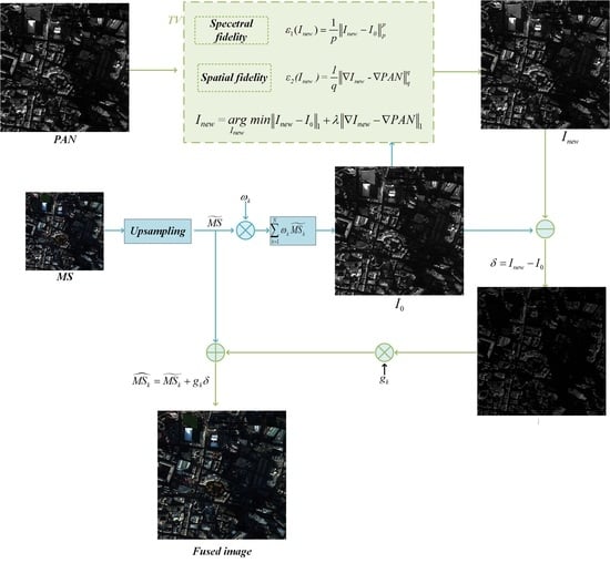
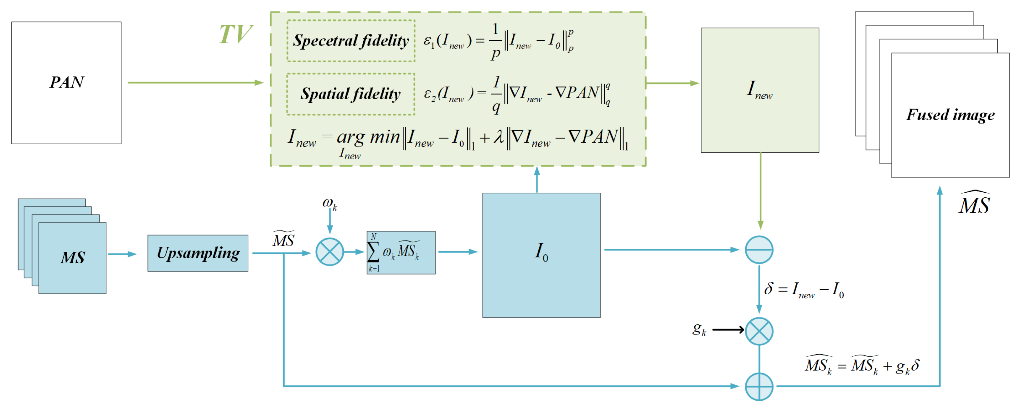
3. GIHS-TV Fusion Framework

Tu [6] simplified the component substitution framework into the details injection scheme (GIHS) by mathematical derivation. In this paper, the module for constructing new spatial components using optimization methods was integrated into the GIHS scheme, which is called the GIHS-TV framework. The general steps of the GIHS-TV framework in the component substitution method are as follows: up-sampling low-resolution multispectral images (LRMS) to PAN image size to obtain $\widehat{MS}$, calculating the spatial component (mean intensity, $I_0$) with the weights (${\omega }_k$) for LRMS bands and constructing the objective function $F(I_{\mathrm{new}},I_0,PAN)$ based on custom constraints. Then, the iterative method is selected to solve $I_{\mathrm{new}}$ by minimizing the function; according to the selected method of constructing the spatial component, the detail gain coefficients ($g_k$) are determined and the detail residuals calculated ($\delta =I_{\mathrm{new}}-I_0$). The detail injection, whose expression is as (1), is calculated to obtain the fused image.

$$\widehat{M{S}_k}=\widetilde{M{S}_k}+g_k\delta ,\forall k,$$

(1)

In addition, we proposed a new L1-TV optimized method under the GIHS-TV framework. Figure 2 clearly illustrates the construction process of the objective function and the vital role of total variation in the GIHS-TV framework.

3.1. Generalized IHS Transform

To visualize the construction process of the injection expression, we first performed the derivation of the three-channel form of the IHS method. The IHS transform extracts the spatial component ($I_0$), the hue component (H) and the saturation component (S) by performing the IHS transform on the three-channel image. The forward transform of IHS is as shown in (2).

$$\left[\begin{array}{c}\hfill I_0\hfill \\ \hfill v_1\hfill \\ \hfill v_2\hfill \end{array}\right]=\left[\begin{array}{ccc}1/3& 1/3& 1/3\\ -\sqrt{2}/6& -\sqrt{2}/6& \sqrt{2}/6\\ 1/\sqrt{2}& -1/\sqrt{2}& 0\end{array}\right]\left[\begin{array}{c}\hfill R_0\hfill \\ \hfill G_0\hfill \\ \hfill B_0\hfill \end{array}\right]$$

(2)

where $I_0$ and $I_{\mathrm{new}}$ individually represent the spatial component before and after the substitution. The inverse transformation is as shown in (3).

$$\left[\begin{array}{c}\hfill R_{\mathrm{new}}\hfill \\ \hfill G_{\mathrm{new}}\hfill \\ \hfill B_{\mathrm{new}}\hfill \end{array}\right]=\left[\begin{array}{ccc}1& -1/\sqrt{2}& 1/\sqrt{2}\\ 1& -1/\sqrt{2}& -1/\sqrt{2}\\ 1& \sqrt{2}& 0\end{array}\right]\left[\begin{array}{c}{I}_{\mathrm{new}}\\ v_1\\ v_2\end{array}\right]$$

(3)

Then, the gain coefficients and injection expression could be determined by the following.

$$\left[\begin{array}{c}{R}_{new}\\ G_{new}\\ B_{new}\end{array}\right]=\left[\begin{array}{ccc}1& -1/\sqrt{2}& 1/\sqrt{2}\\ 1& -1/\sqrt{2}& -1/\sqrt{2}\\ 1& \sqrt{2}& 0\end{array}\right]\left[\begin{array}{c}{I}_0+(I_{new}-I_0)\\ v_1\\ v_2\end{array}\right]=\left[\begin{array}{c}{R}_0+\delta \\ G_0+\delta \\ B_0+\delta \end{array}\right]$$

(4)

where ${[R_{\mathrm{new}},G_{\mathrm{new}},B_{\mathrm{new}}]}^T$ are the three channels in the fused image with the IHS method and $\delta =I_{\mathrm{new}}-I_0$. The detail injection expression for the IHS transformation is as shown in Equation (5). Thus, it is easy to determine the weights and gain coefficients in the IHS fusion method, i.e., ${\omega }_k=1/3$, $g_k=1$.

$$\widehat{M{S}_k}=\widetilde{M{S}_k}+g_k\delta =\widetilde{M{S}_k}+\left(I_{\mathrm{new}}-\frac{1}{3}\sum _{k=1}^N\widetilde{M{S}_k}\right)$$

(5)

For the GIHS method’s N-channel (N > 3) form, the GIHS transformation is as Equation (6). The spatial component’s mean intensity is synthesized as in (7).

$$\left[\begin{array}{c}{v}_1=I_0\\ v_2\\ ⋮\\ v_N\end{array}\right]=\Phi \left[\begin{array}{c}\widetilde{M{S}_1}\\ \widetilde{M{S}_2}\\ ⋮\\ \widetilde{M{S}_N}\end{array}\right]=\left[\begin{array}{cccc}{\phi }_{11}& {\phi }_{12}& \dots & {\phi }_{1N}\\ {\phi }_{21}& {\phi }_{22}& \dots & {\phi }_{2N}\\ ⋮& ⋮& & ⋮\\ {\phi }_{N1}& {\phi }_{N2}& \dots & {\phi }_{NN}\end{array}\right]\left[\begin{array}{c}\widetilde{M{S}_1}\\ \widetilde{M{S}_2}\\ ⋮\\ \widetilde{M{S}_N}\end{array}\right]$$

(6)

$$I_0=\sum _{k=1}^N{\phi }_{1k}\widetilde{M{S}_k}$$

(7)

After replacing $I_0$ with $I_{\mathrm{new}}$, the fused multispectral image could be obtained by Equation (8).

$$\begin{array}{c}\left[\begin{array}{c}\widehat{M{S}_1}\\ \widehat{M{S}_2}\\ ⋮\\ \widehat{M{S}_N}\end{array}\right]={\Phi }^{-1}\left[\begin{array}{c}{I}_{new}\\ v_2\\ ⋮\\ v_N\end{array}\right]={\Phi }^{-1}\left(\left[\begin{array}{c}{v}_1\\ v_2\\ ⋮\\ v_N\end{array}\right]+\left[\begin{array}{c}1\\ 0\\ ⋮\\ 0\end{array}\right](I_{new}-I_0)\right)\\ =\left[\begin{array}{c}\widetilde{M{S}_1}\\ \widetilde{M{S}_2}\\ ⋮\\ \widetilde{M{S}_N}\end{array}\right]+{\Phi }^{-1}\left[\begin{array}{c}1\\ 0\\ ⋮\\ 0\end{array}\right](I_{new}-I_0)\end{array}$$

(8)

where ${\Phi }^{-1}$ is the inverse of the matrix $\Phi$. From (8), it can be seen that the detail injection is only the first column of the matrix ${\Phi }^{-1}$ in action, which could be written as a new vector g. $g={[g_1,g_2,\dots ,g_N]}^T$ is called the detail gain vector. Then, Equation (8) can be written as a more concise expression for detail injection.

$$\left[\begin{array}{c}\widehat{M{S}_1}\\ \widehat{M{S}_2}\\ ⋮\\ \widehat{M{S}_N}\end{array}\right]=\left[\begin{array}{c}\widetilde{M{S}_1}\\ \widetilde{M{S}_2}\\ ⋮\\ \widetilde{M{S}_N}\end{array}\right]+g\left(I_{new}-I_0\right)=\left[\begin{array}{c}\widetilde{M{S}_1}\\ \widetilde{M{S}_2}\\ ⋮\\ \widetilde{M{S}_N}\end{array}\right]+\left[\begin{array}{c}{g}_1\\ g_2\\ ⋮\\ g_N\end{array}\right]\delta$$

(9)

Uniform detail injection form can be written as in (10)

$$\widehat{M{S}_k}=\widetilde{M{S}_k}+g_k\delta ,\forall k,$$

(10)

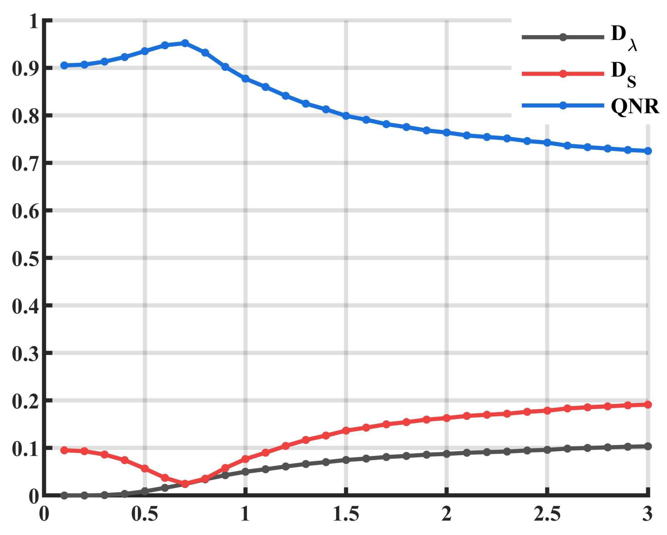
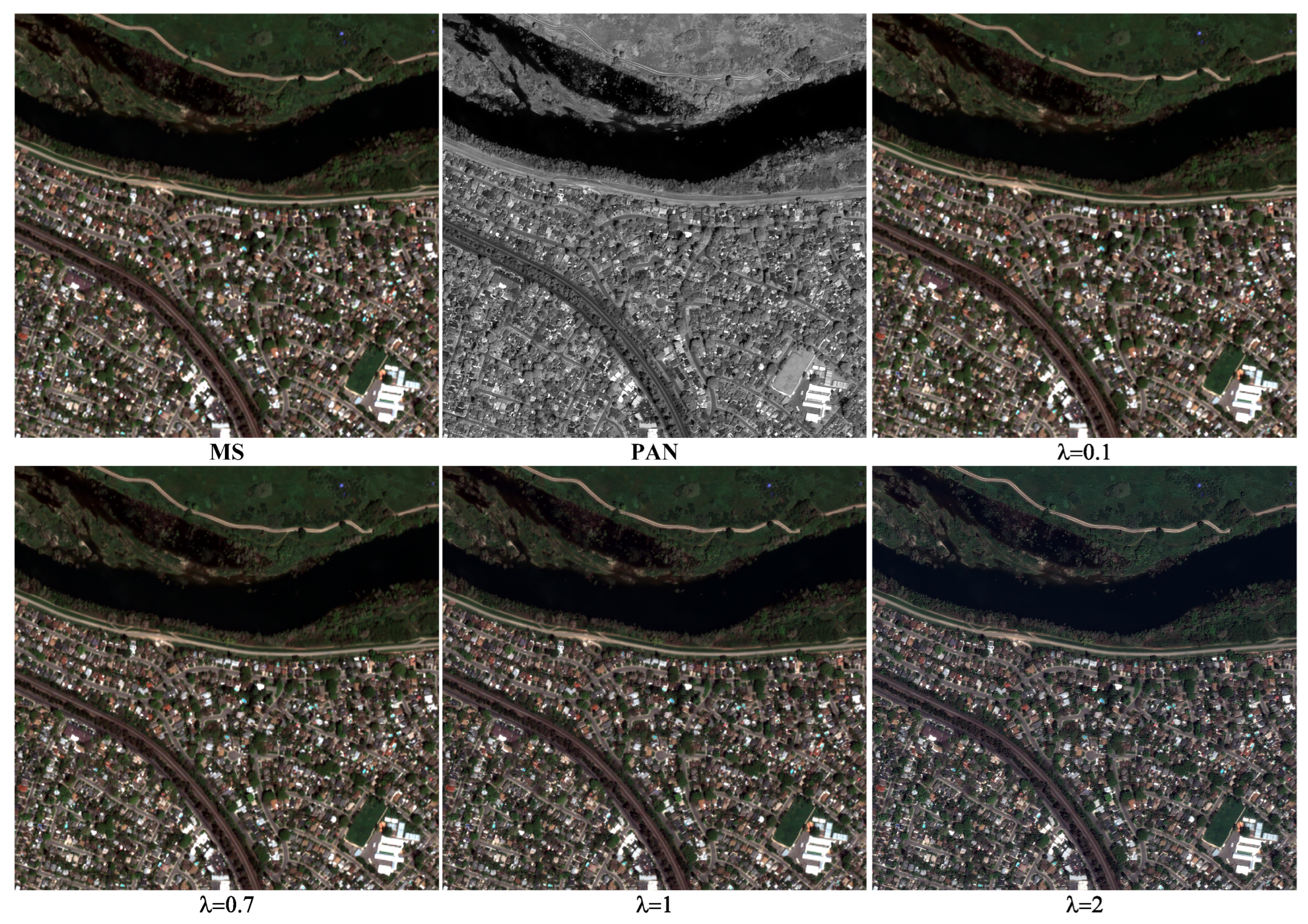
3.2. L1-TV Optimization

Due to the fact that the new spatial component could be obtained by the original spatial component and the PAN image, $I_{\mathrm{new}}$ could be regarded as the function of $I_0$ and PAN. As for the problem of spectral distortion, intensity distribution could be the most critical constraint. Combining the need to enhance the spatial detail of multispectral images, we establish the functional of the objective function for pansharpening. Specifically, the new framework (GIHS-TV) proposed in this paper considers the construction task of the new spatial component as an optimization problem.

First, the intensity distribution of the new spatial component $I_{\mathrm{new}}$ should be as consistent as possible with the spatial component $I_0$, i.e., the difference between the two should be as small as possible. To solve the problem of spectral distortion, we formulated constraints (11) as the fidelity term, which should be small enough.

$${\epsilon }_1\left(I_{\mathrm{new}}\right)=\frac{1}{p}{∥I_{\mathrm{new}}-I_0∥}_p^p$$

(11)

On the other hand, the PAN image contains more edge information. Due to the significant difference in intensity distribution between the spatial component and PAN image, it is more reasonable to use the gradient rather than the intensity to express the edge information. Therefore, the gradient of $I_{\mathrm{new}}$ should be consistent with the PAN image, and it could be regarded as the regularization item, as in Equation (12).

$${\epsilon }_2\left(I_{\mathrm{new}}\right)=\frac{1}{q}{∥\nabla I_{\mathrm{new}}-\nabla PAN∥}_q^q$$

(12)

The fusion task is then depicted as minimizing the objective function (13) to obtain spatial and spectral fidelity simultaneously.

$$\epsilon \left(I_{\mathrm{new}}\right)=\frac{1}{p}{∥I_{\mathrm{new}}-I_0∥}_p^p+\frac{\lambda }{q}{∥\nabla I_{\mathrm{new}}-\nabla PAN∥}_q^q$$

(13)

Let $p=1$, $q=1$. The rationale for the choice of the norm is as follows. Firstly, preserving the intensity distribution as much as possible is desirable, i.e., most of the fidelity term, $I_{\mathrm{new}}-I$, should be zero. From this objective, a small part of $I_{\mathrm{new}}-I$ should be large to transfer the gradient information from the PAN image to the new spatial component. The fidelity term should be subject to the Laplacian or impulsive distribution, so the L1 norm is chosen as the constraint. Secondly, the sparsity of gradients is encouraged since natural images are usually piece-wise smooth and their gradients tend to be sparse. The regularization adopted the L1 norm because relevant mathematical theory guarantees that the L1 norm can obtain the sparse solution. This objective function expects most of the difference between the $I_{\mathrm{new}}$ and $I_0$ to be zero, where the non-zero item indicates the gradient information added from the PAN image, which could ensure the sparsity of the fidelity and the consistency of intensity distribution. On the other hand, the L1 norm of the gradient, i.e., the total variation, can also encourage the sparsity of the gradient. As for the solution of the objective function, it can be turned into the L1-TV minimization problem of the variable $Diff$ with a simple variable substitution as (14) [55], and then $Diff$ can be solved by IRN [56], ADMM [57] or FISTA [58], etc. The Iteratively Reweighted Norm (IRN, [56]) method was chosen in this paper, whose stream is shown in Algorithm 1.

$$Diff=I_{new}-PAN$$

(14)

Algorithm 1 The solution flow of $Diff$ in the GIHS-TV algorithm.

Input linear operator $\mathit{A}$, image $\mathit{b}$     $\mathit{A}=\mathit{E}$ ($\mathit{E}$ is the identity matrix), $\mathit{p}=\mathit{q}=\mathbf{1}$, $\mathit{b}={\mathit{I}}_{\mathbf{0}}-\mathit{PAN}$     ${\mathit{Diff}}^{\left(\mathbf{0}\right)}={({\mathit{A}}^{\mathit{T}}\mathit{A}+\mathsf{\lambda }{\mathit{D}}^{\mathit{T}}\mathit{D})}^{-\mathbf{1}}{\mathit{A}}^{\mathit{T}}\mathit{b}$ ($\mathit{D}$ is the gradient matrix)     for   $k=0,1,\dots$do     ${\mathit{W}}_{\mathit{F}}^{\left(\mathit{k}\right)}=\mathit{diag}\left({\mathsf{\tau }}_{\mathit{F},{\mathsf{\epsilon }}_{\mathit{F}}}({\mathit{Diff}}^{\left(\mathit{k}\right)}-\mathit{b})\right)$     ${\mathit{W}}_{\mathit{R}}^{\left(\mathit{k}\right)}=\mathit{diag}({\mathsf{\tau }}_{\mathit{R},{\mathsf{\epsilon }}_{\mathit{R}}}{\left({\mathit{D}}_{\mathit{X}}{\mathit{Diff}}^{\left(\mathit{k}\right)}\right)}^{\mathbf{2}}+{\left({\mathit{D}}_{\mathit{Y}}{\mathit{Diff}}^{\left(\mathit{k}\right)}\right)}^{\mathbf{2}})$     ${\mathit{Diff}}^{(\mathit{k}+\mathbf{1})}={({\mathit{A}}^{\mathit{T}}{\mathit{W}}_{\mathit{F}}^{\left(\mathit{k}\right)}\mathit{A}+\mathsf{\lambda }{\mathit{D}}^{\mathit{T}}{\mathit{W}}_{\mathit{R}}^{\left(\mathit{k}\right)}\mathit{D})}^{-\mathbf{1}}{\mathit{A}}^{\mathit{T}}{\mathit{W}}_{\mathit{F}}^{\left(\mathit{k}\right)}\mathit{b}$    end for Output$Diff$

The new spatial component could be obtained from Equation (15). After the inverse transformation is conducted with $I_{new}$, the multispectral image with high spatial resolution is obtained.

$$I_{\mathrm{new}}=Diff+PAN$$

(15)

As for the new spatial component $I_{new}$, the simplest synthesized approach was adopted in this paper, i.e., the weight ${\omega }_k=1$, $\forall k$. In addition, the detail gain coefficient $g_k$ satisfies (16).

$$g_k={\left(\sum _{k=1}^N{\omega }_k\right)}^{-1},\forall k$$

(16)

Thus, $g_k=1$, $\forall k$. The detail residuals $\delta$ can be obtained.

$$\delta =I_{\mathrm{new}}-I_0=Diff+PAN-I_0$$

(17)

The fast implementation expression in the method with L1-TV constraints for constructing the new spatial component can be determined as in (18).

$$\widehat{M{S}_k}=\widetilde{M{S}_k}+Diff+PAN-I_0,\forall k$$

(18)

It is worth mentioning that the three-channel and the multi-channel form of the GIHS-TV share the same form of injection expression. The difference between them is only in synthesizing the mean intensity (spatial component), which brings great convenience to the two types of fusion.

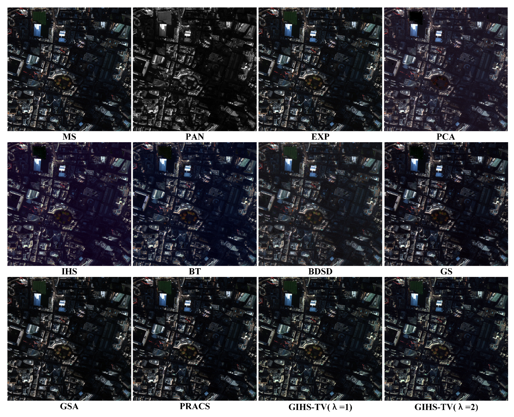
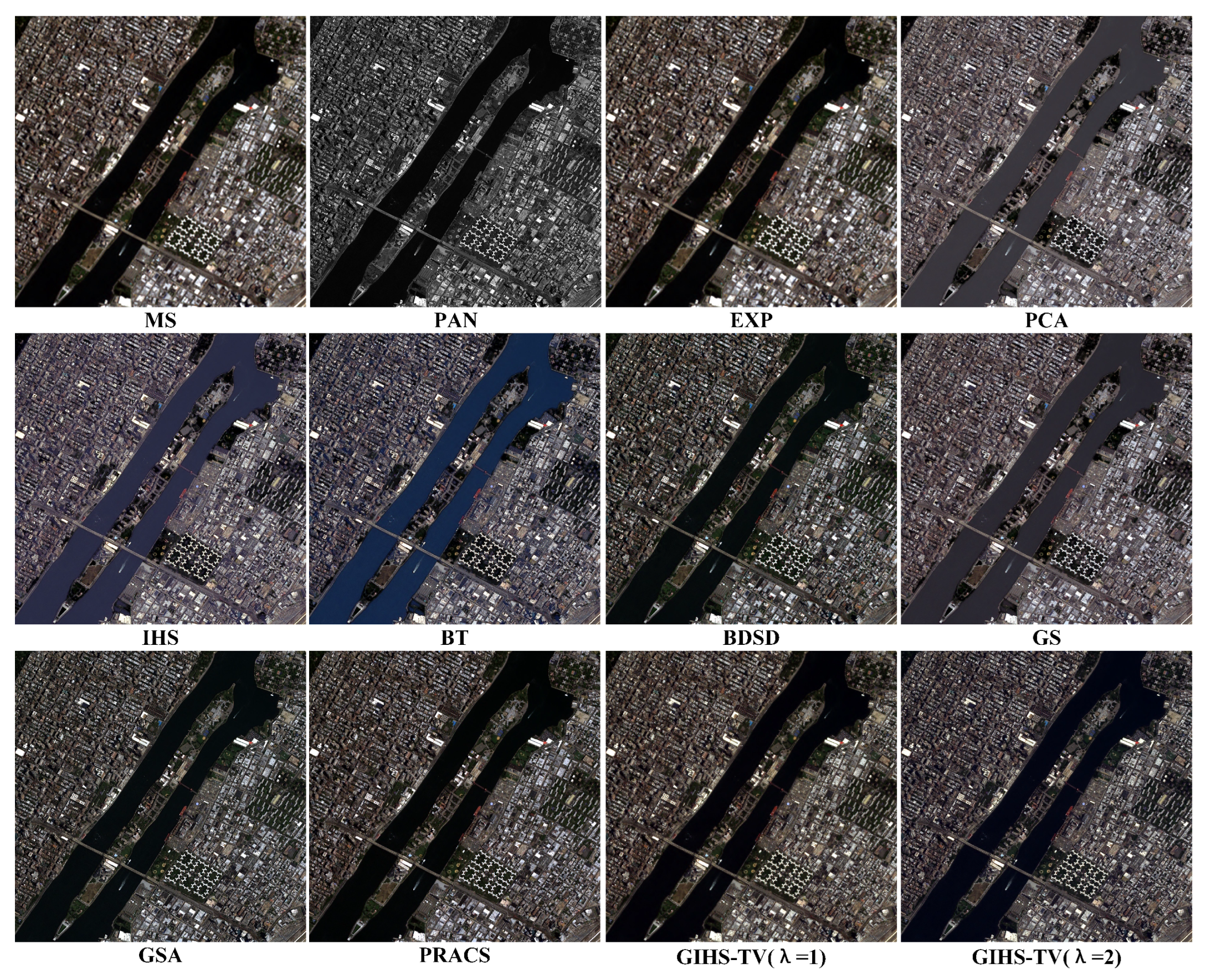
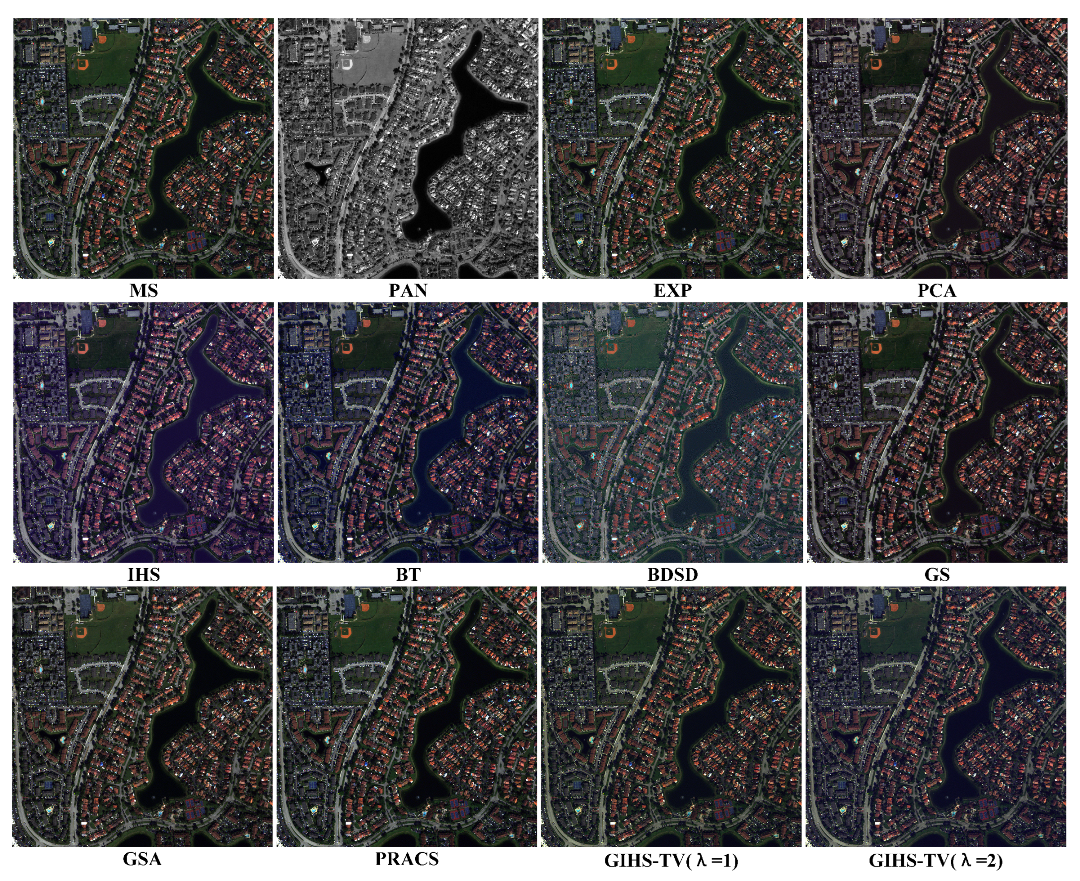
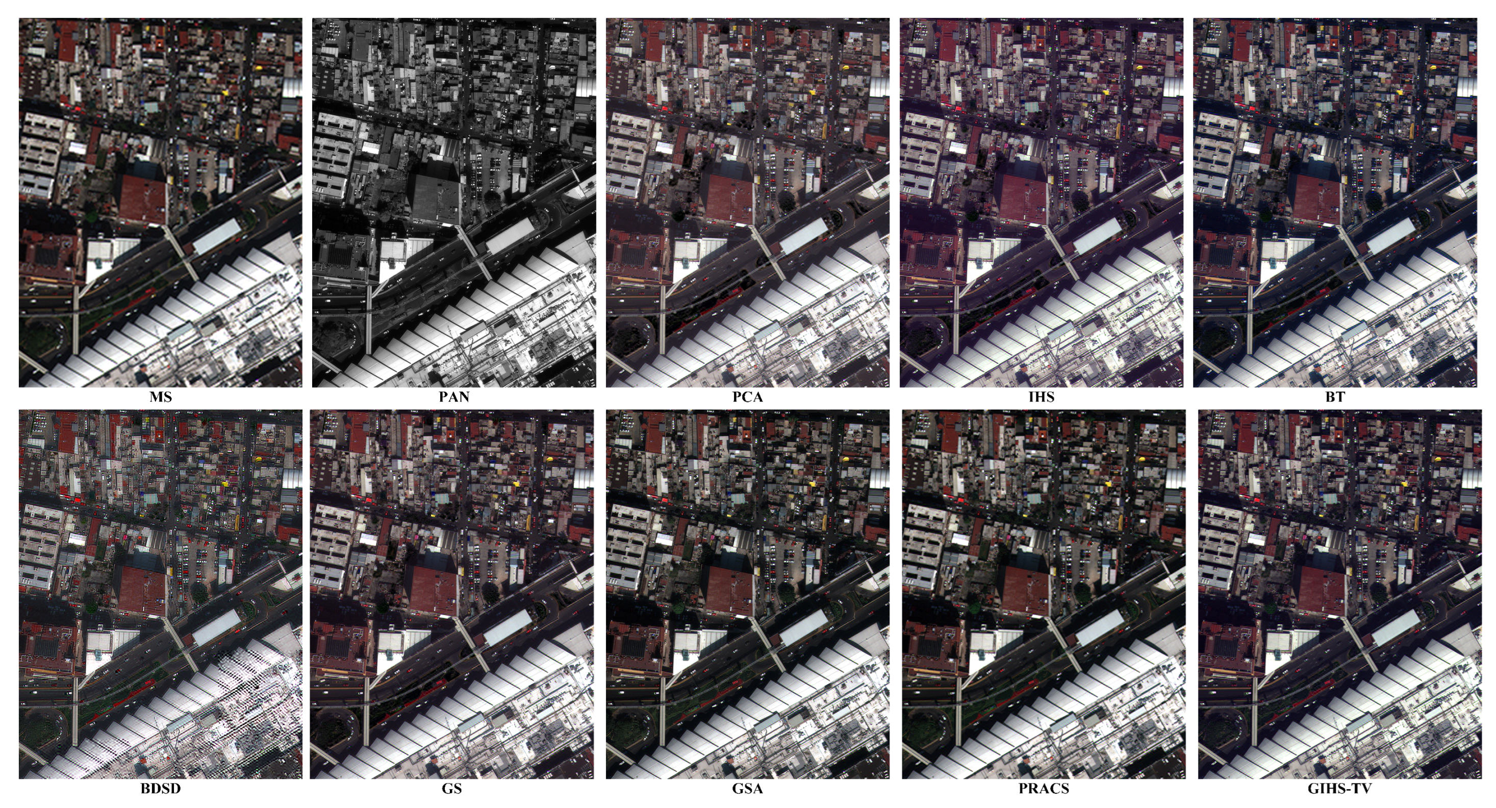
4. Experiments

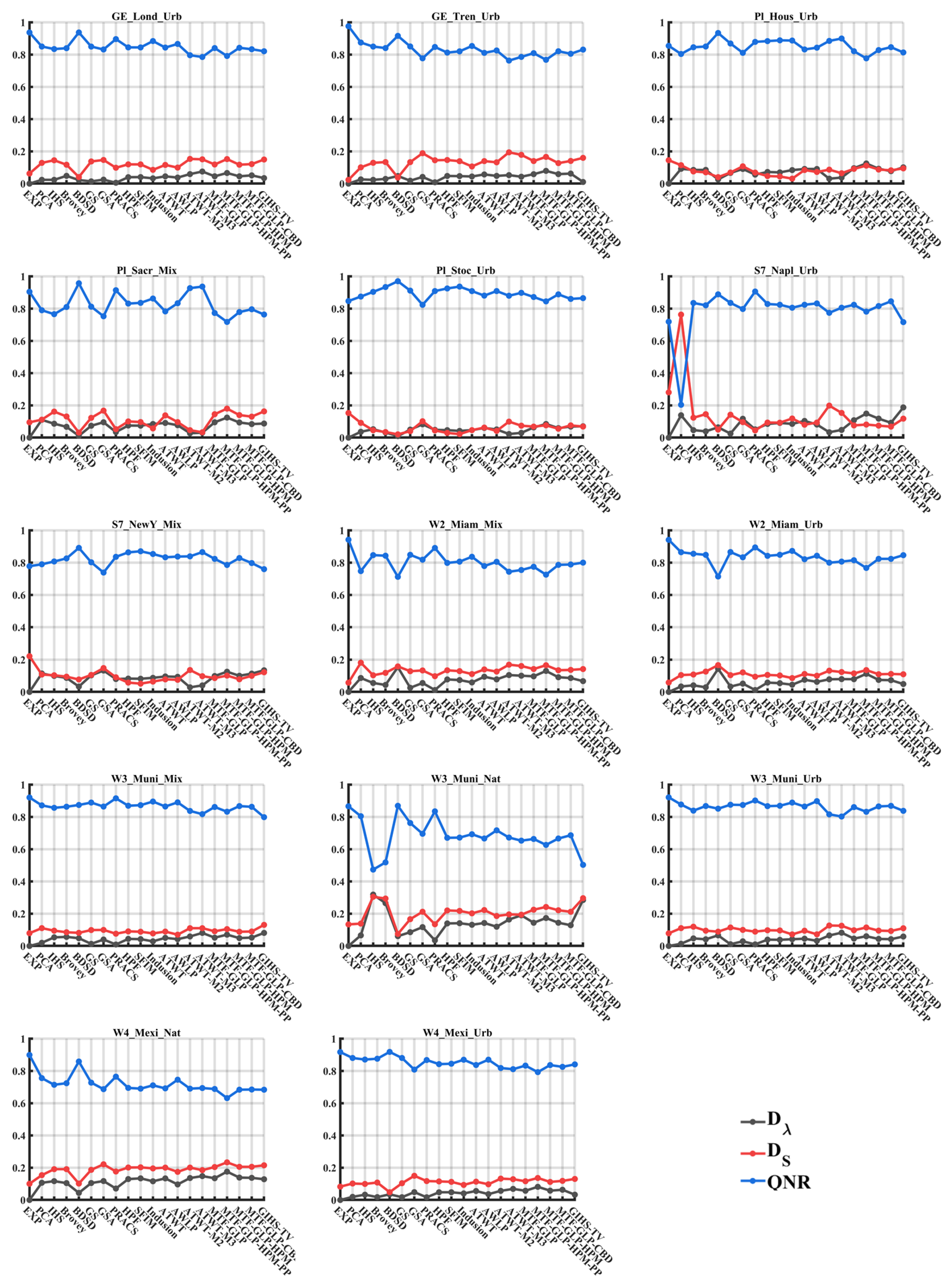
4.1. Datasets and Evaluation Metrics

In this paper, “PAirMax” [14], a publicly available fusion dataset produced by Vivone et al., was selected to explore the performance of GIHS-TV. The dataset consists of 14 pairs of images, including MS image (4-band, 8-band) and PAN image from GeoEye-1 (GE), WorldView-2 (W2), WorldView-3 (W3), WorldView-4 (W4), SPOT-7 (S7) and Pleiades (Pl), where the resolution of PAN is four times that of MS images, and the dataset has been registered. The dataset provides three types of scenarios from different countries: urban (Urb), natural (Nat) and mixed urban–natural (Mix). It shows many kinds of urban environments: typical, dense, with long shadows, water or vegetation. The data names consist of the satellite, location and scene type.

It is necessary to compare visual effects and evaluation metrics to evaluate the performance of our method. Typical CS approaches (IHS, PCA, BT, GS, GSA, BDSD, PRACS) and MRA approaches (HPF, SFIM, Indusion, ATWT, AWLP, ATWT-M2, ATWT-M3, MTF-GLP, MTF-GLP-HPM-PP, MTF-GLP-CBD) were chosen to conduct the comparison with GIHS-TV in the full resolution fusion. The retention of spectral and spatial details is quantitatively evaluated by the selected evaluation metrics, such as spectral angle (SAM) [59], spatial correlation coefficient (SCC) [60], $D_{\lambda }$ [61], $D_S$ [61] and QNR [61]. The details of these metrics are as follows.

(1) SAM: SAM reflects the spectral fidelity between the fused image and the reference MS images by calculating the spectral angle between the corresponding pixels of the two images. Denote $F\left\{i\right\}$ and $R\left\{i\right\}$ as the grayscale values at position i in the fused and MS images, respectively. The calculation is as in Equation (19).

$$SAM\left(F\left\{i\right\},R\left\{i\right\}\right)=arccos\left(\frac{〈F\left\{i\right\},R\left\{i\right\}〉}{∥F\left\{i\right\}∥∥R\left\{i\right\}∥}\right)$$

(19)

The average of the spectral angle of all pixels is regarded as the SAM of the two images. The smaller the SAM value, the higher the spectral fidelity.

(2) SCC: The high-frequency information is extracted from the PAN and fused images by high-pass filters; then, the correlation between the two is calculated through correlation coefficients. Its definition is as Equation (20).

$$SCC=\frac{{\displaystyle \sum _{i=1}^M}{\displaystyle \sum _{j=1}^N}(H{F}_k^{\prime }(i,j)-\overline{H{F}_k^{\prime }})(HP(i,j)-\overline{HP})}{\sqrt{{\displaystyle \sum _{i=1}^M}{\displaystyle \sum _{j=1}^N}{(H{F}_k^{\prime }(i,j)-\overline{H{F}_k^{\prime }})}^2}\sqrt{{\displaystyle \sum _{i=1}^M}{\displaystyle \sum _{j=1}^N}{(HP(i,j)-\overline{HP})}^2}}$$

(20)

where $H{F}_k^{\prime }$ stands for the high-frequency information of the kth band in the fused images, and $HP$ is the high-frequency information of the PAN image. The larger the SCC, the better the spatial correlation between the fused and the PAN images.

(3) $D_{\lambda }$: $D_{\lambda }$ characterizes the spectral loss between the fused and the MS images and is defined by the following equation.

$$D_{\lambda }=\sqrt[p]{\frac{1}{B(B-1)}\sum _{i=1}^B\sum _{\genfrac{}{}{0pt}{}{j=1}{j\ne i}}^B{\left|Q(F_i,F_j)-Q(M{S}_i,M{S}_j)\right|}^p}$$

(21)

where p amplifies the spectral differences and is usually set to 1. The smaller it is, the smaller the spectral distortion is. Q is the universal image quality index (UIQI). UIQI calculates the correlation, brightness and contrast similarity between the fused and the reference images to characterize the comprehensive performance of fusion. It is usually abbreviated as the Q index, and the definition formula is as follows.

$$Q(F,R)=\frac{{\sigma }_{FR}}{{\sigma }_F{\sigma }_R}\frac{2{\mu }_F{\mu }_R}{{\mu }_F^2+{\mu }_R^2}\frac{2{\sigma }_F{\sigma }_R}{{\sigma }_F^2+{\sigma }_R^2}$$

(22)

where ${\sigma }_F$ and ${\sigma }_R$ are the standard deviations of the fused and the reference images, respectively, ${\sigma }_{FR}$ is the covariance of the two, and ${\mu }_F$ and ${\mu }_R$ denote the mean values of the two, respectively. The three fractions represent the correlation, mean brightness and contrast similarity. The higher Q value means that the fused images are more similar to the reference images.

(4) $D_S$: $D_S$ is used to calculate the loss of spatial detail between the fused and the PAN images. It is defined by the following.

$$D_S=\sqrt[q]{\frac{1}{B}\sum _{i=1}^B{\left|Q(F_i,PAN)-Q(M{S}_i,PA{N}_{LP})\right|}^q}$$

(23)

where $PA{N}_{LP}$ is the downsampled PAN image to the same resolution as the original MS images. From a practical point of view, it should be ensured that the $PA{N}_{LP}$ should be perfectly aligned with the MS image; otherwise, this metric loses its meaning. q serves to amplify the difference in spatial detail distortion. The smaller the $D_S$, the smaller the spatial detail distortion is.

(5) $QNR$: $QNR$ is the most mainstream non-reference index for evaluating the performance of pansharpening methods, which integrates spectral and spatial distortion characterization, as defined below.

$$QNR={(1-D_{\lambda })}^{\alpha }{(1-D_S)}^{\beta }$$

(24)

where $\alpha$ and $\beta$ are parameters used to balance the spectral distortion and spatial distortion, and the larger the QNR, the better the fusion performance, with a maximum value of 1.

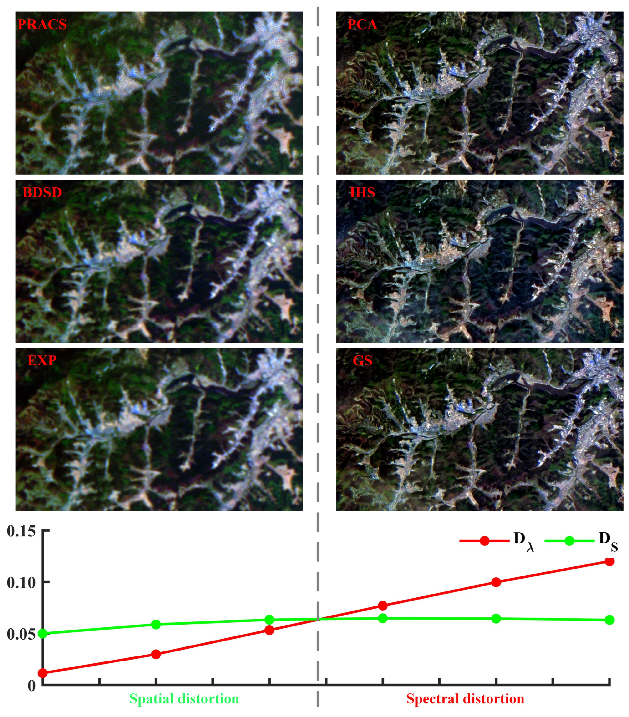
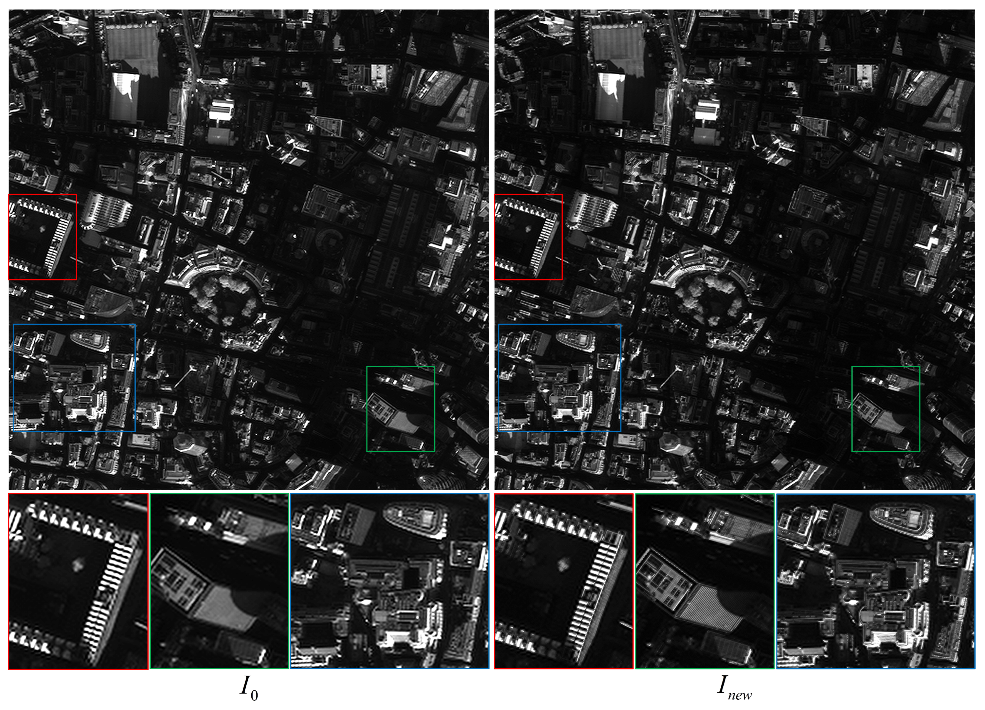
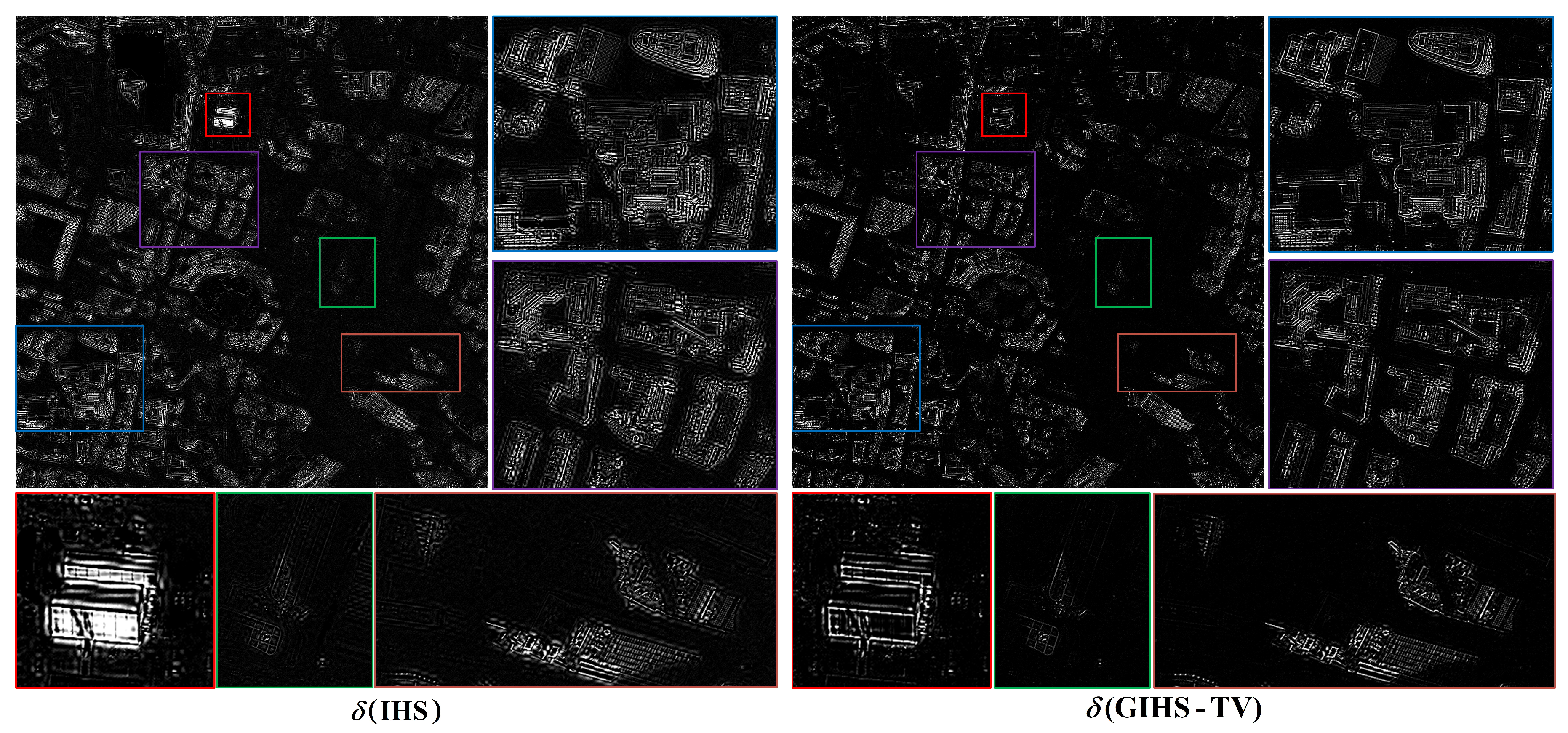
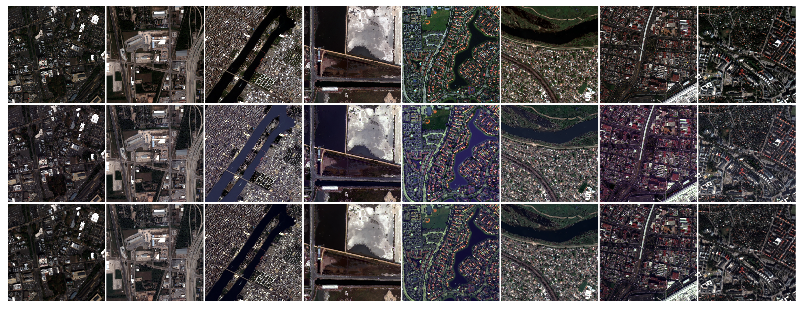
4.2. Initial Results

In the GIHS-TV framework, the residuals between the new and original spatial components ($I_0$ and $I_{\mathrm{new}}$) stand for the detail injections added to the fused images. The consistency and difference were analyzed in the global and local performance. In addition, the residual by the IHS method was provided for comparison with the one of the GIHS-TV methods.

The experiments in the scene “GE_Lond_Urb” show the spatial component images before and after the fusion. Figure 3 shows that the two images maintain a good consistency in global hue, which indicates the spectral fidelity of the GIHS-TV method. In the boxes, the texture and contour of the buildings in the $I_{\mathrm{new}}$ is richer than that in the $I_0$. Further, the residuals ($\delta$) between $I_0$ and $I_{\mathrm{new}}$ were evaluated in terms of the grayscale and edge. A histogram stretching was performed on the residuals. Another implication of the residuals is the detail injection in our framework, which accounts for the selection of the IHS method for the auxiliary analysis where the two methods share the same $I_0$ and our method produces the new spatial component by L1-TV.

In Figure 4, clear edges were shown in the residuals from the GIHS-TV method, achieving the goal of adding edge information from the PAN image to $I_{\mathrm{new}}$ without altering the grayscale distribution as much as possible. Many artifacts near the edges were generated in the residuals from the IHS method. Especially, the interior of the building was almost filled with white in the red box; a dramatic brightness changes occurred in the new spatial component, and the final fused images showed spectral distortion. Several other local details are present in Figure 4—our method also has good, cleaner edge details.

The proportion of edge information added from the PAN image was changed through hyperparameter $\lambda$ in the model. The fused effects of $\lambda$ values were analyzed in terms of both visual effects and evaluation metrics in the “Pl_Sacr_Mix” scene. Figure 5 shows that the results are consistent with the intuition that as the hyperparameter increases, the geometric information becomes richer while the spectral distortion increases. At the same time, there is a tipping point ($\lambda$ = 0.7) and a bottleneck point ($\lambda$ = 2.8). $D_S$, and QNR achieves the best value at $\lambda$ = 0.7, but the visual results of the fusion in Figure 6 show a good balance between spectral fidelity and spatial fidelity when $\lambda$ is equal to 1.

4.3. Fusion Results

Images by EXP [3] stand for the MS image interpolation using a polynomial kernel with 23 coefficients. The hyperparameters $\lambda$ in the GIHS-TV method were set to 1 and 2, and the parameters of the other methods were kept consistent with the corresponding articles. Experiments on the “PAirMax” dataset show that most fusion methods enhance spatial details compared with the original MS images. Objects that cannot be identified in any single original image can be easily identified and inferred in fused images. However, CS approaches exhibit various degrees of color distortion. Fused images of typical scenes were shown and analyzed.

In the “GE_Lond_Urb” (Figure 7), the fused images all perform well in the enhancement of spatial details. The details within the shadows are enhanced well, such as the cars and the color, contours and texture of the trees and the low buildings. The textures of the tall buildings outside the shadows also become apparent, and even their structures or materials can be inferred. However, PCA, IHS and GS all exhibit a global blue hue that is different from the original MS image. This shows the color distortion that occurred in the CS approaches. In contrast, GIHS-TV performs better in terms of global hue and the spectral construction of local objects.

In the “S7_NewY_Mix” (Figure 8), the most conspicuous feature is the river and the global hue. The spectral construction of the river by the PCA, IHS, BT and GS shows apparent errors. Regarding the spectral construction of vegetation and buildings, only four improved CS methods, GSA, BDSD, PRACS and GIHS-TV, have superior performances.

In the “W2_Miam_Mix” (Figure 9), we mainly reference the color of the grass and trees and the global hue. The PCA, IHS, BT and BDSD methods show poor global hue, and BDSD performs poorly in spatial expression. It is worth pointing out that the GIHS-TV method contains richer spatial details when the hyperparameter is greater than or equal to 2 but also exhibits color distortion, which also occurs in Figure 8. If the fused images were to be used for the visual tasks, a large $\lambda$ value would work better, $\lambda =2$, which is recommended as an experience value based on our experimental results.

In the local of “Pl_Hous_Urb” (Figure 10), the fused images of all methods are rich in spatial details, especially the target contours and textures of cargo bins, trucks plants. In addition, road lines are effectively enhanced. GIHS-TV achieved a visual effect comparable to other methods.

The local fused results of “W4_Mexi_Urb” are as shown in Figure 11, where the spatial details in the fused images are rich. It can be seen that, compared with other methods, the PRACS method is slightly weaker in rendering spatial details, such as the poor clarity of buildings’ contours. The BDSD method tends to introduce spatial artifacts. These two improved CS-based methods are centered on spectral fidelity and do not use the PAN directly when constructing the spatial component but use its downsampled PAN or its partial image, and their spatial detail injection is not as good as other methods, which explains the lack of effective improvement in their spatial fidelity. GIHS-TV fused images perform well in both spectral fidelity and spatial fidelity, and it can effectively identify many small targets, such as buildings, cars, containers and objects on building roofs.

The experimental performance with high spatial and spectral fidelity fully illustrates the advantages of the GIHS-TV framework for constructing spatial components with optimized ideas. GIHS-TV achieved a superior performance.

Representative methods of CS and MRA were selected for the comparison and evaluation of fusion methods in the full-resolution scheme provided by Vivone [5,11]. As shown in Figure 12, it can be seen that the evaluation metrics of the GIHS-TV method fusion perform well, with lower $D_{\lambda }$ and higher QNR in most scenes. The lower $D_{\lambda }$ indicates good performance in spectral fidelity, and a higher QNR stands for an excellent comprehensive fidelity.

Among the many methods, only the BDSD method can outperform the GIHS-TV metrics in most scenes, but based on the visual analysis above, it is clear that BDSD does not perform as well as GIHS-TV and other methods.

The above visual effects show that the GIHS-TV method effectively improves the spectral distortion in the component substitution class. The analysis of the evaluation metrics shows better performances than these methods. A comparison with MRA-based methods was conducted and shown.

Table 1. The mean evaluation metrics of fusion on the “PAirMax” dataset. Numbers in the bold stands for the best values.

Method	${\mathit{D}}_{\mathit{\lambda }}$	${\mathit{D}}_{\mathit{S}}$	QNR	SAM	SCC
HPF	0.0651	0.1031	0.8389	1.5775	0.8600
SFIM	0.0644	0.0998	0.8427	1.2277	0.8559
Indusion	0.0613	0.0882	0.8562	2.7859	0.8040
ATWT	0.0769	0.1115	0.8206	1.8998	0.8738
AWLP	0.0637	0.0964	0.8463	2.0627	0.8302
ATWT-M2	0.0581	0.1375	0.8132	2.0203	0.8408
ATWT-M3	0.0666	0.1221	0.8203	1.9297	0.8606
MTF-GLP	0.0794	0.1149	0.8152	2.0113	0.8789
MTF-GLP-HPM-PP	0.1065	0.1354	0.7730	2.4969	0.8948
MTF-GLP-HPM	0.0788	0.1097	0.8206	1.4539	0.8707
MTF-GLP-CBD	0.0773	0.1135	0.8184	2.1497	0.8742
GIHS-TV ($\lambda =1$)	0.0550	0.0876	0.8624	0.6090	0.8760

offers the mean value of six metrics undertaken in the 13 scenes except for the “W3_Muni_Nat”. The GIHS-TV performs best in all full resolution metrics i.e., $D_{\lambda }$, $D_{\S }$, QNR. As for the performance at reduced resolution, our method behaves well in both SAM and SCC. In Figure 13, GIHS-TV performs with high spectral fidelity and more spatial details compared with the IHS method and LRMS images, whose performance is consistent with those at full resolution.

Compared with ATWT-M2 and ATWT-M3 methods, GIHS-TV needs a slightly longer computation time due to optimization iterations. It is more meaningful to make comparisons between the same class of methods. Thus, the P+XS methods are selected to compare the running time in the “GE_Tren_Urb”, “W3_Muni_Urb”, “W3_Muni_Mix” and “W4_Mexi_Nat” scenes. As shown in

Table 2. The calculation time of P+XS and GIHS-TV (seconds).

Methods	GE_Tren_Urb	W3_Muni_Urb	W3_Muni_Mix	W4_Mexi_Nat
P+XS	197.7686	397.8795	420.6308	207.6450
GIHS-TV	27.6508	23.0162	26.5074	24.2559

, the optimization times of the GIHS-TV method are much lower than the P+XS method—approximately one order of magnitude. This is attributed to the sparsity and conciseness of the proposed model.

The analysis involving visual effects and metrics shows that the GIHS-TV method is excellent in terms of fusion with high spectral and spatial fidelity. Compared with traditional TV-based methods, our method performs with better timeliness.

5. Conclusions

This paper adopted an optimization perspective to improve the CS-based pansharpening methods and build the GIHS-TV framework. Faced with the problem of the loss of spectral information in the fused images, we proposed a method with L1-TV that was used to constrain the spectral–spatial information in the new spatial components, effectively improving the spectral distortion. Its fast algorithm was implemented in the framework. Compared with other variational optimization-based methods, the GIHS-TV framework absorbs the advantage of high spatial fidelity from the CS-based methods. Experiments on the “PairMax” dataset show that GIHS-TV can maintain both the spectral and spatial information from the MS and PAN image well. The spectral fidelity in GIHS-TV is greatly improved compared with other CS approaches.

References

- Edwards, K.; Davis, P.A. The use of intensity-hue-saturation transformation for producing color shaded-relief images. Photogramm. Eng. Remote Sens. 1994, 60, 1369–1374. [Google Scholar]
- Laben, C.A.; Brower, B.V. Process for Enhancing the Spatial Resolution of Multispectral Imagery Using Pan-Sharpening. U.S. Patent 6,011,875, 4 January 2000. [Google Scholar]
- Aiazzi, B.; Alparone, L.; Baronti, S.; Garzelli, A. Context-driven fusion of high spatial and spectral resolution images based on oversampled multiresolution analysis. IEEE Trans. Geosci. Remote Sens. 2002, 40, 2300–2312. [Google Scholar] [CrossRef]
- Garzelli, A.; Nencini, F.; Capobianco, L. Optimal MMSE pan sharpening of very high resolution multispectral images. IEEE Trans. Geosci. Remote Sens. 2007, 46, 228–236. [Google Scholar] [CrossRef]
- Vivone, G.; Dalla Mura, M.; Garzelli, A.; Restaino, R.; Scarpa, G.; Ulfarsson, M.O.; Alparone, L.; Chanussot, J. A new benchmark based on recent advances in multispectral pansharpening: Revisiting pansharpening with classical and emerging pansharpening methods. IEEE Geosci. Remote Sens. Mag. 2020, 9, 53–81. [Google Scholar] [CrossRef]
- Tu, T.M.; Su, S.C.; Shyu, H.C.; Huang, P.S. A new look at IHS-like image fusion methods. Inf. Fusion 2001, 2, 177–186. [Google Scholar] [CrossRef]
- Javan, F.D.; Samadzadegan, F.; Mehravar, S.; Toosi, A.; Khatami, R.; Stein, A. A review of image fusion techniques for pan-sharpening of high-resolution satellite imagery. ISPRS J. Photogramm. Remote Sens. 2021, 171, 101–117. [Google Scholar] [CrossRef]
- Vivone, G.; Restaino, R.; Dalla Mura, M.; Licciardi, G.; Chanussot, J. Contrast and error-based fusion schemes for multispectral image pansharpening. IEEE Geosci. Remote Sens. Lett. 2013, 11, 930–934. [Google Scholar] [CrossRef] [Green Version]
- Ranchin, T.; Wald, L. Fusion of high spatial and spectral resolution images: The ARSIS concept and its implementation. Photogramm. Eng. Remote Sens. 2000, 66, 49–61. [Google Scholar]
- Aiazzi, B.; Alparone, L.; Baronti, S.; Garzelli, A.; Selva, M. MTF-tailored multiscale fusion of high-resolution MS and Pan imagery. Photogramm. Eng. Remote Sens. 2006, 72, 591–596. [Google Scholar] [CrossRef]
- Vivone, G.; Alparone, L.; Chanussot, J.; Dalla Mura, M.; Garzelli, A.; Licciardi, G.A.; Restaino, R.; Wald, L. A critical comparison among pansharpening algorithms. IEEE Trans. Geosci. Remote Sens. 2014, 53, 2565–2586. [Google Scholar] [CrossRef]
- Otazu, X.; González-Audícana, M.; Fors, O.; Núñez, J. Introduction of sensor spectral response into image fusion methods. Application to wavelet-based methods. IEEE Trans. Geosci. Remote Sens. 2005, 43, 2376–2385. [Google Scholar] [CrossRef] [Green Version]
- Liu, P.; Xiao, L.; Tang, S.; Sun, L. Fractional order variational pan-sharpening. In Proceedings of the 2016 IEEE International Geoscience and Remote Sensing Symposium (IGARSS), Beijing, China, 10–15 July 2016; pp. 2602–2605. [Google Scholar]
- Vivone, G.; Dalla Mura, M.; Garzelli, A.; Pacifici, F. A benchmarking protocol for pansharpening: Dataset, preprocessing, and quality assessment. IEEE J. Sel. Top. Appl. Earth Obs. Remote Sens. 2021, 14, 6102–6118. [Google Scholar] [CrossRef]
- Li, S.; Yang, B. A new pan-sharpening method using a compressed sensing technique. IEEE Trans. Geosci. Remote Sens. 2010, 49, 738–746. [Google Scholar] [CrossRef]
- Li, S.; Yin, H.; Fang, L. Remote sensing image fusion via sparse representations over learned dictionaries. IEEE Trans. Geosci. Remote Sens. 2013, 51, 4779–4789. [Google Scholar] [CrossRef]
- Zhong, J.; Yang, B.; Huang, G.; Zhong, F.; Chen, Z. Remote sensing image fusion with convolutional neural network. Sens. Imaging 2016, 17, 10. [Google Scholar] [CrossRef]
- Li, Z.; Cheng, C. A CNN-based pan-sharpening method for integrating panchromatic and multispectral images using Landsat 8. Remote Sens. 2019, 11, 2606. [Google Scholar] [CrossRef] [Green Version]
- Zeng, Z.; Wang, D.; Tan, W.; Yu, G.; You, J.; Lv, B.; Wu, Z. RCSANet: A Full Convolutional Network for Extracting Inland Aquaculture Ponds from High-Spatial-Resolution Images. Remote Sens. 2020, 13, 92. [Google Scholar] [CrossRef]
- Wang, W.; Zhou, Z.; Liu, H.; Xie, G. MSDRN: Pansharpening of multispectral images via multi-scale deep residual network. Remote Sens. 2021, 13, 1200. [Google Scholar] [CrossRef]
- Liu, Q.; Han, L.; Tan, R.; Fan, H.; Li, W.; Zhu, H.; Du, B.; Liu, S. Hybrid attention based residual network for pansharpening. Remote Sens. 2021, 13, 1962. [Google Scholar] [CrossRef]
- Wu, Y.; Feng, S.; Lin, C.; Zhou, H.; Huang, M. A three stages detail injection network for remote sensing images pansharpening. Remote Sens. 2022, 14, 1077. [Google Scholar] [CrossRef]
- Yin, J.; Qu, J.; Sun, L.; Huang, W.; Chen, Q. A Local and Nonlocal Feature Interaction Network for Pansharpening. Remote Sens. 2022, 14, 3743. [Google Scholar] [CrossRef]
- Nie, Z.; Chen, L.; Jeon, S.; Yang, X. Spectral-Spatial Interaction Network for Multispectral Image and Panchromatic Image Fusion. Remote Sens. 2022, 14, 4100. [Google Scholar] [CrossRef]
- Jian, L.; Wu, S.; Chen, L.; Vivone, G.; Rayhana, R.; Zhang, D. Multi-Scale and Multi-Stream Fusion Network for Pansharpening. Remote Sens. 2023, 15, 1666. [Google Scholar] [CrossRef]
- Ciotola, M.; Scarpa, G. Fast Full-Resolution Target-Adaptive CNN-Based Pansharpening Framework. Remote Sens. 2023, 15, 319. [Google Scholar] [CrossRef]
- Ma, J.; Yu, W.; Chen, C.; Liang, P.; Guo, X.; Jiang, J. Pan-GAN: An unsupervised pan-sharpening method for remote sensing image fusion. Inf. Fusion 2020, 62, 110–120. [Google Scholar] [CrossRef]
- Zhang, L.; Li, W.; Huang, H.; Lei, D. A pansharpening generative adversarial network with multilevel structure enhancement and a multistream fusion architecture. Remote Sens. 2021, 13, 2423. [Google Scholar] [CrossRef]
- Gastineau, A.; Aujol, J.F.; Berthoumieu, Y.; Germain, C. Generative adversarial network for pansharpening with spectral and spatial discriminators. IEEE Trans. Geosci. Remote Sens. 2021, 60, 4401611. [Google Scholar] [CrossRef]
- Liu, Q.; Zhou, H.; Xu, Q.; Liu, X.; Wang, Y. PSGAN: A generative adversarial network for remote sensing image pan-sharpening. IEEE Trans. Geosci. Remote Sens. 2020, 59, 10227–10242. [Google Scholar] [CrossRef]
- Jozdani, S.; Chen, D.; Chen, W.; Leblanc, S.G.; Lovitt, J.; He, L.; Fraser, R.H.; Johnson, B.A. Evaluating Image Normalization via GANs for Environmental Mapping: A Case Study of Lichen Mapping Using High-Resolution Satellite Imagery. Remote Sens. 2021, 13, 5035. [Google Scholar] [CrossRef]
- Masi, G.; Cozzolino, D.; Verdoliva, L.; Scarpa, G. Pansharpening by convolutional neural networks. Remote Sens. 2016, 8, 594. [Google Scholar] [CrossRef] [Green Version]
- Choi, J.; Yu, K.; Kim, Y. A new adaptive component-substitution-based satellite image fusion by using partial replacement. IEEE Trans. Geosci. Remote Sens. 2010, 49, 295–309. [Google Scholar] [CrossRef]
- Carper, W.; Lillesand, T.; Kiefer, R. The use of intensity-hue-saturation transformations for merging SPOT panchromatic and multispectral image data. Photogramm. Eng. Remote Sens. 1990, 56, 459–467. [Google Scholar]
- Kwarteng, P.; Chavez, A. Extracting spectral contrast in Landsat Thematic Mapper image data using selective principal component analysis. Photogramm. Eng. Remote Sens. 1989, 55, 339–348. [Google Scholar]
- Gillespie, A.R.; Kahle, A.B.; Walker, R.E. Color enhancement of highly correlated images. II. Channel ratio and “chromaticity” transformation techniques. Remote Sens. Environ. 1987, 22, 343–365. [Google Scholar] [CrossRef]
- Aiazzi, B.; Baronti, S.; Selva, M. Improving component substitution pansharpening through multivariate regression of MS + Pan data. IEEE Trans. Geosci. Remote Sens. 2007, 45, 3230–3239. [Google Scholar] [CrossRef]
- Vivone, G. Robust band-dependent spatial-detail approaches for panchromatic sharpening. IEEE Trans. Geosci. Remote Sens. 2019, 57, 6421–6433. [Google Scholar] [CrossRef]
- Aiazzi, B.; Alparone, L.; Baronti, S.; Garzelli, A.; Selva, M. An MTF-based spectral distortion minimizing model for pan-sharpening of very high resolution multispectral images of urban areas. In Proceedings of the 2003 2nd GRSS/ISPRS Joint Workshop on Remote Sensing and Data Fusion over Urban Areas, Berlin, Germany, 22–23 May 2003; pp. 90–94. [Google Scholar]
- Chavez, P.; Sides, S.C.; Anderson, J.A. Comparison of three different methods to merge multiresolution and multispectral data- Landsat TM and SPOT panchromatic. Photogramm. Eng. Remote Sens. 1991, 57, 295–303. [Google Scholar]
- Khan, M.M.; Chanussot, J.; Condat, L.; Montanvert, A. Indusion: Fusion of multispectral and panchromatic images using the induction scaling technique. IEEE Geosci. Remote Sens. Lett. 2008, 5, 98–102. [Google Scholar] [CrossRef] [Green Version]
- Liu, J. Smoothing filter-based intensity modulation: A spectral preserve image fusion technique for improving spatial details. Int. J. Remote Sens. 2000, 21, 3461–3472. [Google Scholar] [CrossRef]
- Wald, L.; Ranchin, T. Liu’Smoothing filter-based intensity modulation: A spectral preserve image fusion technique for improving spatial details’. Int. J. Remote Sens. 2002, 23, 593–597. [Google Scholar] [CrossRef]
- Dong, W.; Xiao, S.; Li, Y.; Qu, J. Hyperspectral pansharpening based on intrinsic image decomposition and weighted least squares filter. Remote Sens. 2018, 10, 445. [Google Scholar] [CrossRef] [Green Version]
- Ballester, C.; Caselles, V.; Igual, L.; Verdera, J.; Rougé, B. A variational model for P+ XS image fusion. Int. J. Comput. Vis. 2006, 69, 43. [Google Scholar] [CrossRef]
- Palsson, F.; Sveinsson, J.R.; Ulfarsson, M.O. A new pansharpening algorithm based on total variation. IEEE Geosci. Remote Sens. Lett. 2013, 11, 318–322. [Google Scholar] [CrossRef]
- He, X.; Condat, L.; Bioucas-Dias, J.M.; Chanussot, J.; Xia, J. A new pansharpening method based on spatial and spectral sparsity priors. IEEE Trans. Image Process. 2014, 23, 4160–4174. [Google Scholar] [CrossRef] [PubMed]
- Tian, X.; Chen, Y.; Yang, C.; Gao, X.; Ma, J. A variational pansharpening method based on gradient sparse representation. IEEE Signal Process. Lett. 2020, 27, 1180–1184. [Google Scholar] [CrossRef]
- Fasbender, D.; Radoux, J.; Bogaert, P. Bayesian data fusion for adaptable image pansharpening. IEEE Trans. Geosci. Remote Sens. 2008, 46, 1847–1857. [Google Scholar] [CrossRef]
- Möller, M.; Wittman, T.; Bertozzi, A.L.; Burger, M. A variational approach for sharpening high dimensional images. SIAM J. Imaging Sci. 2012, 5, 150–178. [Google Scholar] [CrossRef] [Green Version]
- Zhang, G.; Fang, F.; Zhou, A.; Li, F. Pan-sharpening of multi-spectral images using a new variational model. Int. J. Remote Sens. 2015, 36, 1484–1508. [Google Scholar] [CrossRef]
- Duran, J.; Buades, A.; Coll, B.; Sbert, C. A nonlocal variational model for pansharpening image fusion. SIAM J. Imaging Sci. 2014, 7, 761–796. [Google Scholar] [CrossRef]
- Yang, J.; Fu, X.; Hu, Y.; Huang, Y.; Ding, X.; Paisley, J. PanNet: A deep network architecture for pan-sharpening. In Proceedings of the IEEE International Conference on Computer Vision, Venice, Italy, 22–29 October 2017; pp. 5449–5457. [Google Scholar]
- Xu, S.; Zhang, J.; Zhao, Z.; Sun, K.; Liu, J.; Zhang, C. Deep gradient projection networks for pan-sharpening. In Proceedings of the IEEE/CVF Conference on Computer Vision and Pattern Recognition, Nashville, TN, USA, 20–25 June 2021; pp. 1366–1375. [Google Scholar]
- Zhang, X.; Dai, X.; Zhang, X.; Jin, G. Joint principal component analysis and total variation for infrared and visible image fusion. Infrared Phys. Technol. 2023, 128, 104523. [Google Scholar] [CrossRef]
- Rodríguez, P.; Wohlberg, B. Efficient minimization method for a generalized total variation functional. IEEE Trans. Image Process. 2008, 18, 322–332. [Google Scholar] [CrossRef] [PubMed]
- Boyd, S.; Parikh, N.; Chu, E.; Peleato, B.; Eckstein, J. Distributed optimization and statistical learning via the alternating direction method of multipliers. Found. Trends® Mach. Learn. 2011, 3, 1–122. [Google Scholar]
- Beck, A.; Teboulle, M. A fast iterative shrinkage-thresholding algorithm for linear inverse problems. SIAM J. Imaging Sci. 2009, 2, 183–202. [Google Scholar] [CrossRef] [Green Version]
- Yuhas, R.H.; Goetz, A.F.; Boardman, J.W. Discrimination among semi-arid landscape endmembers using the spectral angle mapper (SAM) algorithm. In JPL, Summaries of the Third Annual JPL Airborne Geoscience Workshop, Volume 1: AVIRIS Workshop; NASA: Washington, DC, USA, 1992. [Google Scholar]
- Zhou, J.; Civco, D.L.; Silander, J.A. A wavelet transform method to merge Landsat TM and SPOT panchromatic data. Int. J. Remote Sens. 1998, 19, 743–757. [Google Scholar] [CrossRef]
- Alparone, L.; Aiazzi, B.; Baronti, S.; Garzelli, A.; Nencini, F.; Selva, M. Multispectral and panchromatic data fusion assessment without reference. Photogramm. Eng. Remote Sens. 2008, 74, 193–200. [Google Scholar] [CrossRef] [Green Version]