
Tree Species Classification in UAV Remote Sensing Images Based on Super-Resolution Reconstruction and Deep Learning

Abstract
:
1. Introduction
2. Study Area and Data Collection
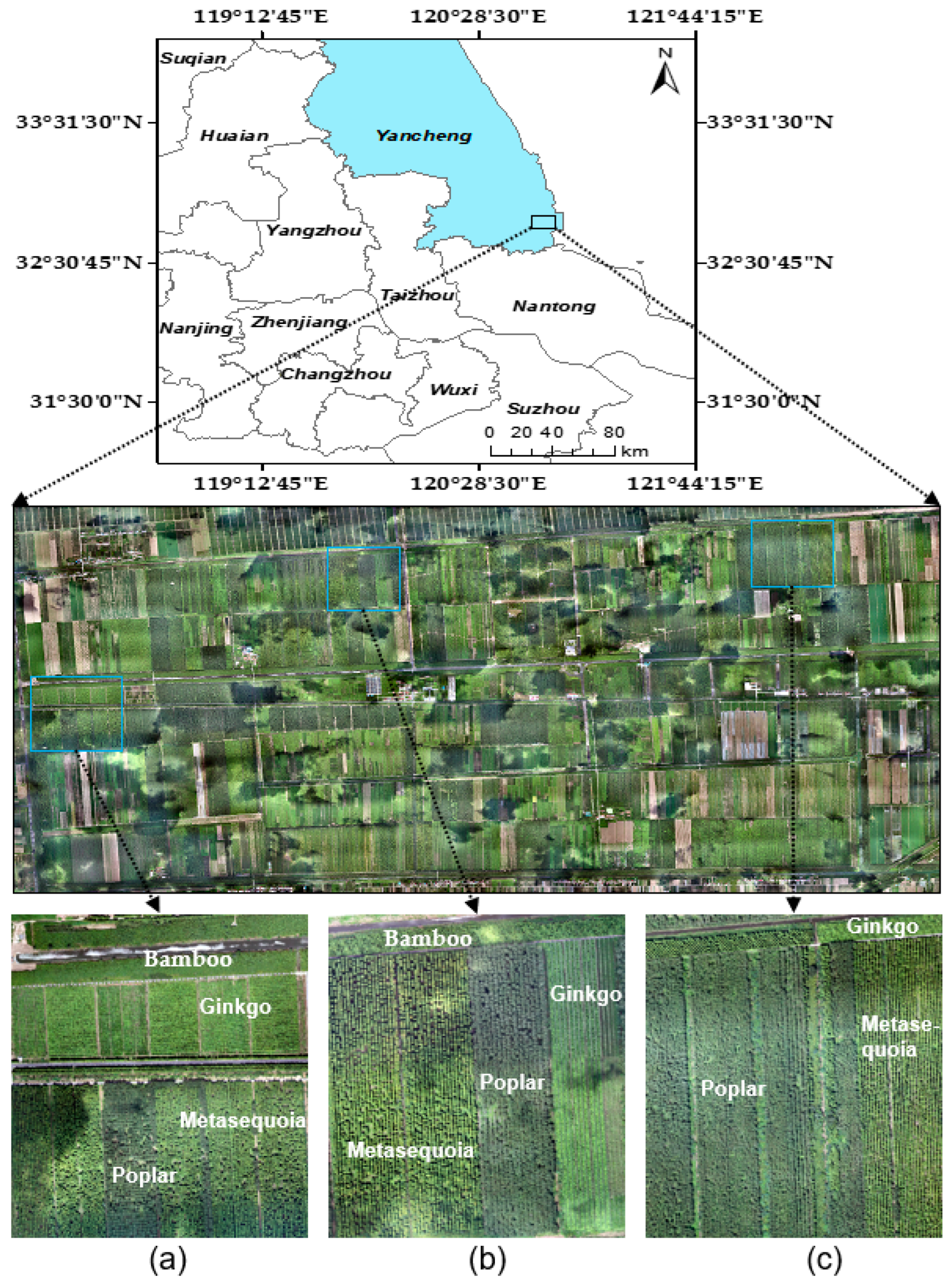
2.1. Study Area
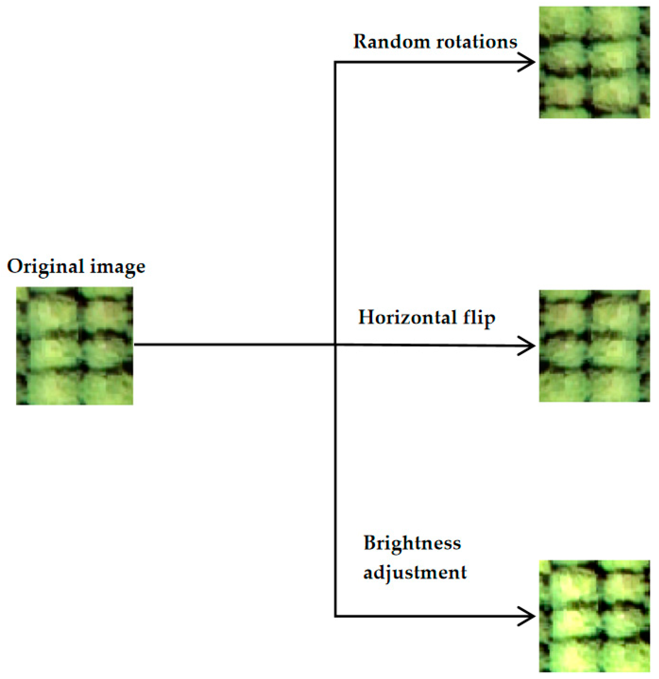
2.2. Data Collection and Preprocessing
3. Methodology
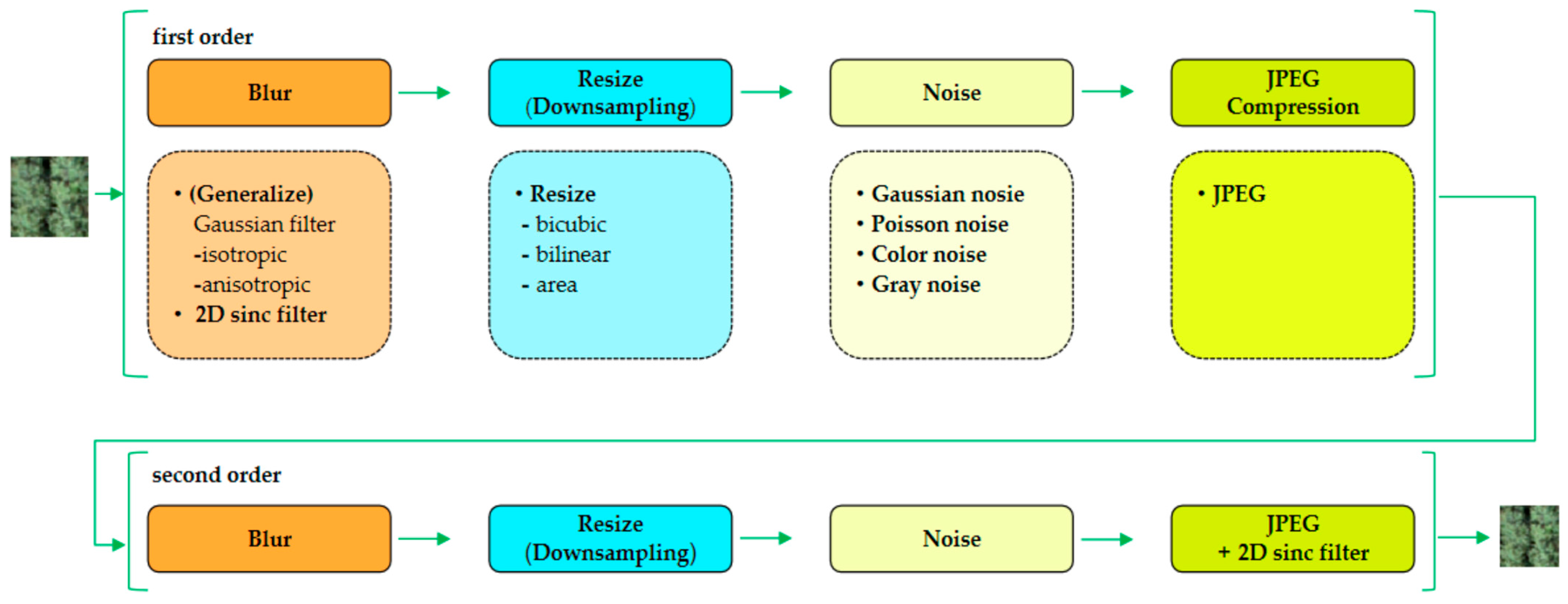
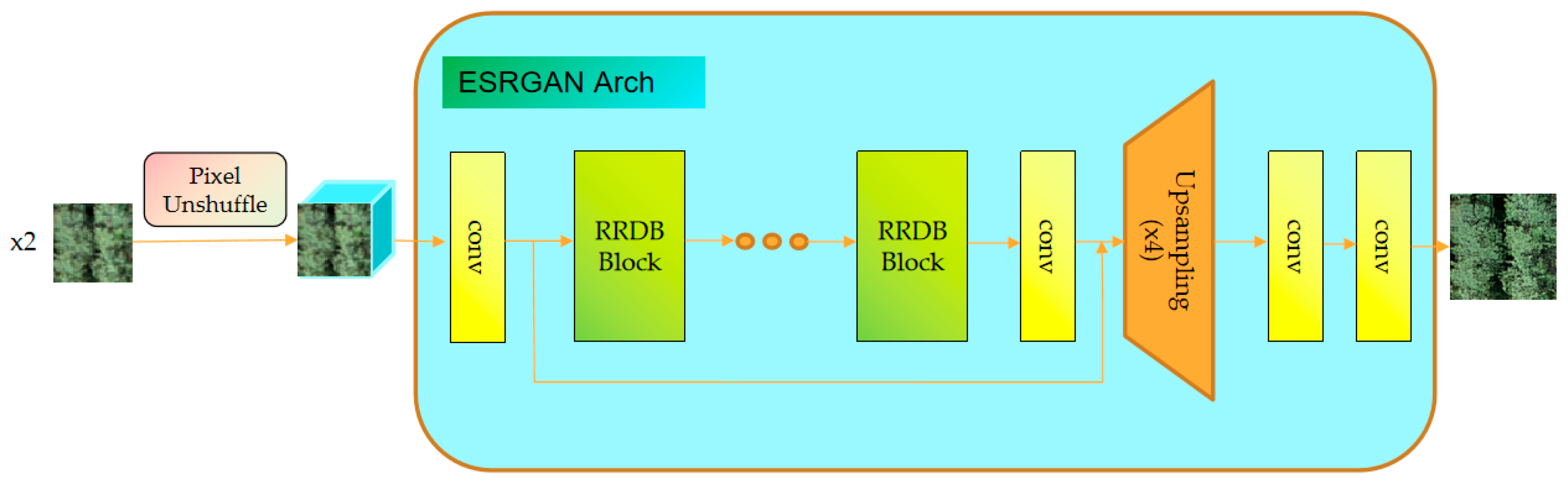
3.1. Super-Resolution Reconstruction
3.2. Model Training
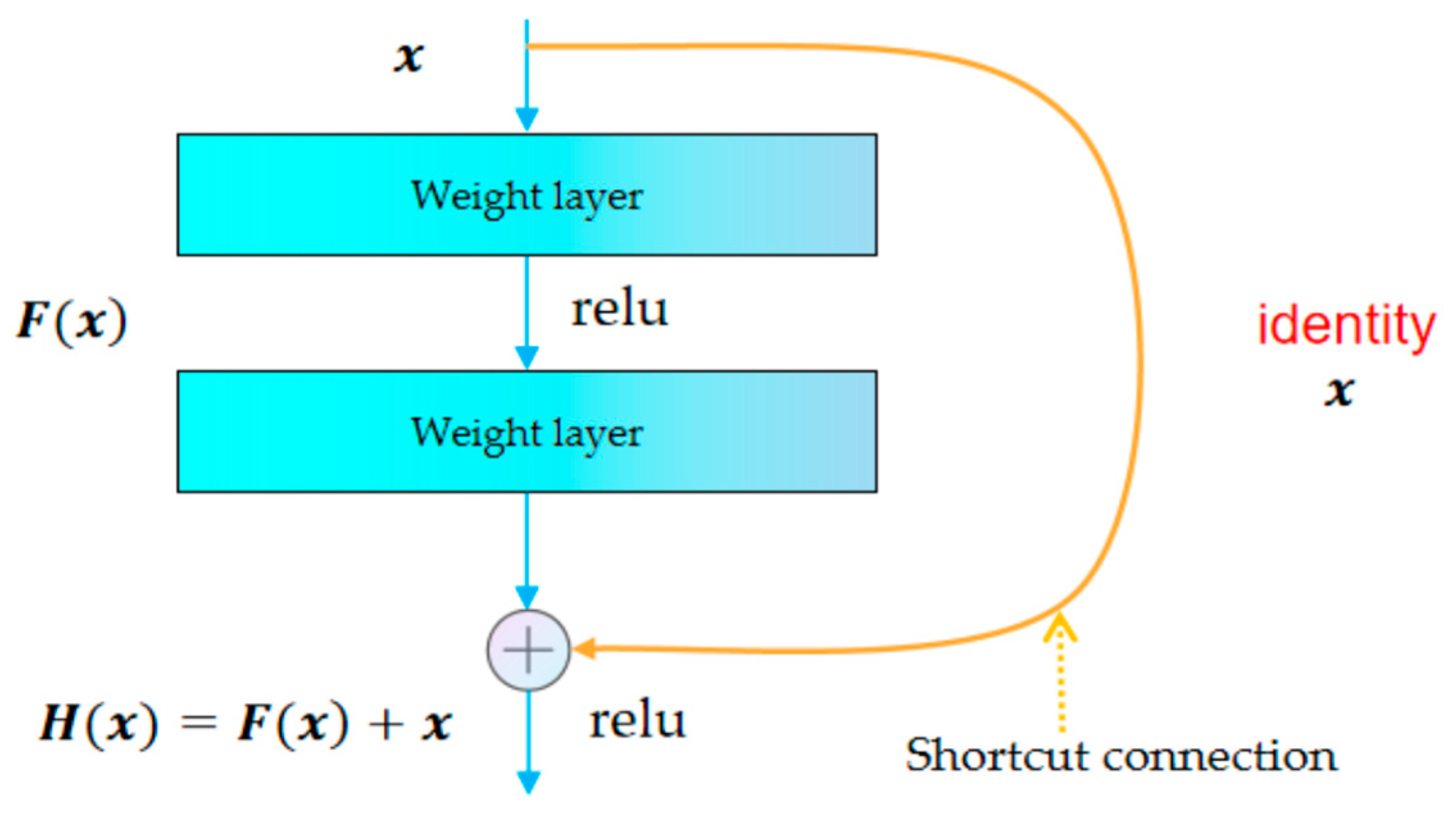
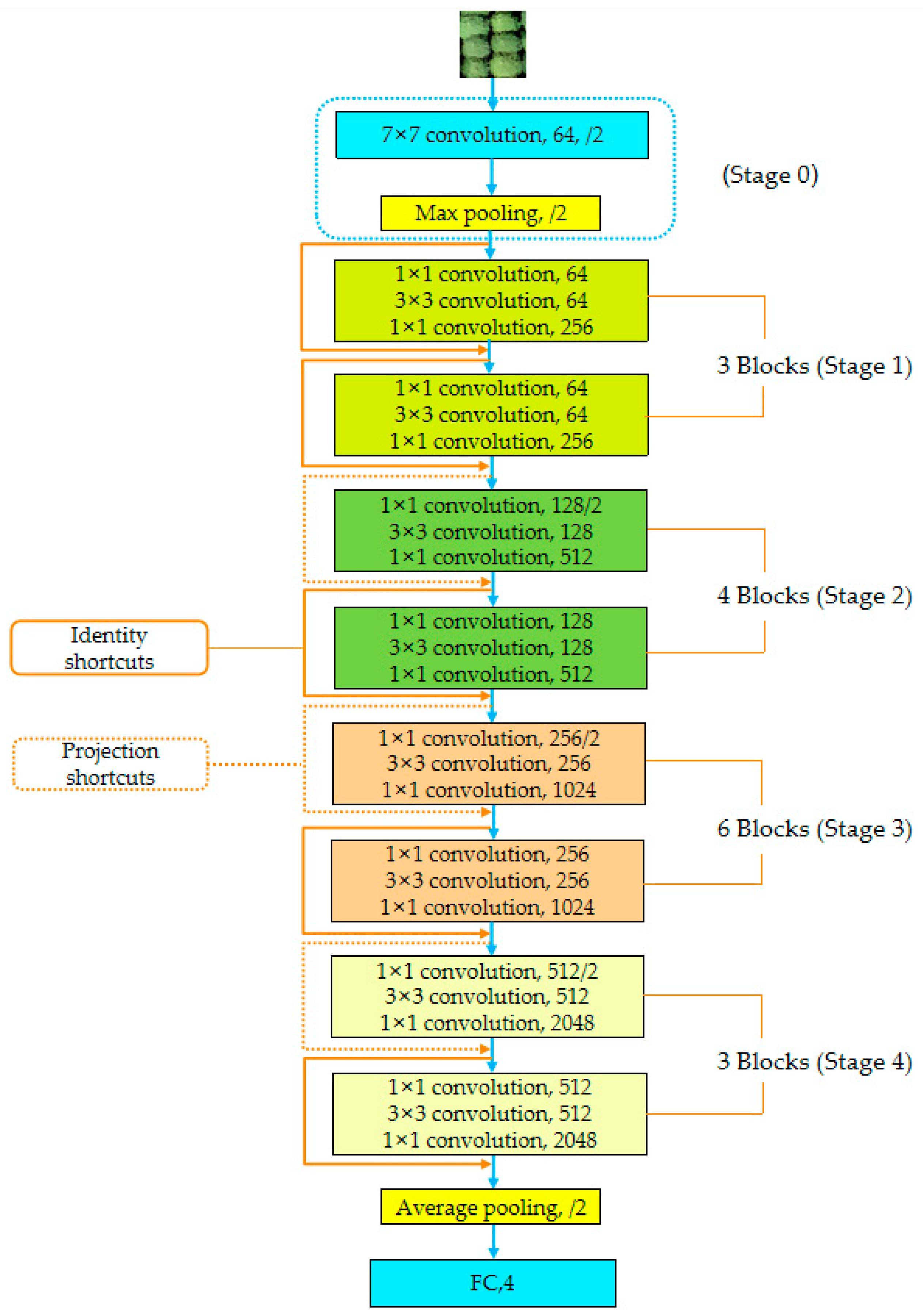
3.2.1. ResNet Model
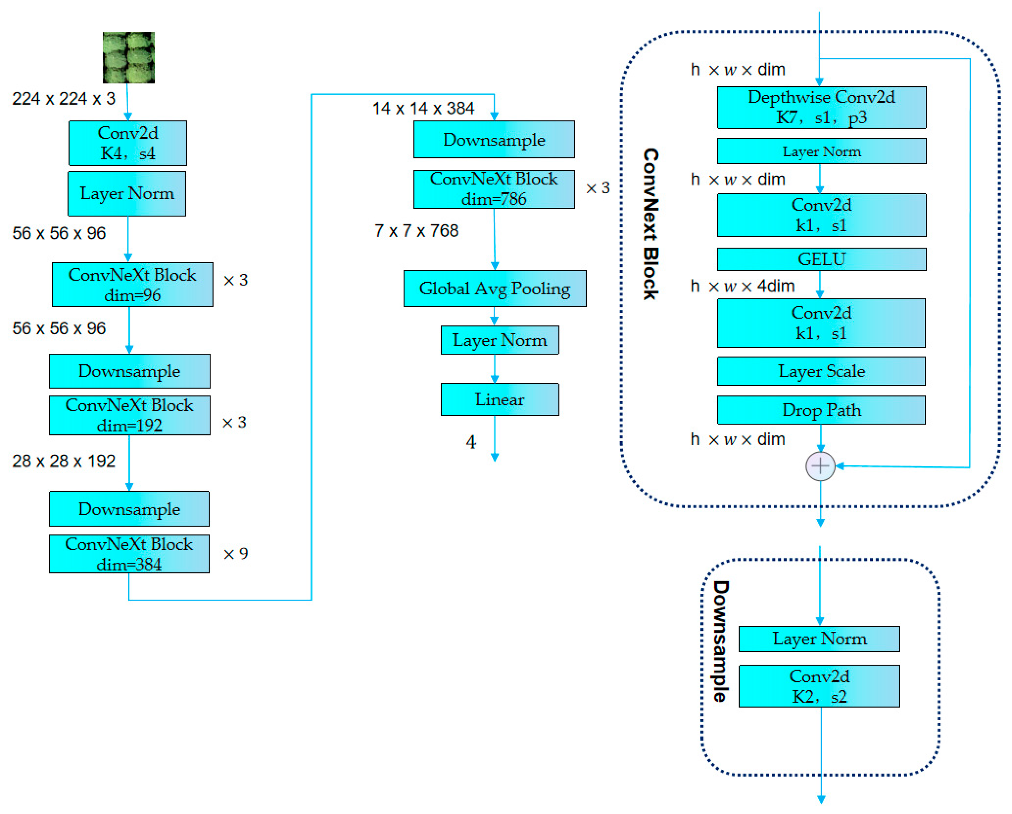
3.2.2. ConvNeXt Model
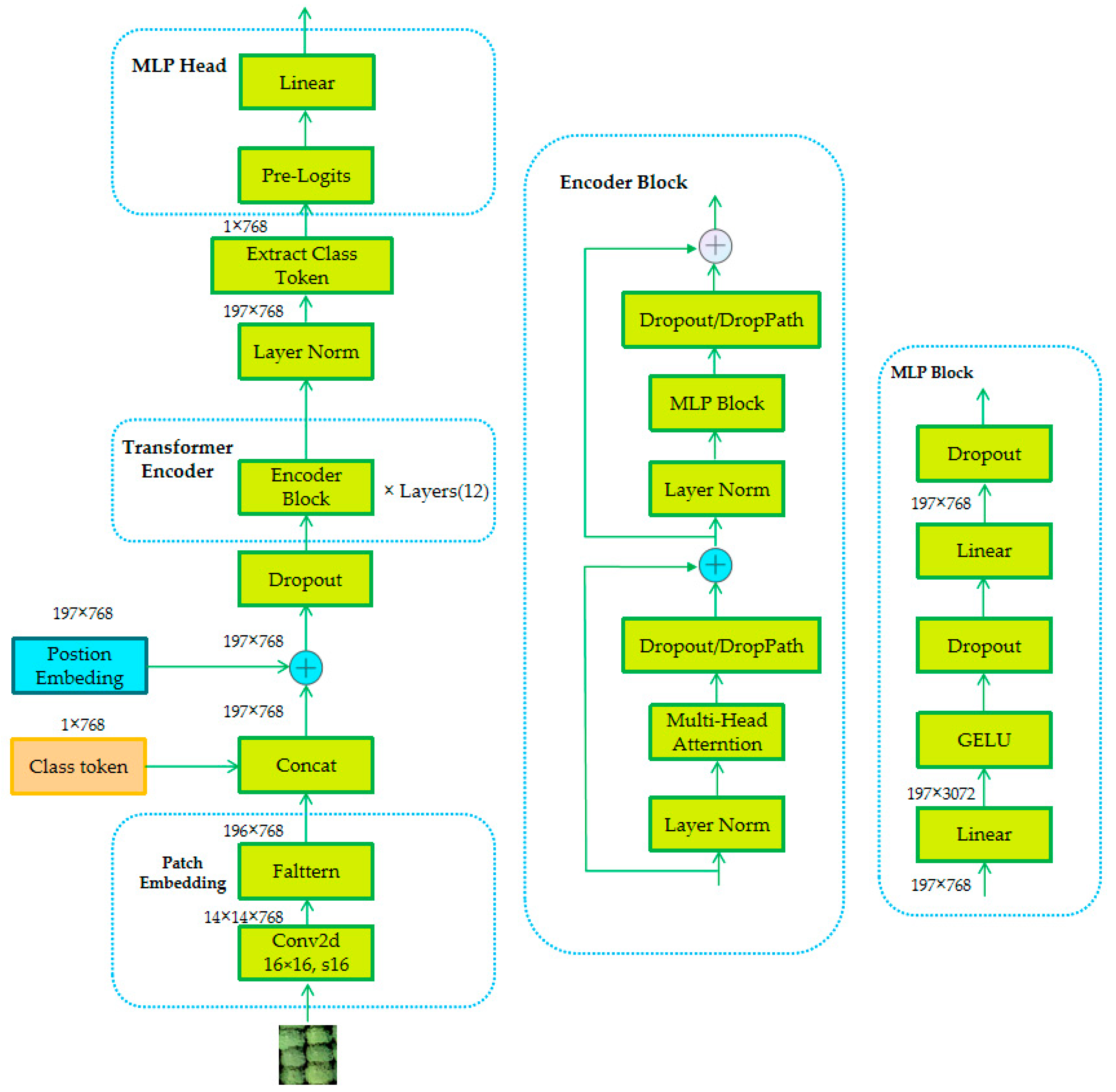
3.2.3. ViT Model
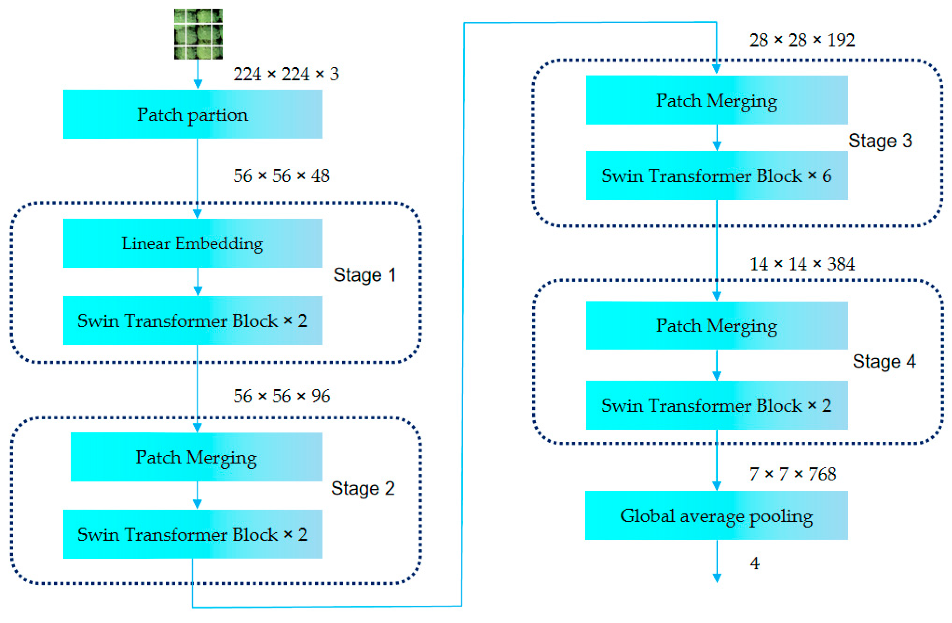
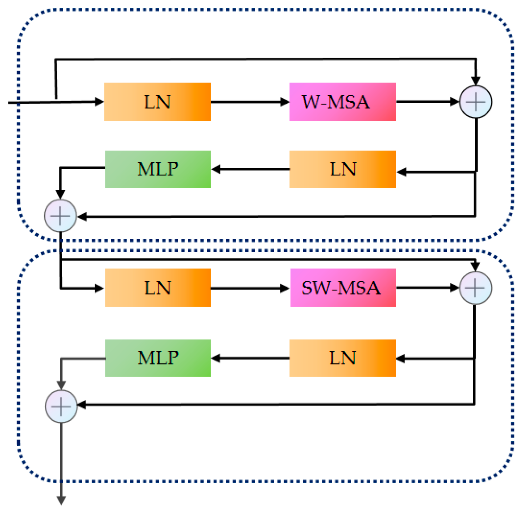
3.2.4. Swin Transformer Model
3.3. Experimental Environment
4. Results
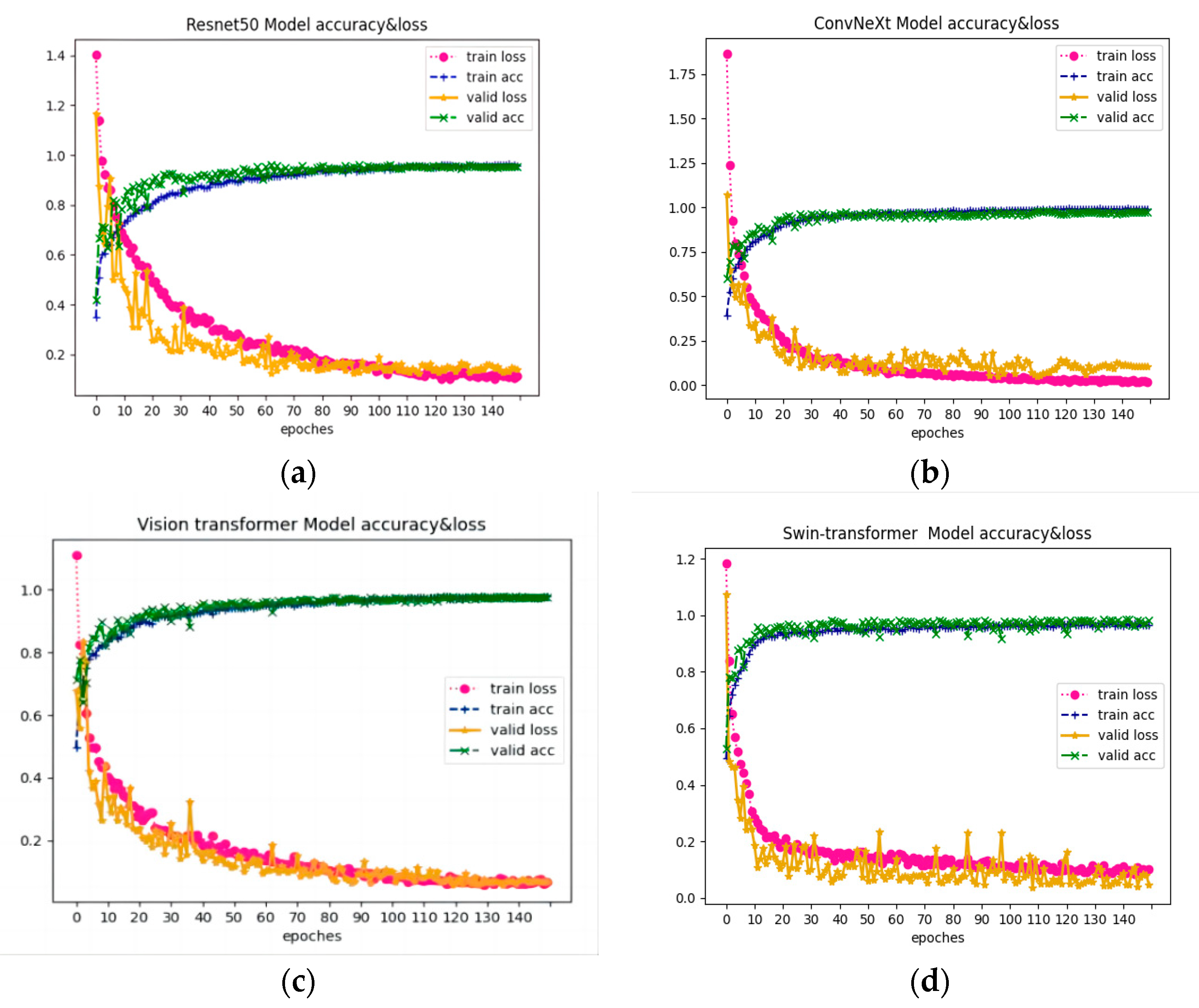
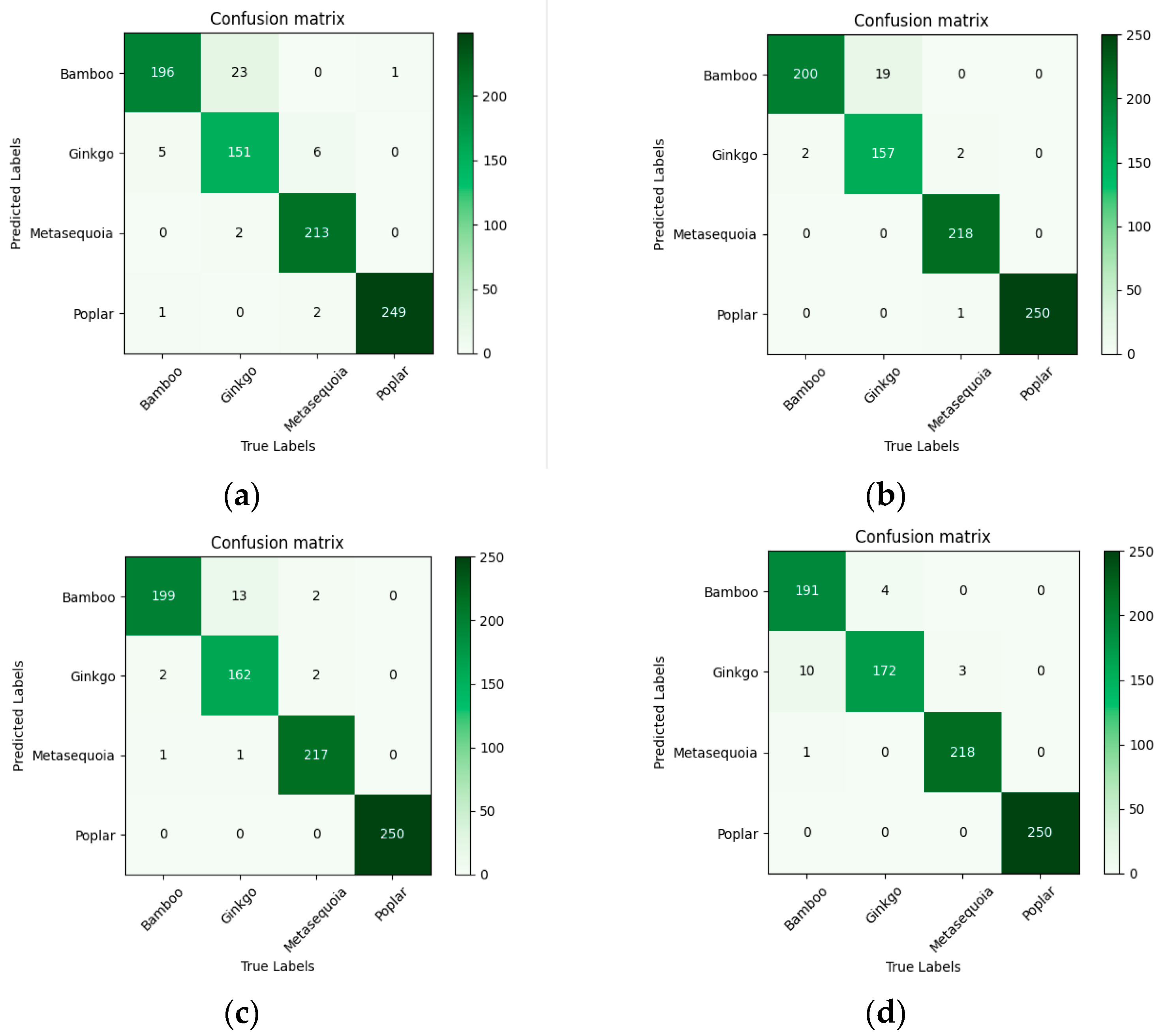
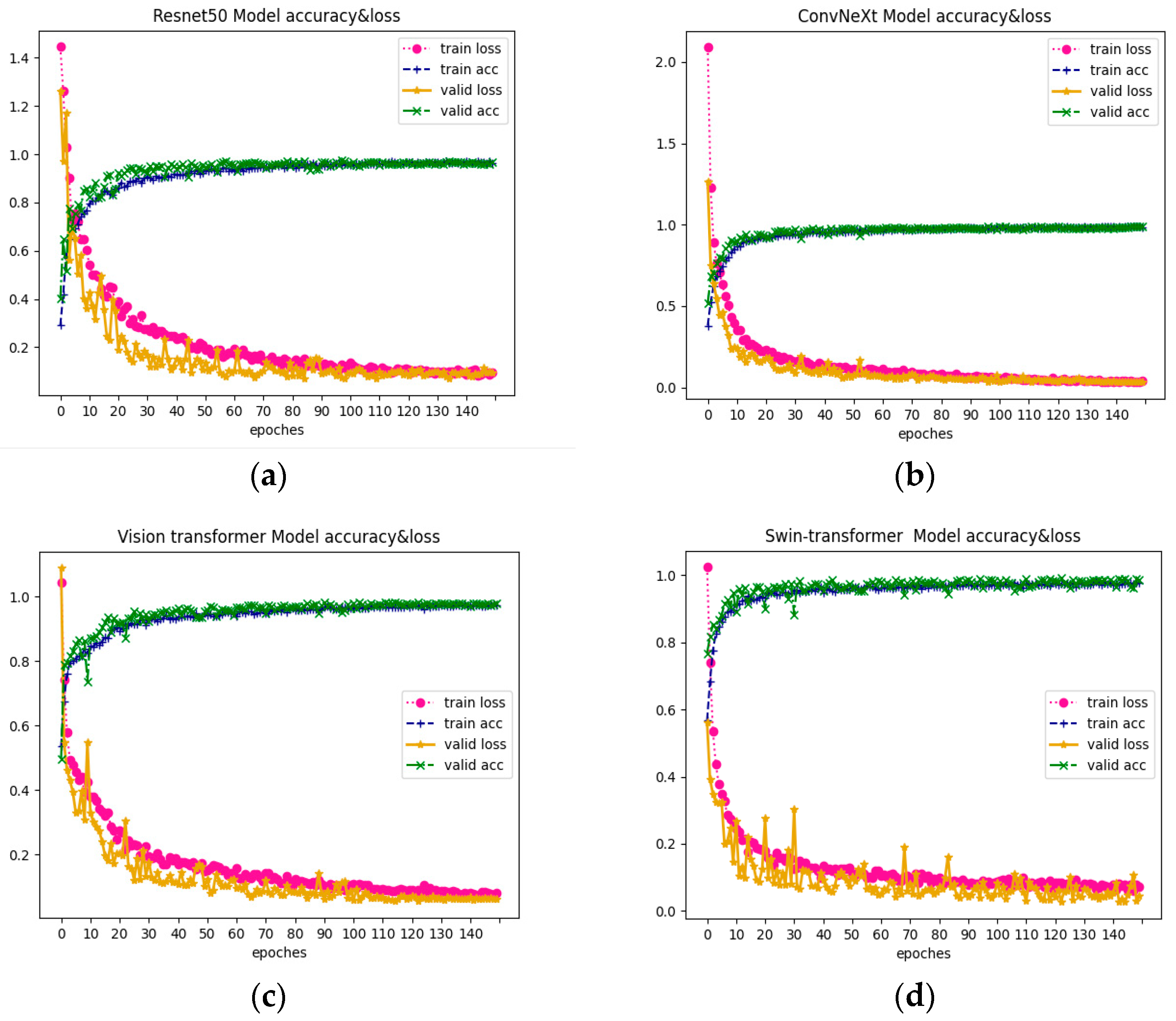
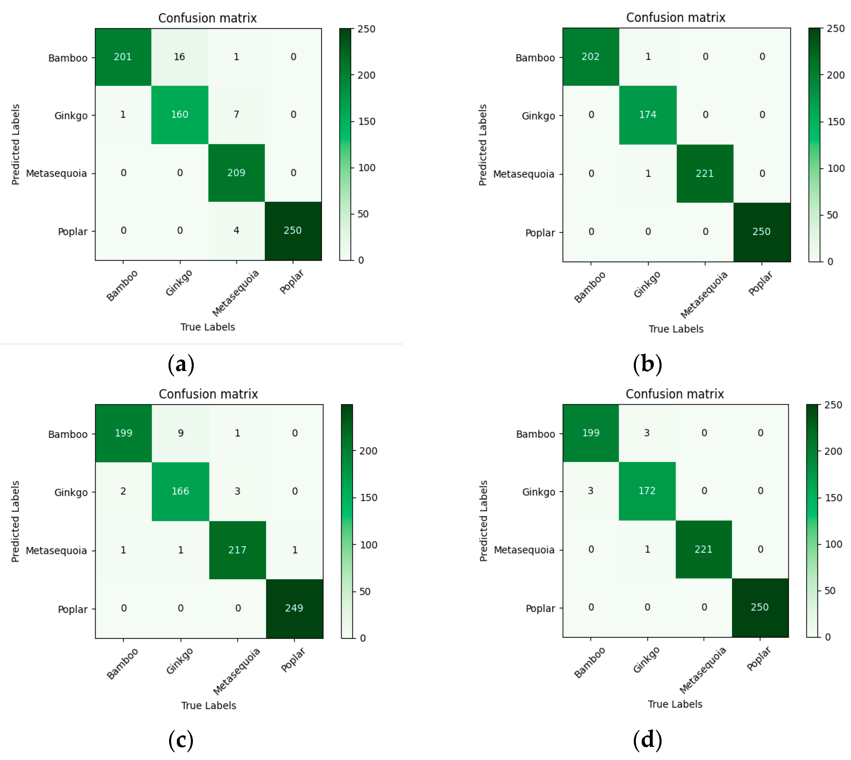
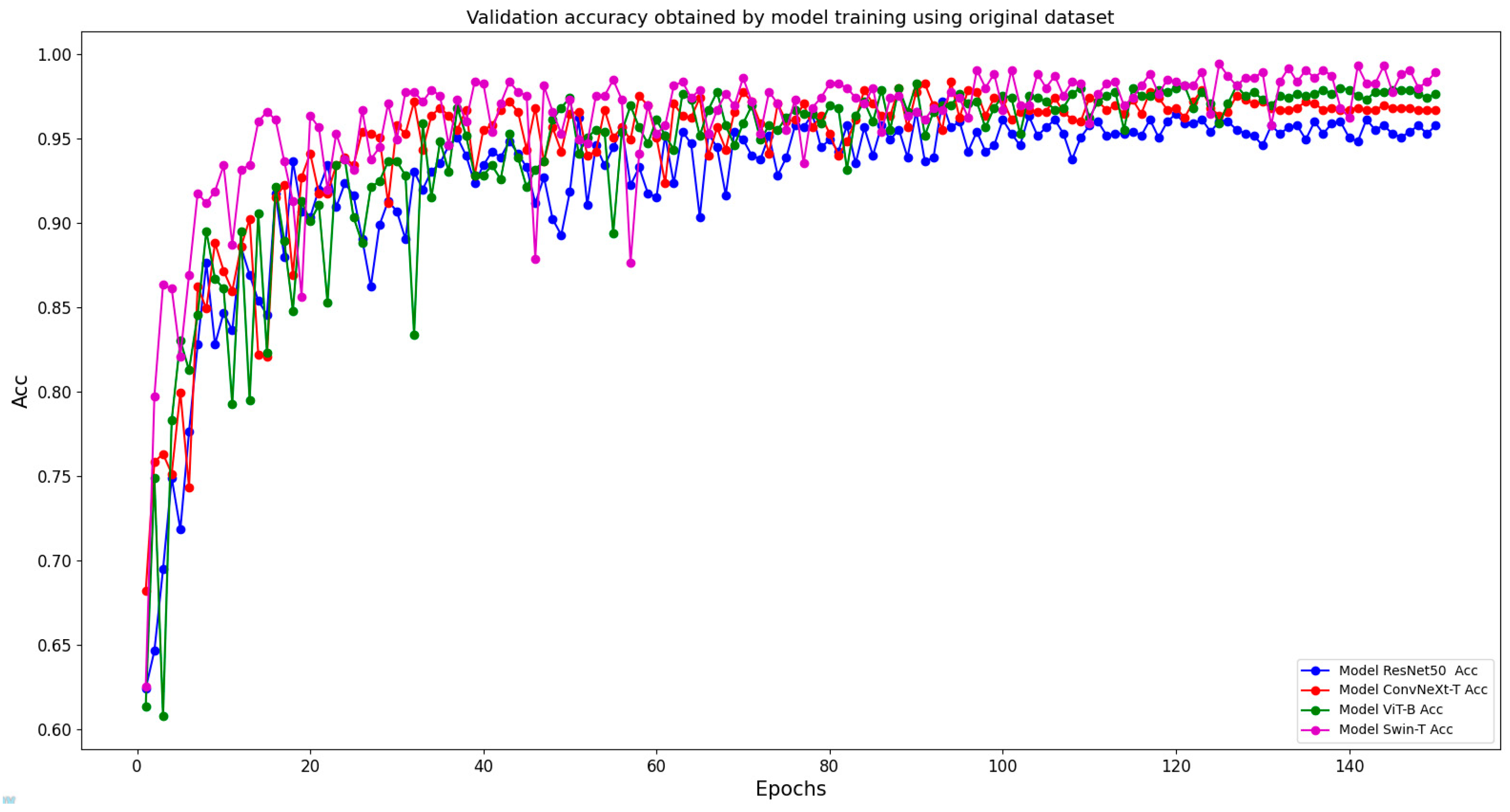
4.1. Comparison of CNN and Transformer Models for Tree Species Classification
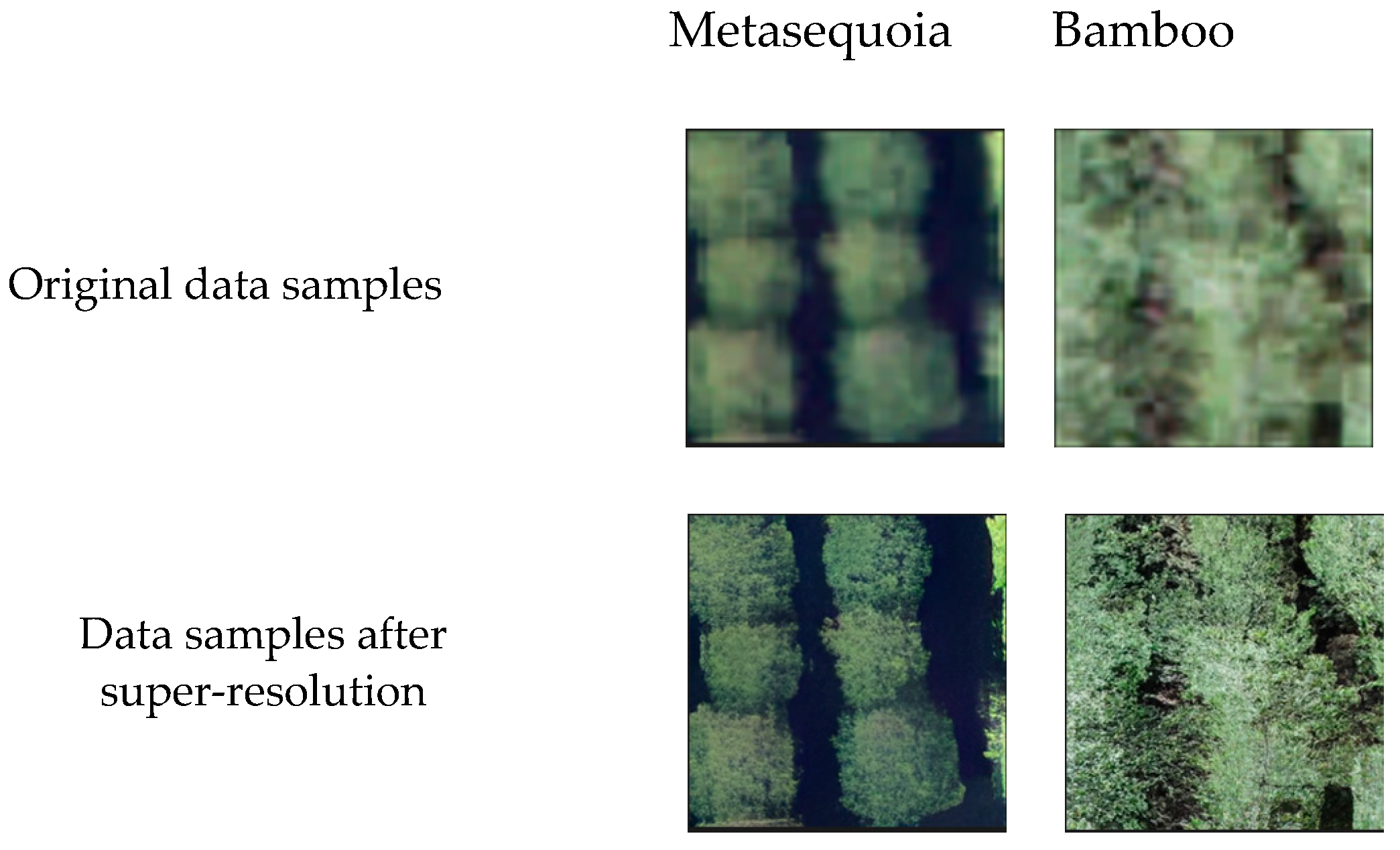
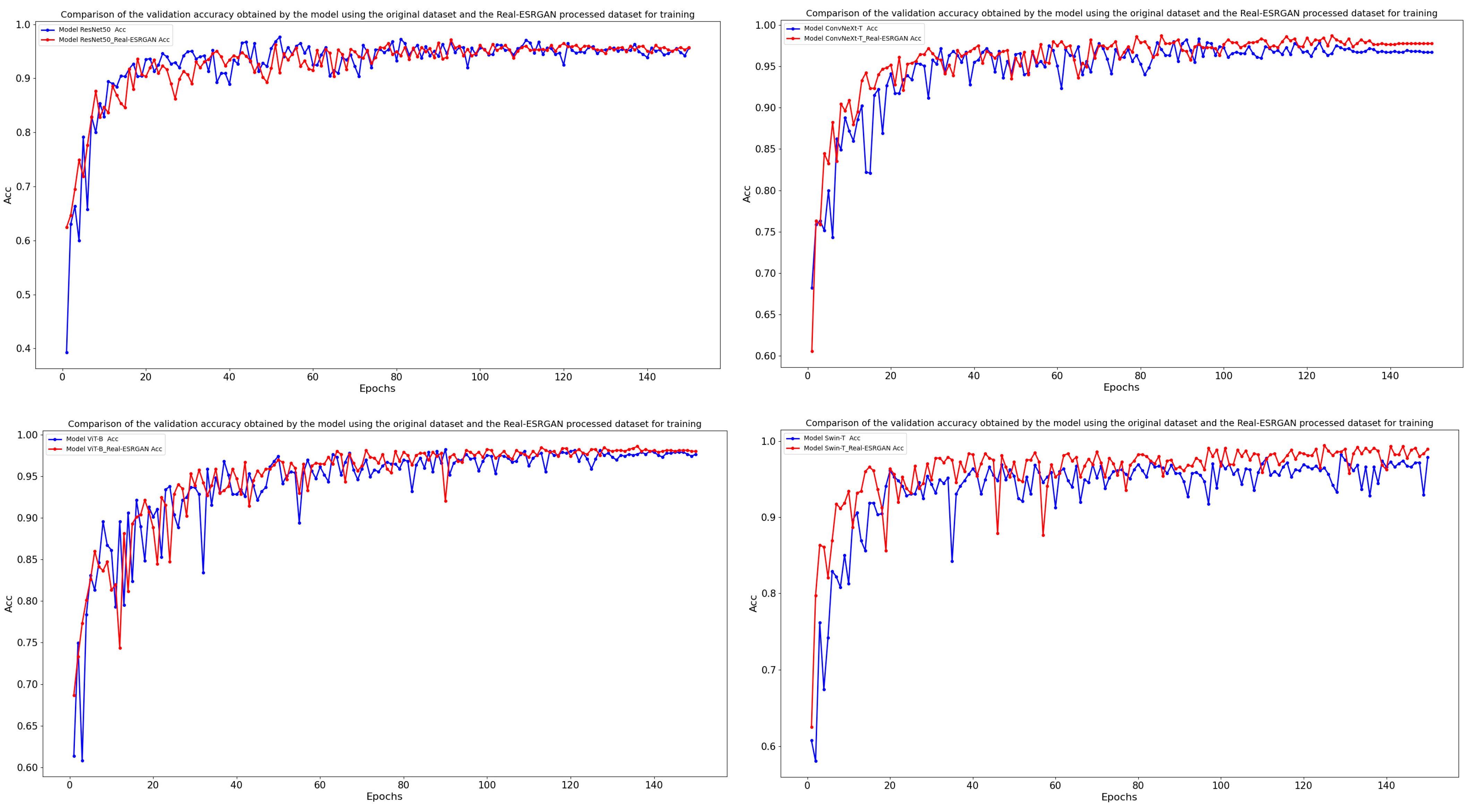
4.2. Super-Resolution Reconstruction for Improved Tree Species Classification
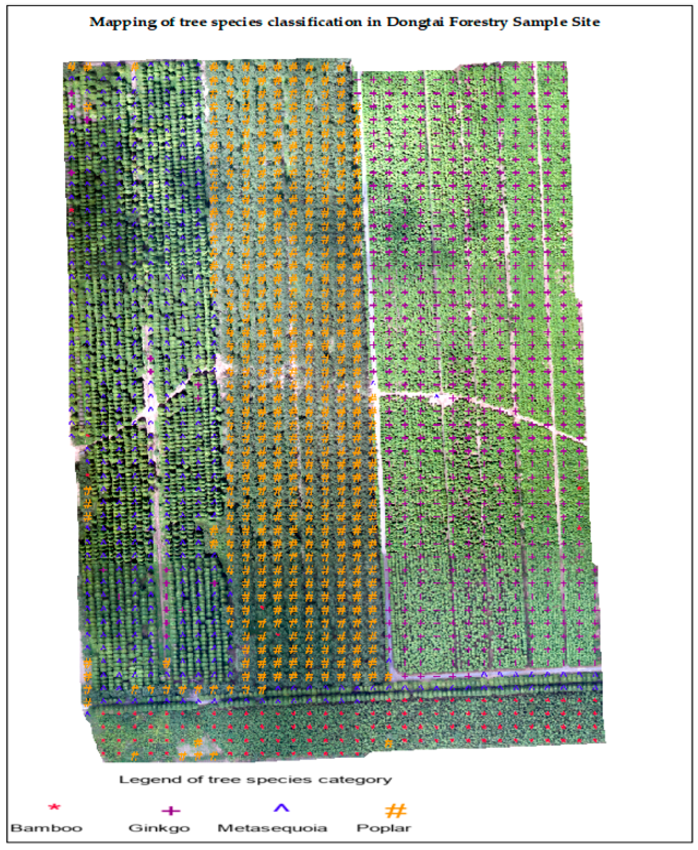
4.3. Distribution Map of Tree Species in Dongtai Forest Plot
5. Discussion
5.1. Performance of CNN and Transformer in Classifying Tree Species Using the Original Dataset
5.2. Performance of CNN and Transformer in Tree Species Classification Using Super-Resolution Reconstructed Dataset
6. Conclusions
Author Contributions
Funding
Data Availability Statement
Acknowledgments
Conflicts of Interest
References
- Zhao, D.; Pang, Y.; Liu, L.; Li, Z. Individual tree classification using airborne LiDAR and hyperspectral data in a natural mixed forest of northeast China. Forests 2020, 11, 303. [Google Scholar] [CrossRef] [Green Version]
- Marrs, J.; Ni-Meister, W. Machine learning techniques for tree species classification using co-registered LiDAR and hyperspectral data. Remote Sens. 2019, 11, 819. [Google Scholar] [CrossRef] [Green Version]
- Ballanti, L.; Blesius, L.; Hines, E.; Kruse, B. Tree species classification using hyperspectral imagery: A comparison of two classifiers. Remote Sens. 2016, 8, 445. [Google Scholar] [CrossRef] [Green Version]
- Sun, Y.; Xin, Q.; Huang, J.; Huang, B.; Zhang, H. Characterizing tree species of a tropical wetland in southern china at the individual tree level based on convolutional neural network. IEEE J. Sel. Top. Appl. Earth Obs. Remote Sens. 2019, 12, 4415–4425. [Google Scholar] [CrossRef]
- Heikkinen, V.; Tokola, T.; Parkkinen, J.; Korpela, I.; Jaaskelainen, T. Simulated multispectral imagery for tree species classification using support vector machines. IEEE Trans. Geosci. Remote Sens. 2009, 48, 1355–1364. [Google Scholar] [CrossRef]
- Zhang, Z.; Liu, X. Support vector machines for tree species identification using LiDAR-derived structure and intensity variables. Geocarto Int. 2013, 28, 364–378. [Google Scholar] [CrossRef]
- Ab Majid, I.; Abd Latif, Z.; Adnan, N.A. Tree species classification using worldview-3 data. In Proceedings of the 2016 7th IEEE Control and System Graduate Research Colloquium (ICSGRC), Shah Alam, Malaysia, 8 August 2016; pp. 73–76. [Google Scholar] [CrossRef]
- Bondarenko, A.; Aleksejeva, L.; Jumutc, V.; Borisov, A. Classification tree extraction from trained artificial neural networks. Procedia Comput. Sci. 2017, 104, 556–563. [Google Scholar] [CrossRef]
- Raczko, E.; Zagajewski, B. Tree species classification of the UNESCO man and the biosphere Karkonoski National Park (Poland) using artificial neural networks and APEX hyperspectral images. Remote Sens. 2018, 10, 1111. [Google Scholar] [CrossRef] [Green Version]
- Karlson, M.; Ostwald, M.; Reese, H.; Bazié, H.R.; Tankoano, B. Assessing the potential of multi-seasonal WorldView-2 imagery for mapping West African agroforestry tree species. Int. J. Appl. Earth Obs. Geoinf. 2016, 50, 80–88. [Google Scholar] [CrossRef]
- Immitzer, M.; Atzberger, C.; Koukal, T. Tree species classification with random forest using very high spatial resolution 8-band WorldView-2 satellite data. Remote Sens. 2012, 4, 2661–2693. [Google Scholar] [CrossRef] [Green Version]
- Hologa, R.; Scheffczyk, K.; Dreiser, C.; Gärtner, S. Tree species classification in a temperate mixed mountain forest landscape using random forest and multiple datasets. Remote Sens. 2021, 13, 4657. [Google Scholar] [CrossRef]
- Burai, P.; Beko, L.; Lenart, C.; Tomor, T. Classification of energy tree species using support vector machines. In Proceedings of the 2014 6th Workshop on Hyperspectral Image and Signal Processing: Evolution in Remote Sensing (WHISPERS), Lausanne, Switzerland, 24–27 June 2014; pp. 1–4. [Google Scholar] [CrossRef]
- da Rocha, S.J.S.S.; Torres, C.M.M.E.; Jacovine, L.A.G.; Leite, H.G.; Gelcer, E.M.; Neves, K.M.; Schettini, B.L.S.; Villanova, P.H.; da Silva, L.F.; Reis, L.P. Artificial neural networks: Modeling tree survival and mortality in the Atlantic Forest biome in Brazil. Sci. Total Environ. 2018, 645, 655–661. [Google Scholar] [CrossRef] [PubMed]
- Freeman, E.A.; Moisen, G.G.; Frescino, T.S. Evaluating effectiveness of down-sampling for stratified designs and unbalanced prevalence in Random Forest models of tree species distributions in Nevada. Ecol. Model. 2012, 233, 1–10. [Google Scholar] [CrossRef]
- LeCun, Y.; Bottou, L.; Bengio, Y.; Haffner, P. Gradient-based learning applied to document recognition. Proc. IEEE 1998, 86, 2278–2324. [Google Scholar] [CrossRef] [Green Version]
- Krizhevsky, A.; Sutskever, I.; Hinton, G.E. Imagenet classification with deep convolutional neural networks. Commun. ACM 2017, 60, 84–90. [Google Scholar] [CrossRef] [Green Version]
- Ling, C.; Jia, J.; Haiqing, W. An overview of applying high resolution remote sensing to natural resources survey. Remote Sens. Nat. Resour. 2019, 31, 1–7. [Google Scholar]
- Nezami, S.; Khoramshahi, E.; Nevalainen, O.; Pölönen, I.; Honkavaara, E. Tree species classification of drone hyperspectral and RGB imagery with deep learning convolutional neural networks. Remote Sens. 2020, 12, 1070. [Google Scholar] [CrossRef] [Green Version]
- Kapil, R.; Marvasti-Zadeh, S.M.; Goodsman, D.; Ray, N.; Erbilgin, N. Classification of Bark Beetle-Induced Forest Tree Mortality using Deep Learning. arXiv 2022, arXiv:2207.07241. [Google Scholar] [CrossRef]
- Hu, M.; Fen, H.; Yang, Y.; Xia, K.; Ren, L. Tree species identification based on the fusion of multiple deep learning models transfer learning. In Proceedings of the 2018 Chinese Automation Congress (CAC), Xi’an, China, 30 November–2 December 2018; pp. 2135–2140. [Google Scholar] [CrossRef]
- Natesan, S.; Armenakis, C.; Vepakomma, U. Individual tree species identification using Dense Convolutional Network (DenseNet) on multitemporal RGB images from UAV. J. Unmanned Veh. Syst. 2020, 8, 310–333. [Google Scholar] [CrossRef]
- Ford, D.J. UAV Imagery for Tree Species Classification in Hawai’i: A Comparison of MLC, RF, and CNN Supervised Classification. Ph.D. Thesis, University of Hawai’i at Manoa, Honolulu, HI, USA, 2020. [Google Scholar]
- Chen, X.; Jiang, K.; Zhu, Y.; Wang, X.; Yun, T. Individual tree crown segmentation directly from UAV-borne LiDAR data using the PointNet of deep learning. Forests 2021, 12, 131. [Google Scholar] [CrossRef]
- Wang, X.; Xie, L.; Dong, C.; Shan, Y. Real-esrgan: Training real-world blind super-resolution with pure synthetic data. In Proceedings of the IEEE/CVF International Conference on Computer Vision, Virtual, 11–17 October 2021; pp. 1905–1914. [Google Scholar]
- Wang, X.; Yu, K.; Wu, S.; Gu, J.; Liu, Y.; Dong, C.; Qiao, Y.; Loy, C.C. ESRGAN: Enhanced Super-Resolution Generative Adversarial Networks. In Proceedings of the European Conference on Computer Vision (ECCV) 2018, Munich, Germany, 8–14 September 2018; pp. 63–79. [Google Scholar] [CrossRef] [Green Version]
- Schonfeld, E.; Schiele, B.; Khoreva, A. A u-net based discriminator for generative adversarial networks. In Proceedings of the IEEE/CVF Conference on Computer Vision and Pattern Recognition, Seattle, WA, USA, 13–19 June 2020; pp. 8207–8216. [Google Scholar]
- Yan, Y.; Liu, C.; Chen, C.; Sun, X.; Jin, L.; Peng, X.; Zhou, X. Fine-grained attention and feature-sharing generative adversarial networks for single image super-resolution. IEEE Trans. Multimed. 2021, 24, 1473–1487. [Google Scholar] [CrossRef]
- He, K.; Zhang, X.; Ren, S.; Sun, J. Deep residual learning for image recognition. In Proceedings of the IEEE Conference on Computer Vision and Pattern Recognition, Las Vegas, Nevada, USA, 27–30 June 2016; pp. 770–778. [Google Scholar] [CrossRef] [Green Version]
- Liu, Z.; Mao, H.; Wu, C.Y.; Feichtenhofer, C.; Darrell, T.; Xie, S. A ConvNet for the 2020s. arXiv 2022, arXiv:2201.03545. [Google Scholar] [CrossRef]
- Vaswani, A.; Shazeer, N.; Parmar, N.; Uszkoreit, J.; Jones, L.; Gomez, A.N.; Kaiser, Ł.; Polosukhin, I. Attention is all you need. arXiv 2017, arXiv:1706.03762. [Google Scholar] [CrossRef]
- Hendrycks, D.; Gimpel, K. Gaussian error linear units (gelus). arXiv 2016, arXiv:1606.08415. [Google Scholar] [CrossRef]
- Dosovitskiy, A.; Beyer, L.; Kolesnikov, A.; Weissenborn, D.; Zhai, X.; Unterthiner, T.; Dehghani, M.; Minderer, M.; Heigold, G.; Gelly, S. An image is worth 16x16 words: Transformers for image recognition at scale. arXiv 2020, arXiv:2010.11929. [Google Scholar] [CrossRef]
- Liu, Z.; Lin, Y.; Cao, Y.; Hu, H.; Wei, Y.; Zhang, Z.; Lin, S.; Guo, B. Swin transformer: Hierarchical vision transformer using shifted windows. In Proceedings of the IEEE/CVF International Conference on Computer Vision, Virtual, 11–17 October 2021; pp. 10012–10022. [Google Scholar] [CrossRef]
- Egli, S.; Höpke, M. CNN-based tree species classification using high resolution RGB image data from automated UAV observations. Remote Sens. 2020, 12, 3892. [Google Scholar] [CrossRef]
- Reedha, R.; Dericquebourg, E.; Canals, R.; Hafiane, A. Transformer neural network for weed and crop classification of high resolution UAV images. Remote Sens. 2022, 14, 592. [Google Scholar] [CrossRef]


| Stage | Output_Size | ResNet-50 |
|---|---|---|
| Stage0 | 112 × 112 | 7 × 7, 64, stride 2 |
| Stage1 | 56 × 56 | 3 × 3 max pooling, stride 2 |
| Stage2 | 28 × 28 | |
| Stage3 | 14 × 14 | |
| Stage4 | 7 × 7 | |
| 1 × 1 | average pooling, 4-d fc, softmax |
| Layer_Name | Output_Size | ConvNeXt-T |
|---|---|---|
| Conv1 | 56 × 56 | 4 × 4, 96, stride 4 |
| Conv2_x | 56 × 56 | |
| Conv3_x | 28 × 28 | |
| Conv4_x | 14 × 14 | |
| Conv5_x | 7 × 7 | |
| 1 × 1 | global average pooling, 4-d fc |
| Stage_Name | Output_Size | Swin-T |
|---|---|---|
| Stage1 | 56 × 56 | concat 4 × 4, 96, LN |
| Stage2 | 28 × 28 | concat 2 × 2, 192, LN |
| Stage3 | 14 × 14 | concat 2 × 2, 384, LN |
| Stage4 | 7 × 7 | concat 2 × 2, 768, LN |
| 1 × 1 | global average pooling, 4-d fc |
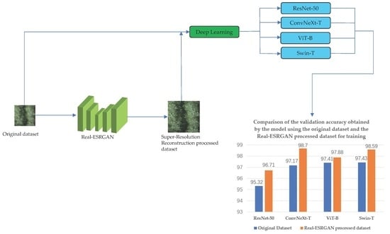
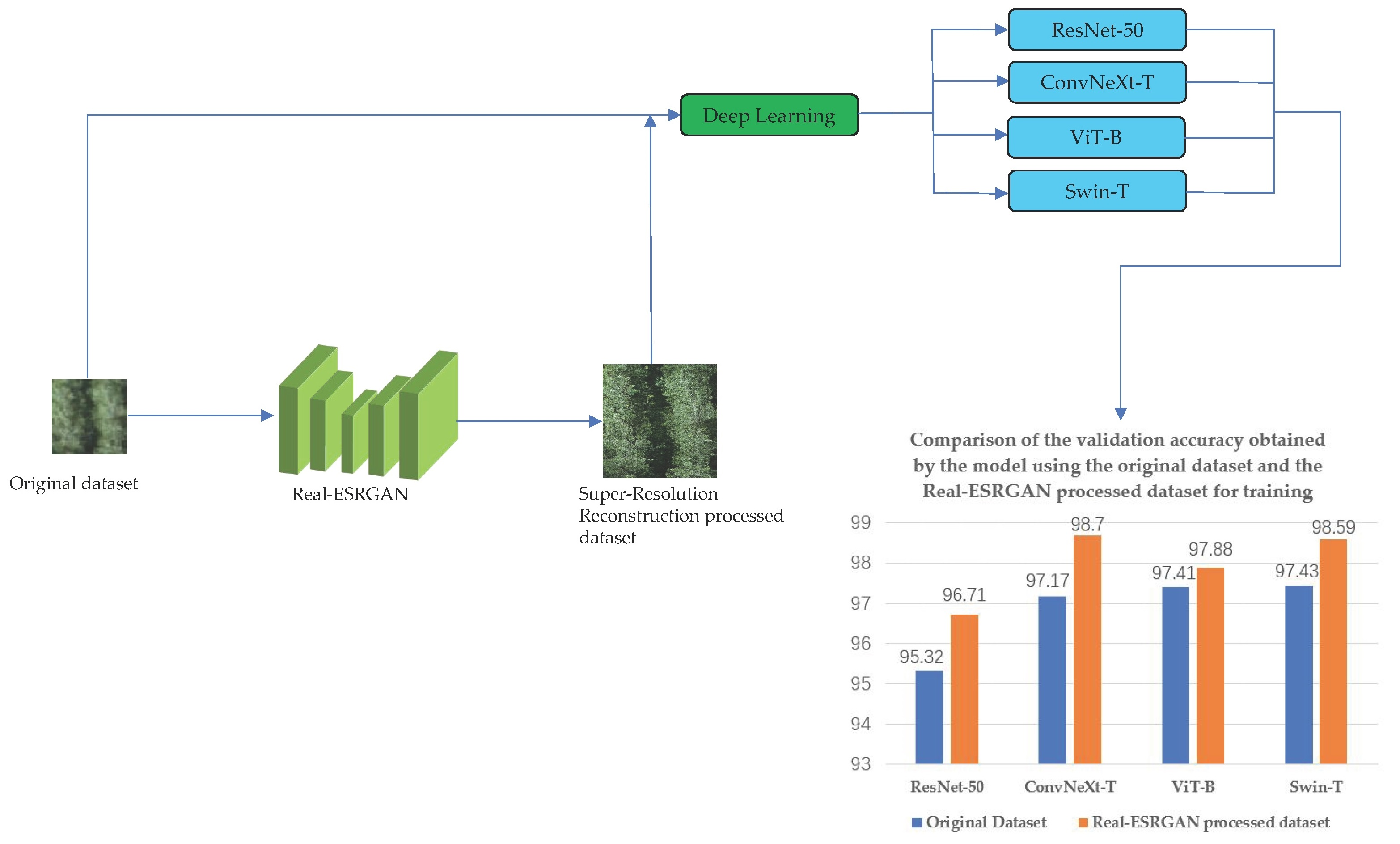
| Model | Model Size/Mb Size | Average Accuracy of Model Validation for the Original Dataset/% | Average Accuracy of Model Validation after Super-Resolution Reconstruction Restoration of the Dataset/% |
|---|---|---|---|
| ResNet-50 | 25.55 | 95.32 | 96.71 |
| ConvNeXt-T | 28.58 | 97.17 | 98.70 |
| ViT-B | 86.41 | 97.41 | 97.88 |
| Swin-T | 28.26 | 97.43 | 98.59 |
Disclaimer/Publisher’s Note: The statements, opinions and data contained in all publications are solely those of the individual author(s) and contributor(s) and not of MDPI and/or the editor(s). MDPI and/or the editor(s) disclaim responsibility for any injury to people or property resulting from any ideas, methods, instructions or products referred to in the content. |
© 2023 by the authors. Licensee MDPI, Basel, Switzerland. This article is an open access article distributed under the terms and conditions of the Creative Commons Attribution (CC BY) license (https://creativecommons.org/licenses/by/4.0/).
Share and Cite
Huang, Y.; Wen, X.; Gao, Y.; Zhang, Y.; Lin, G. Tree Species Classification in UAV Remote Sensing Images Based on Super-Resolution Reconstruction and Deep Learning. Remote Sens. 2023, 15, 2942. https://doi.org/10.3390/rs15112942
Huang Y, Wen X, Gao Y, Zhang Y, Lin G. Tree Species Classification in UAV Remote Sensing Images Based on Super-Resolution Reconstruction and Deep Learning. Remote Sensing. 2023; 15(11):2942. https://doi.org/10.3390/rs15112942
Chicago/Turabian StyleHuang, Yingkang, Xiaorong Wen, Yuanyun Gao, Yanli Zhang, and Guozhong Lin. 2023. "Tree Species Classification in UAV Remote Sensing Images Based on Super-Resolution Reconstruction and Deep Learning" Remote Sensing 15, no. 11: 2942. https://doi.org/10.3390/rs15112942