Deriving Agricultural Field Boundaries for Crop Management from Satellite Images Using Semantic Feature Pyramid Network

Abstract

We propose a Semantic Feature Pyramid Network (FPN)-based algorithm to derive agricultural field boundaries and internal non-planting regions from satellite imagery. It is aimed at providing guidance not only for land use management, but more importantly for harvest or crop protection machinery planning. The Semantic Convolutional Neural Network (CNN) FPN is first employed for pixel-wise classification on each remote sensing image, detecting agricultural parcels; a post-processing method is then developed to transfer attained pixel classification results into closed contours, as field boundaries and internal non-planting regions, including slender paths (walking or water) and obstacles (trees or electronic poles). Three study sites with different plot sizes (0.11 ha, 1.39 ha, and 2.24 ha) are selected to validate the effectiveness of our algorithm, and the performance compared with other semantic CNN (including U-Net, U-Net++, PSP-Net, and Link-Net)-based algorithms. The test results show that the crop acreage information, field boundaries, and internal non-planting area could be determined by using the proposed algorithm in different places. When the boundary number applicable for machinery planning is attained, average and total crop planting area values all remain closer to the reference ones generally when using the semantic FPN with post-processing, compared with other methods. The post-processing methodology would greatly decrease the number of inapplicable and redundant field boundaries for path planning using different CNN models. In addition, the crop planting mode and scale (especially the small-scale planting and small/blurred gap between fields) both make a great difference to the boundary delineation and crop acreage determination.

1. Introduction

Mapping the spatial distribution of agricultural parcels [1,2,3] is of great significance in land use management, administrative policy-making [4], and harvest or crop protection machinery planning [5,6]. With advances in remote sensing techniques, especially satellite imagery and the expanding availability of sensing data [7,8,9], agricultural parcel monitoring has developed rapidly and broadly in the last decade, with various applications, including large-scale yield prediction [10,11,12], crop type classifications [13,14,15], plant health monitoring [16,17,18], precision farming [19,20], etc.

Currently, considerable attention is concentrated on crop acreage determination from remote sensing data [21,22], which remains as crucial information quantifying food production at the regional or country level. It could be calculated directly from agricultural field boundaries. Traditional studies on field boundary extraction could be broadly grouped into two techniques: edge-based and region-based [23,24]. Edge-based algorithms generally seek to find field boundaries by detecting gradient changes of pixel values in map imagery, employing various filters such as Scharr, Sobel, and Canny operators. Turker et al. [25] derived sub-boundaries within agricultural fields from satellite imagery, using a canny edge detector and perceptual grouping. Yan et al. [26] presented a watershed operator-based algorithm to obtain crop field automatic extraction, from multi-temporal web-enabled landsat data. Graesser et al. [27] extracted cropland field boundaries from Landsat imagery, based on multi-scale normalization and local thresholds. Conversely, region-based studies cluster pixels into parcels based on color or textural similarity; field boundaries are then attained with delineation procedures. Segl et al. [28] detected small objects, including buildings in townships and vegetation in farmland areas, by varying the threshold values from high-resolution panchromatic satellite imagery. Da Costa et al. [29] generated vine fields from remote sensed images, in view of their textural feature versatility. García-Pedrero et al. [30] explored the agglomerative segmentation and delineation of the agricultural parcels by using an image superpixel methodology. However, boundary detection accuracy using classic methods is very constrained. For traditional edge-based algorithms, false and incomplete edges could be produced because of the over-sensitivity to high-frequency noise; region-based algorithms could be problematic due to a high dependency on the parameter selection.

With remarkable capability in learning high-level data representation, convolutional neural networks (CNNs) are widely used in image classification, object recognition, and semantic segmentation (pixel-wise classification) for various research fields and real application scenarios [31]. CNN approaches have often significantly increased detection accuracy compared to traditional/classic techniques. In the last half-decade, the application of CNNs in agricultural parcel or boundary detection is becoming an intensive research topic. For edge detection [23,32,33], Persello et al. [21] delineated agricultural fields in smallholder farms, based on the SegNet architecture and oriented watershed transform. For region detection [34,35,36], Lv et al. [37] explored the delineation and grading of actual crop production units from remote sensing imagery, using the mask region-based convolutional neural network.

The crop acreage information from boundary detection would elevate land use management and administrative policy making. Moreover, detected agricultural field boundaries could provide actionable information for harvest or crop protection operations. However, current studies on field extraction aiming at determining crop acreage for spatial analysis may yield insufficient data for agricultural machinery planning. On the one hand, the accuracy assessment of the delineated field boundaries remains almost the same as other regular object-based segmentation methods such as precision and F1; the number of the attained field boundaries applicable, inapplicable or redundant for machinery planning is not taken into account. Detected field boundaries could be highly concaved with numerous unnecessary steep corners due to mapping semantic errors, which would add great difficulty to the planning work. Moreover, the non-planting area inside those extracted segments is always ignored and unannotated. Detection of agricultural field anomaly patterns, including planter skips and waterways, is becoming increasingly important [38]. Path planning and scheduling based on given field boundaries and inner anomaly regions using different agricultural machineries, such as harvester and crop protection UAS, have been widely studied to maximize efficiency [39,40,41]. Those inner non-planting or anomaly regions, especially obstacles, would make a great difference to the overall planning of agricultural machinery.

In this article, a semantic-feature-pyramid-network-based algorithm is proposed to attain agricultural field boundary delineation, and internal non-planting region extraction from satellite images. The semantic FPN is first employed to detect agricultural parcels and field boundaries, and internal non-planting regions are then determined from those detected parcels by using the post-processing method. Besides land use management, the proposed algorithm could provide sufficient data for the planning work of the harvesters. It has been verified that the boundary numbers applicable for machinery planning, average and total crop planting area attained by using the proposed algorithms, all remain closer to the reference ones compared with others (including U-Net, U-Net++, PSP-Net, and Link-Net-based). Attained field boundaries could be improved by using the developed post-processing method. Internal non-planting areas such as slender paths (walking or water) and obstacles (trees or electronic poles) could be detected. The crop planting scale (or plot size) and planting mode would greatly affect agricultural field boundaries and internal non-planting region derivation.

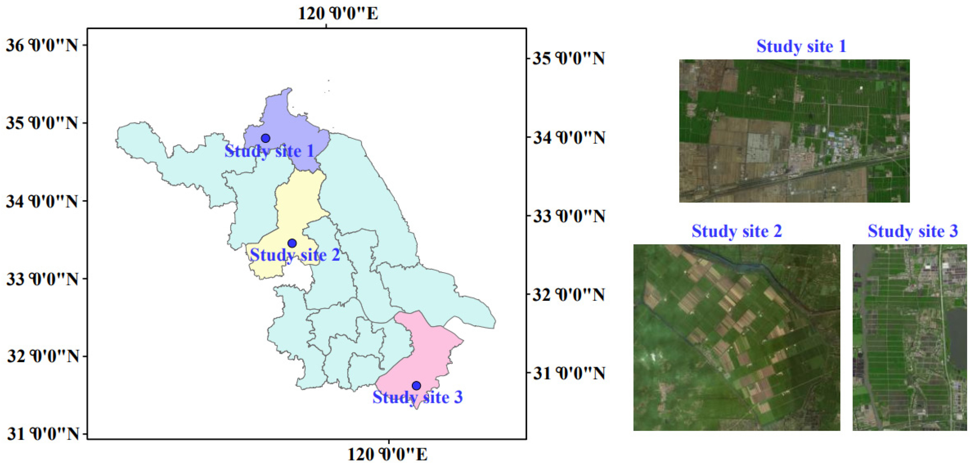
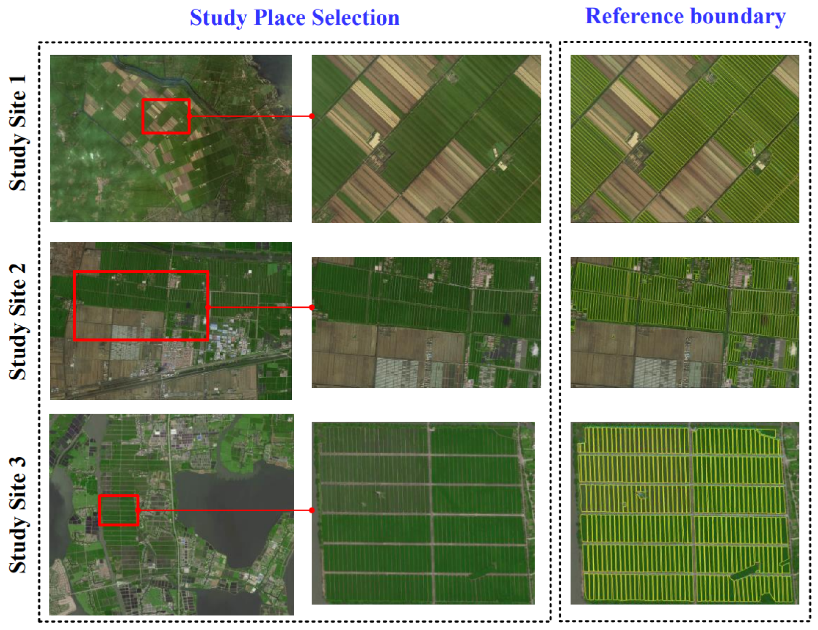
2. Study Areas and Available Datasets

Jiangsu Province is located in the Yangtze River Delta region, with a cultivated area of 45,800 square kilometers. The terrain of Jiangsu is mainly plain, with a subtropical monsoon climate, sufficient sunshine, abundant rainfall, and fertile soil, making it suitable for the cultivation of rice, wheat, rape and other crops. Rice is usually sown in mid-May, and harvested in mid-October, while wheat and rape are sown around October, and harvested in May. Besides harvest, scalable disease and pest control play a critical role in overall yield. For rice, crop protection should be carried out around August to prevent and control rice blast, false smut, sheath blight, and leaf folders, hoppers, and borers. To control rape sclerotinia sclerotiorum and wheat scab, disease and pest control work should be in progress around April. Field boundary detection and crop acreage status determination would make a great difference to the scalable management, scheduling, and planning of harvesters and grain trucks.

The experimental data are from the National Platform for Common Geospatial Information Services in China, with a map number GS-(2021)-6026. These are public data produced through both geometric and orthometric correction of aerial photographs under ‘Regulations on Management of Map Review’ and ‘Specification for Remote Sensing Image Map Production (DZ/T 0265-2014)’. To avoid the detection loss of small-plotted agricultural fields and (especially) inner non-planting areas in satellite maps, all collected imagery in the dataset is downloaded at the maximum attainable scale, with a spatial resolution of 0.5 m. Our first study site is an 8 × 5 km area of an untitled farm of rural cooperatives in Donghai County, Lianyungang City; the field average area size is close to 1.5 ha. The image was photographed on 30 August. The main crop type in the first study site is rice, with an urgent need for plant protection operations. The second study site is the Hongze Farm (20 × 14 km) in Hongze County, Huaian City; the field average area is around 2 ha. The image was photographed on 6 October. The planted rice in the second study site is in harvest. The third study site is Wujiang National Agricultural Demonstration Zone (5 × 7 km), Wujiang District, Suzhou City; the planted field is small-scale with an average area of 0.15 ha, and the gap between fields remains minimal and vague. The image was photographed on 4 April. Planted wheat and rape were in crop protection.

Our experiment covered three sites (see Figure 1) in Jiangsu Province, to validate the performance of field boundary delineation and internal non-planting region detection. The chosen three sites are well-managed agricultural farms instead of various scattered agricultural fields, in order to provide comprehensive and regular field imagery data for the adopted convolutional network training. The crop planting or management modes are different from each other in those three study sites. On the one hand, the field plot sizes are small and different, and vary from 0.15 ha to 2 ha. On the other hand, the minimum gap between adjacent fields is also different in those three study sites, changing between 0.5 m and 2 m. Given the available map with a spatial resolution of 0.5 m, the field gap between adjacent fields could be indistinct or blurred in the map imagery. This may add great difficulties to the determination of planting acreage information and field boundaries applicable for tractor planning. It should be noted that crop management or planting modes are widely adopted in the Yangtze River Delta region. This means that the proposed algorithm would provide field delineation services not only for Jiangsu Province, but also the other places in the Yangtze River Delta region, such as Shanghai City and Zhejiang Province, using satellite map imagery with similar spatial resolution.

Without available (or reference) bounding boxes for the agricultural region in each farm, we selected more than 500 satellite images of the three study areas for necessary labeling and CNN training, and over 1000 agricultural field polygons (planting and non-planting areas) were obtained. It is worth noting that well-managed and regular agricultural fields in these farms would facilitate the necessary imaging annotations and labeling work.

3. Methodology

We propose a semantic feature pyramid networks (FPN)-based algorithm to determine agricultural field boundaries and internal non-planting areas from satellite images. Semantic FPN was first employed to detect agricultural parcels; field boundary and inner non-planting regions were then delineated and detected based on the attained agricultural parcels using the proposed post-processing algorithm.

3.1. Agricultural Land (Parcels) Detection with a Fully Convolutional Network

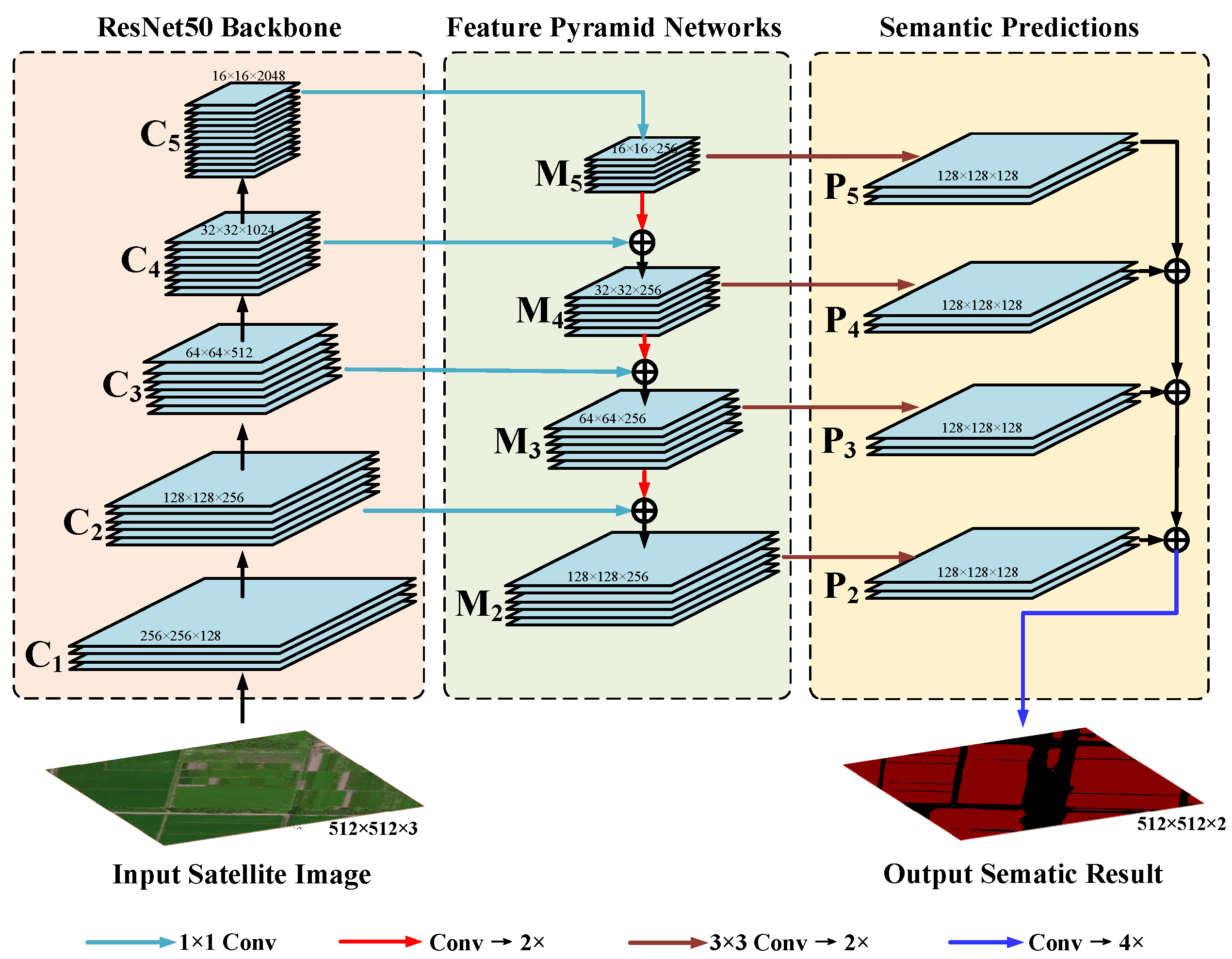
3.1.1. Network Architecture: Semantic FPN (ResNet50 Backbone)

This section was to classify the pixels in each satellite image and extract agricultural lands based on semantic or panoptic FPN [42]. The structure of the adopted semantic FPN is shown in Figure 1, which consists of three blocks mainly: bottom-up and top-down pathways, and semantic predictions. The adopted bottom-up section or backbone is topologically the same as that of the ResNet50 networks, embedded with five convolutional modules C_i (i = 1, 2, 3, 4, and 5). It is utilized to extract feature maps from sequence satellite map images while decreasing the spatial dimension and expanding the channels. FPN with four modules M_i (i = 2, 3, 4, and 5) is then employed as the top-down pathway, to increase the spatial dimensions while maintaining the channels. The top-down pathways are linked to the bottom-up ones through lateral connections, aggregating image features across the network spatially. Each module in the feature extractor (i.e., top-down pathways) outputs a prediction P_i (i = 2, 3, 4, and 5), which would be applied in the semantic logits.

As shown in Figure 2, the input satellite image size is 512 × 512 × 3. Along the bottom-up pathway of ResNet50, the resolution of C_i (i = 1, 2, 3, 4, and 5) shrinks to 256 × 256, 128 × 128, 64 × 64, 32 × 32 and 16 × 16, respectively; the channel expands to 128, 256, 512, 1024 and 2048, correspondingly. Each FPN module M_i (i = 2, 3, 4, and 5) remains the same resolution as C_i at the same level, while the channel dimension is set as 256; each module M_i is up-sampled until it reaches 128 × 128 resolution as P_i, with a fixed dimension 128. The up-sampling stage is the repeat of a 3 × 3 convolution, group norm, ReLU, and 2× bilinear up-sampling. It should be noted that the up-sampling stages differ from each other at different levels (i = 3, 4, and 5). For example, the deepest FPN module M₅ needs to perform three up-sampling stages, like P₅. The attained feature maps are then element-wise summed, followed by a 1 × 1 convolution, 4× bilinear up-sampling, and soft-max; pixel-wise class labels with 512 × 512 image resolution are finally generated.

3.1.2. Deep Supervision and Loss Function

To proceed with deep learning in the adopted Semantic FPN model, we introduce a hybrid loss function in Equation (1) which is the combination of binary cross-entropy loss and dice-coefficient loss,

$$L(Y,\stackrel{⌢}{Y})=-\frac{1}{N}{\displaystyle \sum _{b=1}^N\left(\frac{1}{2}\cdot Y_b\cdot \log {\stackrel{⌢}{Y}}_b+\frac{2\cdot Y_b\cdot {\stackrel{⌢}{Y}}_b}{Y_b+{\stackrel{⌢}{Y}}_b}\right)},$$

(1)

where Y_b is the flatten predicted probability of the b-th image, while ${\stackrel{⌢}{Y}}_b$ refers to the ground truth of the corresponding one; N denotes the pixel number of one training batch.

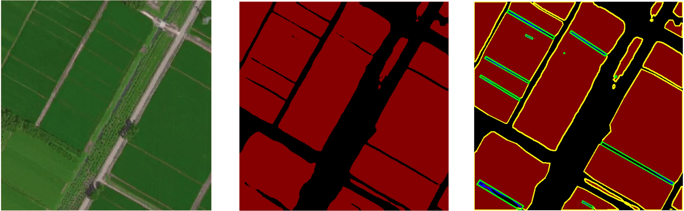
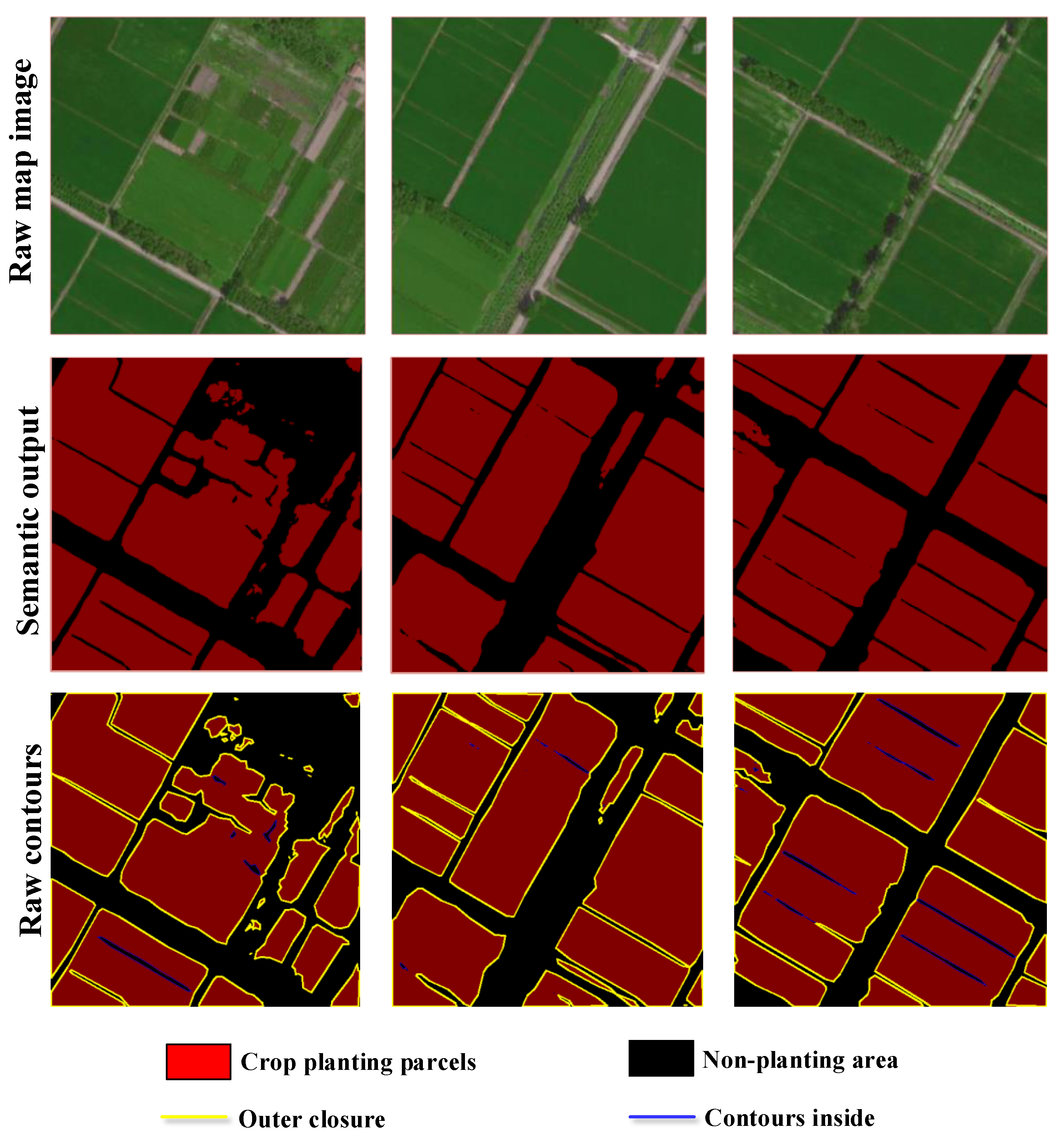
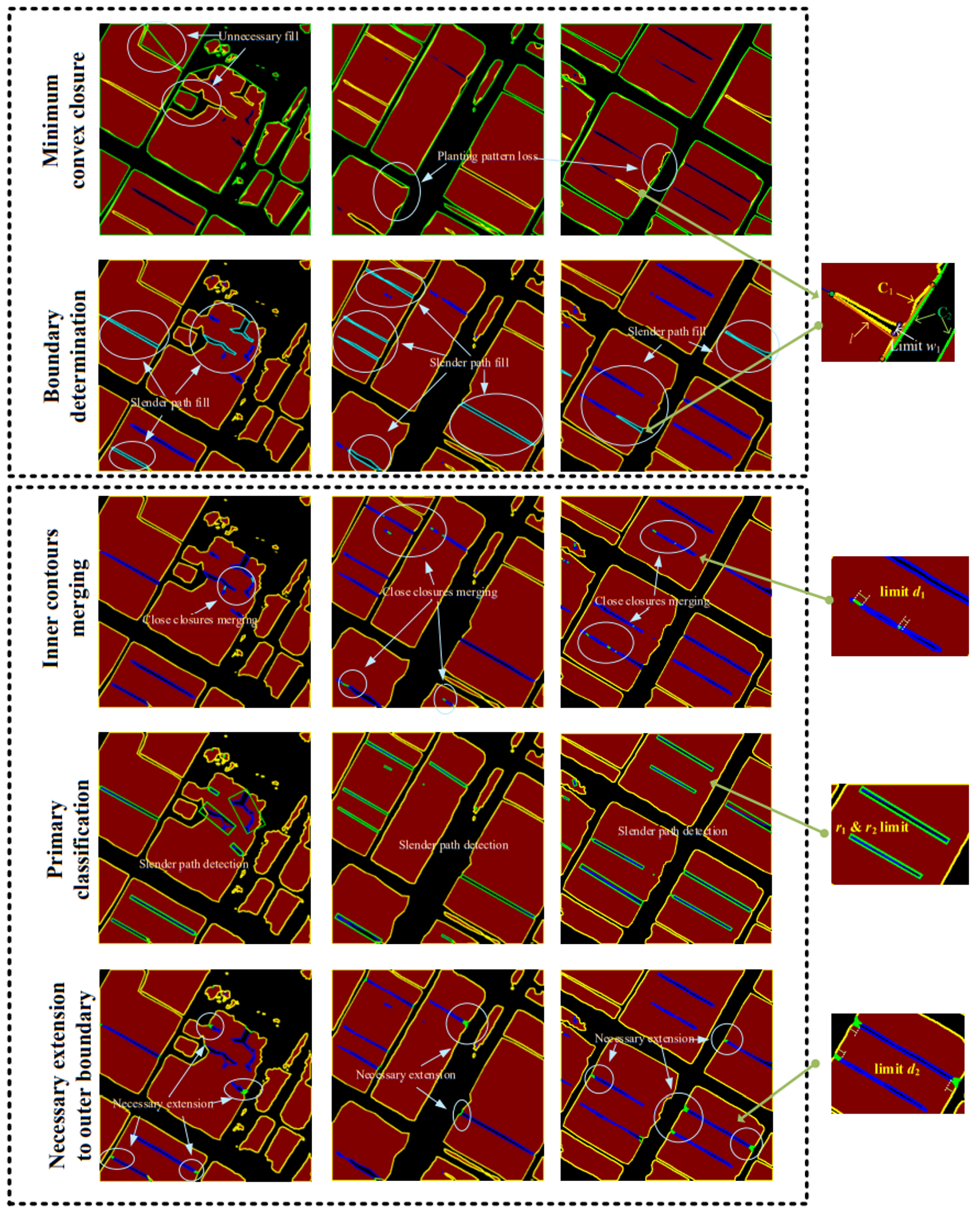
3.2. Delineation of Field Boundary and Inner Non-Planting Region

The aim of this section is to transfer the attained Semantic FPN-based map pixel classification results into fragmented contours. Attained contours should contain field boundaries and non-planting regions inside fields. These non-planting areas, including trees, water or waterway, slender walking paths, and electronic poles, would directly affect the calculation of crop planting statistics and make a great difference to the overall planning of agricultural machinery (plant protection and harvest).

To achieve raw contours based on semantic-output image pixels from the above-mentioned semantic FPN, we first employed a contour finding method proposed by Suzuki et al. [43]. The hierarchy between different attained contours was also achieved. We defined all attained raw contour collections as C, and the hierarchy information collection as H. As is seen in Figure 3, the slender non-planting area precision (such as a walking path or waterway) would make a great difference to the planting area boundary delineation. It may make the field boundary concave-shaped with deep steep corners. For field management or overall planning, the attained boundary was first improved using steep-corner removal, then followed by void-space analysis inside fields (non-planting area) as described in the following.

3.2.1. Boundary Delineation

This part was in order to shrink the effect of the slender path calculation error on the field boundary delineation. On the one hand, the calculation error could be caused by the satellite shooting angle; on the other, the slender characteristics (1~5 pixels in the raw map image) of the walking path or waterway could be greatly influenced by the learning quality of the convolutional network. We defined a steep-corner depth parameter as d (20~50 m), and a corner width limit parameter as w (2~5 m). The field boundary could be determined or improved based on the steps as following,

Step 1: Generate the minimum convex closure set as C₂ based on the raw outer contour set (defined as C₁) in C;

Step 2: Compare the closure point set between C₁ and C₂, find the point set erased from C₁ in C₂ defined as P, and the corresponding edge vertices in C₂ defined as E;

Step 3: Calculate the distance from each point P to its corresponding outer edge E, as L; for l_ij in L where i = 1, 2, …, I, j = 1, 2, …, J, I is the number of raw outer contour C₁ and J is the length of P;

Step 4: If max(l_i) < mean(l_i) + d, it means the erased points do not contain steep corners, and the field outer contour (i.e., boundary) should remain the same as that in C₁;

Step 5: If max(l_i) ≥ mean(l_i) + d, it means the erased points may contain a steep corner or steep corners; we then locate a point or some continuous points satisfying the condition max(l_i) ≥ mean(l_i) + d and their closest two points on each side as V. After this we calculate the distance between these two points in V as w₁; if w₁ ≤ w, it means a steep corner or steep corners does or do exist, in which case the field boundary should erase all points between the two points in V (not erasing V), while an inside contour between two points in V (containing V) should be generated as a point set along with hierarchy data.

These two defined parameters adopted in steps 4 and 5 were used to find deep slender corners inside fields and avoid identifying a deep concave area.

3.2.2. Non-Planting Area Detection

This section is to process the non-planting area (including necessary merging, primary classification, and extension) inside fields. The non-planting area could be a walking path, waterway, electric lines, transmission tower, trees, or a poor planting area. The non-planting area is crucial for overall planting management and planning (such as statistical analysis, and agricultural machinery path planning). We define s₁ and s₂ as inside-contour length-width ratio parameters and rectangle-area-contour area ratio parameters, respectively. This was done to determine whether the inside closure is slender or square-shaped, topologically. We also defined d₁ and d₂ as the merging limit parameter and extension limit parameter, respectively.

Step 1: Find the contours inside the same outer closure, and merge close contours based on the density-based spatial clustering of applications with noise [44] clustering. The minimum distance limit between vertices is set as d₁;

Step 2: Generate the bounding rectangle with a minimum area for each inner contour (updated after step 1), and calculate the length-width ratios as r₁ and rectangle area-contour area ratio as r₂ of each rectangle; the closure would be defined as a slender shape if r₁ < s₁ and r₁ < s₁, otherwise it would be defined as a square shape;

Step 3: For the closure marked with a slender shape, calculate the distance between each closure point and the outer boundary; the closure would be extended to the boundary if the calculated distance was less than d₂.

An example of the field boundary and agricultural pattern delineation process is shown in Figure 4.

3.3. Performance Evaluation

3.3.1. Semantic Segmentation Performance Metrics

To evaluate the image segmentation performance of the CNN model, we use four metrics, including the mean Intersection over Union (mIoU), Recall, Precision, and F1-score. Those metrics are described in the following equations,

$$\mathrm{mIoU}\left(Y,\stackrel{⌢}{Y}\right)=\frac{\left|Y\cap \stackrel{⌢}{Y}\right|}{\left|Y\cup \stackrel{⌢}{Y}\right|},$$

(2)

$$\mathrm{precision}=\frac{\mathrm{TP}}{\mathrm{TP}+\mathrm{FP}},$$

(3)

$$\mathrm{recall}=\frac{\mathrm{TP}}{\mathrm{TP}+\mathrm{FN}},$$

(4)

$$\mathrm{F}1=2\times \frac{\mathrm{precision}\times \mathrm{recall}}{\mathrm{precision}+\mathrm{recall}},$$

(5)

where TP, FP, TN, and FN denote the case numbers of true positives, false positives, true negatives, and false negatives, respectively. The greater values of those metrics (especially mIoU and F1) indicate better performance.

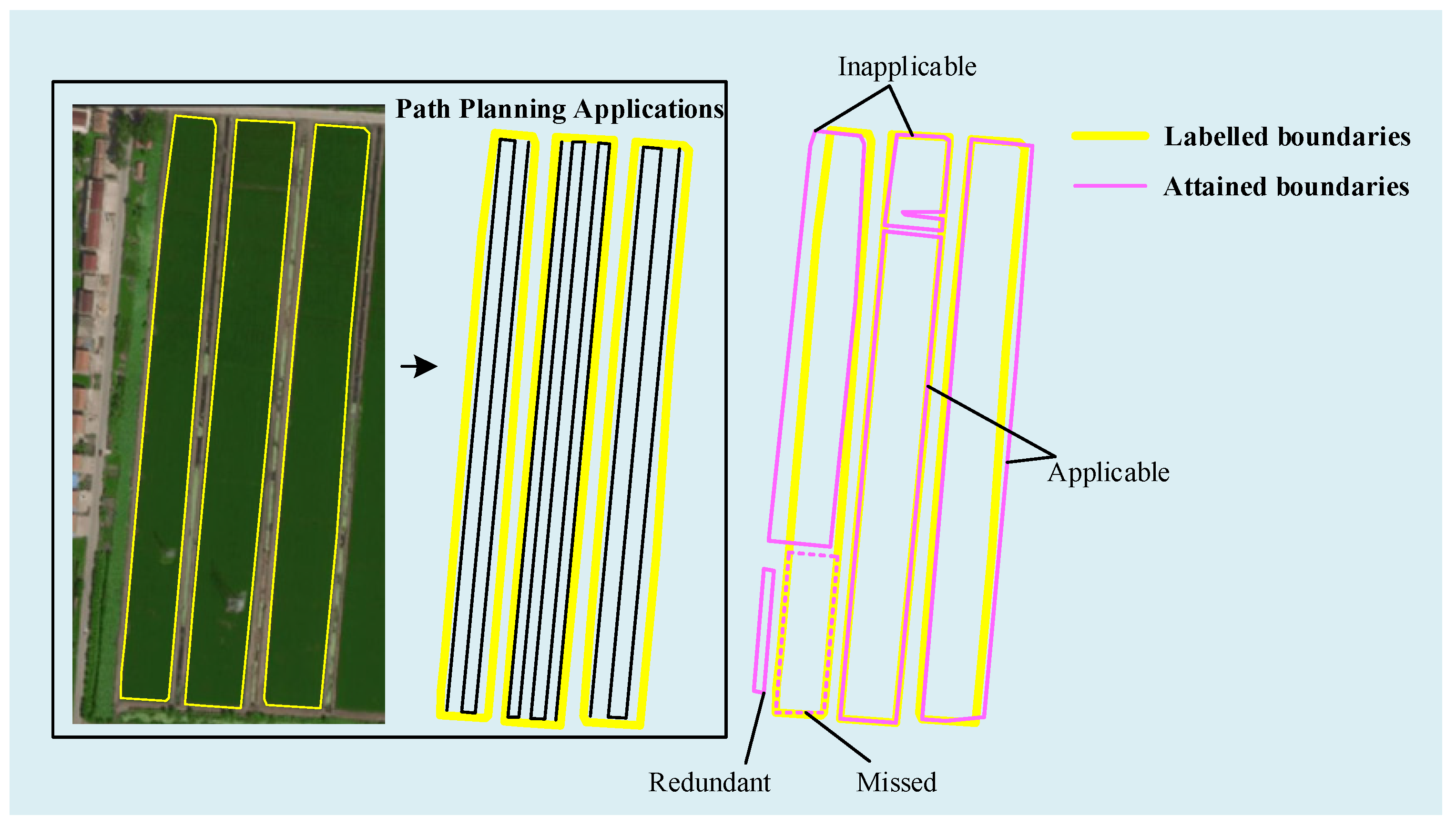
3.3.2. Attained Field Boundaries Evaluation

To validate the effective field boundaries using different methods, we defined four metrics, the applicable, inapplicable, redundant, and missed field boundaries for tractor path planning (see Figure 5). The defined applicable field boundary should contain over 90% intersection area of reference parcels, and have no unnecessary corners with 20 m depth from reference boundaries. Redundant field boundaries made up less than 10% intersection area of the reference parcels; the missed field boundaries referred to the un-detected parcel contours. The other attained boundaries were those inapplicable for machinery planning. It should be noted that the intact reference field boundary could be divided into several applicable closures, affected by the internal non-planting area (such as the un-annotated slender walking or waterway through the field).

4. Results

4.1. Experimental Set Up (Training Details)

The experiments were conducted by a workstation with an Intel i9-10980XE CPU, NVIDIA GeForce RTX 2080 GPU, and 64 GB of RAM memory. For convolution network training, our experiments were implemented in Keras with a Tensorflow backend; the early stop mechanism on the validation set was used to avoid over-fitting and evaluate the results; Adam was used as the optimizer, with a learning rate of 10⁻⁴. For contour determination and processing, the steep-corner depth parameter d was set to 10 (i.e., 5 m), the inside contour length-width ratio parameter s₁ and the rectangle area-contour area ratio parameter s₂ were set to 5 and 20, and the merging limit parameter and extension limit parameter were set to 30 and 20, respectively.

4.2. Proposed Method Performance Comparison

This section was to verify the field-planting-area semantic segmentation (pixel-wise classification) and boundary delineation, along with the internal non-planting region extraction performance of the proposed method.

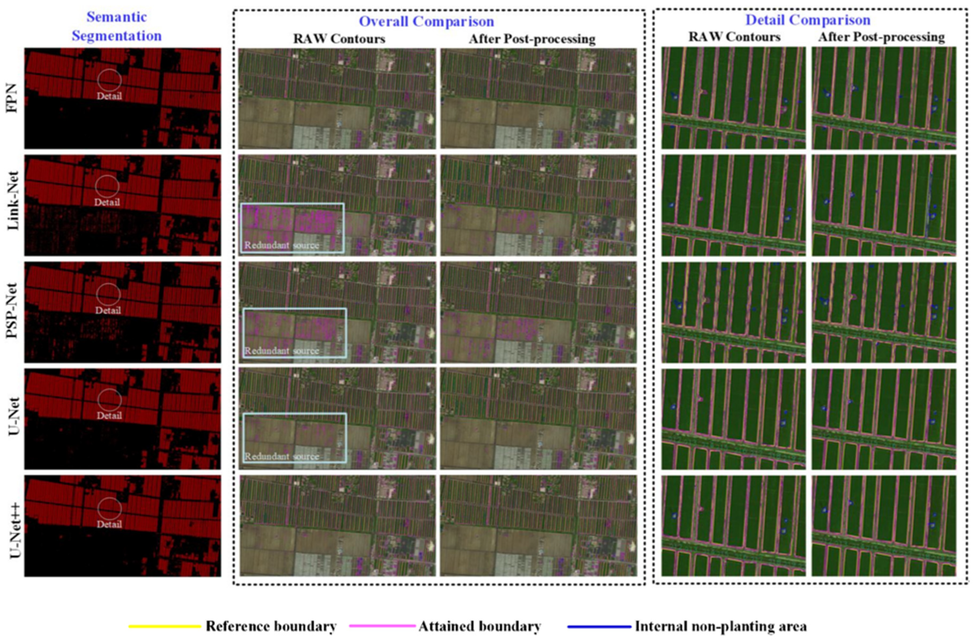
4.2.1. Pixel Classification Evaluation

We first evaluated the pixel classification metrics on extracting the planting region (i.e., field detection) using different convolutional networks, including FPN, Link-Net [45], PSP-Net [46], U-Net [47], and U-Net++ [48]. The evaluation metrics included the above-mentioned F1 score, IoU, Precision and Recall.

Table 1. Evaluation metric results using different semantic segmentation models without post-processing.

Method	IoU	F1 Score	Precision	Recall
FPN	0.8949	0.9339	0.9648	0.9274
Link-Net	0.9011	0.9419	0.9183	0.9813
PSP-Net	0.8637	0.9149	0.9543	0.9032
U-Net	0.9099	0.9472	0.9234	0.9852
U-Net++	0.9043	0.9433	0.9288	0.9735

reports the attained evaluation metric results using different convolutional network models, for agricultural area pixel classification.

As is seen in Table 1, the attained IoU value is around 0.90 and remains similar between different semantic segmentation models except in PSP-Net (0.86 merely). This means that some segmentation models can extract planting areas sufficiently. Similarly, the difference in the F1 score is quite minimal between the different neural networks except for PSP-Net, for which the attained score is around 0.94. However, the minimal difference in the attained F1 score does not mean that the attained precision and recall remained close to each other between different models. As is seen in Table 1, the value of precision using FPN and PSP-Net was greater than that when using Link-Net, U-Net, and U-Net++, while the attained recall based on FPN and PSP-Net remained much smaller than that when using the other models. There was a gap between the achieved precision and recall values for each model (around 0.05). This indicates that the values of FP and FN are greatly affected by the adopted neural networks referring to Equations (3) and (4). To investigate the effect of contour determination on pixel classification, we show in

Table 2. Evaluation metric results using different semantic segmentation models with post-processing on contours.

Method	IoU	F1 Score	Precision	Recall
FPN	0.8933	0.9329	0.9652	0.9255
Link-Net	0.8978	0.9399	0.9203	0.9757
PSP-Net	0.8621	0.9139	0.9549	0.9008
U-Net	0.9094	0.9470	0.9243	0.9837
U-Net++	0.9028	0.9423	0.9296	0.9711

the attained evaluation metric results based on different neural network models with the aforementioned contour post-processing.

The attained precision value in Table 2 increases compared with that in Table 1 when using the contour post-processing method. Similar to the results in Table 1, both the F1 score and IoU value attained the maximum when using U-Net++ and U-Net; the gap between recall and precision remained around 0.05 for each model even when using the contour post-processing method. However, all metrics in Table 2 changed but with a minimal leap, compared with those in Table 1. On the one hand, our post-processing work on contours was mainly concentrated on the slender path connection and extension. It would make a weak difference to the pixel-wise classification of planting and non-planting. On the other hand, all attained metric results were directly influenced by the dataset besides the convolutional network difference. Some non-planting areas, such as slender walking or water path, could have been easily marked as planting regions unintentionally.

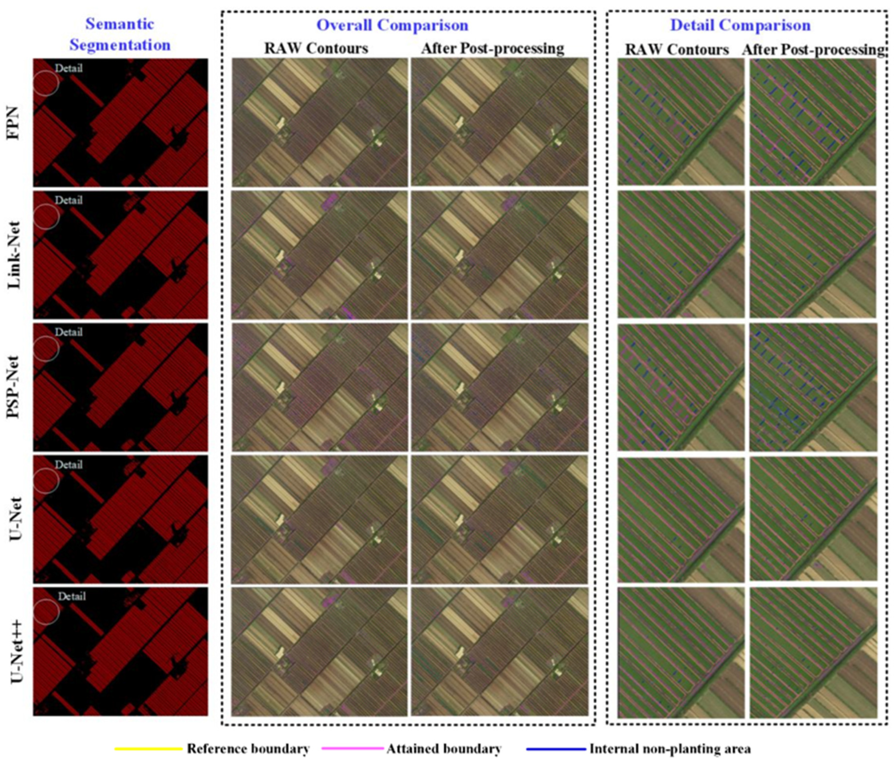
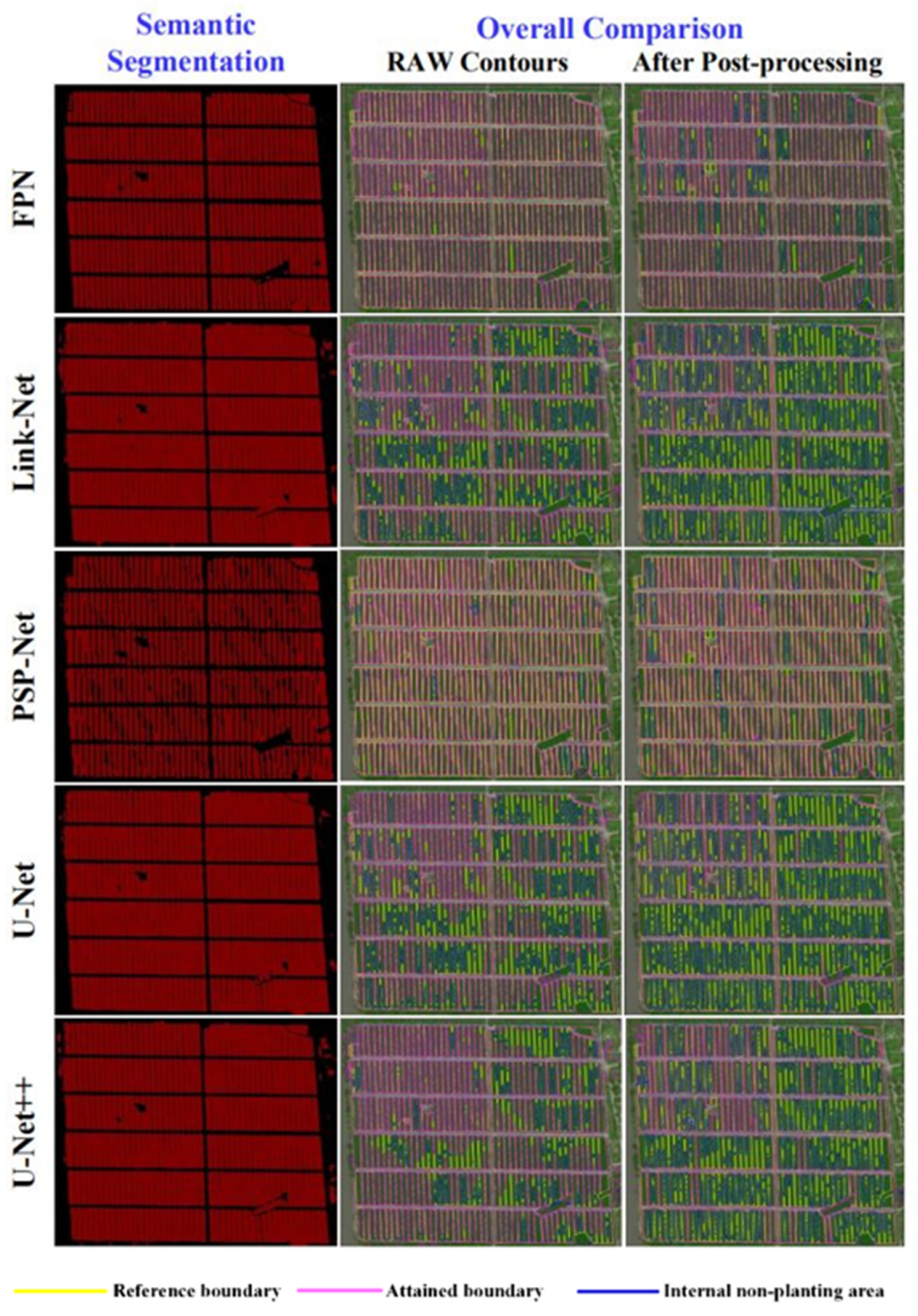
4.2.2. Attained Contour Verification on Different Sites

To evaluate the performance of the proposed contour post-processing method, we selected three study places (see Figure 6) with areas of 750 × 500 m, 770 × 500 m, and 300 × 500 m in sites 1, 2 and 3 from Figure 1, respectively. This is to facilitate the detailed visual analysis and discussion of different planting areas, considering the large area of each study site. Available reference field boundary data were also added, while the non-planting areas inside boundaries were not implemented.

Application in Study Site 1

It can be seen from Figure 7 that in study site 1, a larger scattered planting area (red spot on the left) was attained based on Link-Net, PSP-Net, U-Net, and U-Net++ than that using FPN, without the proposed post-processing method. This would greatly and directly expand the number of field boundaries, and agrees with the phenomenon of a lower value of precision using U-Net than those when using FPN and U-Net++ (high FP). Redundant field boundaries would be reduced after using the proposed post-processing method. The field boundary (line in magenta) and non-planting area (line in blue) inside the fields were attained using the post-processing method mentioned above. A few yellow-marked boundaries could be seen in the overall result using different methods with or without post-processing. In the detailed comparison section, a deep concave field boundary could be found without using the proposed methods, which could be improved after post-processing. Non-planting areas, especially telegraph poles, could be marked based on the post-processing method. It should be noted that the clouds and their shadows make a difference to the outer- and inner-contour extraction. The clouds can directly cover the planting area so that no compact boundary contour can be ascertained, with the field potentially split into two or three parts. To make a detailed comparison of the attained field boundary and non-planting zone contours, the obtained contour results are shown in

Table 3. Attained field boundaries number and planting status results in site 1.

Methods	Parcel Boundary Contour Number					Total Area/ha		Average Area/ha
	Applicable	Inapplicable	Redundant	Missed	Reference	Attained	Reference	Attained	Reference
FPN	276	60	293	0	317	447.83	440.02	0.71	1.39
Link-Net	237	35	7359	0		517.02		0.07
PSP-Net	316	21	872	0		462.30		0.38
U-Net	289	16	1118	0		495.95		0.35
U-Net++	264	32	1533	0		498.34		0.27
FPN ①	326	5	50	1		459.29		1.21
Link-Net ①	245	17	244	0		518.66		1.03
PSP-Net ①	297	5	251	1		471.68		0.85
U-Net ①	277	7	144	0		507.53		1.19
U-Net++ ①	264	22	142	0		508.18		1.19

Note: the superscript ① refers to the semantic segmentation model using the proposed post-processing method.

.

Table 3 shows that the number of applicable parcel boundary contours is close to the reference value when using PSP-Net and U-Net solely, and with FPN, PSP-Net, and X-Net after the proposed post-processing phase. The number of the missed parcel boundary contour is ≤1. In addition, both the inapplicable and redundant parcel boundary contour both shrank greatly when using the proposed post-processing method. This means the proposed post-processing procedure improves the quality of parcel boundary contour attainment, by eliminating redundant data. However, not all semantic algorithms can output high-quality boundary contours. The number of the achieved redundant contours was over 100 using Link-Net, PSP-Net, U-Net, and X-Net with proposed post-processing. It would take a great deal of effort to ease them for management and planning work. Moreover, the redundant contour would have a huge impact on the average field area determination. The total planted area value was close to the reference value when using FPN with or without post-processing. The value of the average area when using any semantic algorithm without post-processing was strictly less than 0.8 ha (0.07 ha using Link-Net), much lower than the reference value (1.34 ha). It was improved after post-processing to 1.20 ha.

Application in Study Site 2

Figure 8 shows that almost the whole field parcel was detected in the semantic results. While the non-planting areas had a huge impact on boundary contour results, redundant field contours were also high except when using FPN without post-processing. This is similar to the observation in Figure 7. It is worth noting that the attained field boundary (magenta line) agrees well with the reference boundary (yellow line). As shown in detail, the raw field boundary contour was greatly affected by the inside slender path and turned into a deep-concaved boundary. The slender path inside the field boundary is apparent in the detailed comparison, especially when using FPN and PSP-Net. By using the proposed post-processing method, the slender paths expanded and split the raw boundary contour into two or three sub-contours as applicable or inapplicable field boundaries. Obtained contour results from study site 2 are shown in

Table 4. Attained field boundary number and planting status results in site 2.

Methods	Parcel Boundary Contour Number					Total Area/ha		Average Area/ha
	Applicable	Inapplicable	Redundant	Missed	Reference	Attained	Reference	Attained	Reference
FPN	200	15	77	0	214	468.17	480.18	1.60	2.24
Link-Net	195	10	435	0		504.21		0.79
PSP-Net	195	25	104	0		460.22		1.42
U-Net	198	8	206	0		505.63		1.23
U-Net++	202	7	232	0		495.10		1.12
FPN ①	224	1	11	1		484.95		2.05
Link-Net ①	202	5	58	0		521.28		1.97
PSP-Net ①	215	2	32	1		481.22		1.93
U-Net ①	203	4	54	0		523.81		2.01
U-Net++ ①	206	3	51	0		512.98		1.97

Note: the superscript ① refers to the semantic segmentation models using the proposed post-processing method.

.

Similar to the results in Table 3, the applicable contour number expanded after post-processing; the number of attained applicable boundary contours was close to the reference values (214) when using FPN (224) or PSP-Net (215) post-processing. In addition, the post-processing procedure reduced the number of inapplicable and redundant contours at the same time. In a real-world application, this would save much energy for management and planning. However, the missed boundary number was strictly less than two using different models with or without the post-processing method, as shown in Table 4. The total planted area and average area both came close to the reference results when using FPN after post-processing (i.e., 484.95 ha → 480.18 ha for total area, 2.05 ha → 2.24 ha for the average area). It is worth noting that the redundant boundary contour greatly affected the average area calculation; the attained average area was 0.79 ha, which is much less than the reference value (2.24 ha).

Application in Study Site 3

As is seen in Figure 9, the reference boundary line (marked in yellow) was obvious when using Link-Net, U-Net, and U-Net++. As was more apparent in the semantic results, many field boundary contours were joined together except FPN and PSP-NET. This is due to the small-gap planting management mode, which caused blurred dividing lines between adjacent fields due to the remote sensing imagery. In addition, the non-planting contour (line in blue) number without processing exceeded that when using post-processing methods. This is because a large quantity of the raw boundary contours were deeply concaved. Compared with raw contours solely based on DNNs, attained contours, especially boundary delineation with post-processing, was much better using different models. Figure 8 shows that the number of field boundaries using FPN and PSP-Net was much lower than those when using other models, and the numbers of non-planting areas using Link-Net, U-Net, and U-Net++ were greatly elevated than when using FPN and PSP-Net.

Contrary to the results in the other study sites, the applicable parcel boundary number was quite different from the reference value, and reduced to less than 10 (272 as reference one), as shown in

Table 5. Attained field boundary number and planting status results in site 3.

Methods	Parcel Boundary Contour Number					Total Area/ha		Average Area/ha
	Applicable	Inapplicable	Redundant	Missed	Reference	Attained	Reference	Attained	Reference
FPN	221	17	8	1	272	27.44	29.94	0.11	0.11
Link-Net	18	23	36	0		34.22		0.44
PSP-Net	113	49	1	3		23.71		0.15
U-Net	23	31	0	5		33.76		0.63
U-Net++	2	14	26	1		35.82		0.85
FPN ①	220	3	0	5		30.53		0.14
Link-Net ①	27	2	3	1		37.03		1.16
PSP-Net ①	206	10	1	8		25.80		0.12
U-Net ①	28	3	1	1		36.34		1.14
U-Net++ ①	16	4	4	2		37.03		1.54

Note: the superscript ① refers to the semantic segmentation models using the proposed post-processing method.

. This aggerated the average planting area, which was obvious in Link-Net, U-Net, and U-Net++ especially after the post-processing phase. It was the small-scale and small-gap planting mode that made the greatest difference to this result. The applicable parcel boundary contour came close to the reference value only when using FPN with or without post-processing. Similar to in Table 4, the post-processing phase greatly reduced the number of inapplicable and redundant boundary contours. In addition, the total planting area came close to the reference value only when using FPN after post-processing. In addition, the average field area only reached that of the reference value when using FPN without post-processing, and PSP-Net after post-processing.

5. Conclusions

①

Semantic convolution neural network (CNN) models would have great effects on agricultural or planting parcel extraction; the attained IoU value (around 0.90) and F1 score (around 0.94) both remain close to each other when using FPN, Link-Net, U-Net, and U-Net++ with or without the proposed post-processing procedure, but the attained precision and recall is quite different using different models.

②

Agricultural field boundaries could be delineated in different study sites with varied planting modes (average area changes from 0.11 ha, 1.39 ha to 2.24 ha); in addition, internal non-planting areas, such as electronic poles, and walking or water paths, could greatly impact the field boundary result (especially slender path inside).

③

Applicable field boundary delineation is greatly affected by the semantic models and the post-processing method. A sharp decrease in inapplicable and redundant field boundaries took place in different study places after post-processing; in study site 1, inapplicable boundary number using FPN changed from 60 to 5, and redundant boundary number shrank from 7359 to 244 when using Link-Net; in study site 2, inapplicable boundary number using PSP-Net changed from 25 to 2, and the redundant boundary number shrank from 435 to 58 when using Link-Net; and in study site 3, inapplicable boundary number using PSP-Net changed from 49 to 10, and redundant boundary number shrank from 36 to 3 when using Link-Net.

④

The determined applicable boundary number, total, and average planting area generally remain closer to the reference values when using the proposed methodology (i.e., semantic FPN with post-processing) in the three different study sites, compared with other methods. Moreover, the number of inapplicable, redundant, and missed field boundaries also remain the lowest, which helps to avoid the unnecessary wasting of management and planning time on machinery operations.

⑤

Besides the extraction models, the planting mode also greatly affects the boundary extraction; small-scale and small-gap planting would weaken the field boundary delineation performance.

References

1. Bogunovic, I.; Pereira, P.; Brevik, E.C. Spatial distribution of soil chemical properties in an organic farm in Croatia. Sci. Total Environ. 2017, 584, 535–545. [Google Scholar] [CrossRef] [PubMed] [Green Version]
2. Tetteh, G.O.; Gocht, A.; Conrad, C. Optimal parameters for delineating agricultural parcels from satellite images based on supervised Bayesian optimization. Comput. Electron. Agric. 2020, 178, 105696. [Google Scholar] [CrossRef]
3. Lobert, F.; Holtgrave, A.K.; Schwieder, M.; Pause, M.; Vogt, J.; Gocht, A.; Erasmi, S. Mowing event detection in permanent grasslands: Systematic evaluation of input features from Sentinel-1, Sentinel-2, and Landsat 8 time series. Remote Sens. Environ. 2021, 267, 112751. [Google Scholar] [CrossRef]
4. Kanjir, U.; Đurić, N.; Veljanovski, T. Sentinel-2 based temporal detection of agricultural land use anomalies in support of common agricultural policy monitoring. ISPRS Int. J. Geo-Inf. 2018, 7, 405. [Google Scholar] [CrossRef] [Green Version]
5. Atzberger, C. Advances in remote sensing of agriculture: Context description, existing operational monitoring systems and major information needs. Remote Sens. 2013, 5, 949–981. [Google Scholar] [CrossRef] [Green Version]
6. Rahman, M.; Ishii, K.; Noguchi, N. Optimum harvesting area of convex and concave polygon field for path planning of robot combine harvester. Intell. Serv. Robot. 2019, 12, 167–179. [Google Scholar] [CrossRef] [Green Version]
7. Dorigo, W.A.; Zurita-Milla, R.; de Wit, A.J.W.; Brazile, J.; Singh, R.; Schaepman, M.E. A review on reflective remote sensing and data assimilation techniques for enhanced agroecosystem modeling. Int. J. Appl. Earth Obs. Geoinf. 2007, 9, 165–193. [Google Scholar] [CrossRef]
8. Bellón, B.; Bégué, A.; Lo Seen, D.; De Almeida, C.A.; Simões, M. A remote sensing approach for regional-scale mapping of agricultural land-use systems based on NDVI time series. Remote Sens. 2017, 9, 600. [Google Scholar] [CrossRef] [Green Version]
9. Smith, W.K.; Dannenberg, M.P.; Yan, D.; Herrmann, S.; Barnes, M.L.; Barron-Gafford, G.A.; Biederman, J.A.; Ferrenberg, S.; Fox, A.M.; Hudson, A.; et al. Remote sensing of dryland ecosystem structure and function: Progress, challenges, and opportunities. Remote Sens. Environ. 2019, 233, 111401. [Google Scholar] [CrossRef]
10. Liu, X.; Zhai, H.; Shen, Y.; Lou, B.; Jiang, C.; Li, T.; Husain, S.B.; Shen, G. Large-scale crop mapping from multisource remote sensing images in google earth engine. IEEE J. Sel. Top. Appl. Earth Obs. Remote Sens. 2020, 13, 414–427. [Google Scholar] [CrossRef]
11. Paudel, D.; Boogaard, H.; de Wit, A.; Janssen, S.; Osinga, S.; Pylianidis, C.; Athanasiadis, I.N. Machine learning for large-scale crop yield forecasting. Agric. Syst. 2021, 187, 103016. [Google Scholar] [CrossRef]
12. Ji, Z.; Pan, Y.; Zhu, X.; Wang, J.; Li, Q. Prediction of crop yield using phenological information extracted from remote sensing vegetation index. Sensors 2021, 21, 1406. [Google Scholar] [CrossRef] [PubMed]
13. Waldner, F.; Lambert, M.J.; Li, W.; Weiss, M.; Demarez, V.; Morin, D.; Marais-Sicre, C.; Hagolle, O.; Baret, F.; Defourny, P. Land cover and crop type classification along the season based on biophysical variables retrieved from multi-sensor high-resolution time series. Remote Sens. 2015, 7, 10400–10424. [Google Scholar] [CrossRef] [Green Version]
14. Kussul, N.; Lavreniuk, M.; Skakun, S.; Shelestov, A. Deep learning classification of land cover and crop types using remote sensing data. IEEE Geosci. Remote Sens. Lett. 2017, 14, 778–782. [Google Scholar] [CrossRef]
15. Orynbaikyzy, A.; Gessner, U.; Conrad, C. Crop type classification using a combination of optical and radar remote sensing data: A review. Int. J. Remote Sens. 2019, 40, 6553–6595. [Google Scholar] [CrossRef]
16. Xu, D.; Guo, X. Some insights on grassland health assessment based on remote sensing. Sensors 2015, 15, 3070–3089. [Google Scholar] [CrossRef] [Green Version]
17. Gogoi, N.K.; Deka, B.; Bora, L.C. Remote sensing and its use in detection and monitoring plant diseases: A review. Agric. Rev. 2018, 39. [Google Scholar] [CrossRef]
18. Ennouri, K.; Triki, M.A.; Kallel, A. Applications of remote sensing in pest monitoring and crop management. In Bioeconomy for Sustainable Development; Springer: Singapore, 2020; pp. 65–77. [Google Scholar] [CrossRef]
19. Sa, I.; Popović, M.; Khanna, R.; Chen, Z.; Lottes, P.; Liebisch, F.; Nieto, J.; Stachniss, C.; Walter, A.; Siegwart, R. WeedMap: A large-scale semantic weed mapping framework using aerial multispectral imaging and deep neural network for precision farming. Remote Sens. 2018, 10, 1423. [Google Scholar] [CrossRef] [Green Version]
20. Dalezios, N.R.; Dercas, N.; Spyropoulos, N.V.; Psomiadis, E. Remotely Sensed Methodologies for Crop Water Availability and Requirements in Precision Farming of Vulnerable Agriculture. Water Resour. Manag. 2019, 33, 1499–1519. [Google Scholar] [CrossRef]
21. Persello, C.; Tolpekin, V.A.; Bergado, J.R.; de By, R.A. Delineation of agricultural fields in smallholder farms from satellite images using fully convolutional networks and combinatorial grouping. Remote Sens. Environ. 2019, 231, 111253. [Google Scholar] [CrossRef]
22. Kumar, M.S.; Jayagopal, P. Delineation of field boundary from multispectral satellite images through U-Net segmentation and template matching. Ecol. Inform. 2021, 64, 101370. [Google Scholar] [CrossRef]
23. Zhang, H.; Liu, M.; Wang, Y.; Shang, J.; Liu, X.; Li, B.; Song, A.; Li, Q. Automated delineation of agricultural field boundaries from Sentinel-2 images using recurrent residual U-Net. Int. J. Appl. Earth Obs. Geoinf. 2021, 105, 102557. [Google Scholar] [CrossRef]
24. Waldner, F.; Diakogiannis, F.I.; Batchelor, K.; Ciccotosto-Camp, M.; Cooper-Williams, E.; Herrmann, C.; Mata, G.; Toovey, A. Detect, consolidate, delineate: Scalable mapping of field boundaries using satellite images. Remote Sens. 2021, 13, 2197. [Google Scholar] [CrossRef]
25. Turker, M.; Kok, E.M. Field-based sub-boundary extraction from remote sensing imagery using perceptual grouping. ISPRS J. Photogramm. Remote Sens. 2013, 79, 106–121. [Google Scholar] [CrossRef]
26. Yan, L.; Roy, D.P. Automated crop field extraction from multi-temporal web enabled Landsat data. Remote Sens. Environ. 2014, 144, 42–64. [Google Scholar] [CrossRef] [Green Version]
27. Graesser, J.; Ramankutty, N. Detection of cropland field parcels from Landsat imagery. Remote Sens. Environ. 2017, 201, 165–180. [Google Scholar] [CrossRef] [Green Version]
28. Segl, K.; Kaufmann, H. Detection of small objects from high-resolution panchromatic satellite imagery based on supervised image segmentation. IEEE Trans. Geosci. Remote Sens. 2001, 39, 2080–2083. [Google Scholar] [CrossRef]
29. Da Costa, J.P.; Michelet, F.; Germain, C.; Lavialle, O.; Grimier, G. Delineation of vine parcels by segmentation of high resolution remote sensed images. Precis. Agric. 2007, 8, 95–110. [Google Scholar] [CrossRef]
30. García-Pedrero, A.; Gonzalo-Martín, C.; Lillo-Saavedra, M. A machine learning approach for agricultural parcel delineation through agglomerative segmentation. Int. J. Remote Sens. 2017, 38, 1809–1819. [Google Scholar] [CrossRef] [Green Version]
31. Wang, L.; Zhao, Y.; Liu, S.; Li, Y.; Chen, S.; Lan, Y. Precision detection of dense plums in orchards using the improved YOLOv4 model. Front. Plant Sci. 2022, 13, 839269. [Google Scholar] [CrossRef]
32. Wagner, M.P.; Oppelt, N. Extracting Agricultural Fields from Remote Sensing Imagery Using Graph-Based Growing Contours. Remote Sens. 2020, 12, 1205. [Google Scholar] [CrossRef] [Green Version]
33. Hong, R.; Park, J.; Jang, S.; Shin, H.; Kim, H.; Song, I. Development of a parcel-level land boundary extraction algorithm for aerial imagery of regularly arranged agricultural areas. Remote Sens. 2021, 13, 1167. [Google Scholar] [CrossRef]
34. North, H.C.; Pairman, D.; Belliss, S.E. Boundary Delineation of Agricultural Fields in Multitemporal Satellite Imagery. IEEE J. Sel. Top. Appl. Earth Obs. Remote Sens. 2019, 12, 237–251. [Google Scholar] [CrossRef]
35. Taravat, A.; Wagner, M.P.; Bonifacio, R.; Petit, D. Advanced fully convolutional networks for agricultural field boundary detection. Remote Sens. 2021, 13, 722. [Google Scholar] [CrossRef]
36. Xu, L.; Ming, D.; Du, T.; Chen, Y.; Dong, D.; Zhou, C. Delineation of cultivated land parcels based on deep convolutional networks and geographical thematic scene division of remotely sensed images. Comput. Electron. Agric. 2022, 192, 106611. [Google Scholar] [CrossRef]
37. Lv, Y.; Zhang, C.; Yun, W.; Gao, L.; Wang, H.; Ma, J.; Li, H.; Zhu, D. The delineation and grading of actual crop production units in modern smallholder areas using RS Data and Mask R-CNN. Remote Sens. 2020, 12, 1074. [Google Scholar] [CrossRef]
38. Chiu, M.T.; Xu, X.; Wei, Y.; Huang, Z.; Schwing, A.; Brunner, R.; Khachatrian, H.; Karapetyan, H.; Dozier, I.; Rose, G.; et al. Agriculture-vision: A large aerial image database for agricultural pattern analysis. In Proceedings of the IEEE Computer Society Conference on Computer Vision and Pattern Recognition, Seattle, WA, USA, 13–19 June 2020; pp. 2825–2835. [Google Scholar] [CrossRef]
39. Oksanen, T.; Visala, A. Coverage path planning algorithms for agricultural field machines. J. Field Robot. 2009, 8, 651–668. [Google Scholar] [CrossRef]
40. Cabreira, T.; Brisolara, L.; Ferreira, P. Survey on Coverage Path Planning with Unmanned Aerial Vehicles. Drones 2019, 3, 4. [Google Scholar] [CrossRef] [Green Version]
41. Xu, Y.; Sun, Z.; Xue, X.; Gu, W.; Peng, B. A hybrid algorithm based on MOSFLA and GA for multi-UAVs plant protection task assignment and sequencing optimization. Appl. Soft Comput. J. 2020, 96, 106623. [Google Scholar] [CrossRef]
42. Kirillov, A.; Girshick, R.; He, K.; Dollar, P. Panoptic feature pyramid networks. In Proceedings of the IEEE Computer Society Conference on Computer Vision and Pattern Recognition, Long Beach, CA, USA, 15–20 June 2019; pp. 6392–6401. [Google Scholar] [CrossRef] [Green Version]
43. Suzuki, S.; Be, K. Topological structural analysis of digitized binary images by border following. Comput. Vis. Graph. Image Process. 1985, 30, 32–46. [Google Scholar] [CrossRef]
44. Chen, Y.; Zhou, L.; Pei, S.; Yu, Z.; Chen, Y.; Liu, X.; Du, J.; Xiong, N. Knn-Block Dbscan: Fast Clustering for Large-Scale Data. IEEE Trans. Syst. Man Cybern. Syst. 2021, 51, 3939–3953. [Google Scholar] [CrossRef]
45. Chaurasia, A.; Culurciello, E. LinkNet: Exploiting encoder representations for efficient semantic segmentation. In Proceedings of the 2017 IEEE Visual Communications and Image Processing (VCIP 2017), St. Petersburg, FL, USA, 10–13 December 2017; pp. 1–4. [Google Scholar] [CrossRef] [Green Version]
46. Zhao, H.; Shi, J.; Qi, X.; Wang, X.; Jia, J. Pyramid scene parsing network. In Proceedings of the 2017 IEEE Conference on Computer Vision and Pattern Recognition (CVPR 2017), Honolulu, HI, USA, 21–26 July 2017; pp. 6230–6239. [Google Scholar] [CrossRef] [Green Version]
47. Ronneberger, O.; Fischer, P.; Brox, T. U-net: Convolutional networks for biomedical image segmentation. In Proceedings of the International Conference on Medical Image Computing and Computer-Assisted Intervention, Munich, Germany, 5–7 October 2015; Springer: Cham, Switzerland, 2015; pp. 234–241. [Google Scholar] [CrossRef] [Green Version]
48. Zhou, Z.; Rahman Siddiquee, M.M.; Tajbakhsh, N.; Liang, J. Unet++: A nested u-net architecture for medical image segmentation. In Deep Learning in Medical Image Analysis and Multimodal Learning for Clinical Decision Support; Springer: Cham, Switzerland, 2018; pp. 3–11. [Google Scholar] [CrossRef] [Green Version]
Figure 1. Location and satellite map imagery of the selected study and verification sites.
Remotesensing 15 02937 g001
Figure 2. The structure of the adopted semantic FPN model.
Remotesensing 15 02937 g002
Figure 3. Raw closures attained based on semantic FPN and contour-finding method.
Remotesensing 15 02937 g003
Figure 4. An example of field boundary and agricultural pattern delineation.
Remotesensing 15 02937 g004
Figure 5. Example of attained contours applicable, inapplicable, redundant and missed for the path-planning of crop-protection UAV or Harvest Tractors.
Remotesensing 15 02937 g005
Figure 6. Selected study place and reference boundary contours in three different sites.
Remotesensing 15 02937 g006
Figure 7. Attained agricultural parcels, boundaries and internal non-planting areas in site 1.
Remotesensing 15 02937 g007
Figure 8. Attained agricultural parcels, boundaries and internal non-planting areas in site 2.
Remotesensing 15 02937 g008
Figure 9. Attained agricultural parcels, boundaries and internal non-planting areas in site 3.
Remotesensing 15 02937 g009