Article

MCPT: Mixed Convolutional Parallel Transformer for Polarimetric SAR Image Classification

1
School of Computer Science and Technology, Henan Polytechnic University, Jiaozuo 454003, China
2
School of Computer and Information Engineering, Henan Normal University, Xinxiang 453007, China
*
Author to whom correspondence should be addressed.
Remote Sens. 2023, 15(11), 2936; https://doi.org/10.3390/rs15112936
Submission received: 5 May 2023 / Revised: 31 May 2023 / Accepted: 2 June 2023 / Published: 5 June 2023

Abstract

:
Vision transformers (ViT) have the characteristics of massive training data and complex model, which cannot be directly applied to polarimetric synthetic aperture radar (PolSAR) image classification tasks. Therefore, a mixed convolutional parallel transformer (MCPT) model based on ViT is proposed for fast PolSAR image classification. First of all, a mixed depthwise convolution tokenization is introduced. It replaces the learnable linear projection in the original ViT to obtain patch embeddings. The process of tokenization can reduce computational and parameter complexity and extract features of different receptive fields as input to the encoder. Furthermore, combining the idea of shallow networks with lower latency and easier optimization, a parallel encoder is implemented by pairing the same modules and recombining to form parallel blocks, which can decrease the network depth and computing power requirement. In addition, the original class embedding and position embedding are removed during tokenization, and a global average pooling layer is added after the encoder for category feature extraction. Finally, the experimental results on AIRSAR Flevoland and RADARSAT-2 San Francisco datasets show that the proposed method achieves a significant improvement in training and prediction speed. Meanwhile, the overall accuracy achieved was 97.9% and 96.77%, respectively.

Graphical Abstract

1. Introduction

Synthetic Aperture Radar (SAR) [1] is a remote sensing sensor belonging to the active imaging technology that operates in the microwave band. It has many extraordinary characteristics, such as full-time work, being less affected by weather and certain penetration ability to ground objects [2,3,4,5]. Therefore, SAR-related applications affect various aspects of human production and life, such as land use, urban planning and crop yield assessment [6]. Polarimetric SAR (PolSAR) is a type of SAR that works in different forms of polarization combinations. It captures information on object material composition, geometric features and azimuth, and provides more comprehensive object descriptions for different deployment scenarios. Thus, it has become a research hotspot in the field of SAR remote sensing [7]. PolSAR image classification [8] refers to the process of dividing all pixels in an image into a specific category according to specific rules. It is a fundamental research direction in PolSAR image understanding and interpretation techniques. Automatically analyzing radar image features to classify and recognize images is very beneficial in improving the efficiency of human image understanding, while also greatly enhancing the ability of people to obtain image information.
In traditional PolSAR image feature extraction methods, such as polarization target decomposition [9], the scattering mechanisms of targets are interpreted based on practical physical constraints. The polarimetric data are decomposed into several physically meaningful parameters to facilitate the analysis of complex scattering processes. So far, several decomposition methods have been proposed, including Cameron decomposition [10], Cloude–Pottier decomposition [11,12], Krogager decomposition [13], and so on. However, these methods can only determine target scattering types and not specifically classify them into land cover types. Moreover, large amounts of PolSAR data are being obtained with the maturing development of various earth observation platforms. Traditional methods based on polarization decomposition and data characteristics cannot meet the expanding interpretation requirements. At the same time, deep learning technology has continued to evolve, demonstrating powerful capabilities for processing data and extracting features. As a result, more and more researchers are applying it to PolSAR image classification research [14]. Compared to traditional methods, deep learning methods use labeled data to train neural networks to obtain features, establish relationships between data feature information and categories, and predict the category of unknown pixels. Such data-driven feature extraction frameworks are also known as representation learning [15].
At present, convolutional neural networks (CNNs) [16] are the most widely used representation learning method in PolSAR image classification tasks. Zhou et al. [17] first studied the application of deep CNNs in PolSAR image classification and designed a four-layer CNN customized for PolSAR image classification that automatically learns different levels of polarized spatial features from data through two cascaded convolutional layers. By taking the spatial characteristics of PolSAR images into account, it is able to successfully distinguish between sloping built-up areas with vegetation. These are often mixed in the polarization feature space. Since then, various CNN variants for PolSAR image classification have been proposed. For example, Chen et al. [18] attempted to exploit a limited number of labeled samples to train deep CNNs for PolSAR image classification and proposed a polarimetric-feature-driven deep CNN classification scheme. Classic roll invariant polarimetric features and hidden polarimetric features in the rotation domain were used to support the training of the deep CNN classifier and to enhance the final classification performance. The model has better performance compared with traditional CNN. However, the polarization features used for training are derived from field knowledge [19,20,21], which makes the acquisition of labeled data for the method a time-consuming and difficult task. Yang et al. [22] pointed out that selecting an appropriate number of high-quality features obtained by target decomposition of PolSAR images is crucial for the tasks. Thus, a CNN-based PolSAR image classification feature selection method was proposed to select feature subsets. The best-performing one is selected as the final result. Taking the performance of feature combinations into account, the selected subset of features performs better in both traditional and deep learning classification methods. In order to improve the performance of CNNs on limited training data, Shang et al. [23] proposed a new densely connected and depthwise separable convolutional neural network. Depthwise separable convolution extracts features independently from each channel of the PolSAR image and dense connection is introduced to directly connect non-adjacent layers. In this way, it can avoid extracting redundant features, reuse different levels of feature maps from PolSAR images and reduce the number of training parameters. Nonetheless, as research on CNN-based PolSAR image classification continues to deepen, the locality caused by inductive biases has become a bottleneck restricting its performance, making it difficult for CNN-based PolSAR image classification methods to make further improvements.
The transformer [24] model was originally proposed in the field of natural language processing (NLP), mainly by pre-training on a large text corpus, followed by fine-tuning on a smaller specific task dataset. Inspired by the success of the transformer in NLP, Dosovitskiy et al. [25] proposed a vision transformer model that can be easily applied to the image domain with minimal modifications to the standard transformer model. ViT utilizes a self-attention mechanism (SA) [24] to replace tokens (words) in languages with image patches, which can achieve remote interaction between pixels and capture global correlations in the image domain [26]. Dong et al. [27] explored the ViT model for PolSAR image classification in detail and proposed a representation learning framework based on ViT, which included both supervised and unsupervised learning. In the supervised learning framework, image patches are used as input, and SA is utilized to extract global features. In addition, an improved contrastive-based strategy is introduced to achieve simple unsupervised representation learning. Compared to CNNs and their variants, ViT improves classification performance by building more global representations, while also demonstrating robustness to the initial input form. These studies may prompt people to rethink the dominant position of CNNs in PolSAR image classification. As research on ViT in PolSAR image classification continues to deepen, many ViT-based classification methods have emerged. For example, Wang et al. [28] pointed out that the scarcity of PolSAR-labeled samples and the small receptive field of models limit the performance of deep learning methods for PolSAR image classification and then proposed a ViT-based classification method. It can receive PolSAR images of different resolutions and is pre-trained with masked autoencoders with unlabeled data to address the problem of scarce labeled data. Correspondingly, Jamali et al. [29] demonstrated that the main problem with applying ViT to PolSAR image classification is the scarcity of labeled data and proposed a ViT-based framework. Both 3-D and 2-D CNNs are adopted as feature extractors and a local window attention is implemented to enhance local feature representation power for effective classification of PolSAR data. Therefore, it can greatly reduce annotation costs and hardware requirements.
As can be seen from the existing work, most of the ViT-based classification methods proposed so far are basic applications of ViT to PolSAR image classification tasks. There is a lack of deeper integration and exploration between ViT and PolSAR image classification. However, convolutional structures still dominate in PolSAR image representation learning and classification. The local nature of convolution is not always advantageous as it extracts local neighborhood features and does not take the global information into account. Consequently, when extracting features from PolSAR patches centered around the input pixels, there is a large amount of local information in the extracted features that leads to low efficiency or accuracy. Although the application of ViT partially addresses these issues, research on ViT in PolSAR image classification is still limited and not deep enough. In addition, the pre-training of ViT requires sufficient labeled data but annotating every pixel in a PolSAR dataset is time-consuming and costly. Based on the above analysis and inspired by previous works, a mixed convolutional parallel transformer model is proposed for PolSAR image classification. It improves the original ViT model with better targeting for PolSAR image classification. Furthermore, the model achieves higher training and prediction speed while maintaining high accuracy with fewer parameters and lower computational cost. There are three main improvements to the proposed model:
(1)
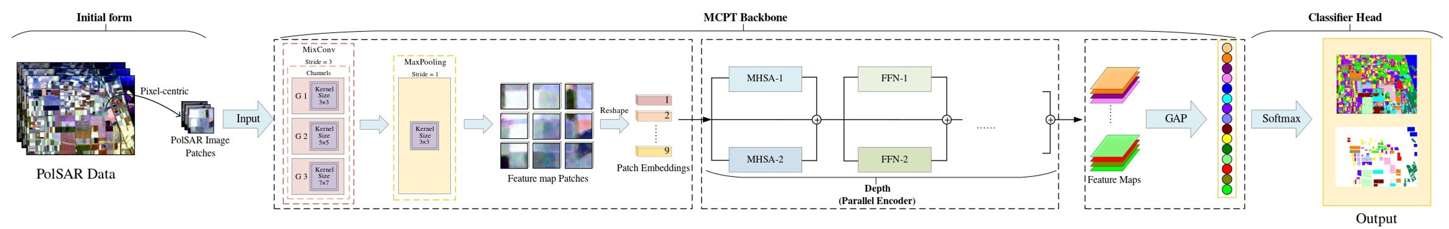
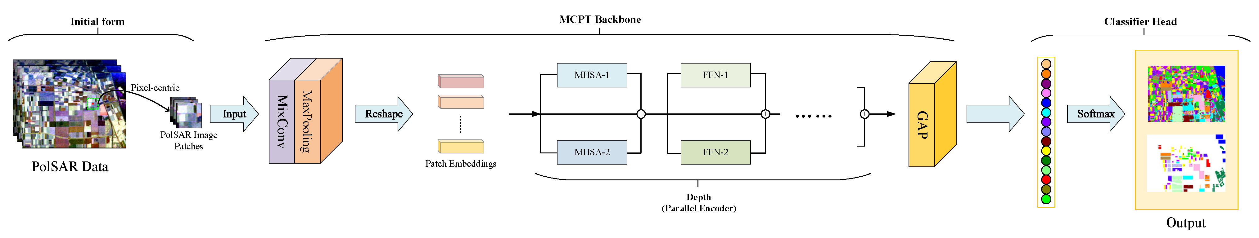
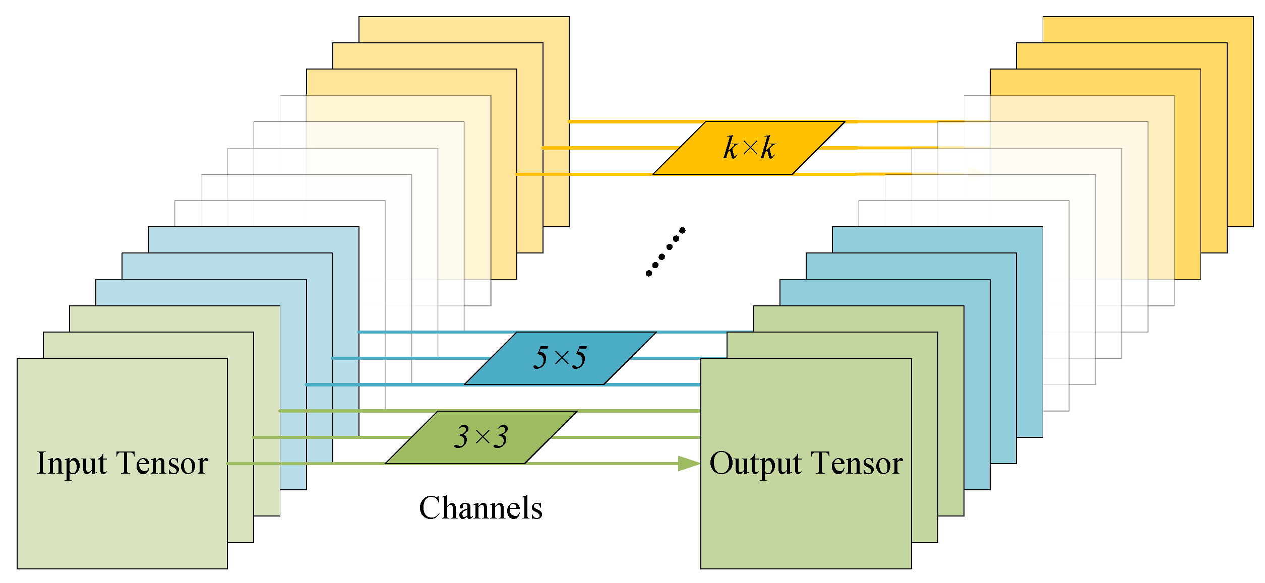
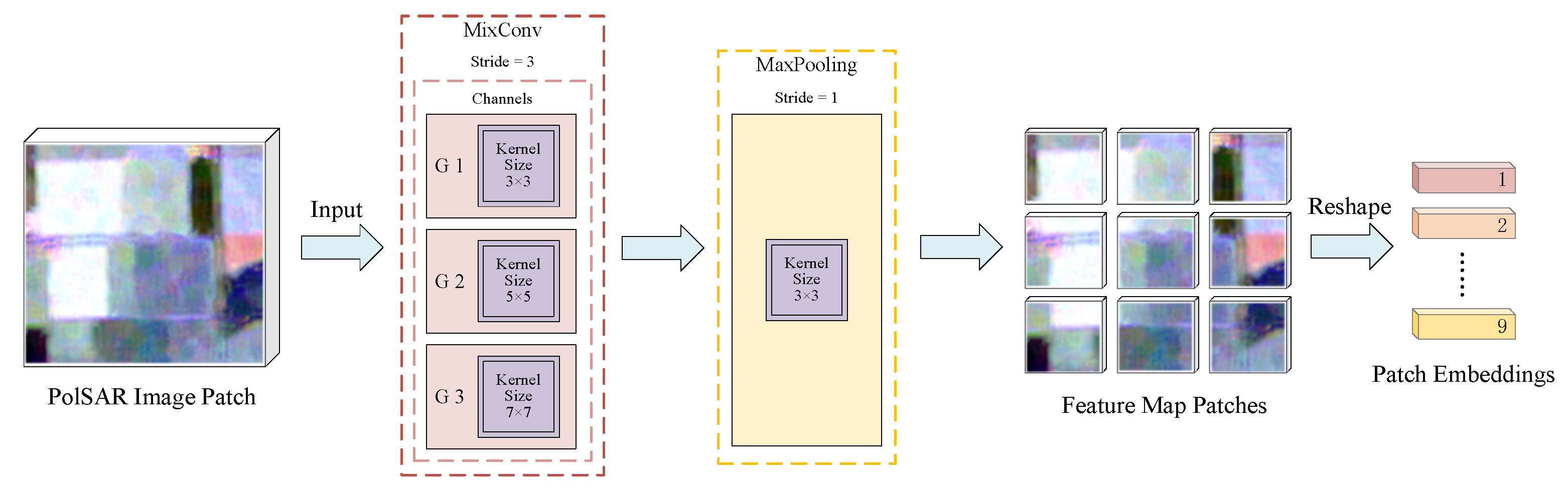
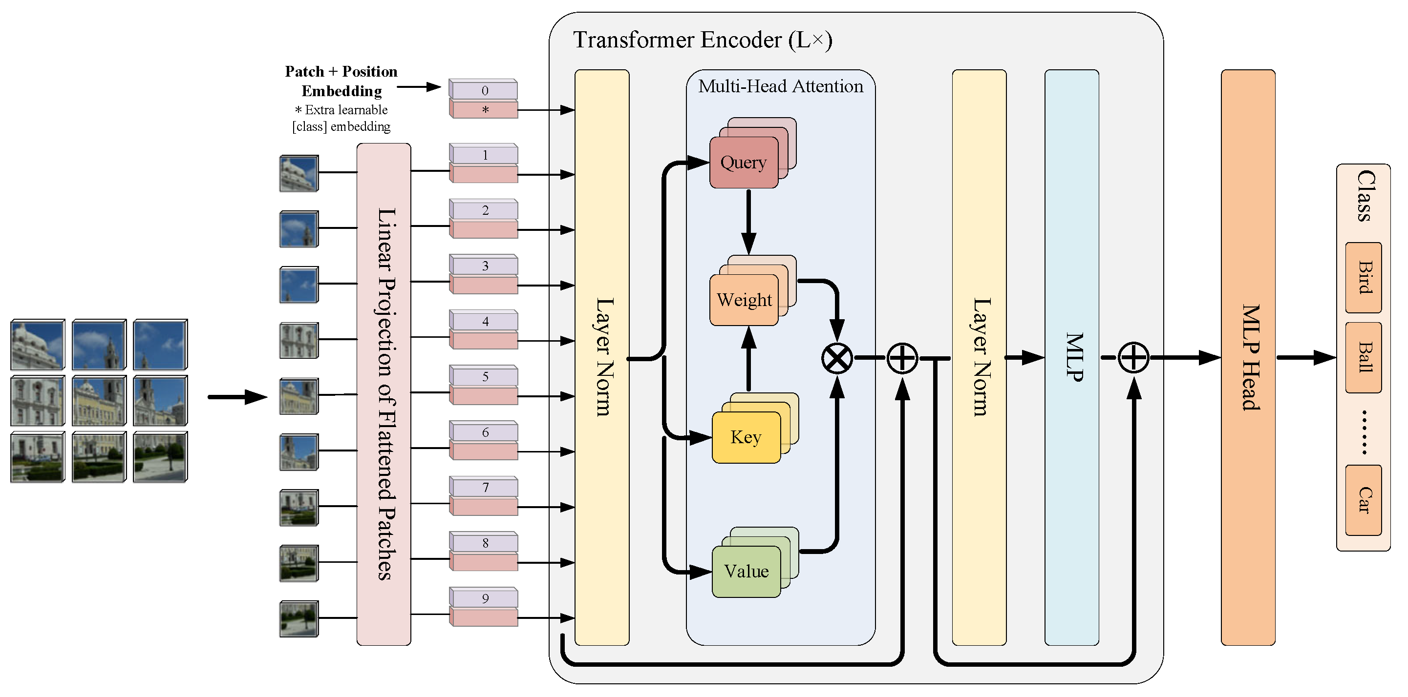
Mixed depthwise convolution tokenization. A mixed depthwise convolution (MixConv) is introduced in the data pre-processing part of the model for the tokenization of the input data, which replaces the linear projection used in the original ViT. MixConv naturally mixes multiple kernel sizes in a single convolution and can extract feature maps with different receptive fields at the same time. This tokenization process makes the proposed method more flexible than the original ViT. It is no longer limited by the input resolution, which must be strictly divisible by a pre-defined patch size. It also facilitates the removal of position embedding and enriches training data information. Additionally, the class and position embeddings in ViT are removed, further reducing the number of parameters and computation cost.
(2)
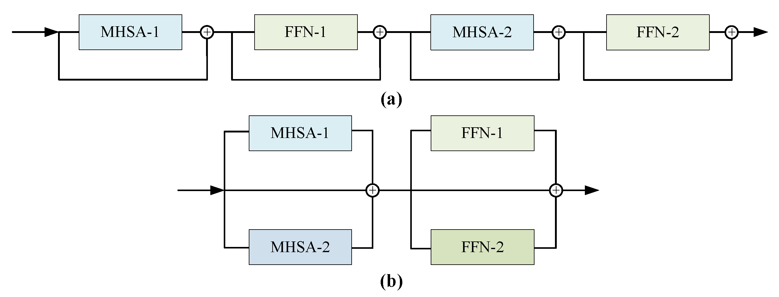
Parallel encoder. The idea of parallel structure is introduced to implement an parallel encoder. It can still have a relatively low depth when superimposed with multiple encoders during training, thus achieving a lower latency and making it easier to optimize. Consequently, the speed of training and prediction is accelerated and good training results can be achieved even on less powerful personal platforms.
(3)
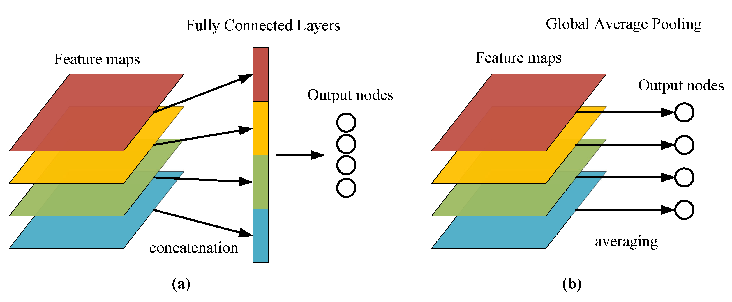
Global average pooling. The global average pooling (GAP) method is used as a substitute for class embedding. A GAP layer is added after the encoder and the average of all the pixels in the feature maps of each channel is taken to give an output. This operation is simple and effective, does not increase additional parameters, and avoids over-fitting. It summarizes spatial information and is more stable to spatial transformations of the input.
The remaining sections of this article are organized as follows. Section 2 provides a brief introduction to the relevant technical background and describes in detail the specific improvements proposed by our method. In Section 3, the experimental results are presented and analyzed comprehensively. Finally, Section 4 concludes the study and offers prospects for future works.

2. The Proposed Method

As input data for the method proposed in this paper, the initial form of the PolSAR data is a 9-D real vector [30]: [ T 11 , T 22 , T 33 , Re [ T 12 ] , Im [ T 12 ] , Re [ T 13 ] , Im [ T 13 ] , Re [ T 23 ] , Im [ T 23 ] ] , where Re [ ] and Im [ ] denote real and imaginary parts, respectively. Its rows represent the feature dimensions, while columns indicate the total number of pixels in the image. The overall structure of the proposed method is illustrated in Figure 1. First of all, we extract pixel-centric neighborhoods of the PolSAR data as image patches of the same size, which serve as the initial input to the model. These image patches are then transformed into 1-D token vectors through mixed depthwise convolution tokenization, without additional class and position embeddings. Moreover, a multi-layer parallel encoder with two branches extracts global information from the input data and obtains the importance weights of each token vector relative to others. Finally, a global average pooling layer is applied to output the features of each class. After incorporating a softmax classifier, pixels can be classified into specific categories and the final output results are obtained. These improvements are described in more detail below.

2.1. Mixed Depthwise Convolution Tokenization

CNNs have been widely used in image classification [31,32,33], segmentation [34,35,36], detection [37,38,39,40] and many other applications [41,42,43,44]. The latest design trend is to improve accuracy or efficiency. Following this trend, depthwise convolutions have become more prevalent in CNNs, such as MobileNet [45], ShuffleNet [46], NASNet [47], etc. Different from conventional convolutions, depthwise convolutions apply the kernel separately to each channel, thereby reducing the computational cost by a factor of c, where c is the number of channels. When designing convolutional networks with depthwise convolutional kernels, the kernel size is an important factor but is often overlooked. Traditionally, a simple 3 × 3 kernel is used, but recent research indicates that larger kernel sizes such as 5 × 5 and 7 × 7 kernels can probably improve the accuracy and efficiency of the model. Tan et al. [48] systematically studied the impact of kernel size and found that a single kernel size is limited. On this basis, the MixConv was proposed, which mixes different kernel sizes in a single convolutional operation, making it easy to capture different patterns at different resolutions. Figure 2 shows the structure of MixConv. It divides the channels into several groups and applies different kernel sizes to each group of channels.
ViT splits the original image into equally sized patches and treats them as words in the text. Since the standard transformer receives token embeddings of 1-D sequences as input, a learnable linear projection is utilized to flatten the patches and map to D dimensions. The processed patches are referred to as patch embeddings, where D is a constant latent vector size that is used throughout all of the ViT layers. To simplify the image representation output by the encoder, ViT introduces a class token by adding a learnable class embedding to the previous patch embeddings. In addition, ViT adds a trainable 1-D position embedding to the patch embeddings to preserve position information. The resulting sequence of patch embedding vectors containing both class and position embeddings is applied as the input to the encoder. During training, the class embedding interacts with each patch embedding to obtain the image representation and serves as the output of the encoder. A classification head is then connected to obtain the final output categories of the model. However, the additional class embedding increases both computational and parameter requirements, while the position embedding fixes the sequence length and constrains the feature information to a immovable scale. To address these issues, we implement tokenization with a modified MixConv. During tokenization, the receptive field of the model is effectively expanded to capture data information at different levels by employing convolution kernels of various sizes. Moreover, tokenization serves as a feature extraction process, where the resulting multi-scale feature maps produced by different receptive fields are presented as input to the encoder. Such tokenization enriches the training data and allows the input resolution to no longer be strictly limited by the preset patch size. Furthermore, the convolution blocks can also be stacked and further down-sampled, even facilitating the removal of position embedding in the model [49]. The implementation details are described below.
As shown in Figure 3, PolSAR patches of size m × m × 9 are first extracted around the center pixels, and these patches are then used as the input data for processing. Since ViT only accepts a sequence of token embeddings, tokenization is essential to transform the 3-D image patches and map them to 2-D patch embeddings. Firstly, the input image patches are grouped according to the number of output channels, with an average division method selected such that d channels are equally divided into 3 groups, denoted as G 1 , G 2 , and G 3 , respectively, where G 1 + G 2 + G 3 = d and d refers to the dimension of the 2-D patch embeddings. For each group, convolution operations are performed with kernels of sizes [ 3 × 3 , 5 × 5 , 7 × 7 ] and a stride of 3, producing feature maps of the shape m 3 , m 3 , d . After passing through a max-pooling layer with a size of 3 × 3 and stride of 1, the original PolSAR patch is split into N 2 feature patches of shape m N , m N , 9 . Eventually, each feature patch is flattened along the spatial dimension to form ( m N · m N · 9 ) -D vectors. These vectors are stacked to reconstruct the input from R m × m × 9 to R N 2 × ( m N · m N · 9 ) , which completes the tokenization process. These vectors are called patch embeddings and serve as input to the subsequent parallel encoder. Unlike the mainstream ViT model [26], class embedding and position embedding are not employed in this work. The class embedding can be replaced by a GAP operation. Furthermore, the classification task does not focus on the location information in the image and there is no strict positional relationship between the pixels in the input PolSAR image patches [50]. Therefore, these two learnable parameters are removed.

2.2. Parallel Encoder

In ViT, the encoder architecture follows the standard transformer structure, consisting of multi-head self-attention (MHSA) and multi-layer perceptron (MLP) layers [25]. Layer normalization (LN) is applied before each layer and residual connection is applied after each layer. The MLP layer contains two layers with Gaussian error linear unit (GELU) [51] activation functions. Compared with CNNs, ViT has fewer image-specific biases as only the MLP layers are local and translation-invariant. Whereas, the MHSA operates globally and utilizes 2-D neighborhoods rarely. In addition, the position embedding is initialized without 2-D position information about the image patches, which requires the model to learn the spatial relationships for all of the image patches from scratch. ViT treats the image as a sequence of image patches and processes them with the transformer architecture that is used in NLP. The strategy is simple and scalable and has shown significant performance gains when combined with pre-training on large data sets. Consequently, ViT achieves state-of-the-art results on many image classification datasets [25]. The overall structure of the ViT model is shown in Figure 4 below.
In recent years, transformer architecture has made a significant impact on the design of the computer vision field. Many architectures [52,53,54,55,56] have directly inherited some designs from transformers or have been inspired by their latest discoveries. Despite the significant progress made by transformers, there is still considerable work to be done in optimizing how they design and train. In neural network architecture design, there is often a debate about how to balance width and depth. Since the introduction of residual networks [57], the obstacles of optimization for deep networks have been significantly reduced. As a result, neural networks have evolved in a deeper direction. However, some studies have shown that shallower networks have lower latency and are easier to optimize [58,59].
The original ViT encoder consists of a series of layers, including normalization layers, multi-head self-attention layers, feed-forward network (FFN) layers, residual structures, etc. All of these layers connected in a fixed order, which results in an ever-growing network depth as the number of encoders continues to increase. Such a design makes the model more powerful but also increases the computational load. Therefore, Touvron et al. [60] proposed a parallel ViT approach by duplicating matching blocks to parallelize the architecture, which can be achieved for any number of parallel blocks. Then, a wider and shallower architecture was created with the same number of parameters and calculations. Depending on the implementation, the design allows for more parallel processing, simplifies the optimization process, and can reduce latency. The idea of shallow networks is adopted by designing the encoder with a parallelized structure, which maintains a relatively low depth even when multiple encoders are stacked for training. Therefore, the proposed method can achieve lower latency and better optimization effects. When trained on platforms with lower computational power, the model produces a good result which demonstrates its applicability.
To capture the long-range interactions between pixels in PolSAR image patches, it is necessary to obtain importance weights for each pixel relative to other pixels. The self-attention mechanism is the main way to accomplish that goal. For each element in the input sequence X R N × D , it is mapped into three variables with the specific dimensions query q, key k, and value v by a learnable linear projection matrix W q k v . The importance weight of this element relative to other elements is obtained by calculating the weighted sum of all values v in the sequence. The attention weights matrix A i j is based on the pairwise similarity between two elements in the sequence and their respective representations of query q i and key k j .
[ q , k , v ] = X W q k v W q k v R D × 3 D h ,
A = softmax q k T D h A R N × N ,
SA ( X ) = A v .
MHSA is an extension of SA. When the input patches are embedded, they are linearly projected into queries and keys of dimensions d k , and values of dimensions d v . These queries, keys, and values are then transformed by h groups of different learnable linear projections. Next, these h sets of transformed queries, keys, and values are processed in parallel through attention pooling. Finally, the outputs of these h attention pooling operations are concatenated together and transformed by another learnable linear projection to produce the final output. This design is referred to as multi-head self-attention, where each of the h outputs of the attention pooling is referred to as a head. If these queries, keys, and values are packed into matrices Q, K, and V, respectively, the output matrix can be represented as:
MHSA ( Q , K , V ) = Concat ( h 1 , , h h ) W O
h i = SA i ( Q W i Q , K W i K , V W i V )
where W i Q R d m o d e l × d k , W i K R d m o d e l × d k , W i V R d m o d e l × d v , and W O R h d v × d m o d e l are parameter matrices for the linear projections. The FFN consists of two fully connected layers (FC) and a GELU activation function, which can be represented as:
FFN ( x ) = max ( 0 , x W 1 + b 1 ) W 2 + b 2
Therefore, the original ViT encoder can be represented as follows:
x l + 1 = x l + MHSA l ( x l ) , x l + 1 = x l + 1 + FFN l ( x l + 1 ) ,
x l + 2 = x l + 1 + MHSA l + 1 ( x l + 1 ) , x l + 2 = x l + 2 + FFN l + 1 ( x l + 2 ) ,
where MHSA l ( ) and MHSA l + 1 ( ) represent MHSA residual blocks, and FFN l ( ) and FFN l + 1 ( ) represent FFN residual blocks. This series of operations can be replaced by a set of parallel structures:
x l + 1 = x l + MHSA l , 1 ( x l ) + MHSA l , 2 ( x l )
x l + 2 = x l + 1 + FFN l , 1 ( x l + 1 ) + FFN l , 2 ( x l + 1 )
For a given number of MHSA and FFN blocks, this will reduce the number of layers by two. As shown in Figure 5, the architecture can be parallelized by pairing identical blocks to achieve any number of parallel blocks. The tokenized patch embeddings are fed into the encoder via three parallel paths to extract global features, which are processed by a number of parallel blocks to obtain the final feature maps.

2.3. Global Average Pooling

When a convolutional neural network is applied to a classification task, the feature map of the last convolutional layer in the network is usually vectorized and mapped to the sample label space by a fully connected (FC) layer, and finally, the final output class is obtained by a softmax classifier [61,62]. Such a structure treats the convolutional layers as feature extractors that can be flexibly applied to different tasks. However, the FC layer has a large number of parameters, which leads to a significant increase in the computational power of the network. It also tends to cause overfitting and affects the generalization ability of the network. Therefore, global average pooling [63] is proposed to replace the FC layer to solve the above problem. As shown in Figure 6, unlike traditional CNNs that add FC layers at the end of the network, GAP takes the average of each feature map and feeds the resulting vector directly into the softmax classifier to obtain the category output. By emphasizing the correspondence between feature maps and categories, GAP is more suitable for convolutional structures and easily interprets feature maps as category confidence maps. In addition, GAP is simple and effective. It does not add any additional parameters, which can prevent overfitting. Furthermore, the spatial information is summed to improve the stability of the model to the input spatial transformation.
In the original ViT model, the class embedding was trained together with other features as part of the global interaction characteristics of ViT. As a result, the trained class embedding can be used as the final output of the model. As the learnable class and positional embeddings are removed in the tokenization process, it is impossible to obtain feature representations of the original data through class embedding. Therefore, a GAP layer is added after the parallel encoder to replace the class embedding. By adding a GAP layer after the parallel encoder, the mean value of all pixels in each channel of the feature map is calculated to obtain one output per feature map. A softmax classification head is connected at the end of the model, which consists of an MLP layer, and the final classification task is achieved by using this classification head to obtain the corresponding category.

3. Experimental Analysis and Results

3.1. Datasets Description

(1)
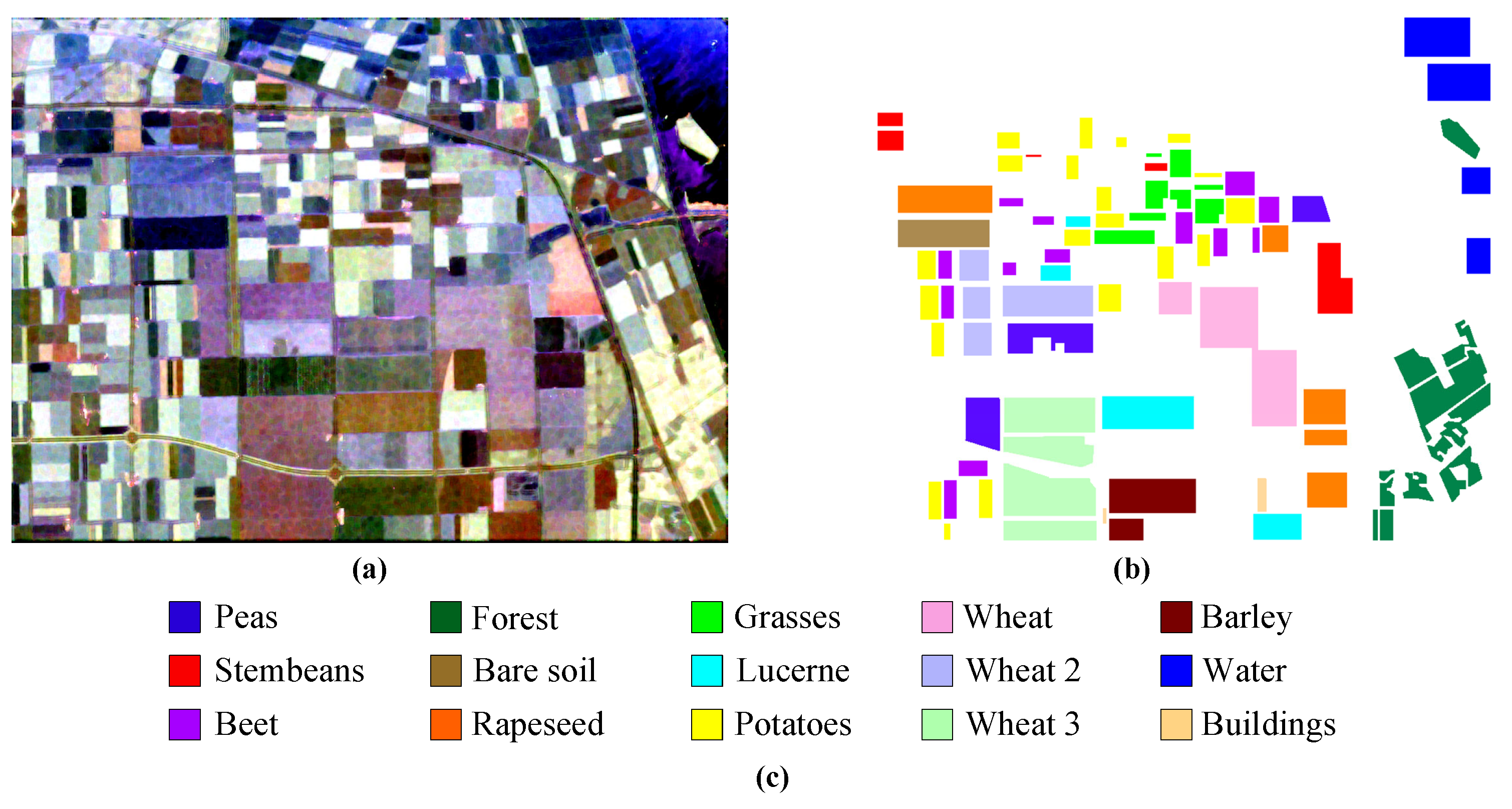
AIRSAR Flevoland: The Flevoland image is a 750 × 1024 subimage of the L-band multi-view PolSAR dataset acquired by the AIRSAR platform on 16 August 1989. The ground resolution of the image is 6.6 m × 12.1 m, and it includes 15 kinds of ground objects, each represented by a unique color. Figure 7a illustrates the Pauli map and Figure 7b shows the ground truth map of the dataset. Figure 7c shows the corresponding ground truth map and legend of the dataset, which consists of 167,712 labeled pixels [64].
(2)
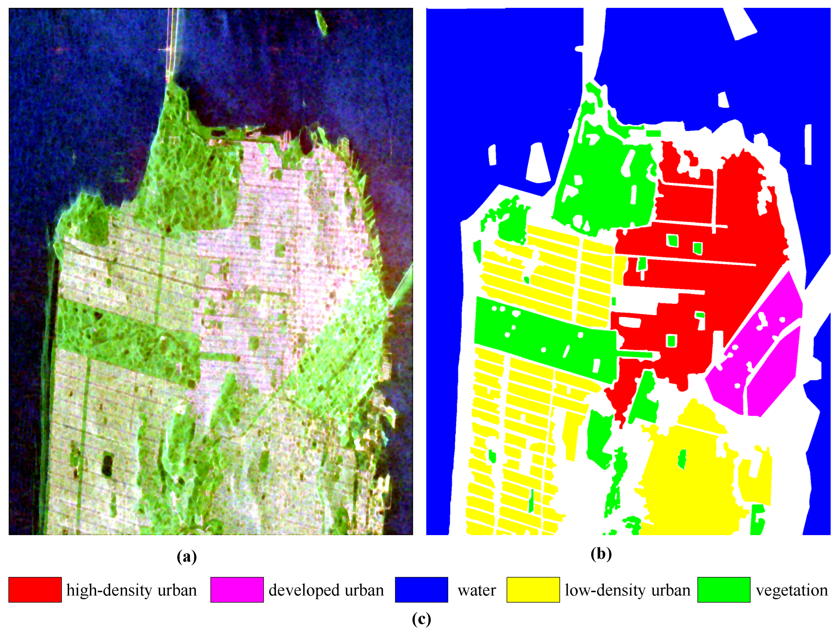
RADARSAT-2 San Francisco: The second dataset is a San Francisco Bay Area image with C-band acquired by the RADARSAT-2 satellite. Figure 8a displays the PauliRGB image of the selected scene with a size of 1380 × 1800, which primarily contains five land cover types: high-density urban areas, water, vegetation, developed urban areas, and low-density urban areas. Figure 8b shows the ground truth map consisting of 1804087 pixels with known label information. Figure 8c respectively show the corresponding ground truth map and the legend explaining the land cover types [65].

3.2. Experimental Setup

The experiments were conducted on a personal laptop computer with the model Legion Y9000P IAH7H, equipped with an NVIDIA GeForce RTX3060 Laptop GPU with 6 GB of graphics memory. The proposed method was implemented using the PyTorch-GPU deep learning framework with PyTorch version 1.11.0 and CUDA version 12.0. Specific details of the experimental setup will be discussed in the following sections.
Since the input for ViT is in image format, a neighborhood with a size of 14 × 14 is extracted centered on pixel. Therefore, the value of the input space size m is set to 15. The MixConv kernel sizes are set to ( 3 , 5 , 7 ) , and the number of output channels d is set to 225. The computation times of the SA, i.e., the number of heads, are set to 4, with the dimension of each head d h set to 76. The number of parallel branches is set to 2, and the depth of the parallel encoder, i.e., the number of parallel blocks, is set to 3. The output of each MHSA and FFN layer in parallel branches is connected to its input through a residual connection. The hidden node numbers in the FC layer of the FFN are set to 900, and the residual structure is also used. Layer normalization is applied before each layer of the parallel encoder to accelerate convergence.
The Flevoland and San Francisco datasets have 167,712 and 1,804,087 labeled data, respectively. For different dataset experiments, 375 labeled data from each category (3.35% and 0.1% of the labeled data in the Flevoland and San Francisco datasets, respectively) are randomly selected for training and validation, while the remaining labeled data are used for testing. To better measure the model’s performance, 5-fold cross-validation is used for training. During training, each model in the 5 folds is trained for 150 epochs with a batch size of 256. The Adam optimizer is used and the initial learning rate is set to 0.001. The loss function is the original cross-entropy loss function in ViT. Moreover, class balance is ensured in each subset of data for each fold. By testing on labeled data and selecting the fold with the highest overall accuracy (OA) among the 5-fold models, the best-performing fold is chosen as the final training model for subsequent result prediction.
To further demonstrate the effectiveness of the proposed method, several PolSAR image classification methods based on CNN or ViT are selected and tested in the following experiments. The CNN-based methods included CV-FCN [66], CV-MLPs [67], and CV-3D-CNN [68]. The ViT-based methods included SViT [27], and PolSARFormer [29], for a total of 5 methods used in the comparative experiments. To ensure the experimental effectiveness of the comparison methods, each comparison method is set up and trained in detail according to the parameters specified in its paper.

3.3. Classification Results

The experimental results on the two datasets are shown in Table 1 and Table 2 and the predicted classification results for all data are shown in Figure 9 and Figure 10. The bolded numbers in both tables indicate the best indicator results in the comparison methods. The colors in both figures are consistent with the meaning indicated by the legend of the corresponding dataset. The experimental results demonstrate that the proposed method can achieve good test accuracy and prediction performance with a relatively small amount of training data. Furthermore, both the training and prediction time are significantly reduced compared with other methods. The following is a detailed discussion of the classification results for each of the datasets, where the training time for the proposed method includes a 5-fold cross-validation training.

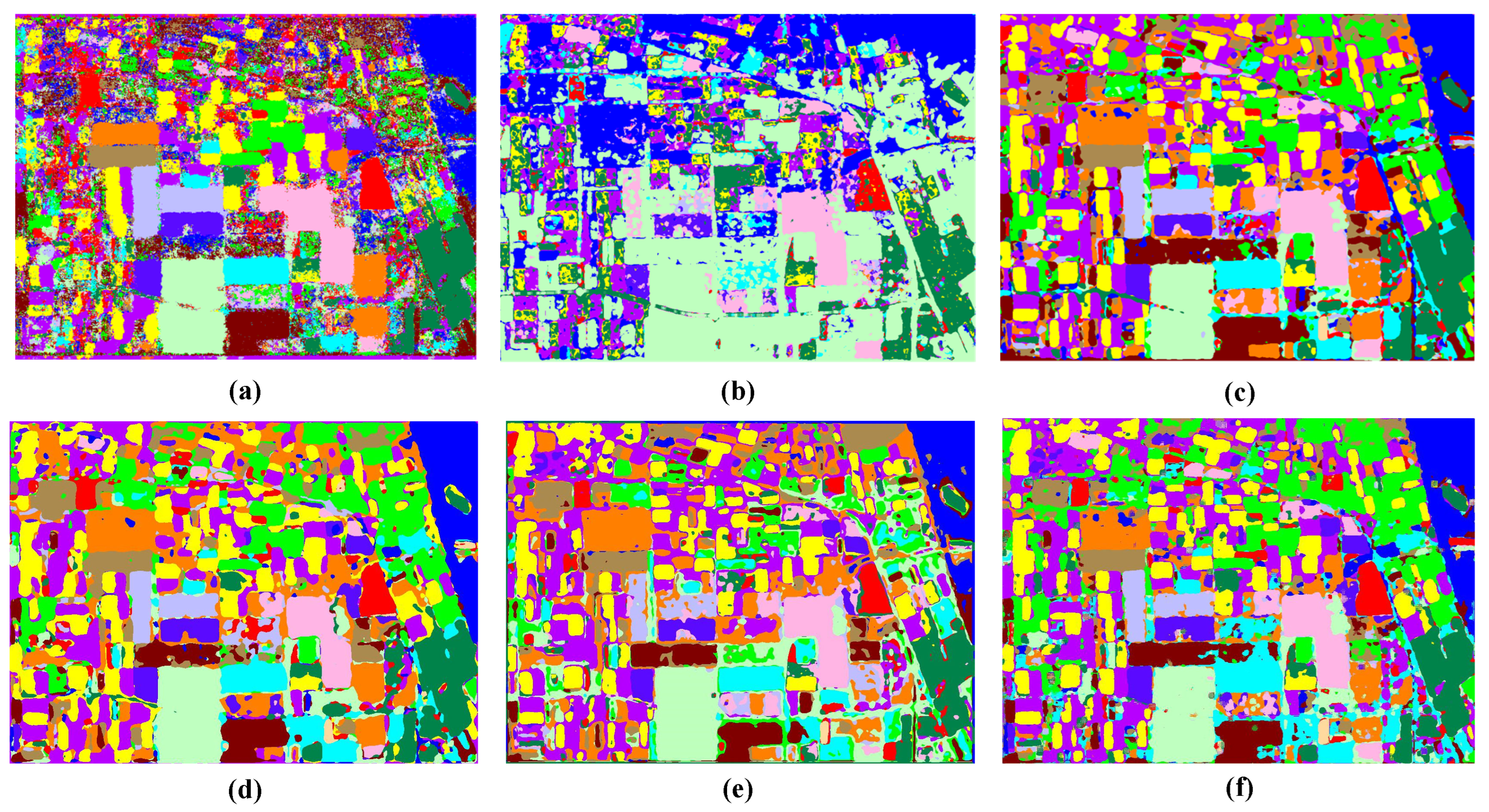
3.3.1. Experimental Results on The AIRSAR Flevoland Dataset

It can be observed from Table 1 that among the CNN-based methods, the CV-FCN method has the highest OA (99.39%), AA (98.98%) and Kappa (99.33%). However, its training time is excessively long at 9034.43 s. The experimental results of the CV-MLPs method are not acceptable compared with other methods. Among the 15 land types, the testing accuracy of four classes, grass, barley, bare doil, and buildings is 0. This indicates that the representation learning ability of this method on the AIRSAR Flevoland dataset is poor and it is not competitive. The CV-3D-CNN method has shown good performance with an OA of 99.01%, AA of 98.94% and Kappa of 98.92%. However, its prediction time (1856.65 s) is the longest of all methods. Among the ViT-based methods, the SViT method also achieves good performance with an OA of 98.62%, AA of 98.49% and Kappa of 98.43%. However, its training time (4294.07 s) and prediction time (85.97 s) are not advantageous. The PolSARFormer method does not have significant advantages in terms of accuracy, and its training and prediction times are too long compared with other methods. The proposed method demonstrates high-level performance in OA (97.90%), AA (97.97%), and Kappa (97.71%). Moreover, it shows strong advantages in terms of both training and prediction time. The training time is only 482.52 s and the prediction time is only 21.93 s.
Figure 9 displays the predicted results of different classification methods on the Flevoland image. It can be seen from Figure 9a that the CV-FCN method can make good predictions on the labeled data but there are irregular and noisy results on the unlabeled part. It has significant overfitting and does not achieve the desired effect. In Figure 9b, it can be observed that the classes of grass, barley, bare soil, and buildings cannot be clearly perceived in the prediction map, while water and wheat 3 occupy most of the image space. It indicates that the CV-MLPs method performs poorly on this dataset, with most regions showing prediction errors. The results of each class in Figure 9d are relatively pure with fewer instances of other categories. However, its classification boundaries are irregular with obvious stickiness. Figure 9e shows slightly worse results. The classification boundaries are unclear and many cases of marginal parts are predicted to be other categories. The prediction results in Figure 9c,f are relatively good and can also provide positive category judgments for the unlabeled part. From some details, it can be seen that the proposed method performs marginally worse than the CV-3D-CNN method in some local classifications. However, the proposed method achieves 100% accuracy in the classification of the bare soil class. Meanwhile, it has an advantage in the prediction results of the building class compared with all other comparison methods. In conclusion, the subjective evaluation of the predicted images based on the corresponding image ground truth and the PauliRGB image leads to the same conclusion as the objective evaluation.

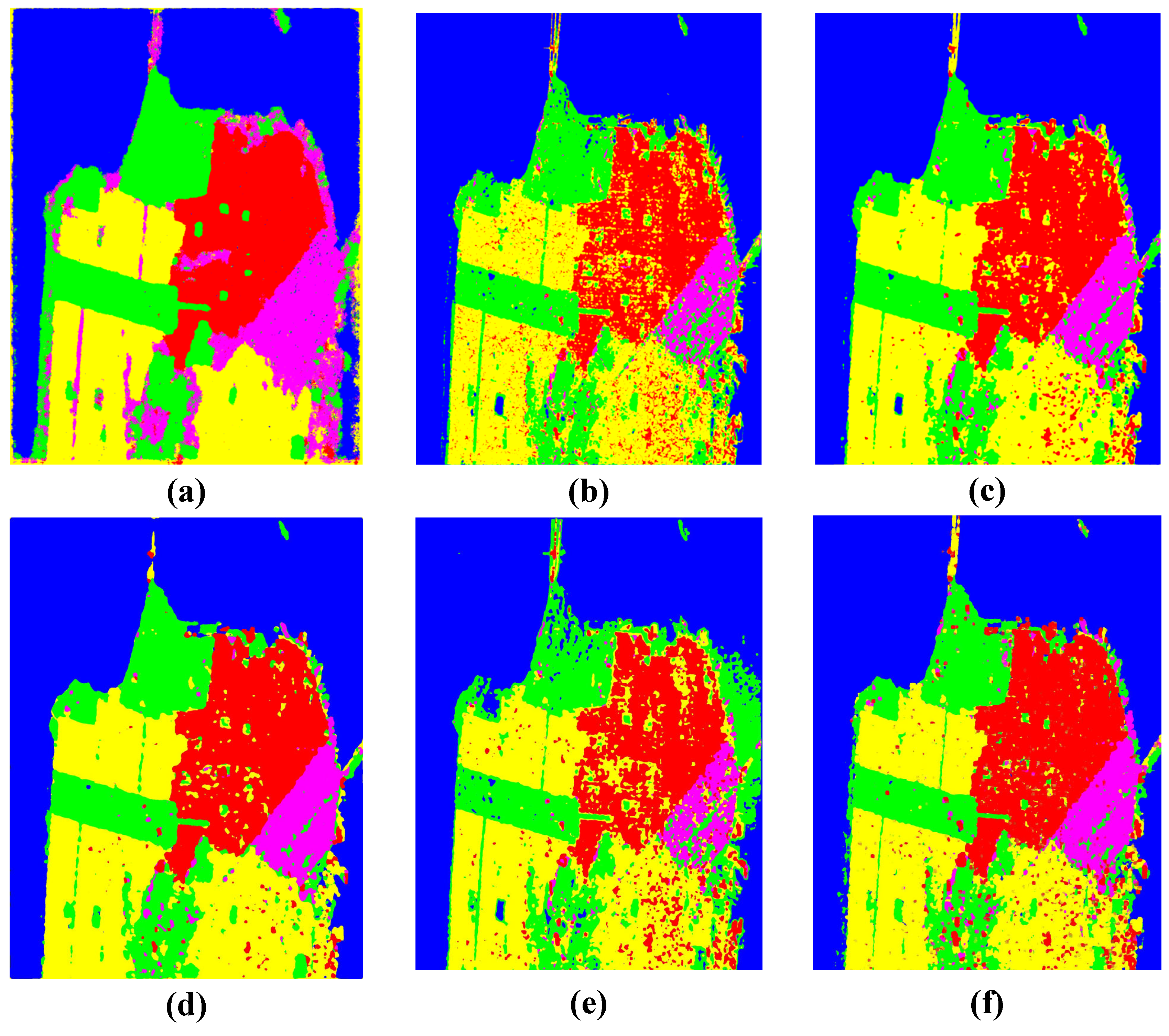
3.3.2. Experiment Results on The RADARSAT-2 San Francisco Dataset

The experiment results in the Table 2 show that the CV-FCN method still achieves the highest OA (99.28%), AA (98.80%), and Kappa (99.02%) among the CNN-based methods. However, it requires a training time of up to 8227.01 s. The CV-MLPs method exhibits a good performance on this dataset. However, its accuracy is low for the vegetation, high-density urban, and low-density urban classes, resulting in a relatively low overall accuracy. The performance of the CV-3D-CNN method on this dataset is worse than on the AIRSAR Flevoland dataset. Not only all three indicators OA (96.85%), AA (95.39%), and Kappa (95.47%) decrease, but also both training time (4865.09 s) and predicting time (12,210.48 s) increase dramatically. This indicates that the CV-3D-CNN method performs less favorably when dealing with large amounts of data. Among the ViT-based methods, the SViT method achieves high accuracy and has advantages in terms of training time (1506.58 s) and prediction time (338.28 s) compared with CNN-based methods. The PolSARFormer method has the lowest accuracy of all the methods used in the experiment. It is not competitive compared with other methods with a training time of 77593.12 s and prediction time of 6038.70 s. The proposed method achieves impressive results in terms of OA (96.77%), AA(94.84%), and Kappa (95.35%). Furthermore, both the training and prediction time are significantly reduced.
Figure 10 illustrates the prediction results of different classification methods on the San Francisco image. According to the predicted image in Figure 10a, the CV-FCN method is the only one with prediction errors at the outer boundary. It is difficult to clearly distinguish the specific shape of the boundary between water and land. In addition, its prediction of the developed urban category is too aggressive, resulting in a wider distribution of this category. The prediction results in Figure 10b are not pure for each category. Figure 10e has relatively poor prediction results. It has more prediction errors at the boundary of water and land, where vegetation at the edge is misclassified as water or the opposite. There is too much of the phenomenon of being predicted as another category in each category area. The predicted results in Figure 10c,d,f are relatively good. Among them, the image in Figure 10d is purer with fewer classification errors in each category. Figure 10c,f are slightly inferior to Figure 10d. However, the difference is not significant. In summary, subjective visual evaluation of the predicted image leads to the same conclusion as the objective evaluation, which again confirms the feasibility of the proposed method.
On the AIRSAR Flevoland dataset, CV-3D-CNN outperforms other comparative methods when all factors are considered. The proposed method achieves a remarkable increase of approximately 5 times in training speed and 85 times in prediction speed compared with the CV-3D-CNN. Meanwhile, it exhibits some minor decrease of 1.11%, 0.97%, and 1.21% in terms of OA, AA, and Kappa, respectively. Similarly, on the RADARSAT-2 San Francisco dataset, the SViT performs best among other comparative methods. The proposed method shows a respective decrease of 1.21%, 1.92%, and 1.75% in OA, AA, and Kappa compared to the SViT. However, there is an acceleration of about 9 times in training speed and 4 times in prediction speed.
The experimental results on both datasets demonstrate that the proposed method achieves good test accuracy and prediction performance with relatively small amounts of training data. There is a significant reduction in training and prediction time in comparison to other methods. Sacrificing a slightly lower accuracy for considerably improved training and prediction speed leads to excellent time efficiency in practical applications. However, when other methods use the same amount of data as the proposed methods, some methods cannot be trained well and fail to learn useful features that cause a decrease in classification accuracy. Some other methods are slower and have longer training time and prediction time.

4. Discussion

4.1. Ablation Experiments

To verify the effectiveness of each mechanism introduced in the proposed method, ablation experiments are performed on the AIRSAR Flevoland dataset. Experimenting with the three mechanisms will generate many control experiments. Due to time and space constraints, only two mechanisms, mixed depthwise convolution tokenization and parallel encoder, will be discussed here. In the ablation experiments, five metrics are chosen as the judging standard, namely, overall accuracy (OA), training time, prediction time, number of Floating Point Operations (FLOPs), and number of parameters (Params). The first three of the metrics are the same as used in the above comparison experiments to visualize the actual effect of each control group in the ablation experiments. FLOPs is used to measure the model computational complexity and can indirectly measure the model speed. Params is the total number of parameters to be trained in the network model, which is used to measure the size of the model. Table 3 shows the results of the ablation experiments.
To facilitate the description of the experimental results, each experiment is numbered in the table. Experiment (1) is first performed on the original ViT, and the results of this experiment are used as the baseline for the overall ablation experiments. As can be seen from Table 3, the original ViT can achieve a high level of OA on the PolSAR image classification. However, its training time and prediction time are longer, which can also be seen from its FLOPs and Params corresponding to the correlation. The FLOPs of the original ViT is as high as 1703.363 M and the Params also reaches 85.241 M, indicating that its computational and parametric quantities are large. Thus, its direct application to PolSAR image classification has problems such as model complexity and parameter redundancy. Experiment (2) shows a slight decrease in OA after replacing the ViT tokenization process with the mixed depthwise convolution tokenization mechanism introduced in this paper. However, the training time and prediction time are dramatically reduced, and the number of computations and parameters are significantly reduced. The results of this experiment demonstrate the effectiveness of the mixed depthwise convolution tokenization mechanism, which is consistent with the theory described in the previous section. Experiment (3) changes the encoder to the parallel encoder used in the proposed method on the basis of ViT. From the experimental results, it can be seen that adding only the parallel encoder has a large impact on the OA of the model, reducing the accuracy by 2.51%. It is due to the fact that the width network shows a weaker learning ability at a shallower network level compared to the depth network. However, as the number of network levels increases, the width network will have the same model performance as the depth network, and it is easier to optimize than the depth network. The addition of parallel encoder is also able to significantly reduce the training time and prediction time, and the reduction is slightly larger compared to experiment (2). Moreover, the number of computations and parameters are significantly reduced. Experiment (3) shows that the introduction of parallel encoder can effectively reduce the training time and prediction time, as well as the computational and parametric quantities, in accordance with the above theory. Experiment (4) introduces both mixed depthwise convolution tokenization and parallel encoder mechanisms. From the results, it can be seen that the accuracy has improved compared to experiment (3) where only parallel encoder is introduced, and basically reaches the same level as ViT. The training time and prediction time are between experiment (2) and experiment (3), and the computation and the number of parameters are the same as those in experiment (2), which are in accordance with the theoretical requirements. For experiment (5), i.e., the test results of the proposed method MCPT are basically the same as experiment (4) with slight optimization. It shows that the overall impact of GAP on the proposed method is smaller than the other two mechanisms. Therefore, it is not discussed in detail here.
In conclusion, the results of the ablation experiments demonstrate the effectiveness of the three mechanisms introduced in this paper. It is further verified that the proposed method is able to maintain a high level of accuracy while significantly improving the training speed and prediction speed, reducing the model complexity, and enabling ViT to be better applied to PolSAR image classification tasks.

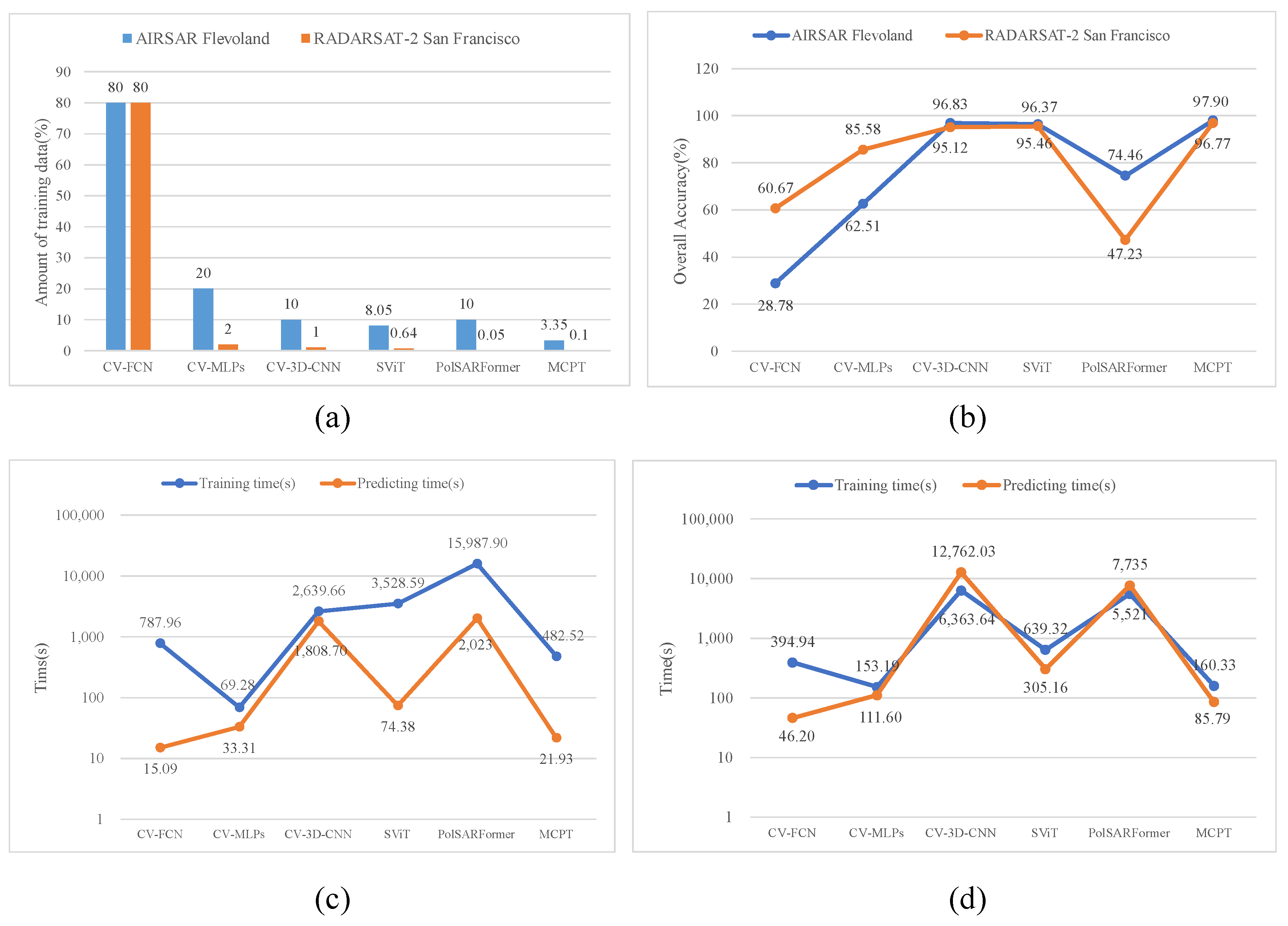
4.2. Impact of Training Data Amount

In deep learning methods, the size of the training data plays an important role in the final effect of the model. Figure 11a shows the amount of training data used by all comparison methods and the proposed method, where the numbers represent the weight of the amount of training data used by the different methods on the two datasets relative to all labeled data. As can be seen from Figure 11a, the training data used by the comparison methods are more than those of the proposed method. Among them, the CV-FCN method even uses 80% of the labeled data for training, which enables it to achieve good test results, but also raises the problem of poor prediction of such unlabeled regions as the ones shown in Figure 9a.
When all comparison methods are trained according to the amount of data used in this paper, the results are unsatisfactory. Figure 11b–d present the results of different comparison methods trained on the two datasets according to the amount of data used in this paper. Where Figure 11b shows the OA of the test on the two datasets. It can be seen that after reducing the amount of training data, the OA of the comparison methods for testing on both datasets is lower than that of the proposed method. The results show that the reduction in the amount of training data affects the accuracy performance of the comparison methods. Meanwhile, it is demonstrated that the proposed method can achieve a high level of accuracy performance when using a small amount of training data. Figure 11c,d shows the training time and prediction time performance on the AIRSAR Flevoland and RADARSAT-2 San Francisco datasets, respectively. From the two figures, it is observed that the proposed method in this paper still shows a strong advantage in training time and prediction time when the same amount of data is used.
The impact of the amount of training data on the different methods can be illustrated in the figures above. Although the degree of impact varies, more or less all bring about a loss of accuracy. The effectiveness of the proposed method can be verified by the fact that the proposed method can achieve a high level of overall accuracy with fewer training data and less training time and prediction time. While using the same amount of training data as the proposed method, the results of the comparison methods all become worse to different degrees, which further verifies the effectiveness of the proposed method.

4.3. About PolSAR Image Classification Metrics

The commonly used evaluation metrics in PolSAR image classification are overall accuracy (OA), average accuracy per class (AA), and kappa coefficient (Kappa). OA indicates the ratio of the number of correctly classified samples to the number of all samples, and it is used to evaluate the overall performance of the model. AA represents the ratio between the number of correct predictions in each category and the overall number in each category, and ultimately then averages the accuracy of each category for measuring the performance of the model on a given land cover type. The Kappa coefficient is a measure of classification accuracy for consistency testing and is calculated based on the confusion matrix. Its value usually ranges from 0 to 1. Larger values indicate higher consistency and better model classification performance. OA, AA, and Kappa are calculated as follows, respectively:
O A = T P + T N T P + F N + F P + T N
A A = R e c a l l i N i
R e c a l l = T P T P + F N
K a p p a = p o p e 1 p e
where T P denotes true positive, F N denotes false negative, F P denotes false positive, and T N denotes true negative; i denotes the category and N i denotes the number of categories; R e c a l l denotes the recall rate, i.e., the ratio of the number of correctly classified positive samples to the number of positive samples; p o denotes the overall classification accuracy, a 1 , a 2 , , a c denotes the number of true samples per class, b 1 , b 2 , , b c denotes the number of predicted samples per class, and n denotes the total number of samples, then p e can be expressed as:
p e = a 1 × b 1 + a 2 × b 2 + + a c × b c n 2
From the above three metrics, it can be seen that AA contains the meaning represented by recall, and recall is mostly used for binary classification. However, this paper mainly focuses on multi-classification tasks, so recall is not a good measure of the effect of the model used in this paper. As for Kappa, it is calculated from the confusion matrix and its result already contains the information about the confusion matrix. Therefore, the performance of the PolSAR image classification effect can be basically evaluated completely using these three metrics.

5. Conclusions

By investigating the limitations of CNN application on PolSAR image classification and exploring in depth the different implementations of ViT for the tasks, this paper proposes an MCPT model based on ViT for PolSAR image classification. The proposed model employs a mixed depthwise convolution for tokenization and parallel encoders to learn representations of PolSAR images. In addition, the class enbedding is replaced by a GAP operation and the position embedding is removed. All of these improvements reduce the need for extensive training data and computational complexity. Moreover, the model significantly enhances training and prediction speed while maintaining a high level of accuracy. The experimental results on both datasets demonstrate that the proposed method achieves good test accuracy and prediction performance with relatively small amounts of training data. This results in sacrificing a slightly lower accuracy for considerably improved training and prediction speed. Future research will focus on proposing a more reasonable ViT-based classification method that improves classification accuracy while maintaining the existing training and prediction speed. In addition, it is also a good research direction to better combine CNN with ViT to extract both local and global features in PolSAR images.

Author Contributions

Conceptualization, W.W.; Data curation, J.W. and B.L. (Boyuan Liu); Formal analysis, W.W.; Funding acquisition, J.W. and C.W.; Methodology, W.W.; Project administration, B.L. (Bibo Lu); Resources, B.L. (Bibo Lu); Software, W.W.; Supervision, J.W. and Y.Z.; Validation, C.W.; Visualization, B.L. (Boyuan Liu); Writing—original draft, W.W.; Writing—review and editing, J.W. and B.L. (Bibo Lu). All authors have read and agreed to the published version of the manuscript.

Funding

This research was funded partly by the National Natural Science Foundation of China under Grant 62201201; the Doctoral Foundation of Henan Polytechnic University under Grant B2022-15; the Henan Provincial Science and Technology Research Project under Grant 232102211019; and the Key Research Project Fund of Institution of Higher Education in Henan Province under Grant 23A520029.

Data Availability Statement

The Flevoland dataset acquired by NASA/JPL AIRSAR is openly available in the official website of AIRSAR at https://airsar.jpl.nasa.gov/ (accessed on 16 August 1989). The San Francisco dataset acquired by CSA RADARSAT-2 is openly available in the website at https://ietr-lab.univ-rennes1.fr/polsarpro-bio/san-francisco/ (accessed on 9 April 2008).

Acknowledgments

The authors would like to thank the anonymous reviewers for their constructive comments and suggestions which strengthened a lot this paper.

Conflicts of Interest

The authors declare no conflict of interest.

Abbreviations

The following abbreviations are used in this manuscript:
ViTVision transformer
MCPTMixed convolutional parallel transformer
SARSynthetic aperture radar
PolSARPolarimetric synthetic aperture image
CNNConvolutional neural network
NLPNatural language processing
SASelf-attention
MixConvMixed depthwise convolution
GAPGlobal average pooling
MHSAMulti-head self-attention
MLPMulti-layer perceptron
LNLayer normalization
GELUGaussian error linear unit
FFNFeed-forward network
FCFully connected
OAOverall accuracy
AAAverage accuracy

References

  1. Chan, Y.K.; Koo, V.C. An introduction to synthetic aperture radar (SAR). Prog. Electromagn. Res. B 2008, 2, 27–60. [Google Scholar] [CrossRef] [Green Version]
  2. Bamler, R. Principles of Synthetic Aperture Radar. Surv. Geophys. 2000, 21, 147–157. [Google Scholar] [CrossRef]
  3. Pasmurov, A.; Zinoviev, J. Radar Imaging Application. In Radar Imaging and Holography; IET Digital Library: London, UK, 2005; pp. 191–230. [Google Scholar] [CrossRef]
  4. Ulander, L.; Barmettler, A.; Flood, B.; Frölind, P.O.; Gustavsson, A.; Jonsson, T.; Meier, E.; Rasmusson, J.; Stenström, G. Signal-to-Clutter Ratio Enhancement in Bistatic Very High Frequency (VHF)-Band SAR Images of Truck Vehicles in Forested and Urban Terrain. IET Radar Sonar Navig. 2010, 4, 438. [Google Scholar] [CrossRef]
  5. Zhang, X.; Jiao, L.; Liu, F.; Bo, L.; Gong, M. Spectral Clustering Ensemble Applied to SAR Image Segmentation. IEEE Trans. Geosci. Remote Sens. 2008, 46, 2126–2136. [Google Scholar] [CrossRef] [Green Version]
  6. Chai, H.; Yan, C.; Zou, Y.; Chen, Z. Land Cover Classification of Remote Sensing Image of Hubei Province by Using PSP Net. Geomat. Inf. Sci. Wuhan Univ. 2021, 46, 1224–1232. [Google Scholar] [CrossRef]
  7. Zhang, L.; Duan, B.; Zou, B. Research Development on Target Decomposition Method of Polarimetric SAR Image. J. Electron. Inf. Technol. 2016, 38, 3289–3297. [Google Scholar] [CrossRef]
  8. West, R.D.; Riley, R.M. Polarimetric Interferometric SAR Change Detection Discrimination. IEEE Trans. Geosci. Remote Sens. 2019, 57, 3091–3104. [Google Scholar] [CrossRef]
  9. Holm, W.; Barnes, R. On Radar Polarization Mixed Target State Decomposition Techniques. In Proceedings of the 1988 IEEE National Radar Conference, Ann Arbor, MI, USA, 20–21 April 1988; pp. 249–254. [Google Scholar] [CrossRef]
  10. Cameron, W.; Leung, L. Feature Motivated Polarization Scattering Matrix Decomposition. In Proceedings of the IEEE International Conference on Radar, Arlington, VA, USA, 7–10 May 1990; pp. 549–557. [Google Scholar] [CrossRef]
  11. Cloude, S. Target Decomposition Theorems in Radar Scattering. Electron. Lett. 1985, 21, 22–24. [Google Scholar] [CrossRef]
  12. Cloude, S.; Pottier, E. An Entropy Based Classification Scheme for Land Applications of Polarimetric SAR. IEEE Trans. Geosci. Remote Sens. 1997, 35, 68–78. [Google Scholar] [CrossRef]
  13. Krogager, E. New Decomposition of the Radar Target Scattering Matrix. Electron. Lett. 1990, 26, 1525. [Google Scholar] [CrossRef]
  14. Parikh, H.; Patel, S.; Patel, V. Classification of SAR and PolSAR Images Using Deep Learning: A Review. Int. J. Image Data Fusion 2020, 11, 1–32. [Google Scholar] [CrossRef]
  15. Wang, H.; Xu, F.; Jin, Y.Q. A Review of Polsar Image Classification: From Polarimetry to Deep Learning. In Proceedings of the IGARSS 2019–2019 IEEE International Geoscience and Remote Sensing Symposium, Yokohama, Japan, 28 July–2 August 2019; pp. 3189–3192. [Google Scholar] [CrossRef]
  16. Chua, L.; Roska, T. The CNN Paradigm. IEEE Trans. Circuits Syst. I 1993, 40, 147–156. [Google Scholar] [CrossRef]
  17. Zhou, Y.; Wang, H.; Xu, F.; Jin, Y. Polarimetric SAR Image Classification Using Deep Convolutional Neural Networks. IEEE Geosci. Remote Sens. Lett. 2016, 13, 1935–1939. [Google Scholar] [CrossRef]
  18. Chen, S.; Tao, C. PolSAR Image Classification Using Polarimetric-Feature-Driven Deep Convolutional Neural Network. IEEE Geosci. Remote Sens. Lett. 2018, 15, 627–631. [Google Scholar] [CrossRef]
  19. Lee, H.; Kwon, H. Going Deeper With Contextual CNN for Hyperspectral Image Classification. IEEE Trans. Image Process. 2017, 26, 4843–4855. [Google Scholar] [CrossRef] [PubMed] [Green Version]
  20. Chen, S.; Li, Y.; Wang, X.; Xiao, S.; Sato, M. Modeling and Interpretation of Scattering Mechanisms in Polarimetric Synthetic Aperture Radar: Advances and Perspectives. IEEE Signal Process. Mag. 2014, 31, 79–89. [Google Scholar] [CrossRef]
  21. Chen, S.; Wang, X.; Sato, M. Uniform Polarimetric Matrix Rotation Theory and Its Applications. IEEE Trans. Geosci. Remote Sens. 2014, 52, 4756–4770. [Google Scholar] [CrossRef]
  22. Yang, C.; Hou, B.; Ren, B.; Hu, Y.; Jiao, L. CNN-Based Polarimetric Decomposition Feature Selection for PolSAR Image Classification. IEEE Trans. Geosci. Remote Sens. 2019, 57, 8796–8812. [Google Scholar] [CrossRef]
  23. Shang, R.; He, J.; Wang, J.; Xu, K.; Jiao, L.; Stolkin, R. Dense Connection and Depthwise Separable Convolution Based CNN for Polarimetric SAR Image Classification. Knowl.-Based Syst. 2020, 194, 105542. [Google Scholar] [CrossRef]
  24. Vaswani, A.; Shazeer, N.; Parmar, N.; Uszkoreit, J.; Jones, L.; Gomez, A.N.; Kaiser, L.; Polosukhin, I. Attention Is All You Need. arXiv 2017, arXiv:1706.03762. [Google Scholar]
  25. Dosovitskiy, A.; Beyer, L.; Kolesnikov, A.; Weissenborn, D.; Zhai, X.; Unterthiner, T.; Dehghani, M.; Minderer, M.; Heigold, G.; Gelly, S.; et al. An Image Is Worth 16 × 16 Words: Transformers for Image Recognition at Scale. In Proceedings of the International Conference on Learning Representations, Kigali, Rwanda, 1–5 May 2023. [Google Scholar]
  26. Han, K.; Wang, Y.; Chen, H.; Chen, X.; Guo, J.; Liu, Z.; Tang, Y.; Xiao, A.; Xu, C.; Xu, Y.; et al. A Survey on Vision Transformer. IEEE Trans. Pattern Anal. Mach. Intell. 2023, 45, 87–110. [Google Scholar] [CrossRef]
  27. Dong, H.; Zhang, L.; Zou, B. Exploring Vision Transformers for Polarimetric SAR Image Classification. IEEE Trans. Geosci. Remote Sens. 2022, 60, 1–15. [Google Scholar] [CrossRef]
  28. Wang, H.; Xing, C.; Yin, J.; Yang, J. Land Cover Classification for Polarimetric SAR Images Based on Vision Transformer. Remote Sens. 2022, 14, 4656. [Google Scholar] [CrossRef]
  29. Jamali, A.; Roy, S.K.; Bhattacharya, A.; Ghamisi, P. Local Window Attention Transformer for Polarimetric SAR Image Classification. IEEE Geosci. Remote Sens. Lett. 2023, 20, 1–5. [Google Scholar] [CrossRef]
  30. Zhang, Z.; Wang, H.; Xu, F.; Jin, Y.Q. Complex-Valued Convolutional Neural Network and Its Application in Polarimetric SAR Image Classification. IEEE Trans. Geosci. Remote Sens. 2017, 55, 7177–7188. [Google Scholar] [CrossRef]
  31. Li, Q.; Cai, W.; Wang, X.; Zhou, Y.; Feng, D.D.; Chen, M. Medical Image Classification with Convolutional Neural Network. In Proceedings of the 2014 13th International Conference on Control Automation Robotics & Vision (ICARCV), Singapore, 10–12 December 2014; pp. 844–848. [Google Scholar] [CrossRef]
  32. Qin, J.; Pan, W.; Xiang, X.; Tan, Y.; Hou, G. A Biological Image Classification Method Based on Improved CNN. Ecol. Inform. 2020, 58, 101093. [Google Scholar] [CrossRef]
  33. Sultana, F.; Sufian, A.; Dutta, P. Advancements in Image Classification Using Convolutional Neural Network. In Proceedings of the 2018 Fourth International Conference on Research in Computational Intelligence and Communication Networks (ICRCICN), Kolkata, India, 22–23 November 2018; pp. 122–129. [Google Scholar] [CrossRef] [Green Version]
  34. Dolz, J.; Gopinath, K.; Yuan, J.; Lombaert, H.; Desrosiers, C.; Ben Ayed, I. HyperDense-Net: A Hyper-Densely Connected CNN for Multi-Modal Image Segmentation. IEEE Trans. Med. Imaging 2019, 38, 1116–1126. [Google Scholar] [CrossRef] [Green Version]
  35. Liu, F.; Lin, G.; Shen, C. CRF Learning with CNN Features for Image Segmentation. Pattern Recognit. 2015, 48, 2983–2992. [Google Scholar] [CrossRef] [Green Version]
  36. Mortazi, A.; Bagci, U. Automatically Designing CNN Architectures for Medical Image Segmentation. In Proceedings of the Machine Learning in Medical Imaging, Granada, Spain, 16 September 2018; Shi, Y., Suk, H.I., Liu, M., Eds.; Lecture Notes in Computer Science; Springer: Cham, Switzerland, 2018; pp. 98–106. [Google Scholar] [CrossRef] [Green Version]
  37. Chandrasegaran, K.; Tran, N.T.; Cheung, N.M. A Closer Look at Fourier Spectrum Discrepancies for CNN-generated Images Detection. In Proceedings of the 2021 IEEE/CVF Conference on Computer Vision and Pattern Recognition (CVPR), Nashville, TN, USA, 20–25 June 2021; pp. 7196–7205. [Google Scholar] [CrossRef]
  38. Chattopadhyay, A.; Maitra, M. MRI-based Brain Tumour Image Detection Using CNN Based Deep Learning Method. Neurosci. Inform. 2022, 2, 100060. [Google Scholar] [CrossRef]
  39. Chauhan, R.; Ghanshala, K.K.; Joshi, R. Convolutional Neural Network (CNN) for Image Detection and Recognition. In Proceedings of the 2018 First International Conference on Secure Cyber Computing and Communication (ICSCCC), Jalandhar, India, 15–17 December 2018; pp. 278–282. [Google Scholar] [CrossRef]
  40. Zhou, Z.; Wu, Q.M.J.; Wan, S.; Sun, W.; Sun, X. Integrating SIFT and CNN Feature Matching for Partial-Duplicate Image Detection. IEEE Trans. Emerg. Top. Comput. Intell. 2020, 4, 593–604. [Google Scholar] [CrossRef]
  41. Bhatt, D.; Patel, C.; Talsania, H.; Patel, J.; Vaghela, R.; Pandya, S.; Modi, K.; Ghayvat, H. CNN Variants for Computer Vision: History, Architecture, Application, Challenges and Future Scope. Electronics 2021, 10, 2470. [Google Scholar] [CrossRef]
  42. Jia, W.; Tian, Y.; Luo, R.; Zhang, Z.; Lian, J.; Zheng, Y. Detection and Segmentation of Overlapped Fruits Based on Optimized Mask R-CNN Application in Apple Harvesting Robot. Comput. Electron. Agric. 2020, 172, 105380. [Google Scholar] [CrossRef]
  43. Ravanbakhsh, M.; Nabi, M.; Mousavi, H.; Sangineto, E.; Sebe, N. Plug-and-Play CNN for Crowd Motion Analysis: An Application in Abnormal Event Detection. In Proceedings of the 2018 IEEE Winter Conference on Applications of Computer Vision (WACV), Lake Tahoe, NV, USA, 12–15 March 2018; pp. 1689–1698. [Google Scholar] [CrossRef] [Green Version]
  44. Xie, W.; Zhang, C.; Zhang, Y.; Hu, C.; Jiang, H.; Wang, Z. An Energy-Efficient FPGA-Based Embedded System for CNN Application. In Proceedings of the 2018 IEEE International Conference on Electron Devices and Solid State Circuits (EDSSC), Shenzhen, China, 6–8 June 2018; pp. 1–2. [Google Scholar] [CrossRef]
  45. Sandler, M.; Howard, A.; Zhu, M.; Zhmoginov, A.; Chen, L.C. MobileNetV2: Inverted Residuals and Linear Bottlenecks. In Proceedings of the 2018 IEEE/CVF Conference on Computer Vision and Pattern Recognition, Salt Lake City, UT, USA, 18–23 June 2018; pp. 4510–4520. [Google Scholar] [CrossRef] [Green Version]
  46. Ma, N.; Zhang, X.; Zheng, H.T.; Sun, J. ShuffleNet V2: Practical Guidelines for Efficient CNN Architecture Design. In Proceedings of the Computer Vision—ECCV, Munich, Germany, 8–14 September 2018; Springer: Cham, Switzerland, 2018; pp. 122–138. [Google Scholar] [CrossRef] [Green Version]
  47. Zoph, B.; Vasudevan, V.; Shlens, J.; Le, Q.V. Learning Transferable Architectures for Scalable Image Recognition. In Proceedings of the 2018 IEEE/CVF Conference on Computer Vision and Pattern Recognition, Salt Lake City, UT, USA, 18–23 June 2018; pp. 8697–8710. [Google Scholar] [CrossRef] [Green Version]
  48. Tan, M.; Le, Q.V. MixConv: Mixed Depthwise Convolutional Kernels. arXiv 2019, arXiv:1907.09595. [Google Scholar]
  49. Hassani, A.; Walton, S.; Shah, N.; Abuduweili, A.; Li, J.; Shi, H. Escaping the Big Data Paradigm with Compact Transformers. arXiv 2022, arXiv:2104.05704. [Google Scholar]
  50. Chen, X.; Xie, S.; He, K. An Empirical Study of Training Self-Supervised Vision Transformers. In Proceedings of the 2021 IEEE/CVF International Conference on Computer Vision (ICCV), Montreal, BC, Canada, 11–17 October 2021; pp. 9620–9629. [Google Scholar] [CrossRef]
  51. Hendrycks, D.; Gimpel, K. Gaussian Error Linear Units (GELUs). arXiv 2020, arXiv:1606.08415. [Google Scholar]
  52. Chen, C.F.R.; Fan, Q.; Panda, R. CrossViT: Cross-Attention Multi-Scale Vision Transformer for Image Classification. In Proceedings of the 2021 IEEE/CVF International Conference on Computer Vision (ICCV), Montreal, BC, Canada, 11–17 October 2021; pp. 347–356. [Google Scholar] [CrossRef]
  53. Chu, X.; Tian, Z.; Wang, Y.; Zhang, B.; Ren, H.; Wei, X.; Xia, H.; Shen, C. Twins: Revisiting the Design of Spatial Attention in Vision Transformers. In Proceedings of the Advances in Neural Information Processing Systems 34, Online, 7 December 2021; Curran Associates, Inc.: New York City, NY, USA, 2021; pp. 9355–9366. [Google Scholar]
  54. Heo, B.; Yun, S.; Han, D.; Chun, S.; Choe, J.; Oh, S.J. Rethinking Spatial Dimensions of Vision Transformers. In Proceedings of the 2021 IEEE/CVF International Conference on Computer Vision (ICCV), Montreal, BC, Canada, 11–17 October 2021; pp. 11916–11925. [Google Scholar] [CrossRef]
  55. Tu, Z.; Talebi, H.; Zhang, H.; Yang, F.; Milanfar, P.; Bovik, A.; Li, Y. MaxViT: Multi-axis Vision Transformer. In Computer Vision—ECCV 2022. ECCV 2022; Avidan, S., Brostow, G., Cissé, M., Farinella, G.M., Hassner, T., Eds.; Lecture Notes in Computer Science; Springer: Cham, Switzerland, 2022; pp. 459–479. [Google Scholar] [CrossRef]
  56. Yang, R.; Ma, H.; Wu, J.; Tang, Y.; Xiao, X.; Zheng, M.; Li, X. ScalableViT: Rethinking the Context-Oriented Generalization of Vision Transformer. In Computer Vision—ECCV 2022. ECCV 2022; Avidan, S., Brostow, G., Cissé, M., Farinella, G.M., Hassner, T., Eds.; Lecture Notes in Computer Science; Springer: Cham, Switzerland, 2022; pp. 480–496. [Google Scholar] [CrossRef]
  57. He, K.; Zhang, X.; Ren, S.; Sun, J. Deep Residual Learning for Image Recognition. In Proceedings of the 2016 IEEE Conference on Computer Vision and Pattern Recognition (CVPR), Las Vegas, Nevada, USA, 27–30 June 2016; pp. 770–778. [Google Scholar] [CrossRef] [Green Version]
  58. Goyal, A.; Bochkovskiy, A.; Deng, J.; Koltun, V. Non-Deep Networks. In Proceedings of the Advances in Neural Information Processing Systems 35, New Orleans, LA, USA, 28 November–9 December 2022. [Google Scholar]
  59. Zhou, J.; Wei, C.; Wang, H.; Shen, W.; Xie, C.; Yuille, A.; Kong, T. Image BERT Pre-training with Online Tokenizer. In Proceedings of the International Conference on Learning Representations, Virtual, 25–29 April 2022. [Google Scholar]
  60. Touvron, H.; Cord, M.; El-Nouby, A.; Verbeek, J.; Jégou, H. Three Things Everyone Should Know About Vision Transformers. In Proceedings of the 17th European Conference, Tel Aviv, Israel, 23–27 October 2022; Avidan, S., Brostow, G., Cissé, M., Farinella, G.M., Hassner, T., Eds.; Lecture Notes in Computer Science. Springer: Cham, Switzerland, 2022; pp. 497–515. [Google Scholar] [CrossRef]
  61. Goodfellow, I.; Warde-Farley, D.; Mirza, M.; Courville, A.; Bengio, Y. Maxout Networks. In Proceedings of the 30th International Conference on Machine Learning (PMLR), Atlanta, GA, USA, 17–19 June 2013; pp. 1319–1327. [Google Scholar]
  62. Krizhevsky, A.; Sutskever, I.; Hinton, G.E. ImageNet Classification with Deep Convolutional Neural Networks. Commun. ACM 2017, 60, 84–90. [Google Scholar] [CrossRef] [Green Version]
  63. Lin, M.; Chen, Q.; Yan, S. Network in Network. arXiv 2013, arXiv:1312.4400. [Google Scholar]
  64. Liu, F. PolSAR Image Classification and Change Detection Based on Deep Learning. Ph.D. Thesis, Xidian University, Xi’an, China, 2017. [Google Scholar]
  65. Liu, X.; Jiao, L.; Liu, F.; Zhang, D.; Tang, X. PolSF: PolSAR Image Datasets on San Francisco. In Proceedings of the IFIP Advances in Information and Communication Technology, Xi’an, China, 28–31 October 2022; Shi, Z., Jin, Y., Zhang, X., Eds.; Springer: Cham, Switzerland, 2022; pp. 214–219. [Google Scholar] [CrossRef]
  66. Cao, Y.; Wu, Y.; Zhang, P.; Liang, W.; Li, M. Pixel-Wise PolSAR Image Classification via a Novel Complex-Valued Deep Fully Convolutional Network. Remote Sens. 2019, 11, 2653. [Google Scholar] [CrossRef] [Green Version]
  67. Ronny, H. Complex-Valued Multi-Layer Perceptrons—An Application to Polarimetric SAR Data. Photogramm. Eng. Remote Sens. 2010, 76, 1081–1088. [Google Scholar] [CrossRef]
  68. Tan, X.; Li, M.; Zhang, P.; Wu, Y.; Song, W. Complex-Valued 3-D Convolutional Neural Network for PolSAR Image Classification. IEEE Geosci. Remote Sens. Lett. 2020, 17, 1022–1026. [Google Scholar] [CrossRef]
Figure 1. The scheme of the proposed PolSAR image classification method.
Remotesensing 15 02936 g001
Figure 2. Mixed depthwise convolution (MixConv).
Remotesensing 15 02936 g002
Figure 3. Mixed depthwise convolution tokenization.
Remotesensing 15 02936 g003
Figure 4. Vision Transformer model overview.
Remotesensing 15 02936 g004
Figure 5. The structure of different encoders. (a) Original serial structure encoder block. (b) Proposed parallel structure encoder block.
Remotesensing 15 02936 g005
Figure 6. Comparison diagram using the fully connected layer and the global average pooling layer. (a) Obtain output using fully connected layers. (b) Obtain output using global average pooling layer.
Remotesensing 15 02936 g006
Figure 7. AIRSAR Flevoland dataset and its color code. (a) Pauli RGB map. (b) Ground truth map. (c) Legend of the dataset.
Remotesensing 15 02936 g007
Figure 8. RADARSAT-2 San Francisco dataset and its color code. (a) Pauli RGB map. (b) Ground truth map. (c) Legend of the dataset.
Remotesensing 15 02936 g008
Figure 9. Prediction results of the whole map on AIRSAR Flevoland dataset. (a) Result of CV-FCN. (b) Result of CV-MLPs. (c) Result of CV-3D-CNN. (d) Result of SViT. (e) Result of PolSARFormer. (f) Result of MCPT.
Remotesensing 15 02936 g009
Figure 10. Prediction results of the whole map on RADARSAT-2 San Francisco dataset. (a) Result of CV-FCN. (b) Result of CV-MLPs. (c) Result of CV-3D-CNN. (d) Result of SViT. (e) Result of PolSARFormer. (f) Result of MCPT.
Remotesensing 15 02936 g010
Figure 11. Impact of data amount. (a) The amount of training data for the comparison methods. (b) Overall accuracy of comparison methods on two datasets using the same data amount of the proposed method. (c) Training and predicting time of comparison methods on AIRSAR Flevoland dataset using the same data amount of the proposed method. (d) Training and predicting time of comparison methods on RADARSAT-2 San Francisco dataset using the same data amount as in the proposed method.
Remotesensing 15 02936 g011
Table 1. Objective evaluation indicators of six methods on the AIRSAR Flevoland dataset.
MethodCV-FCNCV-MLPsCV-3D-CNNSViTPolSARFormerMCPT
Water96.4949.9699.83100.0099.8799.16
Forest99.5960.9899.8797.7696.3399.05
Lucerne99.7773.3797.9099.8781.2199.92
Grass99.100.0099.6998.2462.7596.36
Peas99.7990.5999.9599.3692.1499.80
Barley97.790.0097.0399.8897.5798.55
Bare Soil99.530.0098.9099.6193.80100.00
Beet98.8081.4798.8497.7491.2098.65
Wheat 299.3456.3795.5497.2869.6595.95
Wheat 399.7036.6699.8099.9597.8898.91
Steambeans95.9389.7099.1099.8195.9897.35
Rapeseed99.8680.4698.7498.8875.9892.85
Wheat99.9466.1998.9295.4791.2897.37
Buildings99.420.00100.0093.7483.3598.23
Potatoes99.7287.6399.9998.8989.0497.47
AA98.9851.5698.9498.4987.8797.97
Kappa99.3351.6798.9298.4388.2297.71
OA99.3956.6299.0198.6289.1997.90
Training time(s)9034.4365.792180.034294.0793,703.70482.52
Predicting time(s)15.8538.461856.6585.971697.5021.93
Table 2. Objective evaluation indicators of six methods on the RADARSAT-2 San Francisco dataset.
MethodCV-FCNCV-MLPsCV-3D-CNNSViTPolSARFormerMCPT
Water99.8699.6099.9099.9798.1299.99
Vagetation97.4887.8995.4294.7977.3191.00
High-Density Urban99.7088.9795.1495.5787.2496.17
Developed97.4993.3993.9495.6884.7292.79
Low-Density Urban99.4984.8292.5797.8383.1494.29
AA98.8090.9395.3996.7686.1194.84
Kappa99.0290.1695.4797.1085.8395.35
OA99.2893.1796.8597.9890.1696.77
Training time(s)8227.01153.354865.091506.5877,593.12160.33
Predicting time(s)103.31114.6612,210.48338.286038.7085.79
Table 3. Results of the proposed method for ablation experiments on AIRSAR Flevoland dataset.
MethodOATraining Time (s)Prediction Time (s)FLOPs (M)Params (M)
(1) ViT97.964615.73284.091703.36385.241
(2) ViT + Mixed Depthwise Convolution Tokenization97.48465.9324.4274.9194.103
(3) ViT + Parallel Encoder95.45436.9922.0874.0144.118
(4) ViT + Mixed Depthwise Convolution Tokenization + Parallel Encoder97.84458.1423.2474.9194.103
(5) MCPT97.82457.5323.0974.9194.103
Disclaimer/Publisher’s Note: The statements, opinions and data contained in all publications are solely those of the individual author(s) and contributor(s) and not of MDPI and/or the editor(s). MDPI and/or the editor(s) disclaim responsibility for any injury to people or property resulting from any ideas, methods, instructions or products referred to in the content.

