
A Triangular Grid Filter Method Based on the Slope Filter

Abstract
:1. Introduction
2. The Algorithm Principle
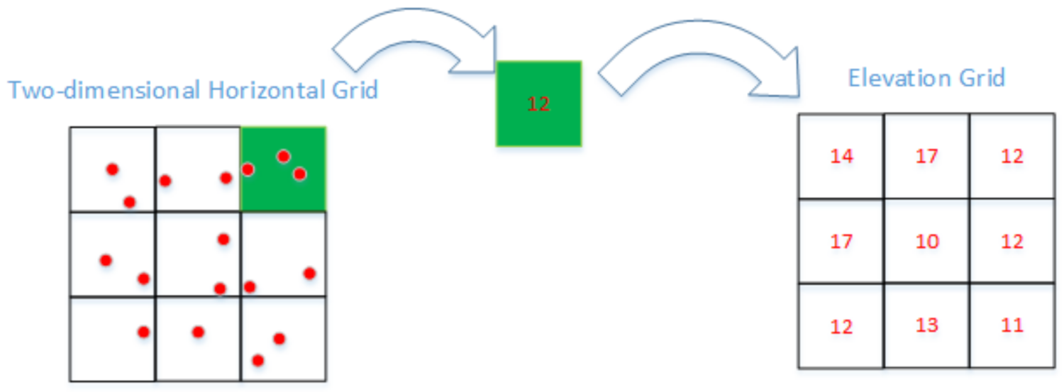
2.1. Data Preprocessing
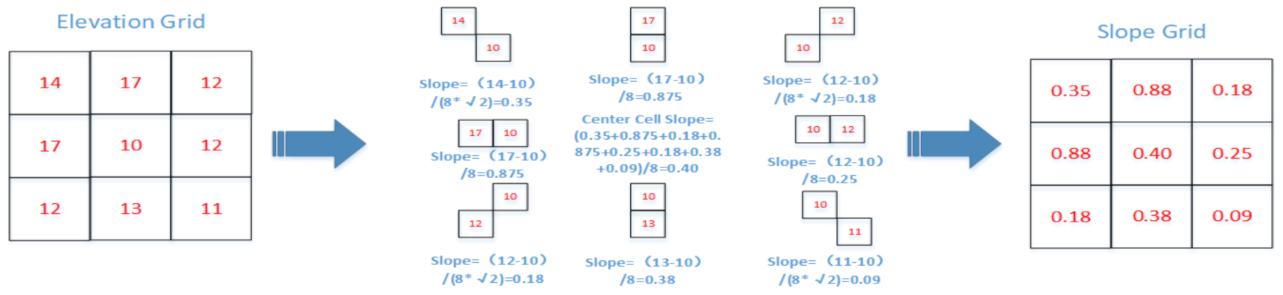
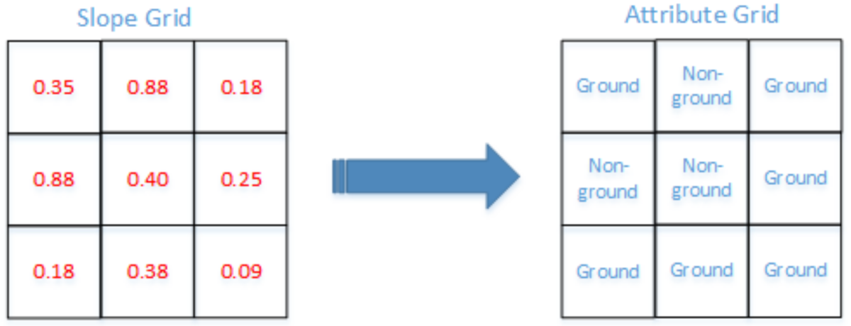
2.2. The Slope Filter


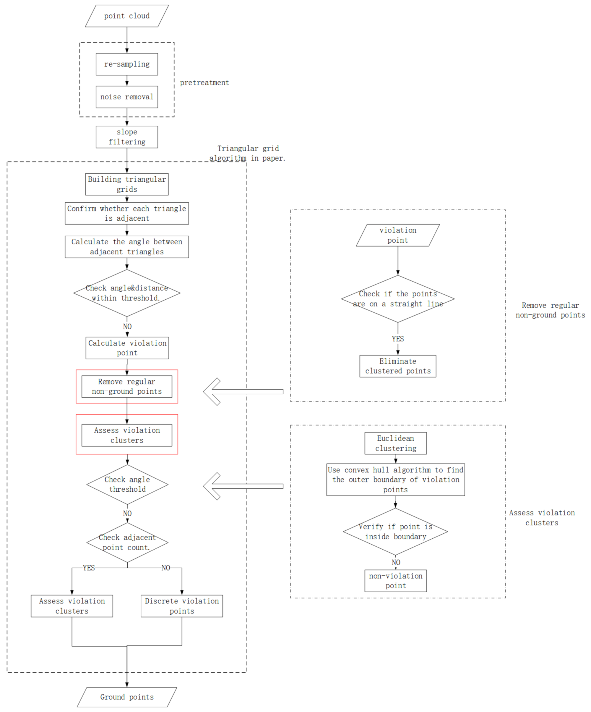
2.3. Constructing a Triangular Grid and Identifying Violation Points
- (1)
- Calculate the normal vector of adjacent triangles in sequence by the calibration number of triangles (, Equation (2)), then substitute the coordinates into (2) to determine the surface normal vector (, Equation (3));
- (2)
- Determine that the angle between the two planes is equal to the angle between the normal vectors of the two planes to obtain the angle between the two triangles (, Equation (4));
- (3)
- Estimate the angle and longest side length of each triangle with a threshold, and if they are more than the threshold range, the selection of a threshold angle and side length of 70° and 4 m, respectively, allows the extraction of most of the scene violation points; mark these triangles as violation triangles. Continue until all triangles are judged;
- (4)
- Extract the maximum value of each violation triangle as violation points.

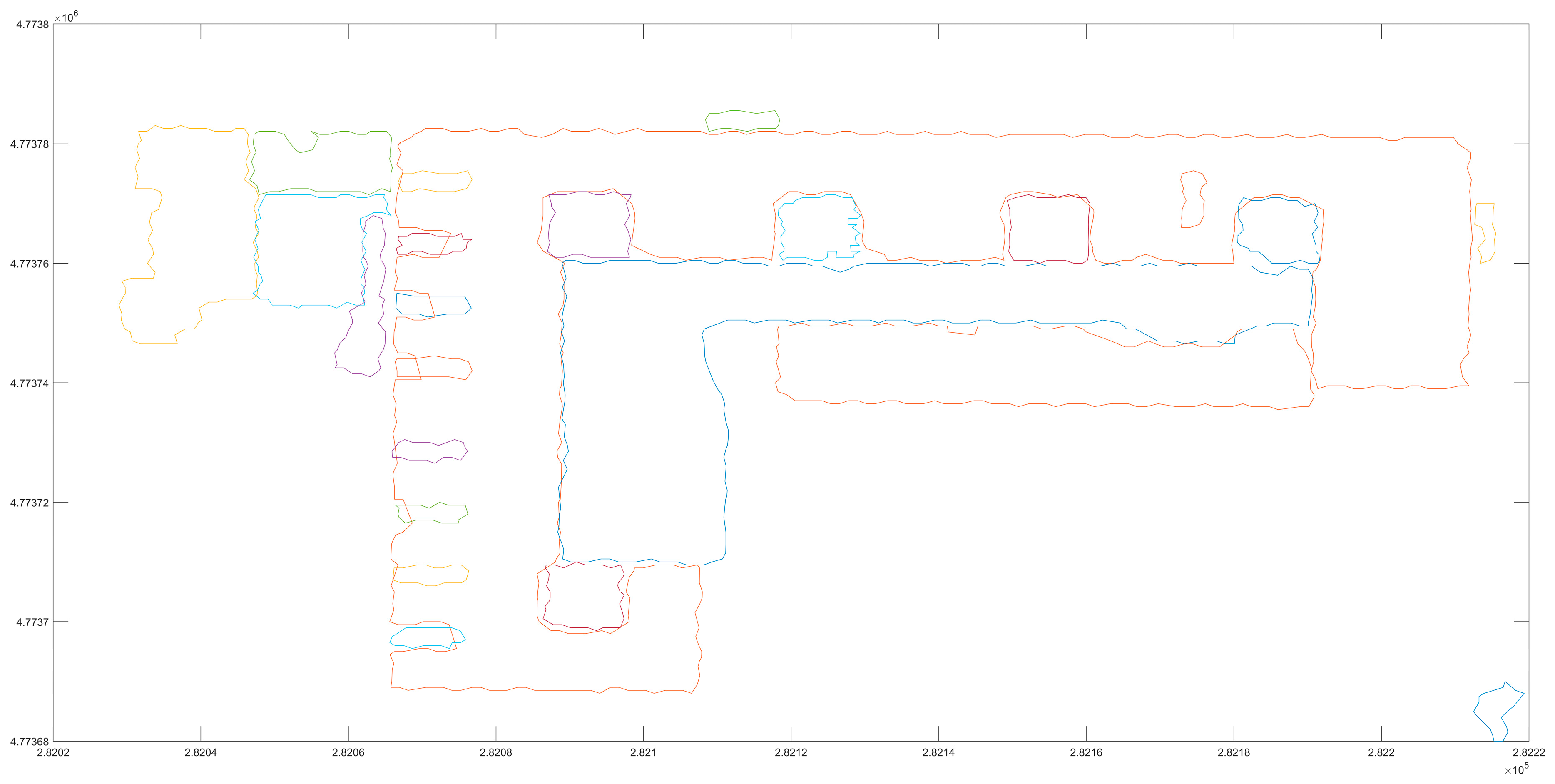
2.4. Collinear Judgment
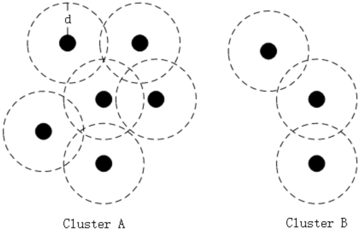
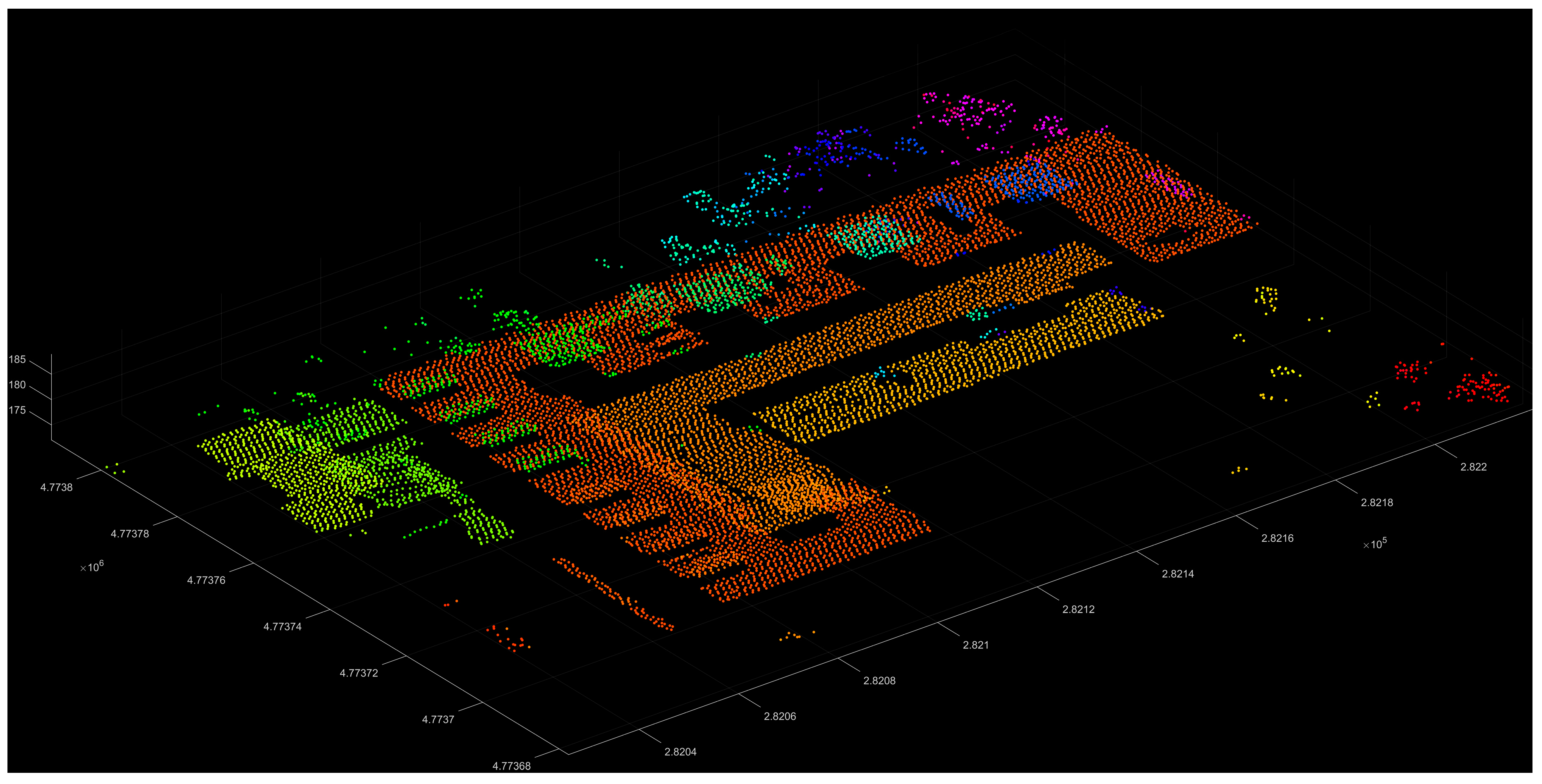
2.5. Cluster Point Classification
- (1)
- Select a point from the regular violation point set, T, which is assessed by the collinear judgment as the cluster center point;
- (2)
- Perform a neighbor point index based on the KD-Tree using the original point cloud data;
- (3)
- Find the points within the distance threshold and add these points to the undetermined set P;
- (4)
- Check whether the number of points in p increases or if the height difference is overrun; in which case, repeat steps 2–3 until the number of points in P does not increase;
- (5)
- Output the P set and remove P from Q;
- (6)
- Remove the points that are repeated with P from T to avoid repeated operations, which increase the amount of calculation;
- (7)
- Check whether all the points in T have been calculated, and repeat steps 2–6 until there are no unoperated points.


3. The Experimental Procedure
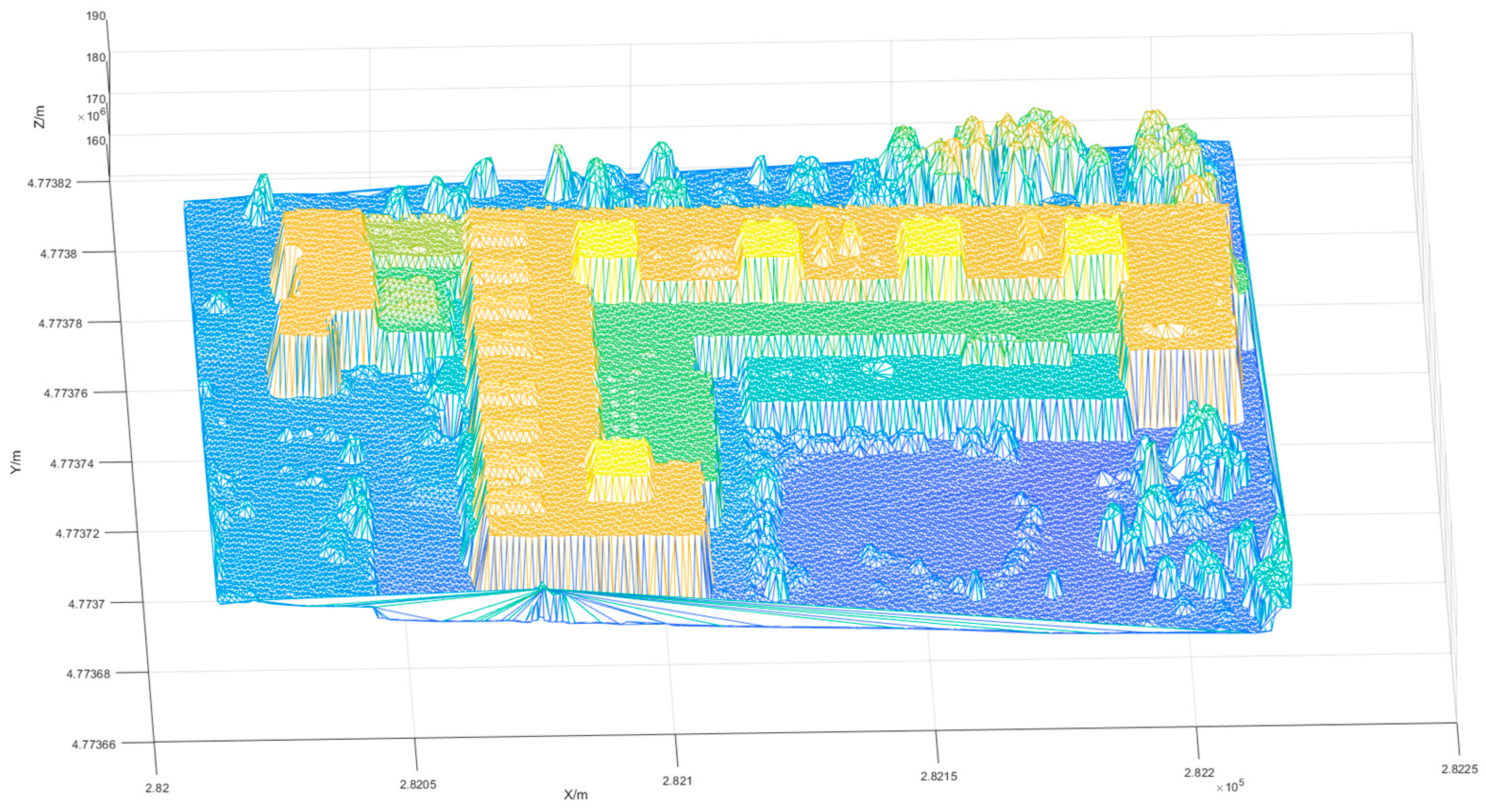
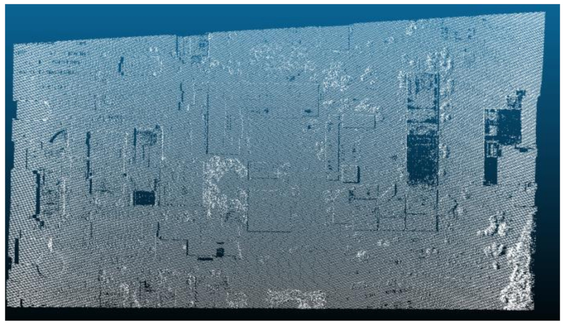
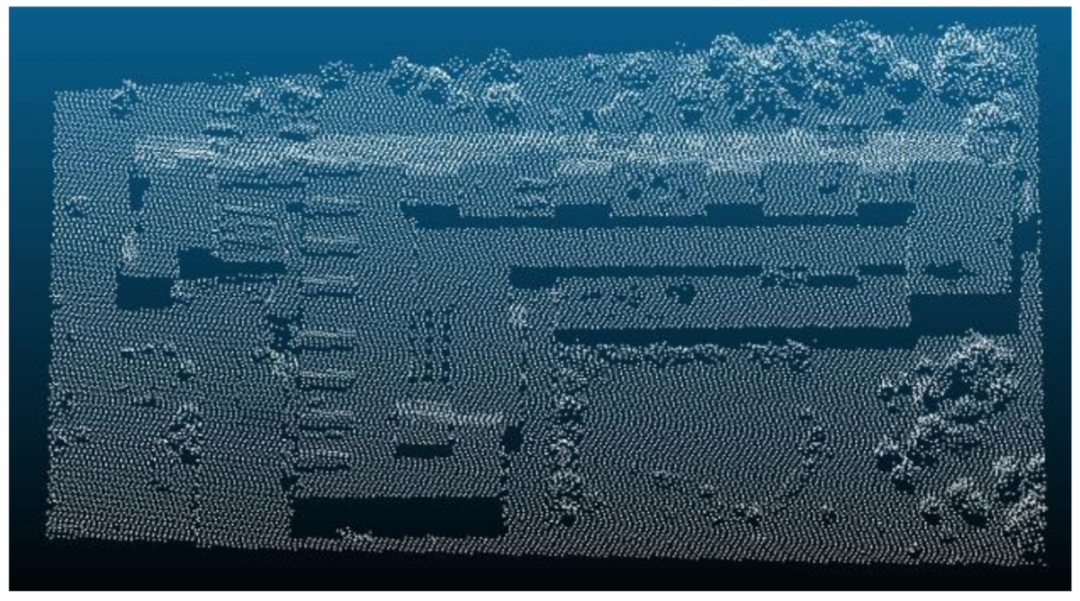
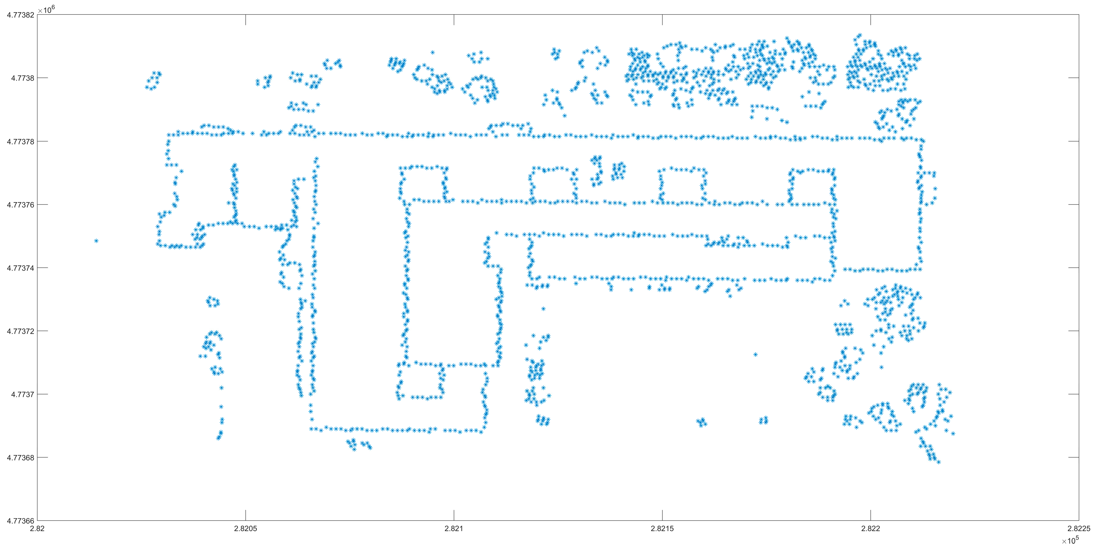
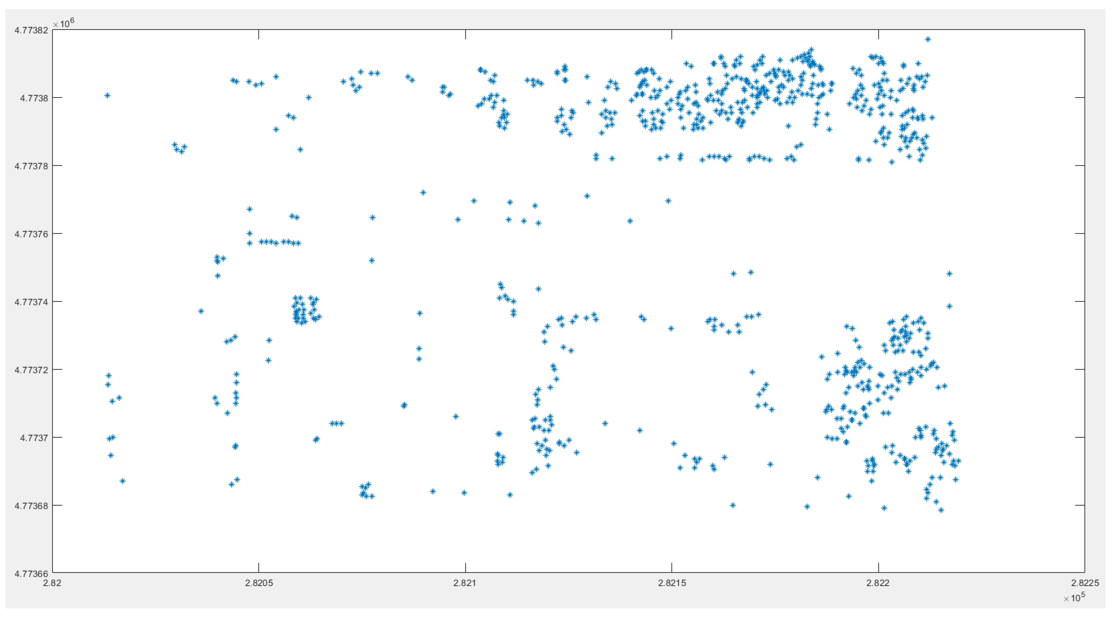
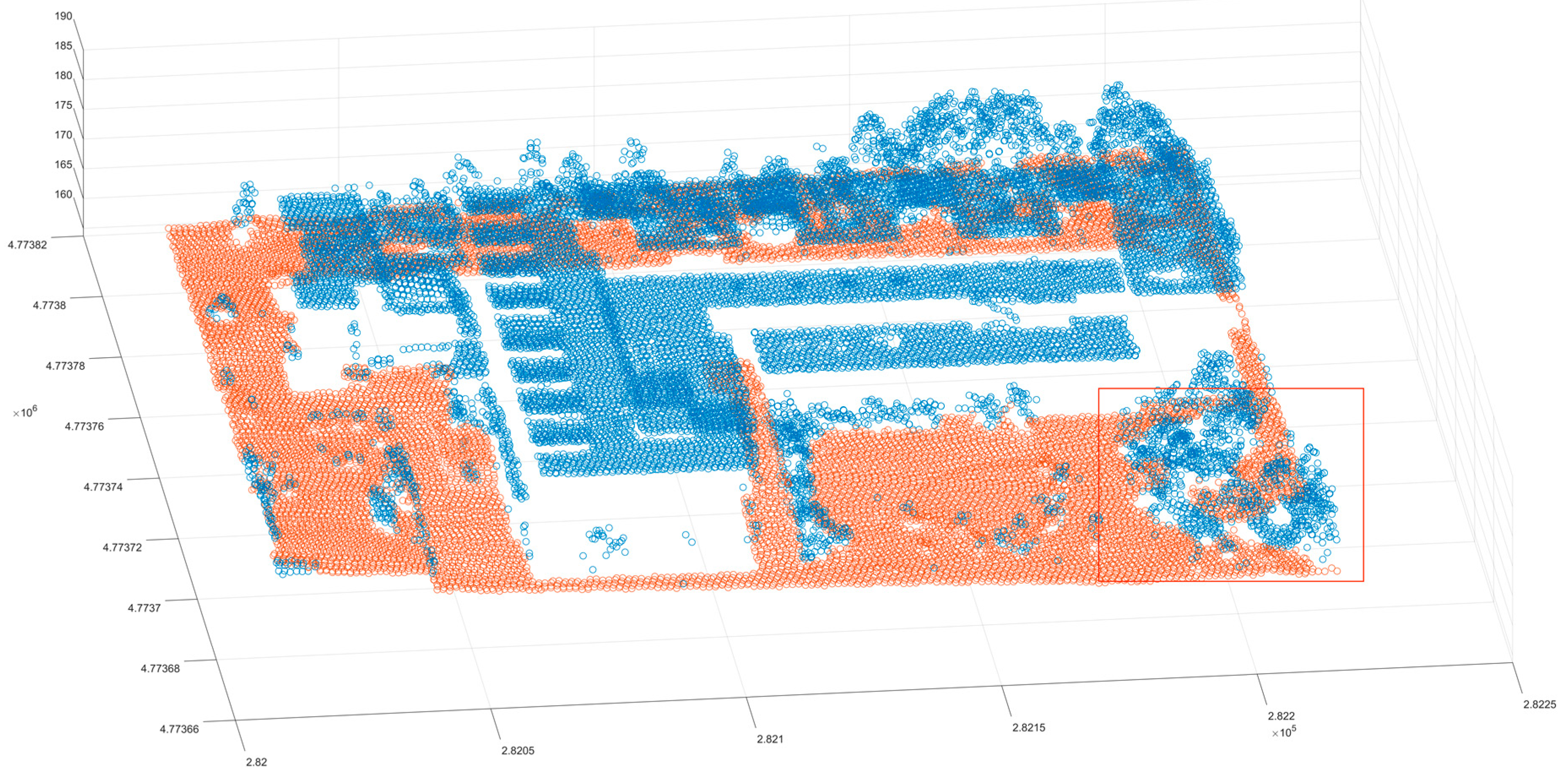
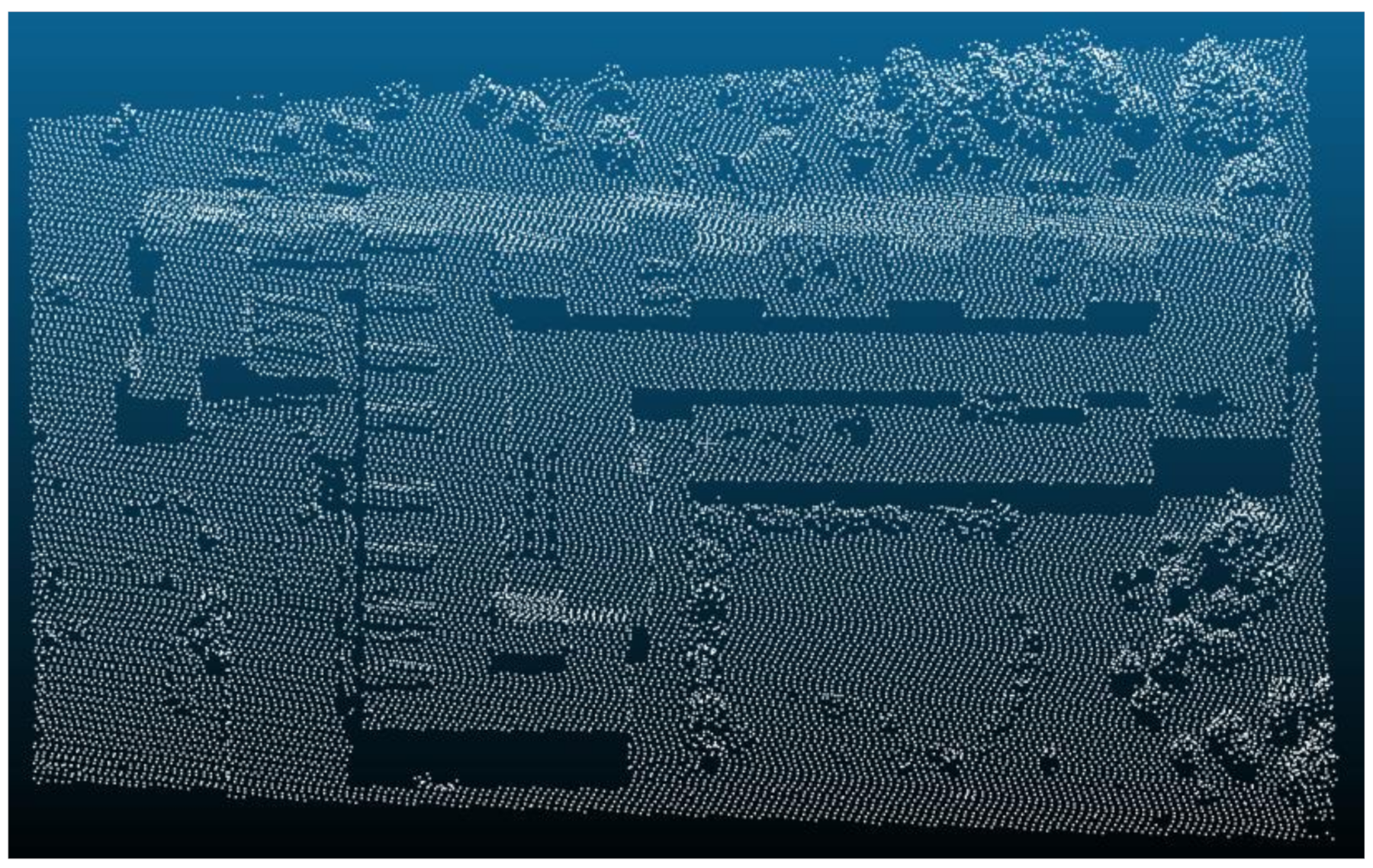
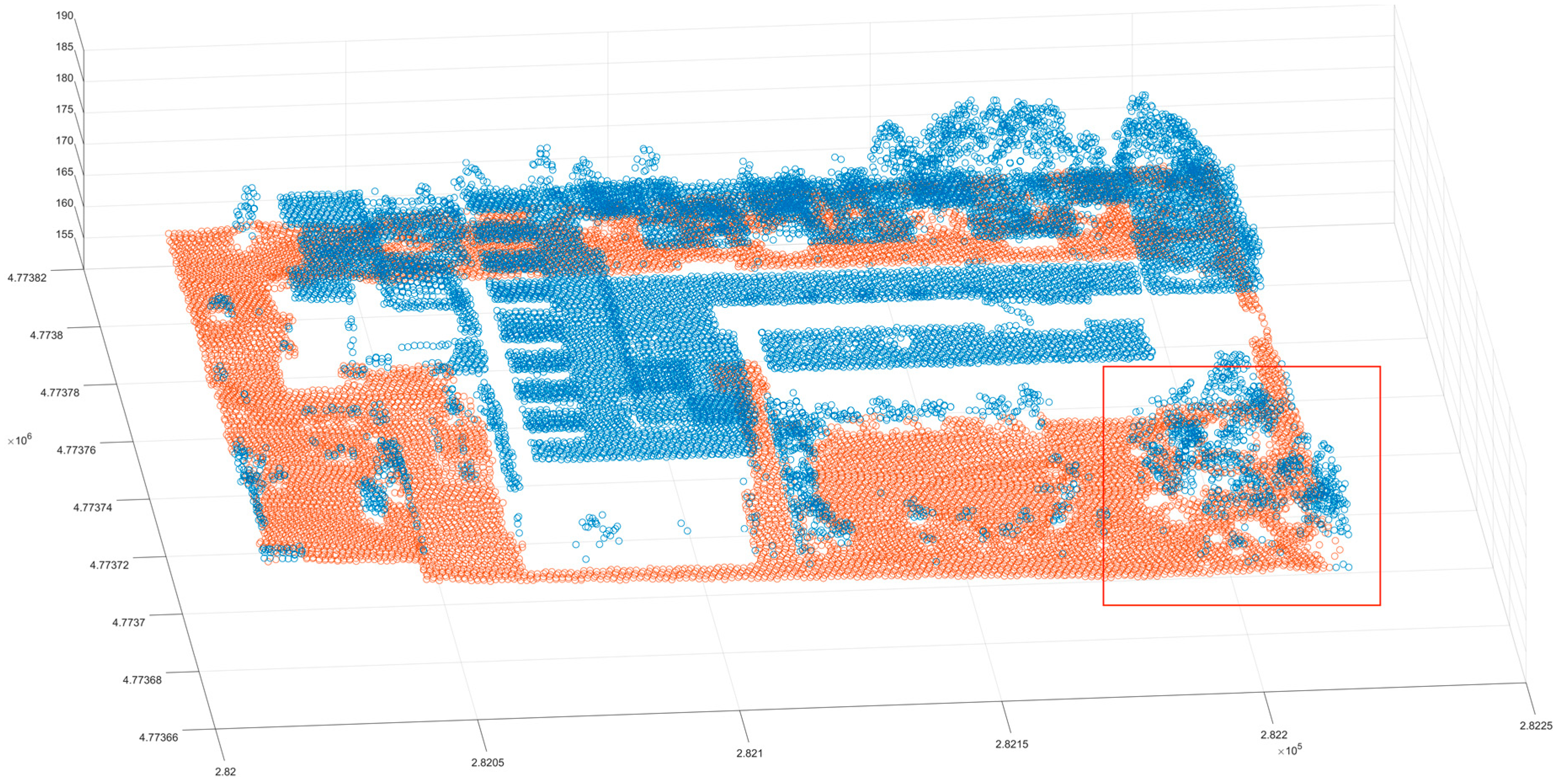
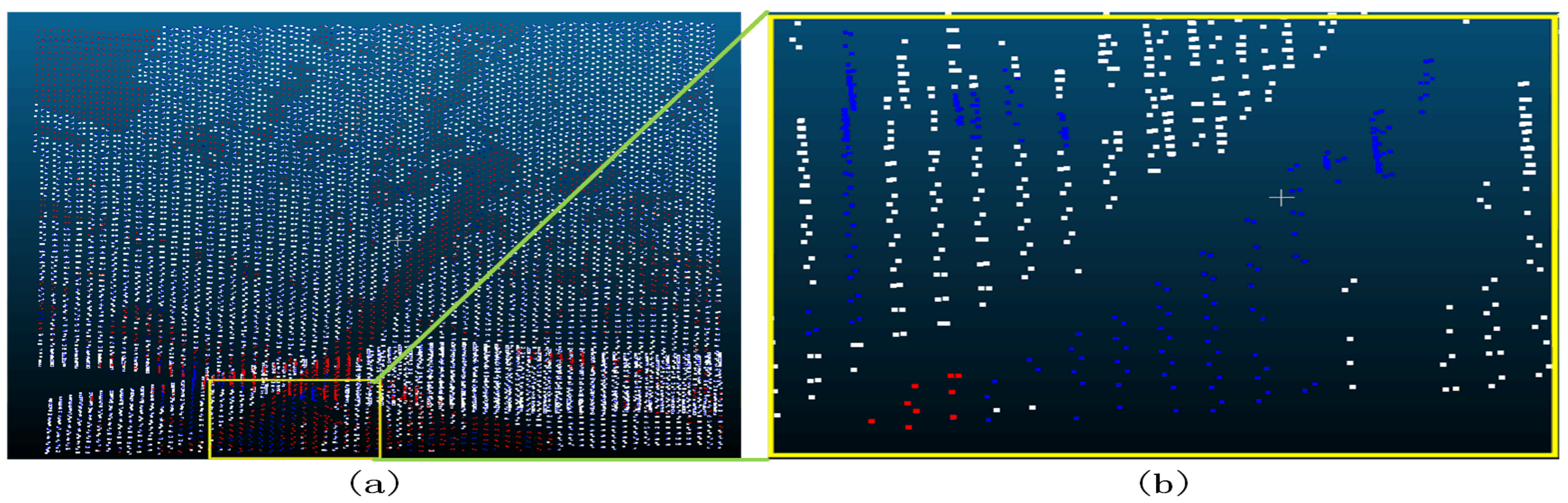
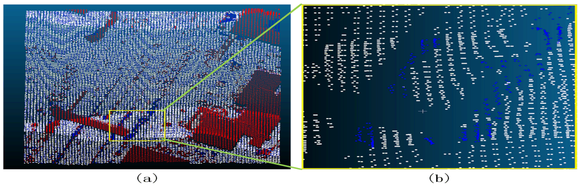
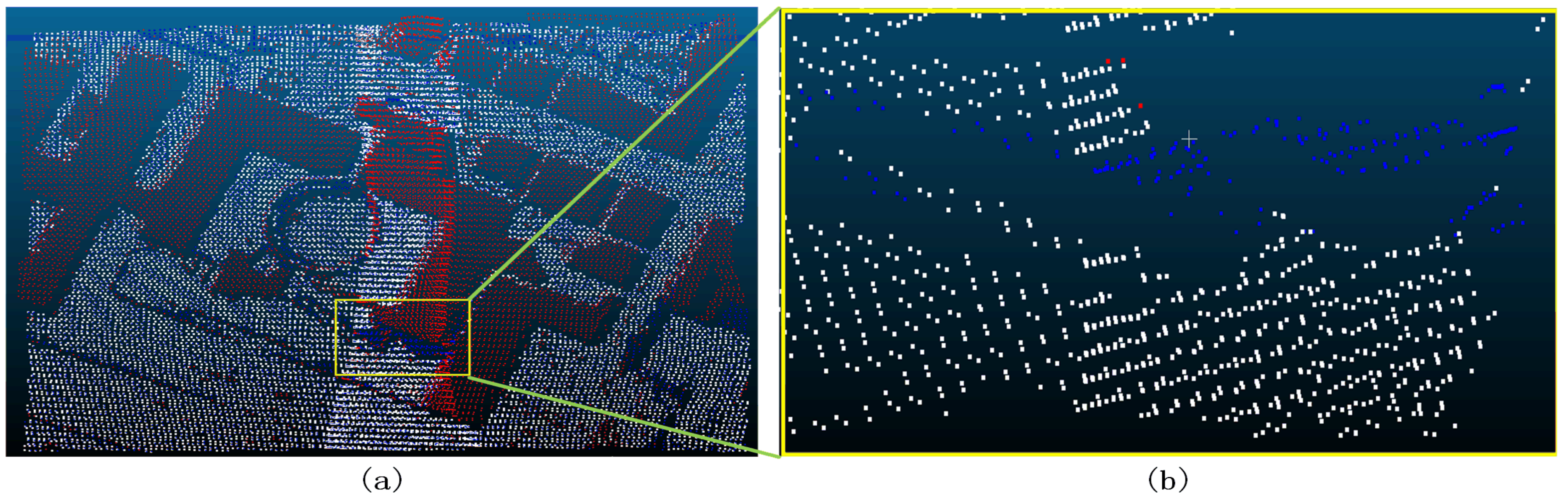
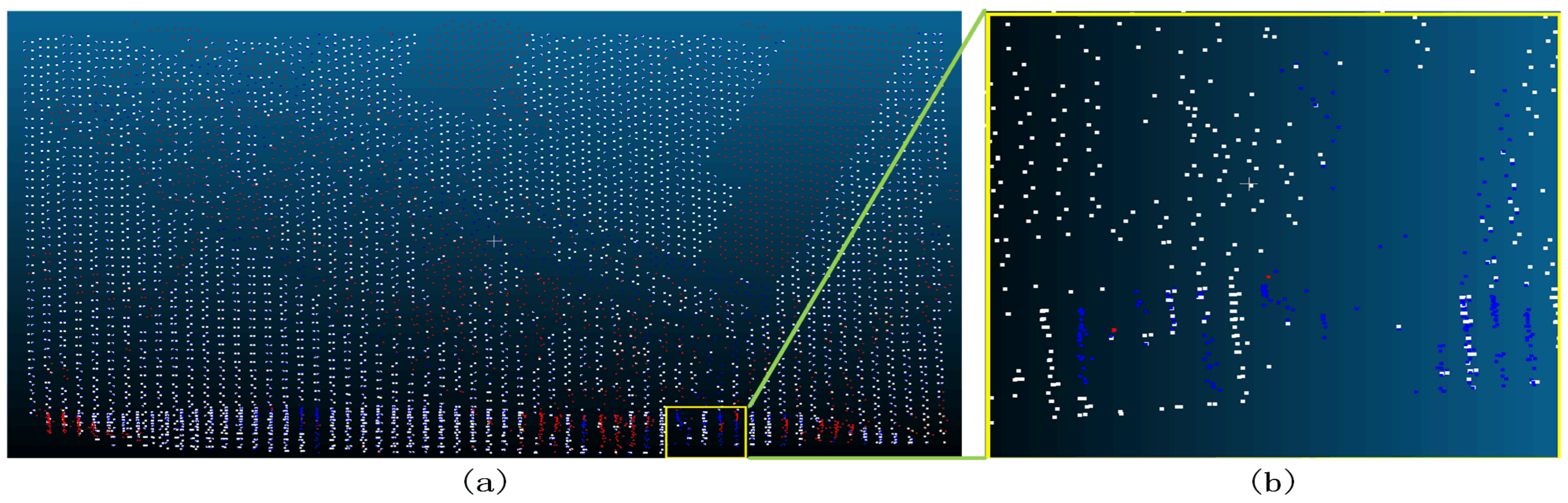
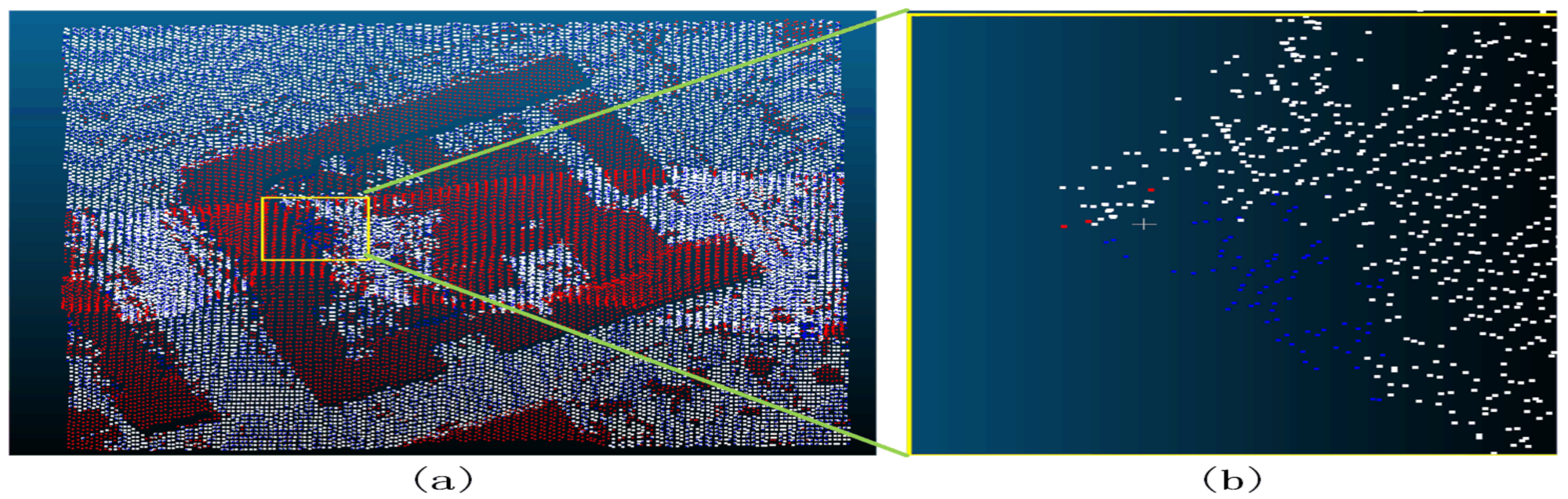
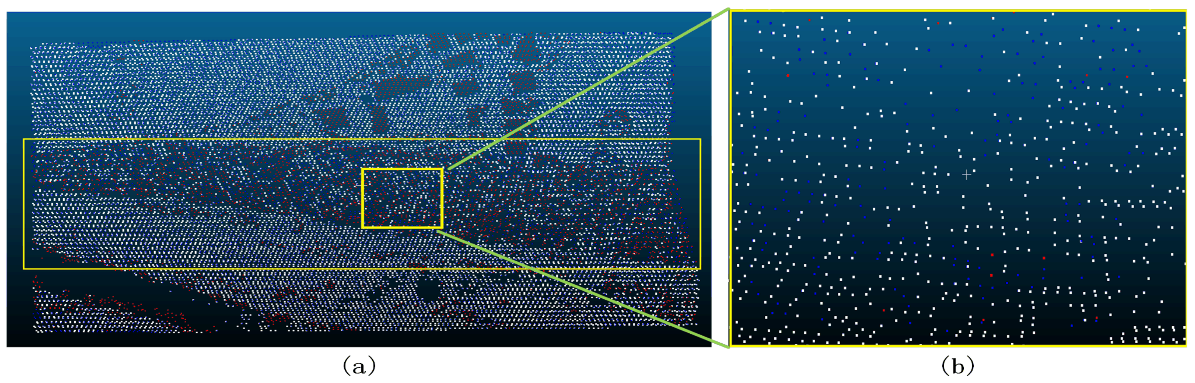
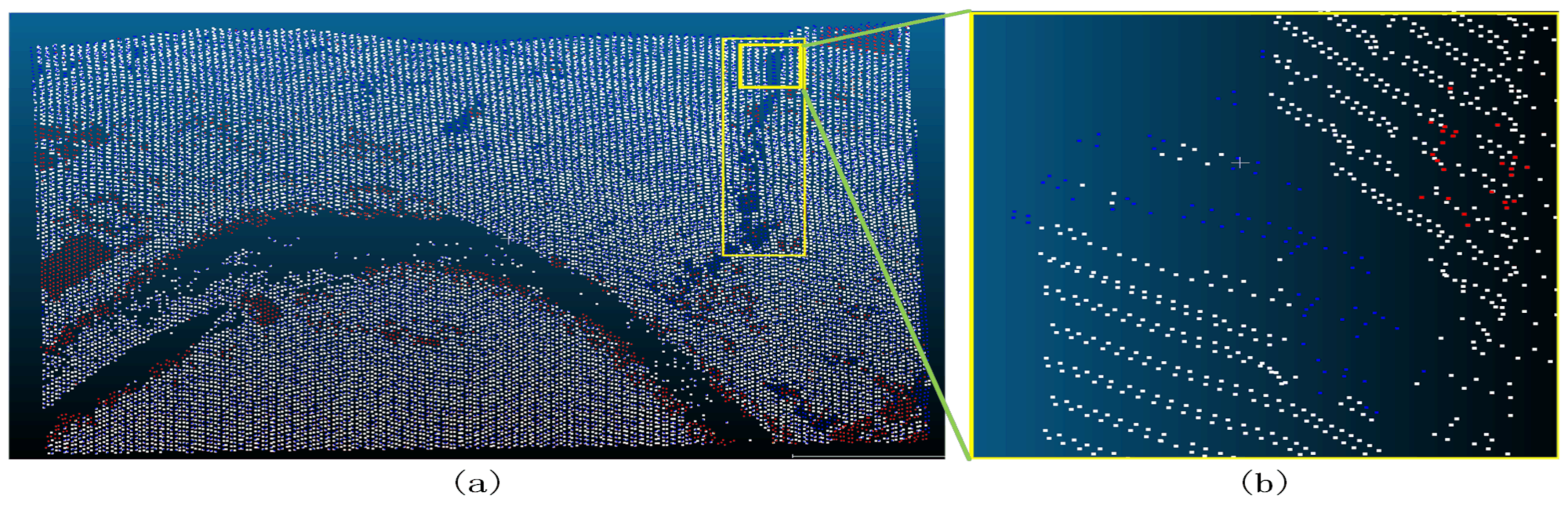
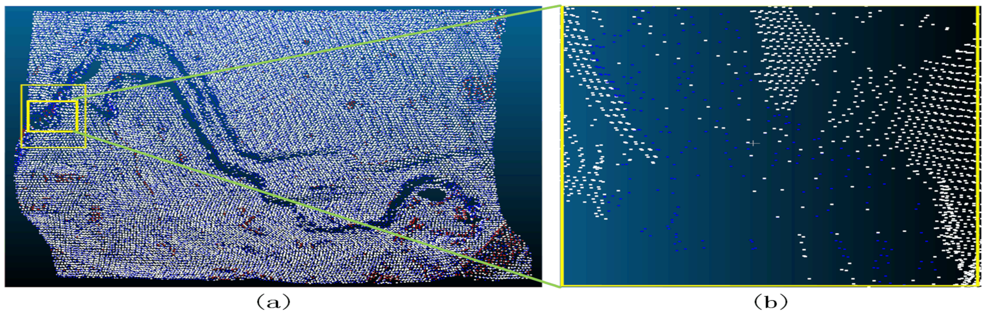
3.1. Experimental Data and Evaluation Criteria
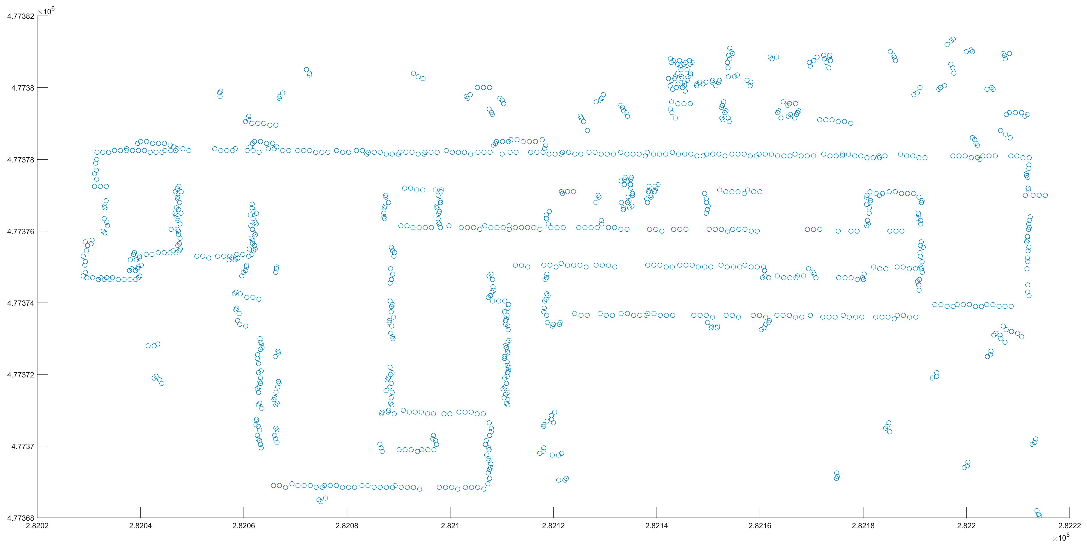
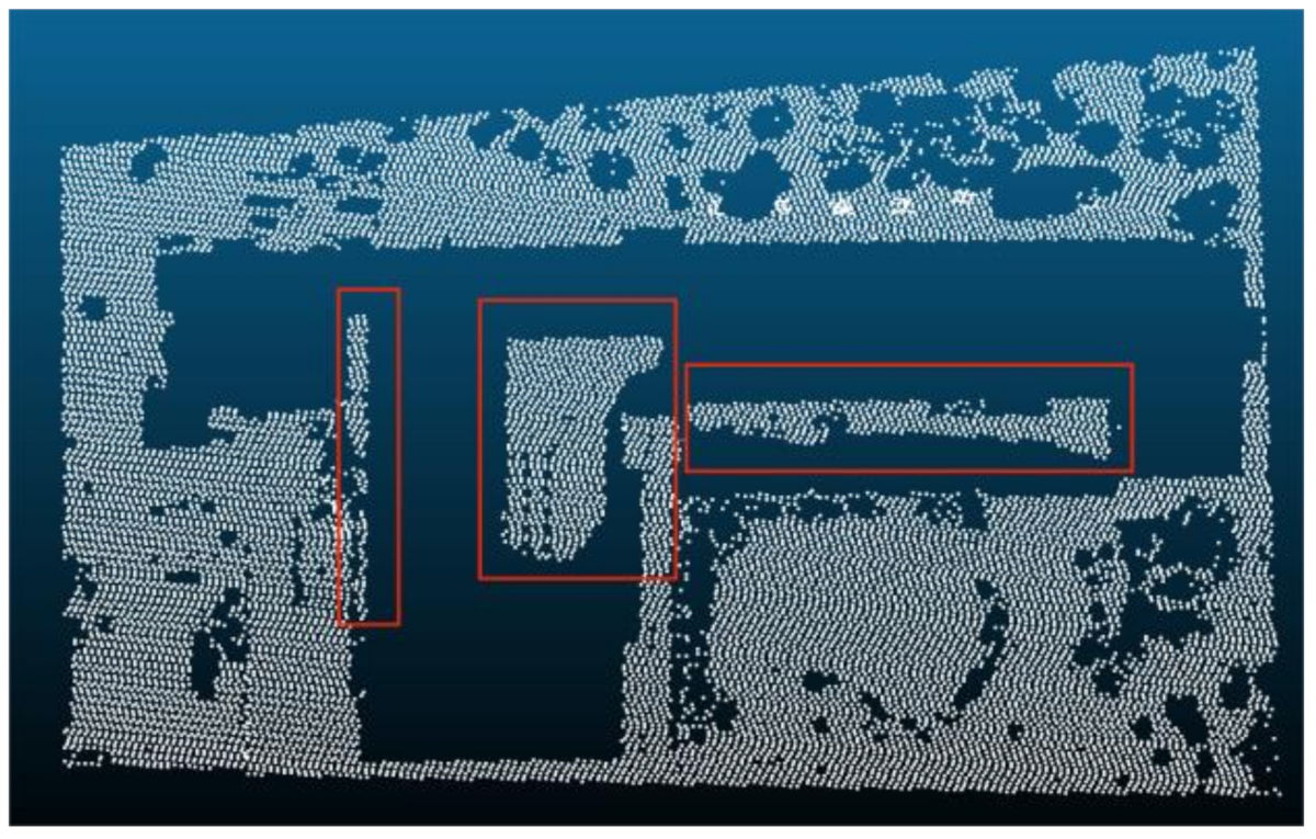
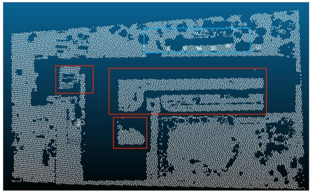
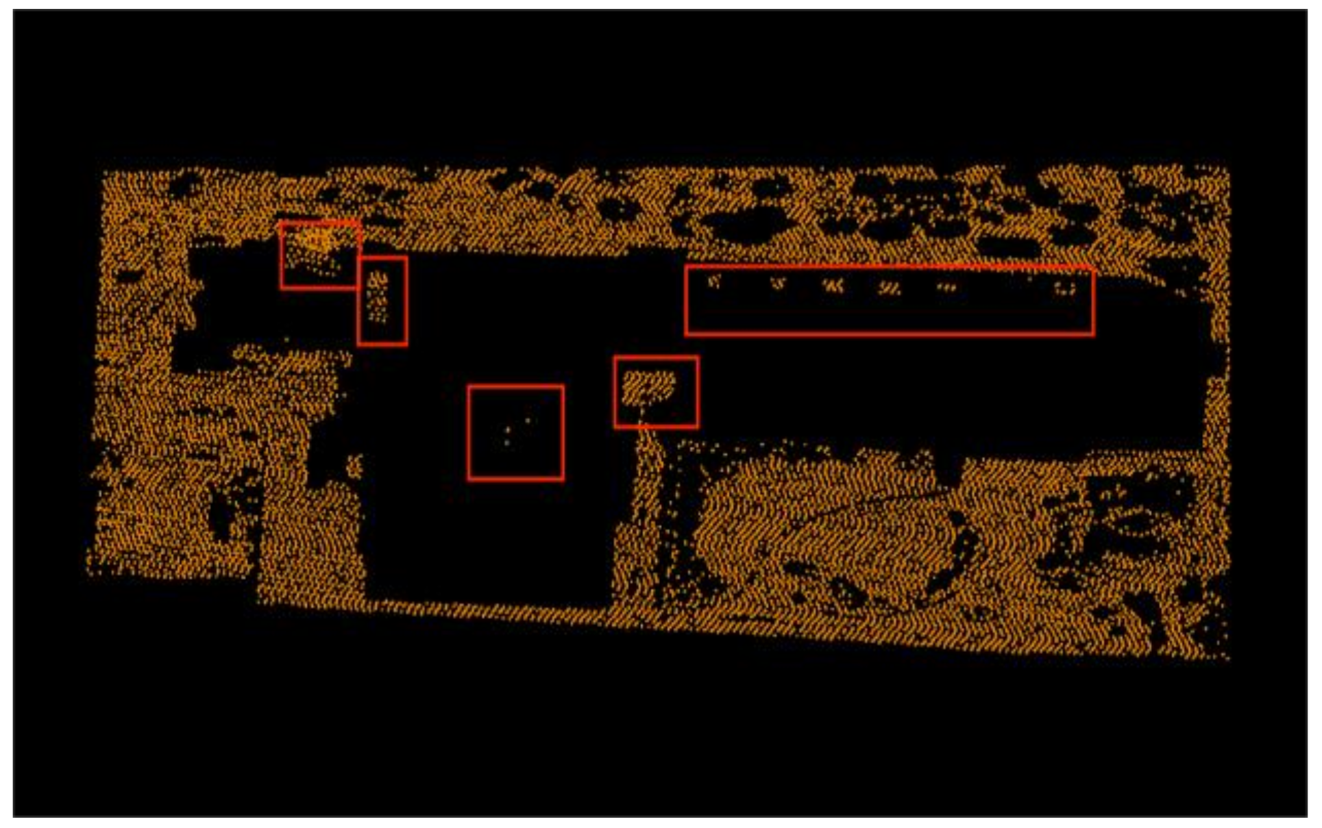
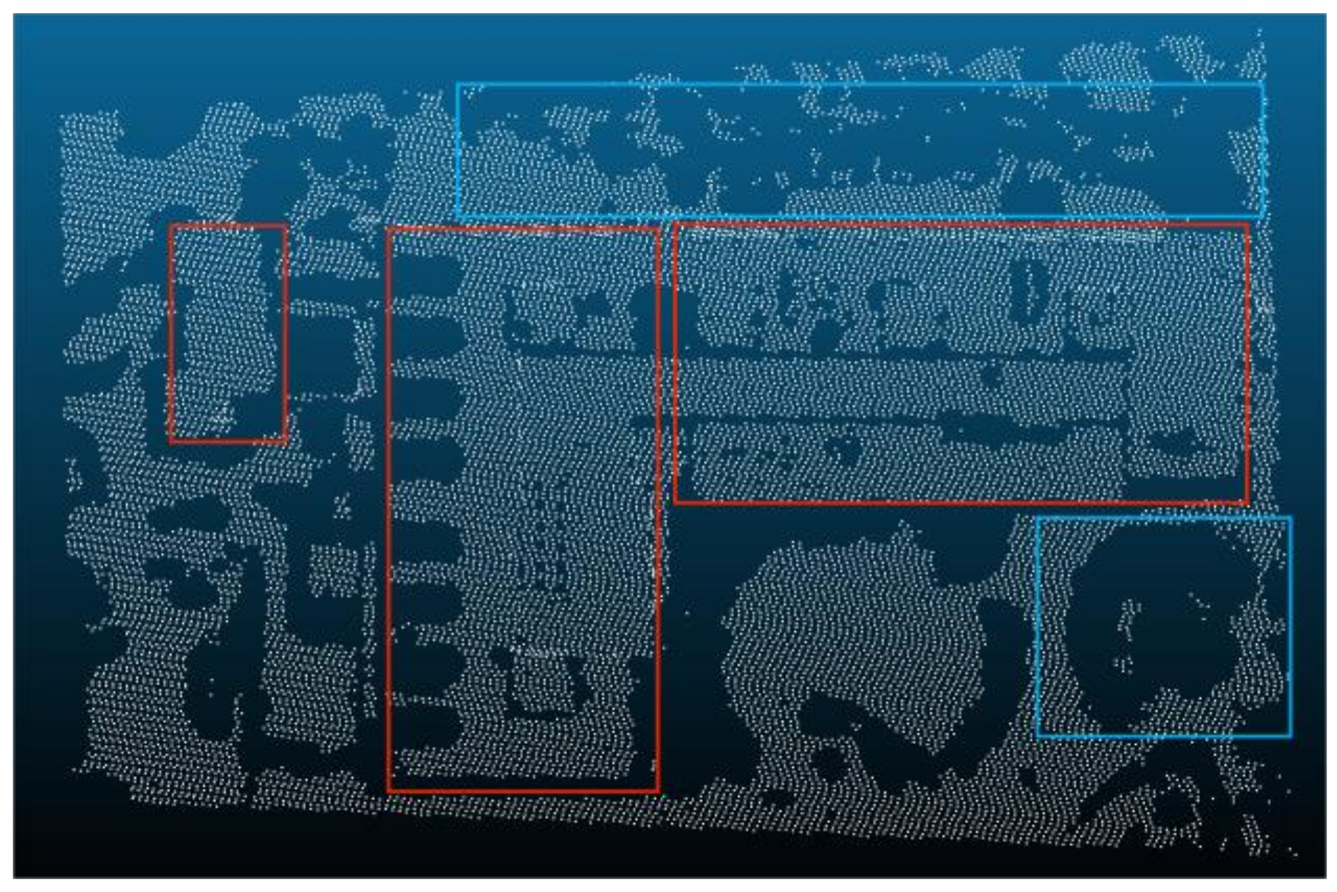
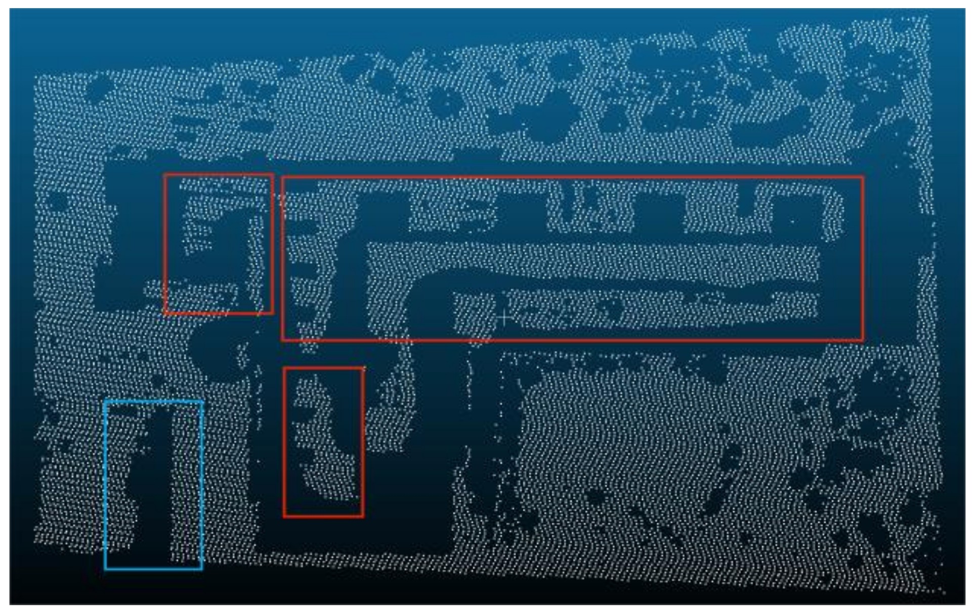
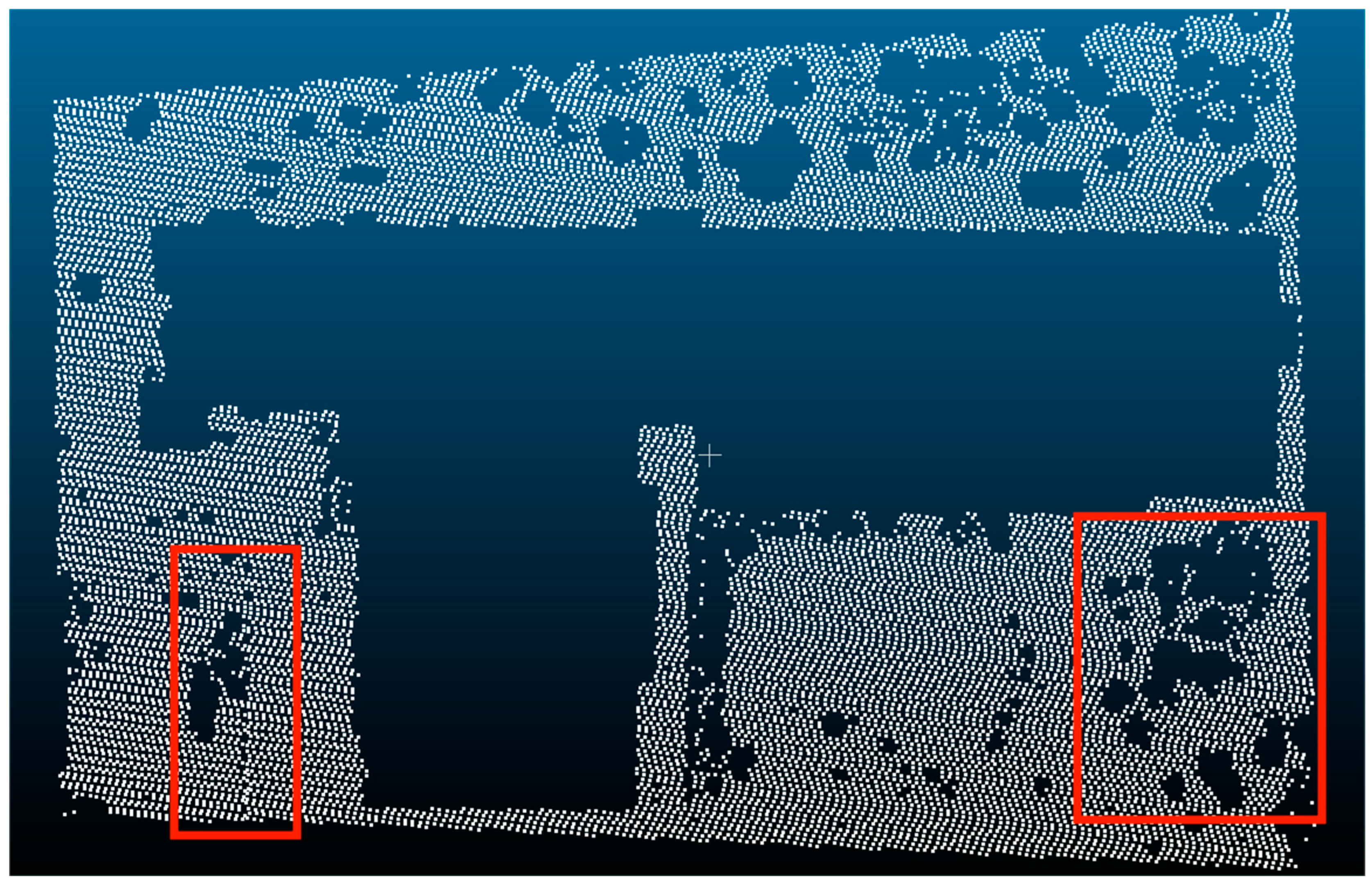
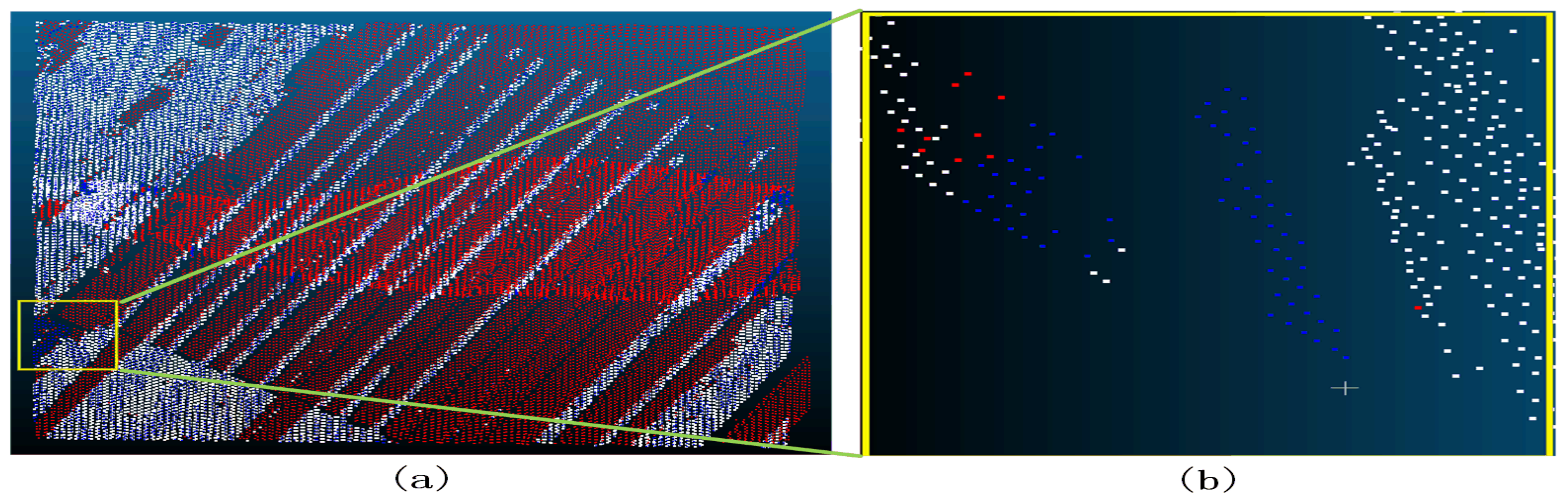
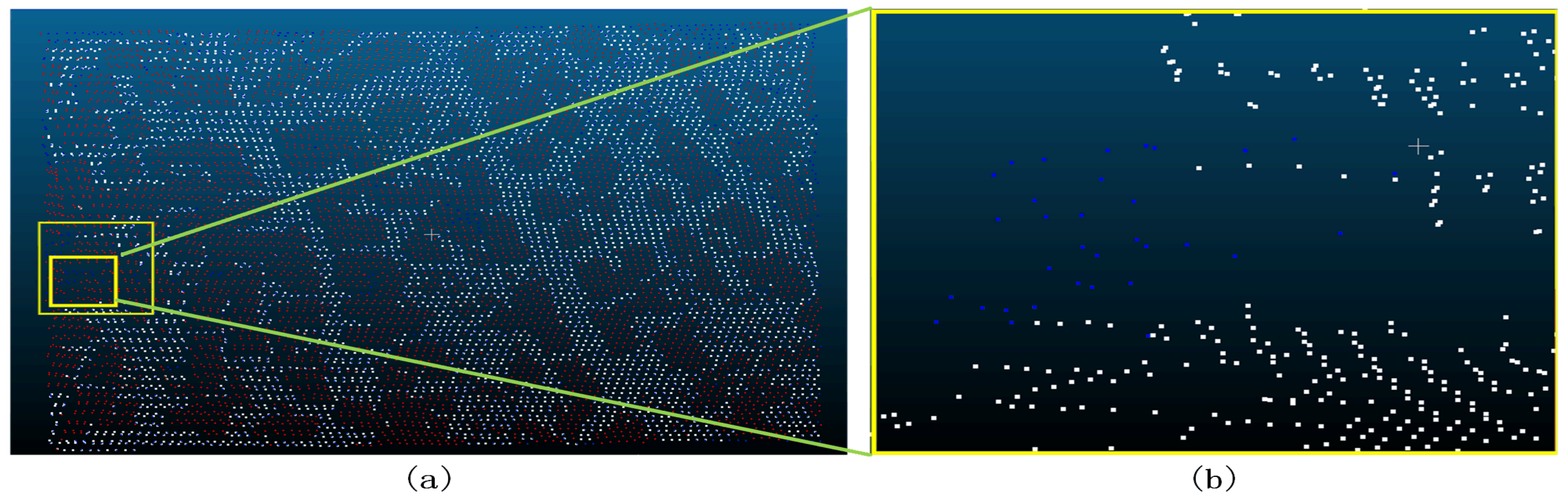
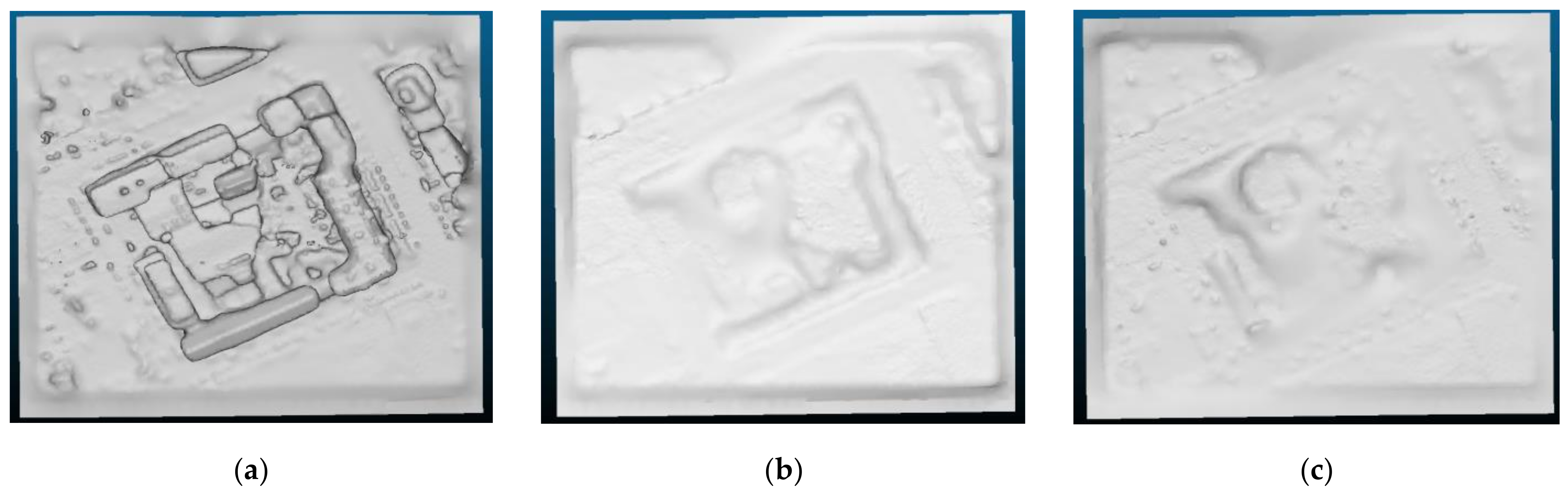
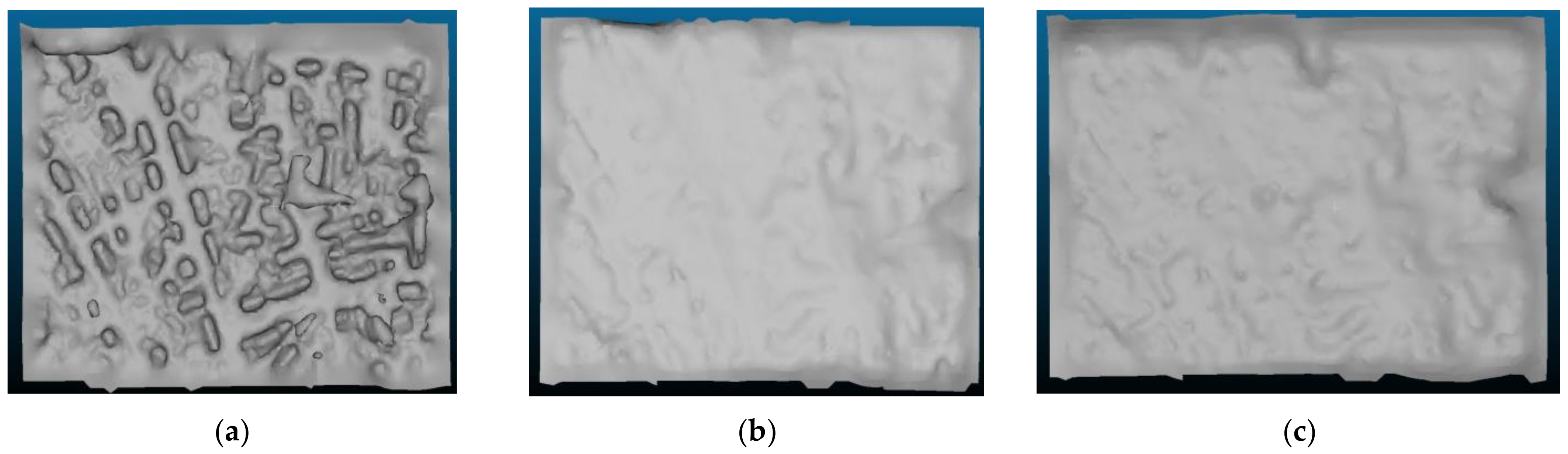
3.2. The Process of the Triangulation Method Filter
- (1)
- When there are several separate points in the same area and the distance between them is also within the distance threshold, this situation needs to be removed because it will be easy to remove the ground points between these separate points;
- (2)
- The points in the group may be due to the collinear situation of some forest points because the forest is roughly uneven, and this is why an elevation value is set. These groups may be composed of forest points that are misjudged as regular violation points and have forest points in close proximity.


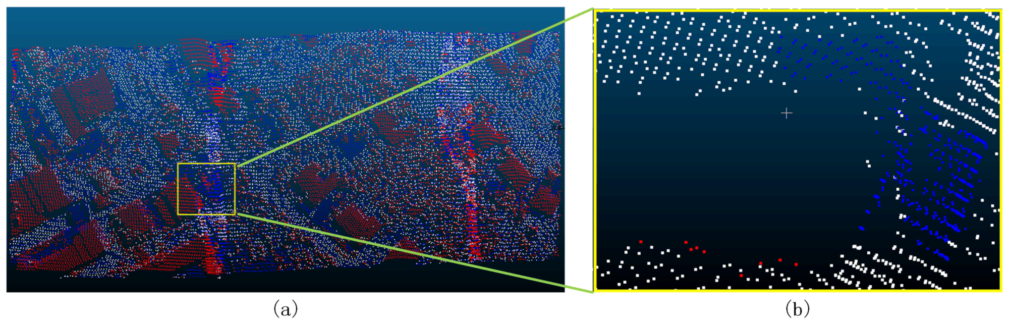
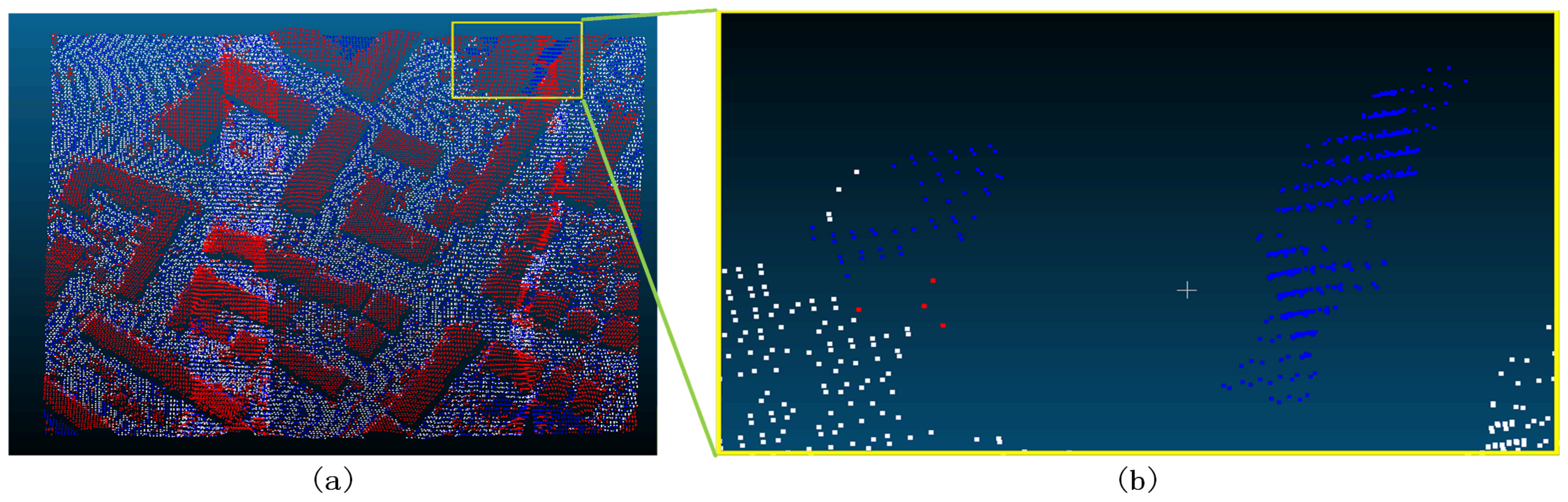
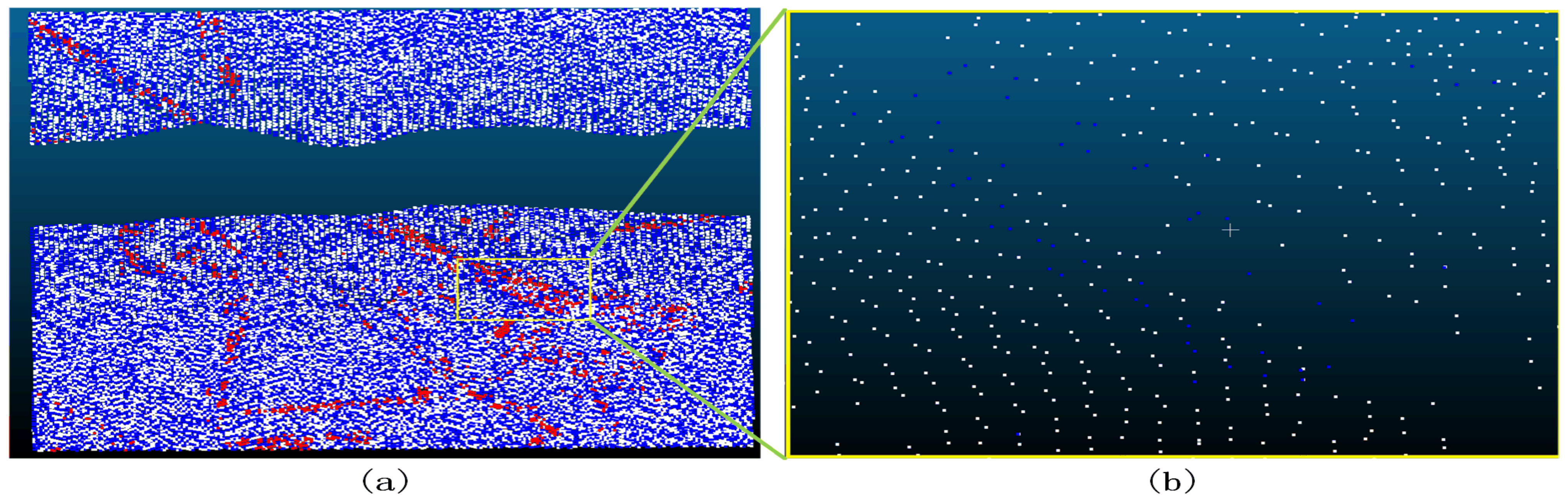
3.3. Data Comparison
4. Discussion
- (1)
- The clustering algorithm is still not perfect, as it fails to adjust the distance threshold based on the point cloud distribution in the relevant scene being studied;
- (2)
- This method needs to construct a triangular grid for each point in the point cloud, so the processing speed of point cloud data with large scenes is relatively slow, and complex scenes require repeated operations;
- (3)
- The filter effect is poor when the slope on discontinuous ground changes significantly.
5. Conclusions
- (1)
- The clustering algorithm used a fixed threshold when obtaining non-ground points; however, it is easy to misclassify ground points that are closer to non-ground points. Our future research proposes a clustering method that can adopt an adaptive threshold;
- (2)
- After each round of point cloud filtering, it is necessary to rebuild the grid, which reduces the efficiency of some operations. Our future research proposes the gradual optimization of the present algorithm model to further enhance its computational efficiency;
- (3)
- For scenes with more scatter distribution, the filtering effect may be poor. In the future, we will further optimize the scatter scene model to enhance the accuracy of the operation.
Author Contributions
Funding
Data Availability Statement
Acknowledgments
Conflicts of Interest
Abbreviations
| ISPRS | International Society for Photogrammetry and Remote Sensing |
| EMD | Empirical Mode Decomposition |
| SMRF | Simple Morphological Filter |
References
- Lv, D.; Ying, X.; Cui, Y.; Song, J.; Qian, K.; Li, M. Research on the technology of LIDAR data processing. In Proceedings of the 2017 First International Conference on Electronics Instrumentation & Information Systems (EIIS), Harbin, China, 3–5 June 2017; IEEE: Piscataway, NJ, USA, 2017; pp. 1–5. [Google Scholar]
- Sithole, G.; Vosselman, G. Comparison of filtering algorithms. In Proceedings of the ISPRS working group III/3 workshop, Dresden, Germany, 8–10 October 2003; pp. 71–78. [Google Scholar]
- Zheng, Z.; Jingui, Z.; Haiyang, H. Comparative analysis of different airborne LiDAR point cloud filtering algorithms. Surv. Geogr. Inf. 2021, 46, 52–56. [Google Scholar] [CrossRef]
- Huang, H.; Su, P.; Wang, R.; Wang, F.; Shi, W.; Zhao, J. The feasibility study of DEM production based on dense matching point cloud. Bull. Surv. Mapp. 2022, 170, 170–174. [Google Scholar] [CrossRef]
- Lin, X.; Zhang, J. Segmentation-based filtering of airborne LiDAR point clouds by progressive densification of terrain segments. Remote Sens. 2014, 6, 1294–1326. [Google Scholar] [CrossRef] [Green Version]
- Zhang, W.; Qi, J.; Wan, P.; Wang, H.; Xie, D.; Wang, X. An easy-to-use airborne LiDAR data Filter method based on cloth simulation. Remote Sens. 2016, 8, 501. [Google Scholar] [CrossRef]
- Vosselman, G. Slope based Filter of laser altimetry data. Int. Arch. Photogramm. Remote Sens. 2000, 33, 935–942. [Google Scholar]
- Zhu, X.; Wang, C.; Xi, X.; Wang, P.; Tian, X.; Yang, X. Adaptive threshold point cloud Filter method for multi-level moving surface fitting. J. Surv. Mapp. 2018, 47, 153–160. [Google Scholar]
- Wang, W.; Li, Z.; Fu, Y.; He, H.; Xiong, F. A Multi-scale Adaptive Slope Filter Algorithm for Point Cloud. J. Wuhan Univ. 2022, 47, 438–446. [Google Scholar]
- Shahzad, M.; Zhu, X.X. Reconstructing 2-D/3-D building shapes from spaceborne tomographic SAR point clouds. ISPRS 2014, 40, 313–320. [Google Scholar]
- Zhu, X.X.; Shahzad, M. Facade reconstruction using multiview spaceborne TomoSAR point clouds. IEEE Trans. Geosci. Remote Sens. 2013, 52, 3541–3552. [Google Scholar] [CrossRef]
- Guo, Z.; Liu, H.; Shi, H.; Li, F.; Guo, X.; Cheng, B. KD-Tree-Based Euclidean Clustering for Tomographic SAR Point Cloud Extraction and Segmentation. IEEE Geosci. Remote Sens. Lett. 2023, 20, 4000205. [Google Scholar] [CrossRef]
- Rodriguez, A.; Laio, A. Clustering by fast search and find of density peaks. Science 2014, 344, 1492–1496. [Google Scholar] [CrossRef] [PubMed] [Green Version]
- Chen, X.; Wu, H.; Lichti, D.; Han, X.; Ban, Y.; Li, P.; Deng, H. Extraction of indoor objects based on the exponential function density clustering model. Inf. Sci. 2022, 607, 1111–1135. [Google Scholar] [CrossRef]
- Sun, S.; Salvaggio, C. Aerial 3D building detection and modeling from airborne LiDAR point clouds. IEEE J. Sel. Top. Appl. Earth Obs. Remote Sens. 2013, 6, 1440–1449. [Google Scholar]
- Gamal, A.; Wibisono, A.; Wicaksono, S.B.; Abyan, M.A.; Hamid, N.; Wisesa, H.A.; Jatmiko, W.; Ardhianto, R. Automatic LIDAR building segmentation based on DGCNN and euclidean clustering. J. Big Data 2020, 7, 102. [Google Scholar] [CrossRef]
- Xu, Z.; Kang, R.; Lu, R. 3D reconstruction and measurement of surface defects in prefabricated elements using point clouds. J. Comput. Civ. Eng. 2020, 34, 04020033. [Google Scholar] [CrossRef]
- Caumon, G.; Collon-Drouaillet, P.; Le Carlier de Veslud, C.; Viseur, S.; Sausse, J. Surface-based 3D modeling of geological structures. Math. Geosci. 2009, 41, 927–945. [Google Scholar]
- Greene, E.; Frawley, W.; Swimm, R. Individual differences in collinearity judgment as a function of angular position. Percept. Psychophys. 2000, 62, 1440–1458. [Google Scholar] [CrossRef]
- Huang, J.; Stoter, J.; Peters, R.; Nan, L. City3D: Large-scale building reconstruction from airborne LiDAR point clouds. Remote Sens. 2022, 14, 2254. [Google Scholar] [CrossRef]
- Albano, R. Investigation on roof segmentation for 3D building reconstruction from aerial LIDAR point clouds. Appl. Sci. 2019, 9, 4674. [Google Scholar]
- Huang, N.E. Review of empirical mode decomposition. In Proceedings of the Aerospace/Defense Sensing, Simulation, and Controls, Orlando, FL, USA, 26 March 2001; Wavelet Applications VIII SPIE 4391. pp. 71–80. [Google Scholar]
- Pingel, T.J.; Clarke, K.C.; McBride, W.A. An improved simple morphological filter for the terrain classification of airborne LIDAR data. ISPRS J. Photogramm. Remote Sens. 2013, 77, 21–30. [Google Scholar] [CrossRef]
- Pfeifer, N.; Reiter, T.; Briese, C.; Rieger, W. Interpolation of high quality ground models from laser scanner data in forested areas. Int. Arch. Photogramm. Remote Sens. 1999, 32, 31–36. [Google Scholar]
- Sohn, G.; Dowman, I.J. Terrain surface reconstruction by the use of tetrahedron model with the MDL criterion. In International Archives of Photogrammetry Remote Sensing and Spatial Information Sciences; Natural Resources Canada: Ottawa, ON, Canada, 2002; Volume 34, pp. 336–344. [Google Scholar]
- Elmqvist, M. Automatic Ground Modeling Using Laser Radar Data. Master’s Thesis, Linkoping University, Linköping, Sweden, 2000. [Google Scholar]
- Roggero, M. Airborne laser scanning-clustering in raw data. Int. Arch. Photogramm. Remote Sens. Spat. Inf. Sci. 2001, 34, 227–232. [Google Scholar]
- Brovelli, M.A.; Cannata, M.; Longoni, U.M. Managing and processing LIDAR data within GRASS. In Proceedings of the Open source GIS—GRASS Users Conference 2002, Trento, Italy, 11–13 September 2002; Volume 29, pp. 1–29. [Google Scholar]
- Wack, R.; Wimmer, A. Digital terrain models from airborne laserscanner data-a grid based approach. Int. Arch. Photogramm. Remote Sens. Spat. Inf. Sci. 2002, 34, 293–296. [Google Scholar]


| Reference Data | Filtered Data | Reference Data | |
|---|---|---|---|
| The Point of Ground | The Point of Non-Ground | ||
| The point of ground | a | b | e = a + b |
| The point of non-ground | c | d | f = c + d |
| The point after filter | g = a + c | h = b + d | n = a + b + c + d |
| Filter Approach | Type I Error | Type II Error | Total Error |
|---|---|---|---|
| EMD Filter [22] | 3.5 | 33.2 | 15.4 |
| SMRF Filter [23] | 2.4 | 35.4 | 15.8 |
| Segmentation-Based Filtering [5] | 1.66 | 1.64 | 1.65 |
| Slope Filter [7] | 8.5 | 23.8 | 14.7 |
| Cloth Simulation Filter [6] | 4.57 | 2.61 | 3.77 |
| Our | 0.76 | 0.39 | 0.55 |
| Sample | Type I Error | Type II Error | Total Error |
|---|---|---|---|
| 1-1 | 10.76 | 3.86 | 7.82 |
| 1-2 | 4.68 | 2.32 | 2.81 |
| 2-1 | 2.70 | 1.57 | 2.45 |
| 2-2 | 2.10 | 0.72 | 1.94 |
| 2-3 | 3.32 | 2.14 | 2.76 |
| 2-4 | 5.26 | 5.15 | 5.23 |
| 3-1 | 1.90 | 1.87 | 1.88 |
| 4-1 | 10.64 | 0.98 | 5.80 |
| 4-2 | 3.76 | 0.26 | 1.29 |
| 5-1 | 5.74 | 2.93 | 5.13 |
| 5-2 | 2.14 | 4.91 | 2.43 |
| 5-3 | 2.41 | 23.47 | 3.26 |
| 5-4 | 5.72 | 5.15 | 5.41 |
| 6-1 | 1.05 | 31.76 | 2.57 |
| 7-1 | 1.77 | 25.59 | 4.46 |
| average | 4.26 | 7.51 | 3.68 |
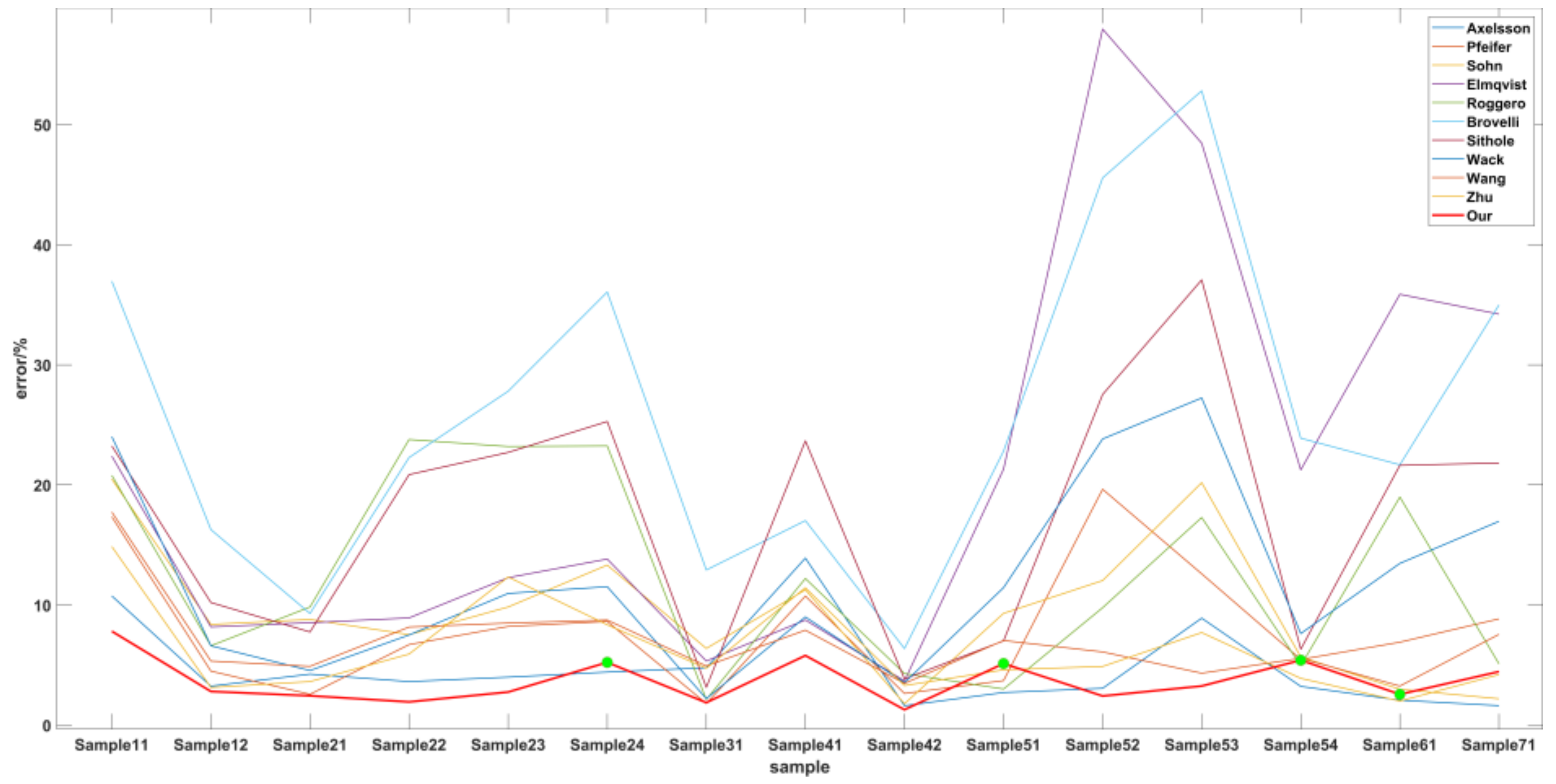
| Site | Sample | Axelsson [5] | Pfeifer [24] | Sohn [25] | Elmqvist [26] | Roggero [27] | Brovelli [28] | Sithole [2] | Wack [29] | Wang [9] | Zhu [8] | Our |
|---|---|---|---|---|---|---|---|---|---|---|---|---|
| Urban | 1-1 | 10.76 | 17.35 | 20.49 | 22.40 | 20.80 | 36.96 | 23.25 | 24.02 | 17.74 | 14.87 | 7.82 |
| 1-2 | 3.25 | 4.50 | 8.39 | 8.18 | 6.61 | 16.28 | 10.21 | 6.61 | 5.34 | 3.14 | 2.81 | |
| 2-1 | 4.25 | 2.57 | 8.8 | 8.53 | 9.84 | 9.30 | 7.76 | 4.55 | 4.90 | 3.63 | 2.45 | |
| 2-2 | 3.63 | 6.71 | 7.54 | 8.93 | 23.78 | 22.28 | 20.86 | 7.51 | 8.17 | 5.92 | 1.94 | |
| 2-3 | 4.00 | 8.22 | 9.84 | 12.28 | 23.20 | 27.80 | 22.71 | 10.97 | 8.50 | 12.34 | 2.76 | |
| 2-4 | 4.42 | 8.64 | 13.33 | 13.83 | 23.25 | 36.06 | 25.28 | 11.53 | 8.75 | 8.36 | 5.23 | |
| 3-1 | 4.78 | 1.80 | 6.39 | 5.34 | 2.14 | 12.92 | 3.15 | 2.21 | 4.93 | 4.74 | 1.88 | |
| 4-1 | 13.91 | 10.75 | 11.27 | 8.76 | 12.21 | 17.03 | 23.67 | 9.01 | 7.91 | 11.44 | 5.80 | |
| 4-2 | 1.62 | 2.64 | 1.78 | 3.68 | 4.30 | 6.38 | 3.85 | 3.54 | 3.48 | 3.30 | 1.29 | |
| Rural | 5-1 | 2.72 | 3.71 | 9.31 | 21.31 | 3.01 | 22.81 | 7.02 | 11.45 | 7.05 | 4.61 | 5.13 |
| 5-2 | 3.07 | 19.64 | 12.04 | 57.95 | 9.78 | 45.56 | 27.53 | 23.83 | 6.10 | 4.89 | 2.43 | |
| 5-3 | 8.91 | 12.60 | 20.19 | 48.45 | 17.29 | 52.81 | 37.07 | 27.24 | 4.33 | 7.71 | 3.26 | |
| 5-4 | 3.23 | 5.47 | 5.68 | 21.26 | 4.96 | 23.89 | 6.33 | 7.63 | 5.57 | 3.90 | 5.41 | |
| 6-1 | 2.08 | 6.91 | 2.99 | 35.87 | 18.99 | 21.68 | 21.63 | 13.47 | 3.26 | 2.01 | 2.57 | |
| 7-1 | 1.63 | 8.85 | 2.20 | 34.22 | 5.11 | 34.98 | 21.83 | 16.97 | 7.56 | 4.21 | 4.46 | |
| average | 4.82 | 8.02 | 9.35 | 20.73 | 12.34 | 25.78 | 17.48 | 12.04 | 6.91 | 6.34 | 3.68 | |
Disclaimer/Publisher’s Note: The statements, opinions and data contained in all publications are solely those of the individual author(s) and contributor(s) and not of MDPI and/or the editor(s). MDPI and/or the editor(s) disclaim responsibility for any injury to people or property resulting from any ideas, methods, instructions or products referred to in the content. |
© 2023 by the authors. Licensee MDPI, Basel, Switzerland. This article is an open access article distributed under the terms and conditions of the Creative Commons Attribution (CC BY) license (https://creativecommons.org/licenses/by/4.0/).
Share and Cite
Kang, C.; Lin, Z.; Wu, S.; Lan, Y.; Geng, C.; Zhang, S. A Triangular Grid Filter Method Based on the Slope Filter. Remote Sens. 2023, 15, 2930. https://doi.org/10.3390/rs15112930
Kang C, Lin Z, Wu S, Lan Y, Geng C, Zhang S. A Triangular Grid Filter Method Based on the Slope Filter. Remote Sensing. 2023; 15(11):2930. https://doi.org/10.3390/rs15112930
Chicago/Turabian StyleKang, Chuanli, Zitao Lin, Siyi Wu, Yiling Lan, Chongming Geng, and Sai Zhang. 2023. "A Triangular Grid Filter Method Based on the Slope Filter" Remote Sensing 15, no. 11: 2930. https://doi.org/10.3390/rs15112930