Article

Spatial Population Distribution Data Disaggregation Based on SDGSAT-1 Nighttime Light and Land Use Data Using Guilin, China, as an Example

1
International Research Center of Big Data for Sustainable Development Goals, Beijing 100094, China
2
Aerospace Information Research Institute, Chinese Academy of Sciences, Beijing 100101, China
3
University of Chinese Academy of Sciences, Beijing 100049, China
4
Key Laboratory of Digital Earth Science, Aerospace Information Research Institute, Chinese Academy of Sciences, Beijing 100094, China
*
Author to whom correspondence should be addressed.
Remote Sens. 2023, 15(11), 2926; https://doi.org/10.3390/rs15112926
Submission received: 9 April 2023 / Revised: 31 May 2023 / Accepted: 1 June 2023 / Published: 3 June 2023

Abstract

:
A high-resolution population distribution map is crucial for numerous applications such as urban planning, disaster management, public health, and resource allocation, and it plays a pivotal role in evaluating and making decisions to achieve the UN Sustainable Development Goals (SDGs). Although there are many population products derived from remote sensing nighttime light (NTL) and other auxiliary data, they are limited by the coarse spatial resolution of NTL data. As a result, the outcomes’ spatial resolution is restricted, and it cannot meet the requirements of some applications. To address this limitation, this study employs the nighttime light data provided by the SDGSAT-1 satellite, which has a spatial resolution of 10 m, and land use data as auxiliary data to disaggregate the population distribution data from WorldPop data (100 m resolution) to a high resolution of 10 m. The case study conducted in Guilin, China, using the multi-class weighted dasymetric mapping method shows that the total error during the disaggregation is 0.63%, and the accuracy of 146 towns in the study area is represented by an R2 of 0.99. In comparison to the WorldPop data, the result’s information entropy and spatial frequency increases by 345% and 1142%, respectively, which demonstrates the effectiveness of this approach in studying population distributions with high spatial resolution.

1. Introduction

The 2030 Agenda for Sustainable Development, which was adopted by all Member States of the United Nations in 2015, provides a comprehensive framework towards peace and prosperity for all humankind through the accomplishment of 17 Sustainable Development Goals (SDGs) [1]. High-resolution population distribution information is of critical importance for evaluation and decision-making in relation to the achievement of several of these SDG indicators at a fine resolution, such as those pertaining to traffic planning referring to SDG 11.2.1 [2,3], public health facilities construction referring to SDG 3.8.1 [4,5], and disaster prevention and response planning referring to SDG 11.5.1/11.5.2 [6,7,8,9].
Currently, there are two types of widely used population distribution data. The first is based on census statistics that are aggregated over administrative units, e.g., provinces, counties, townships, census tracts, or block groups [10]. However, these population data do not accurately represent the true spatial distribution of the population because spatial homogeneity exists in the census results of the administrative units of each region [11]. The second type of data is the disaggregated population product derived from remote sensing nighttime light (NTL) data and other auxiliary data [12,13,14,15], such as the Gridded Population of the World (GPW), WorldPop datasets, the Oak Ridge National Laboratory’s LandScan Population data, the European Commission Joint Research Centre (JRC) and CIESIN’s Global Human Settlement Population Layer (GHS-POP), ESRI’s World Population Estimate (WPE), Facebook and CIESIN’s High Resolution Settlement Layer (HRSL), JRC’s European GHS Population Grid, and the U.S. Census Bureau’s country grids (Demobase) [16]. Most of the current population distribution products were inversed from the DMSP/OLS or NPP/VIIRS data with spatial resolution around 1 km and 500 m, respectively [17,18,19,20]. Although several studies have tried adding other auxiliary data to improve the population data resolution and have formed some mature products (up to 100 m resolution so far) [21,22], spatial resolution is still limited due to the limited spatial resolution of NTL data. As a result, the current disaggregated population products may be insufficient to meet the demand for some applications, such as precise public resource allocation management and intelligent urban governance.
This paper focuses on developing a high spatial resolution population distribution dataset based on new satellite data, namely SDGSAT-1 NTL data, with a 10 m spatial resolution and land use data. The methods used for this task are generally divided into two categories [23]: top-down and bottom-up [24]. The bottom-up method involves using NTL data, ancillary data such as high-resolution imagery and land cover data, and sample survey or micro-census survey population data to predict the population of grids within non-surveyed areas. The objective of this method is to establish the quantitative relationship between survey population data, NTL data, and ancillary data which will enable it to create an accurate model for calculating the population of each grid [18]. Nonetheless, because of regional disparities in economic level and social environment, the population distribution data vary significantly and necessitate an extensive sample size to achieve the desired model accuracy [25]. Furthermore, using a single linear model may not meet the requirements of the entire study area, resulting in substantial errors in the final population spatial distribution map. Therefore, this method is commonly used to map population distribution in large regions with a low spatial resolution. The top-down method involves using mathematical models to convert population statistical data from irregular administrative units into regular grids such as cells or pixels. Population disaggregation is another term for this process. In disaggregation methods, population statistical data and administrative boundaries serve as the fundamental input data. Disaggregation methods fall into three categories: binary dasymetric, multi-class dasymetric, and intelligent dasymetric mapping [23]. Binary dasymetric mapping divides source zones into two sub-zones [26], typically populated and unpopulated areas, through the use of ancillary data. However, this method lacks the accuracy and precision necessary for accurately and thoroughly mapping population distribution. Intelligent dasymetric mapping, on the other hand, uses complex models, particularly machine learning, to create spatialized population distribution. Deep learning is a recent development in the mapping of population distribution and has shown promising results [27,28]. However, practical applications of this method can be challenging due to the large number of required training datasets. As a result, there are limits to the utilization of this method. Mennis (2003) [29] proposed the multi-class weighted dasymetric mapping method based on binary dasymetric mapping. The multi-class weighted dasymetric mapping method divides population areas into additional subcategories based on their different population densities, assigning different weights to each subcategory to determine the regional population density. In this paper, we apply the multi-class weighted dasymetric mapping method and use SDGSAT-1 NTL data with a 10 m spatial resolution and land use data to disaggregate the existing WorldPop 100 m population dataset to a 10 m spatial resolution, focusing on the study area of Guilin, China.
The remainder of this paper is structured as follows: Section 2 provides an introduction to the study area of Guilin, China, elaborates on the dataset utilized, the methodology employed, and the evaluation indicators. Section 3 proceeds with the analysis and discussion of the experimental results. Finally, Section 4 summarizes the findings of this study.

2. Materials and Methods
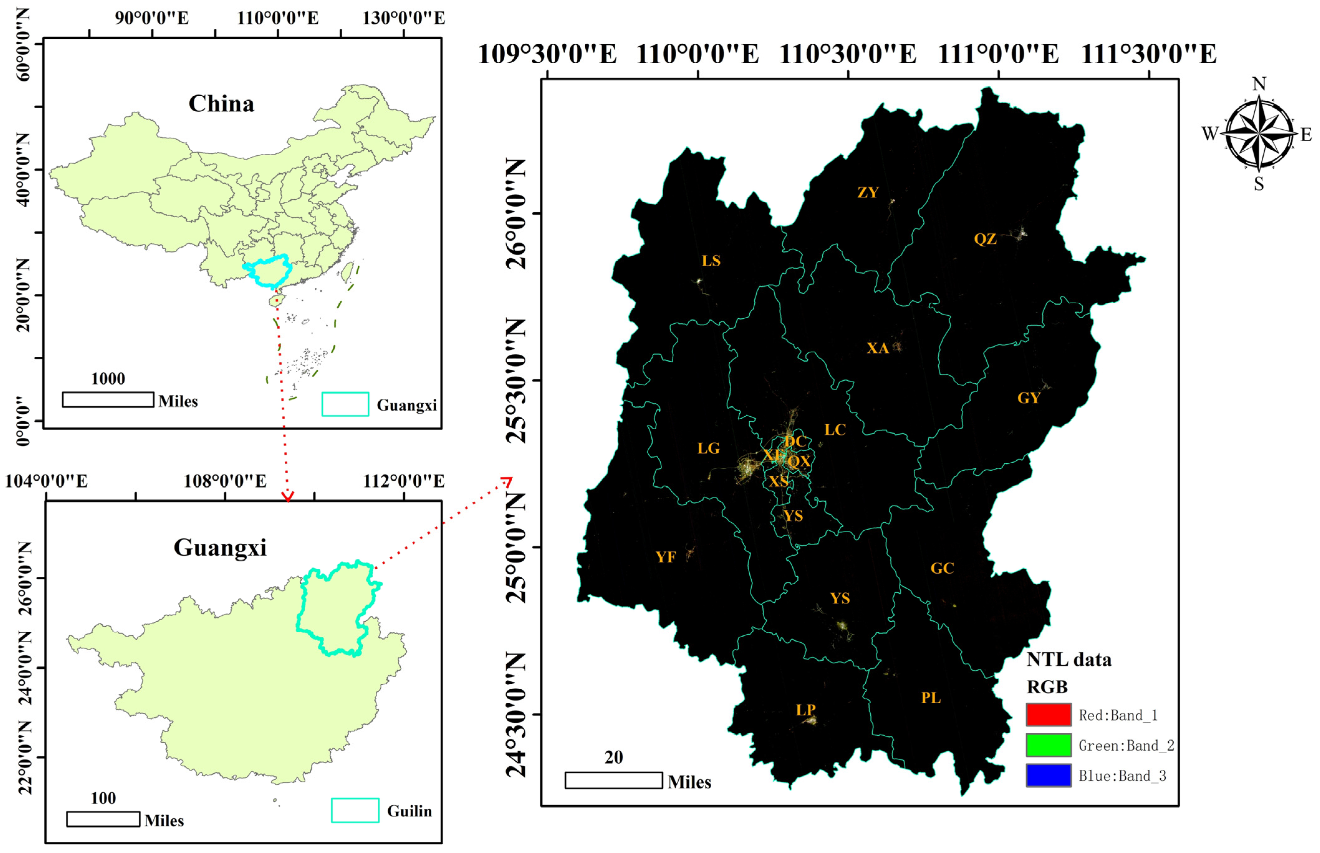
2.1. Study Area

In this study, we selected Guilin city, which is situated in the northeast of Guangxi Zhuang Autonomous Region in South China, as our study area. The city’s coordinates are 109°36′50″E to 111°29′30″E and 24°15′23″N to 26°23′30″N. It is 236 km long from north to south and 189 km wide from east to west (Figure 1). Guilin comprises six administrative districts, namely Xiufeng, Duocai, Xiangshan, Qixing, Yanshan, and Linggui, and ten counties (autonomous counties), including Yangshuo, Lingchuan, Quanzhou, Xing’an, Yongfu, Guanyang, Longsheng, Ziyuan, Pingle, Gongcheng, and Lipu City.

2.2. Data Sources

NTL and land use data are introduced as auxiliary data to disaggregate the existing coarse population product in this study. The basic information of these data is shown in Table 1.

2.2.1. Population Products

Population data suitable for fine-scale applications are developed by WorldPop using a large amount of ancillary data layers. The dataset is global in scope and covers the years 2010 to 2020, making it highly accessible for subsequent studies. The WorldPop dataset provides products with resolutions of 1 km and 100 m, as depicted in Figure 2 for Guilin, China.

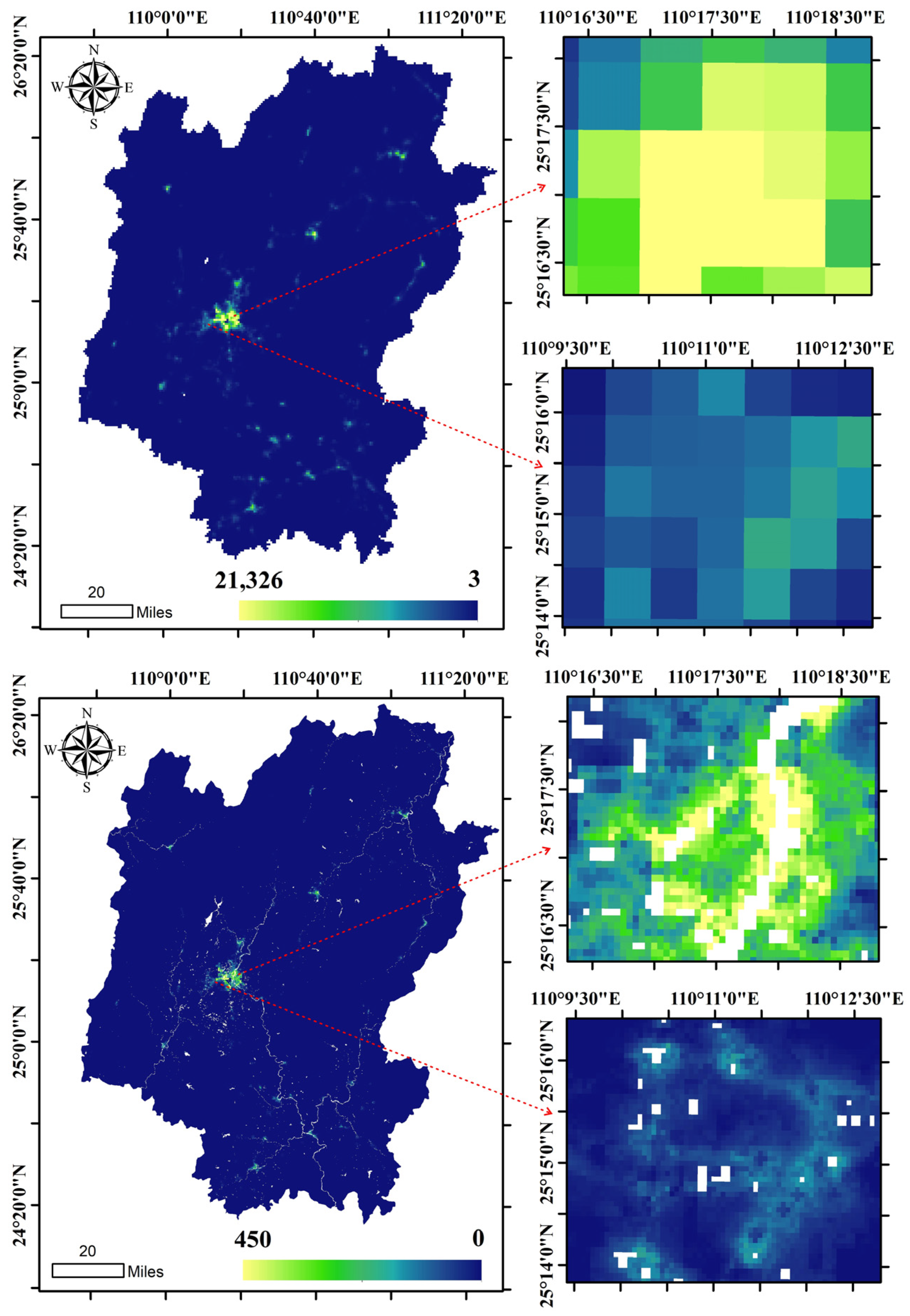
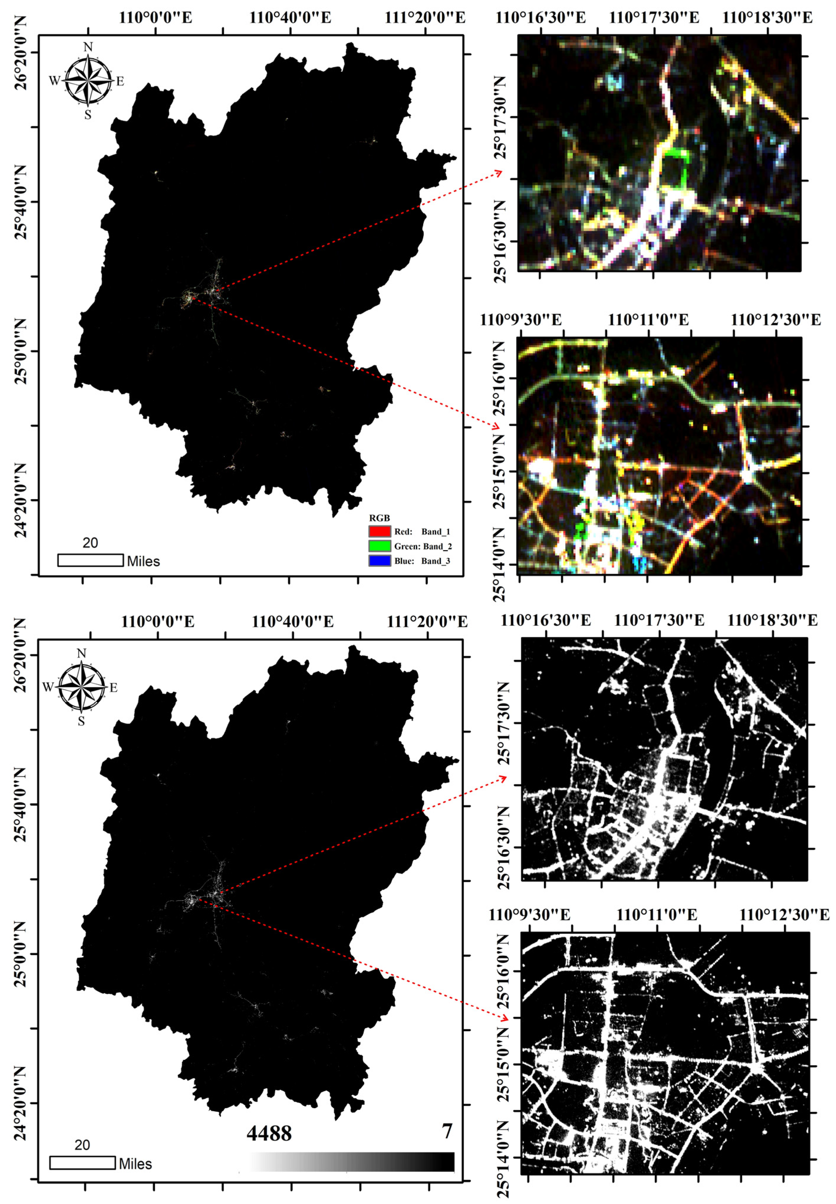
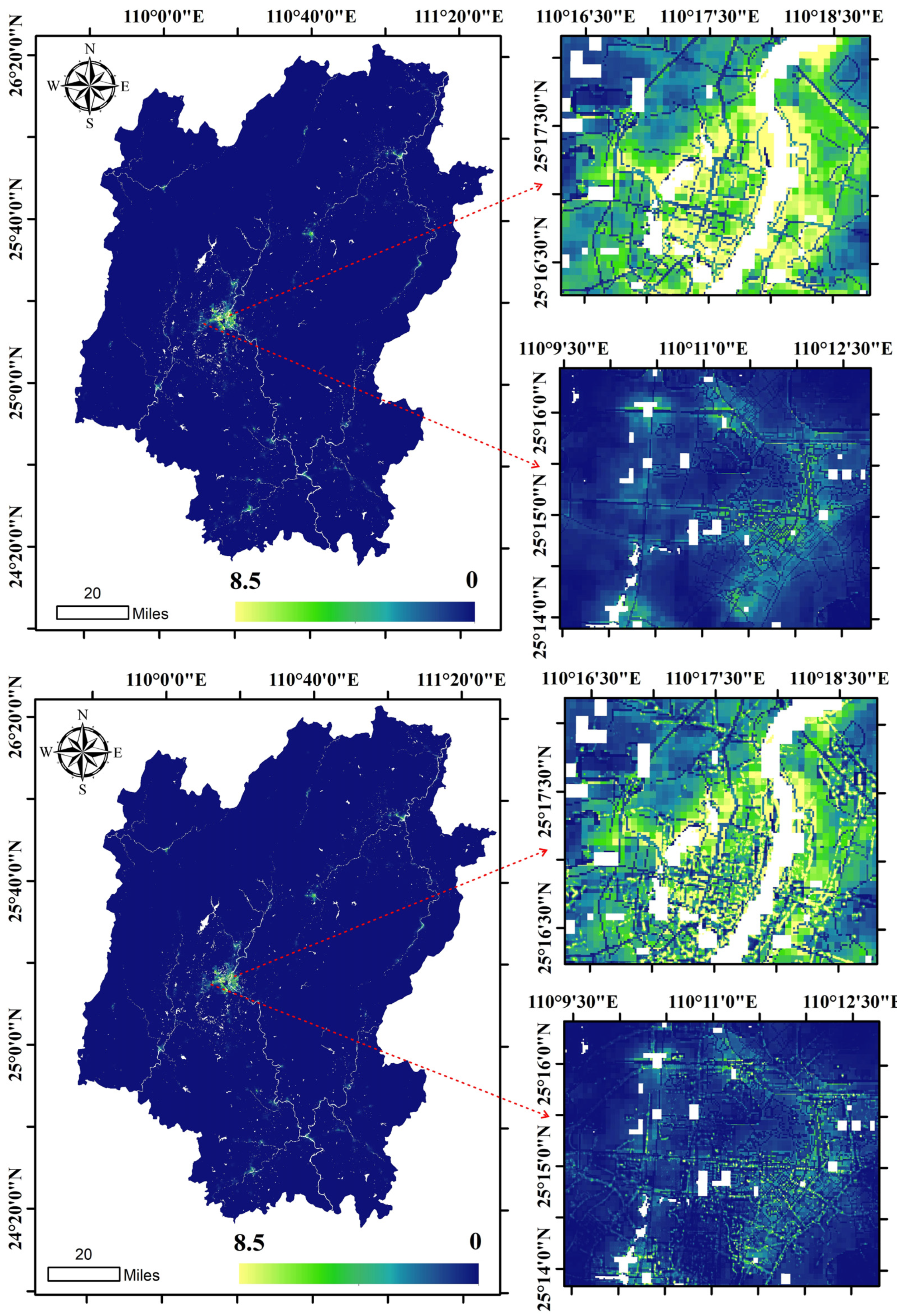
2.2.2. Nighttime Light Data

At present, there are three primary types of NTL data available in the global scale: (1) DMSP/OLS data, which span 1992 to 2013 with 1 km spatial resolution; (2) NPP/VIIRS data, covering 2013 to 2019 at 500 m spatial resolution; and (3) Luojia-01 NTL data, launched on 2 June 2018, with 130 m spatial resolution.
The Chinese Academy of Sciences (CAS) launched the Sustainable Development Goals Satellite-1 (SDGSAT-1) into orbit on 5 November 2021. It is the first satellite designed specifically to implement the United Nations 2030 Agenda for Sustainable Development and the first earth science satellite developed by the CAS. Table 2 displays the main parameters of the satellite. The satellite’s NTL data comprise four bands, including three visible light bands and one panchromatic band with a maximum spatial resolution of 10 m.
SDGSAT-1 data products consist of Level 1, Level 2, and Level 4 data. Level 1 data products are generated by processing relative radiation correction, band registration, HDR fusion, and RPC on the basis of level 0 products, resulting in standard products. Level 2 data products are the geometrically corrected versions of the Level 1 standard products. Level 4 data products result from thorectifying the Level 1 standard products using ground control points, digital elevation models, and in accordance with format specifications. We used only Level 4 products in this study since they are currently the only products available to users. Figure 3 shows that a true-color synthesis image allows us to clearly distinguish the contour of roads and buildings as well as the color of ground neon lights.

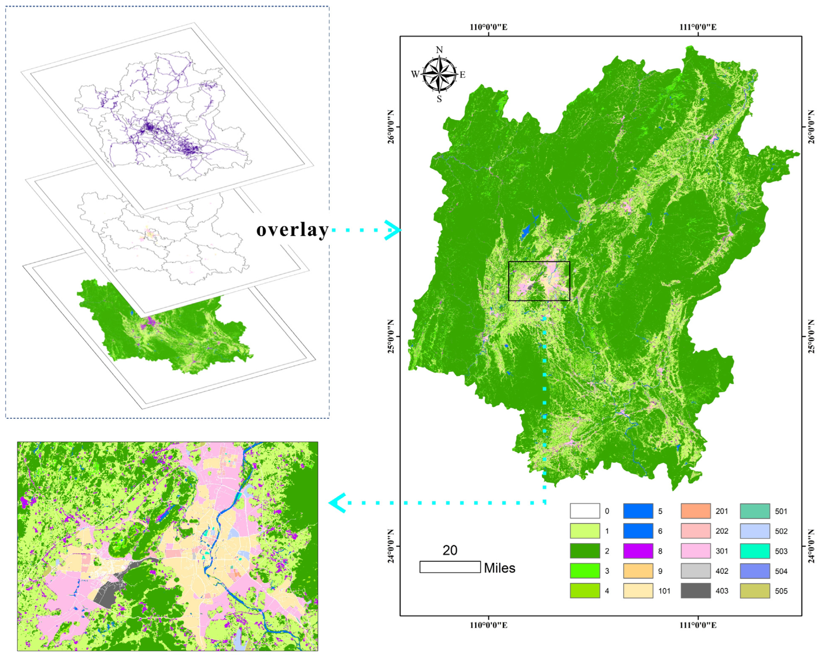
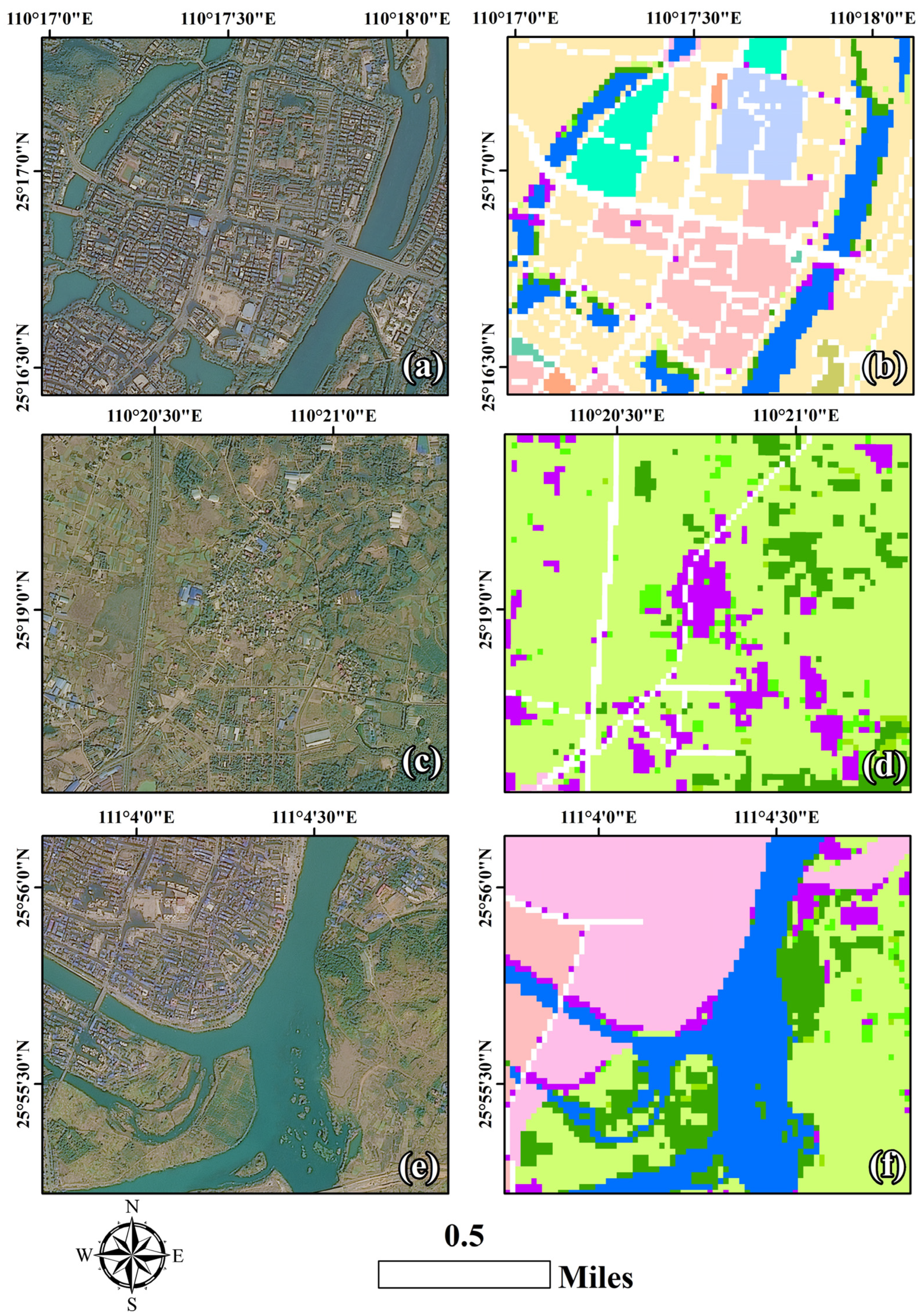
2.2.3. Land Use Data

In this study, we used three auxiliary land use datasets: EULUC-China data, FROM-GCL10 data, and road network data. The EULUC-China dataset, generated by Tsinghua University, utilizes 10-m resolution satellite imagery (Sentinel-2A/B) from 2018, OpenStreetMap, night lights (Luojia1-01), POI (Amap, POI category and quantity), and Tencent mobile-phone locating-request (MLP) data (i.e., 8-h mean trajectories of the active population during weekdays and weekends) to produce a dataset containing 440,798 plots labeled with five primary and twelve subcategory feature labels in major Chinese cities [30]. It is not feasible to use the same classification scheme for both urban and rural areas due to their different environments. Hence, we employed FROM-GCL10, developed by Tsinghua University, which is the world’s first 10-m resolution global surface coverage product with 72.76% overall accuracy [31]. This product uses a random forest classifier on the Google Earth Engine platform to map global land cover at a 10-m resolution by transferring the 30-m resolution sample set from 2015 to the Sentinel-2 imagery acquired in 2017. The surface features include cropland, forest, grassland, shrubland, wetland, water, tundra, impervious, barren, and snow/ice. Notably, in our study, impervious ground in rural areas is considered as villages. The road network data of the study area were obtained from OpenStreetMap (www.openstreetmap.org, OSM) (accessed on 6 March 2018), an open-source map which includes road layers such as highways, urban expressways, main roads, secondary roads, branch roads, country roads, bicycle roads, pedestrian roads, and internal roads.
The EULUC-China dataset furnishes a sound classification of functional area in urban areas but fails to include data pertaining to types of roads. As a result, the OSM data were utilized to create a 20 m buffer zone, which was then superimposed on the EULUC-China data to augment the latter. The EULUC-China and road network data (both as vectors) are transformed into 10 m raster data to comply with the experimental requirements. As the road network is not the main area of population distribution, we opted not to divide the various roads. Figure 4 illustrates the EULUC-China, FROM-GCL10, and road network data layers were stacked together using the ArcGIS 10.3 software to form a comprehensive land use data set for the study area. Three typical areas characterized as urban, rural, and urban–rural interface were chosen for comparison, with SDGSAT-1 multispectral data to confirm the accuracy of land use data. Figure 5 reveals a high level of agreement between each area type and the remote sensing data.
In the first round of disaggregation, land use data are incorporated.

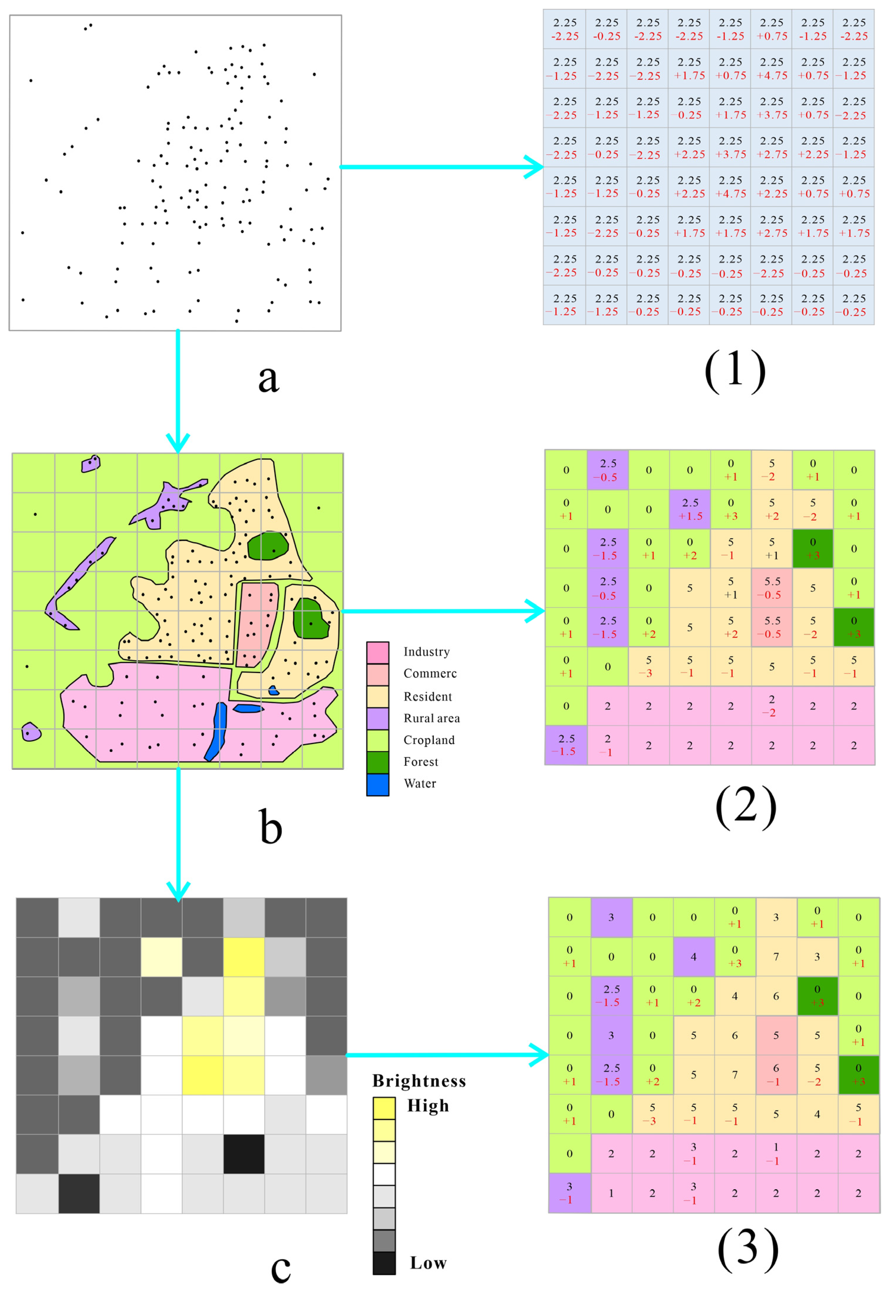
2.3. Multi-Class Weighted Dasymetric Mapping

In this study, we employed a multi-class weighted dasymetric mapping method for population disaggregation. This method was first named by Semenov-Tian-Shansky in 1928 [32] and developed by many scholars [25,29]; it subdivides populated areas into subcategories based on factors such as land use and infrastructure density, reflecting different population densities. By applying different weighting factors to each category, we obtained a more realistic population distribution [25]. This method is widely utilized in population disaggregation and often regarded as the most effective approach [33]. The flow diagram of this method is shown in Figure 6. Our initial premise was that a square area contains 144 individuals and that the optimal representation of their distribution is individual points, as shown in Figure 6a. Nonetheless, it is arduous and expensive to obtain data on individuals, so we divided the study area into grids of uniform size to approximate the practical situation as closely as possible. In the absence of additional auxiliary data, we assumed that the population in an area is evenly distributed. However, as evidenced in Figure 6(1), this approach led to a considerable deviation from the actual population distribution. Additionally, the grids varied in their level of deviation from one another, indicating the presence of spatial heterogeneity in population distribution.
To account for regional disparities, we integrated land use data, as illustrated in Figure 6b. The quantity of individuals in distinct land use categories varied, and we allocated each land use type a corresponding distribution coefficient. We then employed these coefficients to ascertain the population distribution in each land use type (Formula (1)). Consequently, the total number of individuals in each grid was determined by proportioning the individuals across land use types calculated to be in each grid (Formula (2)). As Figure 6(2) demonstrates, incorporating land use data considerably reduced the number of grids that deviated from the actual population distribution, demonstrating the effectiveness of our approach in reflecting regional differences in population distribution.
W j = D j D
where W j is the population distribution coefficient of the jth land use type, D j is the population density of the jth land use type, and D is the total population density.
P ij = P i × W j j = 1 n W j
where P i is the population of the ith disaggregation unit, P ij is the population of the jth land use type in the ith decomposition unit, and W j is the population distribution coefficient of the jth land use type
Despite considering land use type, varying degrees of deviation still existed, indicating persistent spatial heterogeneity. To address this issue, we introduced NTL data, as shown in Figure 6c. NTL data can sensitively capture and record human activities [30], and a significant positive correlation between nighttime lights and population has been demonstrated in numerous countries and regions [19]. In this paper, we leveraged NTL data to redistribute the population of the same land use type within each disaggregation unit (Formula (3)) to replace the previous average distribution. Nevertheless, it was vital to note that nighttime lights can be influenced by numerous factors, including the economy, culture, climate, season, government management system, and more. For instance, in some less developed areas, low nighttime light intensity does not necessarily indicate a small population distribution. To minimize deviations between the population disaggregation results and reality caused by such fluctuations, we aimed to minimize the disaggregation units’ size. Figure 6(3) displays the final outcome, demonstrating a further reduction in the number of grids that deviated from the actual population distribution compared to Figure 6(2).
P ij = P i × L j j = 1 n L j
where P i is the population of the ith land use type in each disaggregation unit, P ij is the population of the jth pixel in the ith land use type in each decomposition unit, and L j is the brightness value of the jth pixel in the ith land use type in each disaggregation unit.

2.4. Evaluation Indicators

Accuracy verification has always been a challenging task in population distribution studies. Currently, three primary methods can ascertain model accuracy. The first involves comparing disaggregation results with census data [18]. The second method utilizes geospatial measures such as relative error and root mean square error (RMSE) to assess population disaggregation results and existing population products’ differences in spatial structure and correlation between [34]. In our study, the WorldPop products are used as the input data for population disaggregation to generate higher spatial resolution population data than the original product. The accuracy of the disaggregation results relies heavily on the quality of the population products. Therefore, to a certain extent, accuracy can be guaranteed. The third method involves field sampling surveys, which are only applicable for small-scale research. In conclusion, the first and third methods are not essential in this study, and the relative error is used as the evaluation indicator (Formula (4)) to assess the model’s accuracy.
E r r o r = ( pop ~ pop / p o p )
where pop ~ is the population of the disaggregation result, and pop is the population of the existing population products.
Additionally, another two objective indicators were introduced to evaluate the fineness of the disaggregation result in our study, namely, information entropy (IE) and spatial frequency (SF). IE of an image measures its statistical characteristics, indicating the average amount of information present in the image and representing the aggregation feature of image gray distribution (Formula (5)). IE is used to verify the improvement of the disaggregation result in the amount of information it contains. SF reflects the rate of change in raster data value (Formulas (6)–(8)) and can be used to evaluate the spatial resolution of the data. At the same scale, a higher IE represents a greater the amount of information, and a higher SF indicates higher spatial resolution and a clearer image.
H X = i = 1 m P i X log 2 P i X
where H X is information entropy, and P i X is the probability of occurrence of each gray level.
S F F = RF 2 + CF 2
R F = 1 MN i = 1 M j = 1 N   H i , j H i , j 1
C F = 1 MN i = 1 M j = 1 N   H i , j H i 1 , j
where M and N are the width and height of the image, respectively, and H i , j is the pixel value of the i,j coordinates.

3. Results

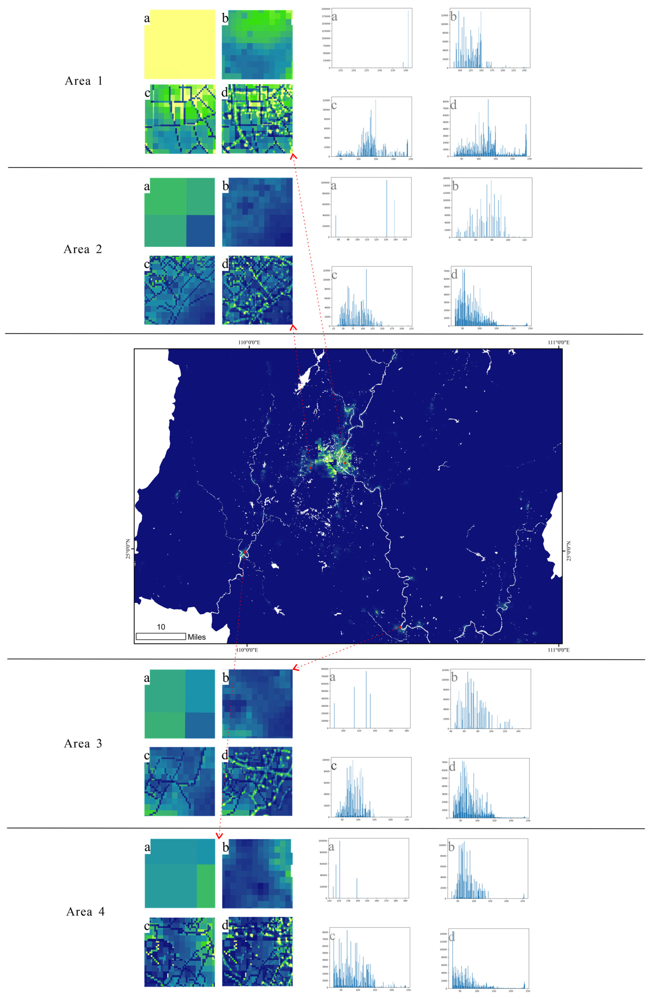
3.1. Result of the Disaggregation

The coefficient of population distribution for each land use type was calculated using the WorldPop 100 m population data and Formula (1). Subsequently, adjustments to the coefficient values were made based on actual conditions. Table 3 reveals that the coefficients in urban areas are higher than those in rural areas. Due to the high brightness false information caused by the specular reflection of bodies of water during the acquisition process of satellite nighttime lighting data, we manually adjusted the weight of water and wetland values to 0.
Each 100 m grid is disaggregated into multiple land use types, serving as an independent disaggregation unit. Using distribution coefficients, the disaggregation unit’s population is redistributed among different land use types within the unit. Figure 7 displays the outcome of the initial disaggregation. By incorporating land use data, the distribution pattern of the population in the disaggregation unit varying with socioeconomic activities has been accurately captured. The population is predominantly concentrated in urban areas. In addition, the population density varies within the different functional areas of urban areas. For example, residential areas, commercial areas, and hospitals have high population density, whereas industrial areas have comparatively low population density. Generally, the population density in rural areas is lower than that in urban areas. It is primarily concentrated in villages. Lake and river areas do not have a population distribution owing to subjective correction.
Following the initial disaggregation, we discover that the population within areas of the same land use type is uniformly distributed, causing significant deviation. To improve the uniformity of population distribution in areas of the same land use type within each disaggregation unit, NTL data will be incorporated. SDGSAT-1 NTL data provides a 10 m resolution that can sensitively capture and record human activities. Nighttime light brightness reflects the degree of population concentration, and the brighter areas of the same land use type indicate denser population distribution. Figure 7 depicts the outcome of the disaggregation. In comparison to Figure 2, the population distribution pattern shown in Figure 7 is a closer approximation to the real population distribution, providing a more detailed insight. Regardless of the land use type, the population is typically clustered, particularly in urban areas. However, variations exist within different blocks due to the restrictions imposed by social, economic, and cultural factors.

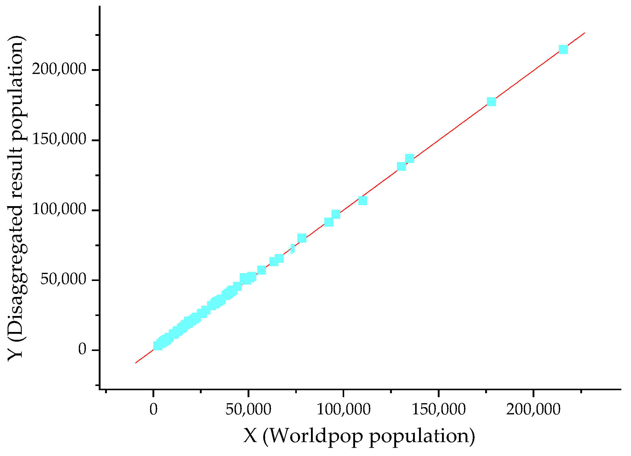
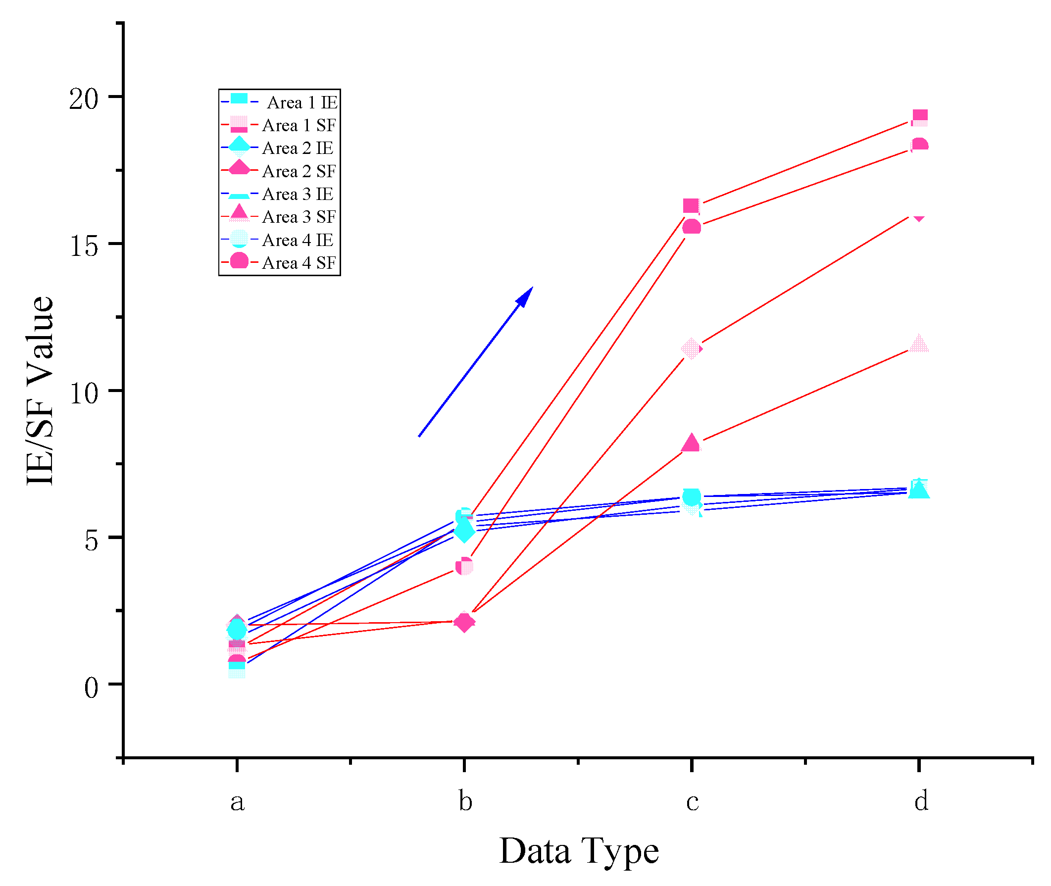
3.2. Accuracy Evaluation

For validating the effectiveness of the proposed method, it is crucial to assess the disaggregation results’ accuracy. For the analysis, 17 districts and counties within the study area were taken as units for analysis. The population of each district or county in the WorldPop data and disaggregation result of the study area were counted, and then the relative error was calculated using Formula (4). Table 4 shows that except for a few individual districts and counties, the relative error is less than 2%, with a total relative error of only 0.63%. Furthermore, to assess the reliability further, 146 towns in the study area were analyzed, and the population of each town in the WorldPop data and the disaggregation result of the study area were counted. As shown in Figure 8, all points are in close proximity to the trend line with minimal error and an R2 value of 0.99. The high degree of consistency between the disaggregation results’ accuracy and that of the disaggregation data validates the proposed method, confirming that it does not undermine the accuracy of the results.
Following the confirmation of the accuracy of the disaggregation result, we introduced objective indicators to evaluate the refinement of the result. We selected four urban areas in Guilin with a significant population distribution that were then adjusted to the same size for evaluation purposes. Histogram statistics were then performed on the selected areas, and the values of IE and SF were calculated for each area (see Figure 9 and Table 5). As a result, the information entropy increased by 345%, and the spatial frequency rose by 1142%, as depicted in Figure 10.
A subjective evaluation was carried out by scaling up the four types of population grid data to 1:10,000 in four different areas. At this scale, a strong mosaic phenomenon was observed, regardless of whether it was the WorldPop population grid data with a spatial resolution of 1 km or 100 m. Nevertheless, the two disaggregation results generated by this study substantially ameliorated this issue. Notably, the outcome of the first disaggregating land use data could clearly identify the distinct distribution of population across diverse functional locations of the city. Furthermore, utilizing SDGSAT-1 NTL data to disaggregate the population grid data led to the emergence of numerous bright spots in multiple functional areas, signifying the dense concentration of population in those areas. Figure 9 depicts population grid data for the four areas ranging from 1 km to 100 m in the first round of disaggregation, and later in the final disaggregation, respectively. The information entropy (IE) value and spatial frequency (SF) value both increased monotonically, which was consistent with our subjective visual evaluation results. Based on the significance of the numerical values of IE and SF, the effectiveness of this study in addressing the problem of improving the spatial resolution of population grid data was further objectively verified.

4. Conclusions and Discussion

In this study, we focused on Guilin, China, as the study area and used the WorldPop population data as the input data, supplemented by SDGSAT-1 NTL data and land use data to generate a population distribution grid with a spatial resolution of 10 m using the multi-class dasymetric mapping method. SDGSAT-1 NTL data were introduced for the first time in the context of population disaggregation. Based on the results of disaggregation and accuracy verification, we found that the spatial resolution of the output was significantly improved while maintaining accuracy, and the output had better performance in detail. This demonstrates the effectiveness of this approach in studying population distributions with high spatial resolution.
However, the ground accuracy of the disaggregation results heavily relies on the accuracy of the input data (WorldPop data in this study). In general, the accuracy and spatial resolution of the disaggregation results increase with higher accuracy of input data and auxiliary data. Although WorldPop has been widely used, the total population statistics are not always consistent with the census data, particularly at the small local administrative scale. We utilized the WorldPop 100 m data because it is the highest spatial resolution population distribution data available in the study area. To generate a population disaggregation model at a higher spatial resolution (10 m), a large number of samples at small spatial units were required. Unfortunately, the census data in the study area did not provide sufficient support for this purpose. As this paper mainly focuses on the disaggregation method of high spatial resolution population distribution, the WorldPop population grid data product is finally selected as the input source data for our model. Future studies may explore generating high resolution population grid data disaggregation models based on the ground truth data. On the other hand, WorldPop’s grid values are not continuously changing; there are varying degrees of abruptness in these discrete values which result in obvious boundaries in the disaggregation results. Additionally, in this study, only NTL data and land use data were utilized as auxiliary data, while other data such as building footprints [15], building volume [35], points of interest (POI) [14,36], and GPS tracking data [37] could reflect the spatial heterogeneity of population distribution and contribute to fine population disaggregation. In the study of population distribution with high spatial resolution, improving the accuracy of the model remains a challenge due to the lack of more precise population samples.

Author Contributions

Conceptualization: C.L. and Y.C.; methodology: C.L. and Y.C.; writing—original draft preparation: C.L.; writing—review and editing: Y.C., Y.W. and F.C.; funding acquisition: Y.C. and F.C.; All authors have read and agreed to the published version of the manuscript.

Funding

This research was funded by the National Natural Science Foundation of China (42271422), the Strategic Priority Research Program of the Chinese Academy of Sciences (grant number XDA19090132), and National Key R&D Program of China (Project No. 2022YFC3800700).

Data Availability Statement

All data are available in the main text.

Acknowledgments

We express our gratitude to SDGSAT-1 Open Science Program for providing NLD data for this study.

Conflicts of Interest

The authors declare no conflict of interest.

References

  1. Nations, U. Transforming Our World: The 2030 Agenda for Sustainable Development; United Nations: New York, NY, USA, 2015. [Google Scholar]
  2. Jochem, W.C.; Sims, K.; Bright, E.A.; Urban, M.L.; Rose, A.N.; Coleman, P.R.; Bhaduri, B.L. Estimating traveler populations at airport and cruise terminals for population distribution and dynamics. Nat. Hazards 2013, 68, 1325–1342. [Google Scholar] [CrossRef]
  3. UNGGIM. Geospatial Industry Advancing Sustainable Development Goals; Geospatial Media and Communications: Noida, India, 2021. [Google Scholar]
  4. Makinde, O.A.; Sule, A.; Ayankogbe, O.; Boone, D. Distribution of health facilities in Nigeria: Implications and options for Universal Health Coverage. Int. J. Health Plan. Manag. 2018, 33, E1179–E1192. [Google Scholar] [CrossRef] [PubMed]
  5. Kuupiel, D.; Adu, K.M.; Apiribu, F.; Bawontuo, V.; Adogboba, D.A.; Ali, K.T.; Mashamba-Thompson, T.P. Geographic accessibility to public health facilities providing tuberculosis testing services at point-of-care in the upper east region, Ghana. BMC Public Health 2019, 19, 718. [Google Scholar] [CrossRef] [Green Version]
  6. Aubrecht, C.; Özceylan, D.; Steinnocher, K.; Freire, S. Multi-level geospatial modeling of human exposure patterns and vulnerability indicators. Nat. Hazards 2013, 68, 147–163. [Google Scholar] [CrossRef]
  7. Li, S.; Schlebusch, C.; Jakobsson, M. Genetic variation reveals large-scale population expansion and migration during the expansion of Bantu-speaking peoples. Proc. R. Soc. B-Biol. Sci. 2014, 281, 20141448. [Google Scholar] [CrossRef] [PubMed] [Green Version]
  8. Cui, Y.; Li, S.J.; Wu, W.; Huang, H.; Liu, M. The application of residential distribution monitoring based on GF-1 images. In Proceedings of the 9th International Symposium on Multispectral Image Processing and Pattern Recognition (MIPPR)—Multispectral Image Acquisition, Processing, and Analysis, Enshi, China, 31 October–1 November 2015. [Google Scholar]
  9. Freire, S.; Aubrecht, C.; Wegscheider, S. Advancing tsunami risk assessment by improving spatio-temporal population exposure and evacuation modeling. Nat. Hazards 2013, 68, 1311–1324. [Google Scholar] [CrossRef]
  10. Yang, X.C.; Ye, T.T.; Zhao, N.Z.; Chen, Q.; Yue, W.Z.; Qi, J.G.; Zeng, B.; Jia, P. Population Mapping with Multisensor Remote Sensing Images and Point-Of-Interest Data. Remote Sens. 2019, 11, 574. [Google Scholar] [CrossRef] [Green Version]
  11. Chen, J.D.; Fan, W.; Li, K.; Liu, X.; Song, M.L. Fitting Chinese cities’ population distributions using remote sensing satellite data. Ecol. Indic. 2019, 98, 327–333. [Google Scholar] [CrossRef]
  12. Ma, T. Multi-Level Relationships between Satellite-Derived Nighttime Lighting Signals and Social Media-Derived Human Population Dynamics. Remote Sens. 2018, 10, 1128. [Google Scholar] [CrossRef] [Green Version]
  13. Bai, Z.Q.; Wang, J.L. Generation of High Resolution Population Distribution Map in 2000 and 2010: A Case Study in the Loess Plateau, China. In Proceedings of the 23rd International Conference on Geoinformatics (Geoinformatics), Wuhan, China, 19–21 June 2015. [Google Scholar]
  14. Bakillah, M.; Liang, S.; Mobasheri, A.; Arsanjani, J.J.; Zipf, A. Fine-resolution population mapping using OpenStreetMap points-of-interest. Int. J. Geogr. Inf. Sci. 2014, 28, 1940–1963. [Google Scholar] [CrossRef]
  15. Palacios-Lopez, D.; Bachofer, F.; Esch, T.; Heldens, W.; Hirner, A.; Marconcini, M.; Sorichetta, A.; Zeidler, J.; Kuenzer, C.; Dech, S.; et al. New Perspectives for Mapping Global Population Distribution Using World Settlement Footprint Products. Sustainability 2019, 11, 6056. [Google Scholar] [CrossRef] [Green Version]
  16. Leyk, S.; Gaughan, A.E.; Adamo, S.B.; de Sherbinin, A.; Balk, D.; Freire, S.; Rose, A.; Stevens, F.R.; Blankespoor, B.; Frye, C.; et al. The spatial allocation of population: A review of large-scale gridded population data products and their fitness for use. Earth Syst. Sci. Data 2019, 11, 1385–1409. [Google Scholar] [CrossRef] [Green Version]
  17. Li, K.N.; Chen, Y.H.; Li, Y. The Random Forest-Based Method of Fine-Resolution Population Spatialization by Using the International Space Station Nighttime Photography and Social Sensing Data. Remote Sens. 2018, 10, 1650. [Google Scholar] [CrossRef] [Green Version]
  18. Li, S.; Zhao, C.W. Study on Population Spatialization of Henan Province Based on Land Use and DMSP/OLS Data. J. Nat. Sci. Hunan Norm. Univ. 2019, 42, 9–15. [Google Scholar]
  19. Sun, W.C.; Zhang, X.; Wang, N.; Cen, Y. Estimating Population Density Using DMSP-OLS Night-Time Imagery and Land Cover Data. IEEE J. Sel. Top. Appl. Earth Observ. Remote Sens. 2017, 10, 2674–2684. [Google Scholar] [CrossRef]
  20. Li, X.M.; Zhou, W.Q. Dasymetric mapping of urban population in China based on radiance corrected DMSP-OLS nighttime light and land cover data. Sci. Total Environ. 2018, 643, 1248–1256. [Google Scholar] [CrossRef]
  21. Lloyd, C.T.; Chamberlain, H.; Kerr, D.; Yetman, G.; Pistolesi, L.; Stevens, F.R.; Gaughan, A.E.; Nieves, J.J.; Hornby, G.; MacManus, K. Global spatio-temporally harmonised datasets for producing high-resolution gridded population distribution datasets. Big Earth Data 2019, 3, 108–139. [Google Scholar] [CrossRef] [PubMed] [Green Version]
  22. Stevens, F.R.; Gaughan, A.E.; Linard, C.; Tatem, A.J. Disaggregating Census Data for Population Mapping Using Random Forests with Remotely-Sensed and Ancillary Data. PLoS ONE 2015, 10, 22. [Google Scholar] [CrossRef] [Green Version]
  23. Wardrop, N.A.; Jochem, W.C.; Bird, T.J.; Chamberlain, H.R.; Clarke, D.; Kerr, D.; Bengtsson, L.; Juran, S.; Seaman, V.; Tatem, A.J. Spatially disaggregated population estimates in the absence of national population and housing census data. Proc. Natl. Acad. Sci. USA 2018, 115, 3529–3537. [Google Scholar] [CrossRef] [Green Version]
  24. Qiu, Y.; Zhao, X.S.; Fan, D.Q.; Li, S.N.; Zhao, Y.J. Disaggregating population data for assessing progress of SDGs: Methods and applications. Int. J. Digit. Earth 2022, 15, 2–29. [Google Scholar] [CrossRef]
  25. Su, M.D.; Lin, M.C.; Hsieh, H.I.; Tsai, B.W.; Lin, C.H. Multi-layer multi-class dasymetric mapping to estimate population distribution. Sci. Total Environ. 2010, 408, 4807–4816. [Google Scholar] [CrossRef] [PubMed]
  26. Eicher, C.L.; Brewer, C.A. Dasymetric Mapping and Areal Interpolation: Implementation and Evaluation. Am. Cartogr. 2001, 28, 125–138. [Google Scholar] [CrossRef]
  27. Gervasoni, L.; Fenet, S.; Perrier, R.; Sturm, P. Convolutional neural networks for disaggregated population mapping using open data. In Proceedings of the 5th IEEE International Conference on Data Science and Advanced Analytics (IEEE DSAA), Turin, Italy, 1–4 October 2018; pp. 594–603. [Google Scholar]
  28. Monteiro, J.; Martins, B.; Murrieta-Flores, P.; Pires, J.M. Spatial Disaggregation of Historical Census Data Leveraging Multiple Sources of Ancillary Information. Isprs Int. J. Geo-Inf. 2019, 8, 327. [Google Scholar] [CrossRef] [Green Version]
  29. Mennis, J. Generating Surface Models of Population Using Dasymetric Mapping. Prof. Geogr. 2003, 55, 31–42. [Google Scholar] [CrossRef]
  30. Gong, P.; Chen, B.; Li, X.C.; Liu, H.; Wang, J.; Bai, Y.Q.; Chen, J.M.; Chen, X.; Fang, L.; Feng, S.L.; et al. Mapping essential urban land use categories in China (EULUC-China): Preliminary results for 2018. Sci. Bull. 2020, 65, 182–187. [Google Scholar] [CrossRef] [Green Version]
  31. Gong, P.; Liu, H.; Zhang, M.N.; Li, C.C.; Wang, J.; Huang, H.B.; Clinton, N.; Ji, L.Y.; Li, W.Y.; Bai, Y.Q.; et al. Stable classification with limited sample: Transferring a 30-m resolution sample set collected in 2015 to mapping 10-m resolution global land cover in 2017. Sci. Bull. 2019, 64, 370–373. [Google Scholar] [CrossRef] [Green Version]
  32. Semenov-Tian-Shansky, B. Russia: Territory and Population: A Perspective on the 1926 Census. Geogr. Rev. 1928, 18, 616–640. [Google Scholar] [CrossRef]
  33. Gallego, F.J.; Batista, F.; Rocha, C.; Mubareka, S. Disaggregating population density of the European Union with CORINE land cover. Int. J. Geogr. Inf. Sci. 2011, 25, 2051–2069. [Google Scholar] [CrossRef]
  34. Tan, M.; Liu, K.; Liu, L.; Zhu, Y.; Wang, D. Spatialization of population in the Pearl River Delta in 30 m grids using random forest model. Prog. Geogr. 2017, 36, 1304–1312. [Google Scholar]
  35. Wu, B.; Yang, C.S.; Wu, Q.S.; Wang, C.X.; Wu, J.P.; Yu, B.L. A building volume adjusted nighttime light index for characterizing the relationship between urban population and nighttime light intensity. Comput. Environ. Urban Syst. 2023, 99, 10. [Google Scholar] [CrossRef]
  36. Zhao, Y.C.; Li, Q.Z.; Zhang, Y.; Du, X. Improving the Accuracy of Fine-Grained Population Mapping Using Population-Sensitive POIs. Remote Sens. 2019, 11, 2502. [Google Scholar] [CrossRef] [Green Version]
  37. Yu, B.L.; Lian, T.; Huang, Y.X.; Yao, S.J.; Ye, X.Y.; Chen, Z.Q.; Yang, C.S.; Wu, J.P. Integration of nighttime light remote sensing images and taxi GPS tracking data for population surface enhancement. Int. J. Geogr. Inf. Sci. 2019, 33, 687–706. [Google Scholar] [CrossRef]
Figure 1. The location of Guilin and SDGSAT-1 NTL RGB true color image. (GX: Guangxi Zhuang Autonomous Region, China; GL: Guilin City; XF: Xiufeng District; DC: Duocai District; XS: Xiangshan District; QX: Qixing District; YS: Yanshan District; Linggui District; YS: Yangshuo County; LC: Lingchuan County; QZ: Quanzhou County; XA: Xing’an County; YF: Yongfu County; GY: Guanyang County; LS: Longsheng Various Nationalities Autonomous County; ZY: Ziyuan County; PL: Pingle County; GC: Gongcheng Yao Autonomous County; LC: Lipu City).
Remotesensing 15 02926 g001
Figure 2. WorldPop population data of Guilin, China, in 2018. (The upper picture is 1 km spatial resolution, and the lower picture is 100 m spatial resolution).
Remotesensing 15 02926 g002
Figure 3. Guilin SDGSAT-1 NTL data in 2021 (The upper part is the true color image, and the lower part is the panchromatic band image).
Remotesensing 15 02926 g003
Figure 4. Guilin land use data (overlay of EULUC-China Data, FROM-GCL10 Data, and China Road Network. The numbers in the legend represent different land use types. For the specific correspondences, please refer to Table 3).
Remotesensing 15 02926 g004
Figure 5. Land use data validation. (a,b) Urban areas; (c,d) rural areas; (e,f) urban–rural fringe areas. (The legend of each color in the right figure is consistent with Figure 4).
Remotesensing 15 02926 g005
Figure 6. Multi-class weighted dasymetric mapping flow diagram. (a) is the real population spatial distribution, (1) is the uniform population spatial distribution grids, (b) is the real population spatial distribution in various land use types, (2) is the population spatial distribution grids after using land use data, (c) is the NTL data, (3) is the population spatial distribution grids after using NTL data).
Remotesensing 15 02926 g006
Figure 7. Guilin population grid data using multi-class weighted dasymetric mapping (the upper part is the result of the first round, and the lower part is the result of the second round).
Remotesensing 15 02926 g007
Figure 8. Analysis of WorldPop data and disaggregation result.
Remotesensing 15 02926 g008
Figure 9. Population grid data comparison. (a) WorldPop 1 km grid data; (b) WorldPop 100 m data; (c) the first round of grid disaggregation result; (d) the second round of grid disaggregation result.
Remotesensing 15 02926 g009
Figure 10. Variation trend of IE value and SF value of four kinds of population grid data (a: WorldPop 1 km grid data; b: WorldPop 100 m data; c: the first round of grid disaggregation result; d: the second round of grid disaggregation result).
Remotesensing 15 02926 g010
Table 1. Basic information of usage data.
Data TypeDataTimeSpatial ResolutionData Format
Population dataWorldPop2018100 mRaster
NTL dataSDGSAT-1
(Pan band)
13 April 2022 13:54:56 (UTC)10 mRaster
23 April 2022 14:05:47 (UTC)
Land use dataE-China2018\Vector
FROM-GCL10201710 mRaster
OSM2018\Vector
Table 2. Technical specifications of Glimmer sensor in SDGSAT-1 satellite.
TypeIndexSpecifications
OrbitTypesun-synchronous orbit
Altitude505 km
Inclination97.50
Glimmer ImagerSwath Width300 km
Bands of Glimmer ImagerP: 450~900 nm B: 430~520 nm G: 520~615 nm R: 615~690 nm
Spatial Resolution of Glimmer ImagerP: 10 m, RGB: 40 m
Table 3. Calculated results of distribution coefficient for each data use type.
Land Use TypeNumber of GridPopulationPopulation
Density
Distribution
Coefficient
0 Roads16,627167,35510.070.0249
1 Cropland606,4191,435,7962.370.0058
2 Forest2,664,7441,741,6100.650.0016
3 Grassland111,893163,2951.460.0036
4 Shrubland52,89480,6961.530.0038
5 Wetland1894792.530.0063/0
6 Water10,79350,0694.640.0115/0
8 Impervious46,162216,3644.690.0116
9 Barren2905681.960.0048
101 Residential11,559519,72344.960.1110
201 Business office39252364.700.1598
202 Commercial service190391,15847.900.1183
301 Industrial15,493364,57723.530.0581
402 Transportation stations2148523.080.0570
403 Airport facilities67519,70429.190.0721
501 Administrative155380624.560.0606
502 Educational81219,39723.890.0590
503 Medical81562469.430.1714
504 Sport and cultural4455412.600.0311
505 Park and greenspace278312511.240.0278
Table 4. Calculation result of error.
Districts or CountiesWorldPop 100 m DataDisaggregation ResultError (%)
Xiufeng District251,802252,7850.39
Diecai District84,47285,4671.18
Xiangshan District238,192242,5961.85
Qixing District248,196249,3270.46
Yanshan District79,17581,0222.33
Lingui District507,945509,6890.34
Yangshuo County279,971281,5600.57
Lingchuan County412,393413,1410.18
Quanzhou County651,855656,3910.70
Xing’an County338,658341,3450.79
Yongfu County240,579241,1120.22
Guanyang County241,877244,1370.93
Longsheng Various Nationalities Autonomous County158,806159,9340.71
Ziyuan County151,768152,7180.63
Single County377,957378,5770.16
Gongcheng Yao Autonomous County258,842261,2440.93
Lipu City364,608366,9770.65
Total4,887,0964,918,0230.63
Table 5. Evaluation indicators of disaggregation data and result.
DataArea 1Area 2Area 3Area 4
IESFIESFIESFIESF
WorldPop (1 km)0.491.211.582.012.031.321.830.71
WorldPop (100 m)5.55.435.182.135.372.25.714.02
Disaggregation result 16.3816.246.111.415.98.146.3815.53
Disaggregation result 26.6919.286.6516.126.5411.526.5218.3
Disclaimer/Publisher’s Note: The statements, opinions and data contained in all publications are solely those of the individual author(s) and contributor(s) and not of MDPI and/or the editor(s). MDPI and/or the editor(s) disclaim responsibility for any injury to people or property resulting from any ideas, methods, instructions or products referred to in the content.

