NASA ICESat-2: Space-Borne LiDAR for Geological Education and Field Mapping of Aeolian Sand Dune Environments

Abstract

Satellites are launched frequently to monitor the Earth’s dynamic surface processes. For example, the Landsat legacy has thrived for the past 50 years, spanning almost the entire application spectrum of Earth Sciences. On the other hand, fewer satellites are launched with a single specific mission to address pressing scientific questions, e.g., the study of polar icecaps and their response to climate change using Ice Cloud and the Land Elevation Satellite (ICESat) program with ICESat-1 (decommissioned in 2009) and ICESat-2. ICESat-2 has been operational since 2018 and has provided unprecedented success in space-borne LiDAR technology. ICESat-2 provides exceptional details of topographies covering inland ice, snow, glaciers, land, inland waterbodies, and vegetation in three-dimensional (3D) space and time, offering the unique opportunity to quantify the Earth’s surface processes. Nevertheless, ICESat-2 is not well known to some other disciplines, e.g., Geology and Geomorphology. This study, for the first time, introduces the use of ICESat-2 in aeolian sand dune studies, purely from an ICESat-2 remote sensing data perspective. Two objectives are investigated. first, a simplified approach to understanding ICESat-2 data products along with their application domains. Additionally, data processing methods and software applications are briefly explained to unify the information in a single article. Secondly, the exemplified use of ICESat-2 data in aeolian sand dune environments is analyzed compared to global Digital Elevation Models (DEMs), e.g., Shuttle Radar Topography Mission (SRTM). Our investigation shows that ICESat-2 provides high-resolution topographic details in desert environments with significant improvements to the existing methods, thereby facilitating geological education and field mapping. Aeolian sand dune environments can be better understood, at present, using ICESat-2 data compared to traditional DEM-based methods.

1. Introduction

Compared with the traditional field and laboratory experimental techniques deciphering grain-scale geology, large-scale regional and global investigations were found to be challenging since several influencing factors, e.g., earthquakes, seismic activities, extreme weather conditions, and man-made anthropogenic alterations, can trigger spatial–temporal changes impractical to document using traditional approaches [1]. With the launch of the first Landsat satellite in 1972, remote sensing observations permitted geological visualizations and investigations at regional and global scales with unprecedented spatial–temporal scales [2]. With the unparalleled development in multispectral imaging sensors [3,4], automated processing workflows [5,6,7,8], and wide-area spatial–temporal coverage, remote sensing has proven to be a rapid and efficient data source for surface geological visualizations, investigations, analyses, and updating geological maps that can significantly reduce extensive field investigations [9,10,11].

Three-dimensional (3D) spatial data acquired from Global Navigational Satellite Systems (GNSS), digital photogrammetry, remote sensing, geophysical explorations, and laser-based measurement technologies are the key to the Geographical Information System (GIS) for efficiently managing and updating spatial databases [12]. The three-dimensional modeling of Earth’s surface objects necessarily requires three physical attributes: spectral information deciphering the object’s composition; textural information depicting the surface roughness, and geometrical information defining the object’s shape in space and time [12]. The integration of spectral and textural information with the geometrical information of Earth’s surface objects has been accomplished by integrating data from different satellites through surface imaging algorithms [7]. Over the past 20 years, 3D information through space-borne observations at regional and global scales [13] e.g., Shuttle Radar Topography Mission (SRTM) dataset in 2003, and the Digital Elevation Model (DEM) derived from the Advanced Space-Borne Thermal Emission and Reflection Radiometer global DEM (ASTER GDEM) witnessed unprecedented global data product development for measuring 3D parameters [14,15].

1.1. Highlights

Light-detection and ranging (LiDAR) technology initially advanced with airborne laser scanners (ALSs) performed by aircraft or ground-based systems using terrestrial laser scanners (TLSs) have revolutionized the 3D modeling of Earth’s surface processes at unprecedented levels of speed, scale, and spatial resolution [13,16]. Compared with passive remote sensing methods (e.g., optical imaging systems), LiDAR systems employ their own source of light (e.g., laser beams) to survey object locations (x, y) and their elevations (z) at a rate of up to one million laser returns per second [16]. With unprecedented spatial and temporal resolutions, the increased use of LiDAR data is apparent when understanding the Earth’s surface processes, e.g., mass wasting, geomorphology, glacier morphology, rock slope monitoring, active volcanism, and lithology [2,16]. Single LiDAR datum provides a wealth of information about the object under observation, e.g., dense point measurements with laser return intensity (LRI) characterizing the shape, surface roughness, and surface reflectance properties [2]. Point-cloud automate classifications of different objects, e.g., buildings, trees, etc., enable us to create Digital Surface Model (DSM), DEM, and Digital Terrain Model (DTM) technologies at user-defined ground sampling distances (GSDs) at several scales through automation [17,18]. Furthermore, the algorithm enabling LiDAR data fusion with multispectral remotely sensed data witnessed the improved characterization of geological mapping [7]. Despite the increased growth in the development of LiDAR sensors and their widespread adoption in the quest of understanding Earth’s surface processes, LiDAR is still considered an expensive technology, while datasets at the global scale are rapidly growing, yet far from complete [19]. In addition, for surface change-detection scenarios, repeated LiDAR surveys for the same location are still uncommon due to financial constraints [16].

1.2. Ice Cloud and Land Elevation Satellites (ICESat)

On 15 September 2018, the National Aeronautics and Space Administration (NASA) launched ICESat-2 to continually support the quantification of ice-sheet contributions to sea-level rise, estimating sea-ice thickness, and monitoring glacier-melting outlets [19]. ICESat-2 is a legacy mission following ICESat-1, which was operational from 2003 to 2009 and decommissioned in 2010 [20]. ICESat-1 provided unprecedented success as a valuable reference geodetic control for several other research disciplines due to its higher reliability and horizontal and vertical accuracies at the centimeter (cm) level, originating from precise laser-return values from the Earth’s surface. Several publications witnessed the success of ICESat-1 addressing, e.g., coastal Digital Elevation Model (DEM) development [21], improving SRTM DEM, ASTER GDEM v2 [21], improving canopy heights [22], and estimating above-ground biomass (AGB) [23], with several other scientific investigations [14,24,25]. Therefore, with the proven success of ICESat-1 [14,24,25], ICESat-2 aims to collect laser measurements of Earth’s terrestrial surfaces, e.g., vegetation, ice, land, and water, providing highly accurate geodetic measurements for a wide range of terrestrial applications [20]. ICESat-2 is equipped with a state-of-the-art laser-ranging instrument based on Photon-Counting LiDAR (PCL) technology measuring Earth’s surface geodetic elevations at a much higher spatial–temporal resolution compared to its predecessor, full-wave Geoscience Laser Altimeter Systems (GLAS) LiDAR sensor [26]. Unlike discrete return, topographic airborne LiDAR system (ALS) [17], or full-waveform LiDAR sensors (e.g., GLAS), the Advanced Topographic Laser Altimeter System (ATLAS) onboard ICESat-2 is a photon-based sensor (e.g., PCL). Therefore, offers added the advantage of detection sensitivities at the photon level [25].

1.3. Contributions

A large portion of the aeolian system is comprised of sand dunes that are sand deposits ranging from hundreds of meters to several kilometers in width and length spread across all continents, except Antarctica. The sand dunes generally occur in group formations of sand fields (<30,000 km²) and sand seas (≥30,000 km²) [27]. Deserts and sand dunes play an important role in understanding global changes linked to their formation, evolution, and interaction with the biosphere, hydrosphere, cryosphere, and atmosphere, as 25% of desert area is covered with sand [14,27]. For example, dust particles are excellent cloud condensation nuclei fostering properties associated with clouds and precipitation at regional and global scales. However, scientific investigations unveiled sand dunes’ aeolian geomorphology, largely based on field and laboratory experiments at grain and single-dune scales. Consequently, sand dunes in remote regions at regional and global scales remain far from being fully understood. Aeolian sand deposits constitute 6% of the entire world’s land cover, with 97% of these deposits occurring in arid lands [14].

Desert regions and their aeolian and fluvial processes are dynamic processes that are far away from human settlements and require frequent field visits. The geometrical properties of aeolian and fluvial systems, e.g., dune height, channel width, and surficial features, are challenging to be mapped and modeled using medium-resolution global DEMs, e.g., SRTM (30 m). Given the fact that certain geological regions are challenging and human access is constrained (e.g., deserts), addressing the spatial–temporal changes becomes a complex problem, solely relying on field surveys. Earth observation from space, therefore, can help us to understand such arising challenges using spectral information from optical imagery and geometrical information deciphering texture, elevation, and structural changes derived from satellite altimetry.

Nevertheless, ICESat-2 is objectively known to Earth scientists working on its primary mission objectives, i.e., monitoring ice or polar regions. ICESat-2 from a geologist standpoint is not yet fully recognized and remains an unexplored data source. Space-borne optical, InSAR, and ICESat-1 sensors are well-documented in the past research [20,21,23]; however, the present study is the first of its kind to explore and quantify the use of ICESat-2 data from a purely geological standpoint to showcase the usefulness of ICESat-2 in sand dune environments [28]. Our approach addresses the following aspects of ICESat-2 data. (a) A thorough understanding of ATLAS data acquisition, data products, and data processing to help with geological education and field mapping. In addition, we aim to enlist up-to-date software applications developed by NASA and other data scientists to unify the information for easy access. (b) The exemplified use of ICESat-2 data acquisition and processing using several open source and commercial applications is presented for desert sand dune regions in comparison with global DEM-based approaches [14]. The overall aim is to document the application potential of ICESat-2 for overall geological education in a classroom environment compared with traditional DEM-based approaches. In addition, we aim to show that ICESat-2 can provide field-level geodetic control points necessary for the evaluation of traditional DEM products.

2. Materials and Methods

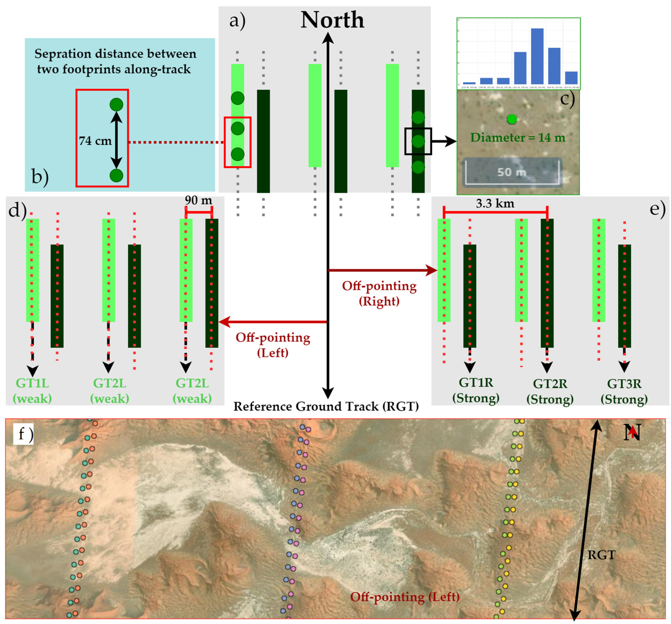
2.1. ATLAS

Onboard ICESat-2, an ATLAS photon-counting lidar (PCL) was placed in a geocentric position close to polar low-altitude Earth Orbit (LEO) at an approximate altitude of 480 kilometers (km) orbiting at the speed of 6.9 km/s with an approximate orbital period of 94.22 min. Unlike most optical satellites, ATLAS operates in ascending and descending modes, collecting data during the day and night. The PCL operation is more favorable during the night to reduce the background noise, and is generally higher during daytime due to background solar radiations [29].

2.1.1. Data Acquisition Mechanisms

ATLAS profiles the Earth’s surface with six laser beams along an imaginary Reference Ground Track (RGT) as shown in Figure 1a. PCL operates at the green wavelength of the visible portion of the electromagnetic spectrum, as PCL technology is mature at 532 nm [28].

ATLAS-PCL operates with a pulse repetition rate (PRR) of 10 kHz that translates into 10,000 laser pulses in one second, illuminating the Earth’s surface with a footprint 14 m in diameter (Figure 1c) [30]. In the along-track direction, two neighboring footprints are separated by 0.74 m spacing (Figure 1b). In total, six laser beams are paired into a weak beam, i.e., 1/4 in power compared to a corresponding strong beam located 90 m apart in the across-track direction (Figure 1d), while each beam pair is 3.3 km apart from the next beam pair (Figure 1e). The notation of Ground Track (GT) with beam numbers (1,2,3) was assigned. To cover more land and vegetation areas along each RGT, ATLAS was off-pointed to the left (L) (Figure 1d) and right (R) (Figure 1e) of the RGT for the first two years of operation; therefore, each beam presents right (R) or left (L) notations, as shown in Figure 1. The example of RGT off-pointing (R) is shown in Figure 1f.

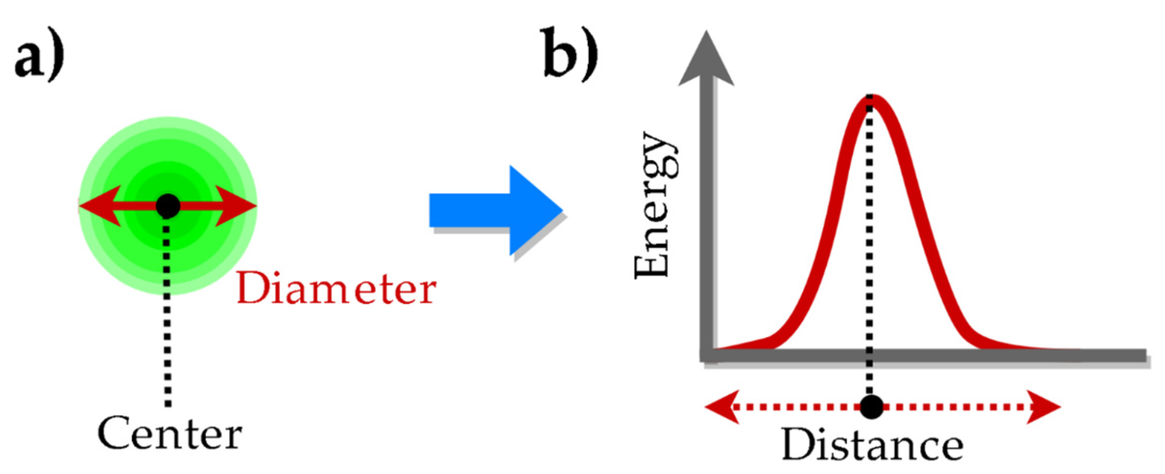
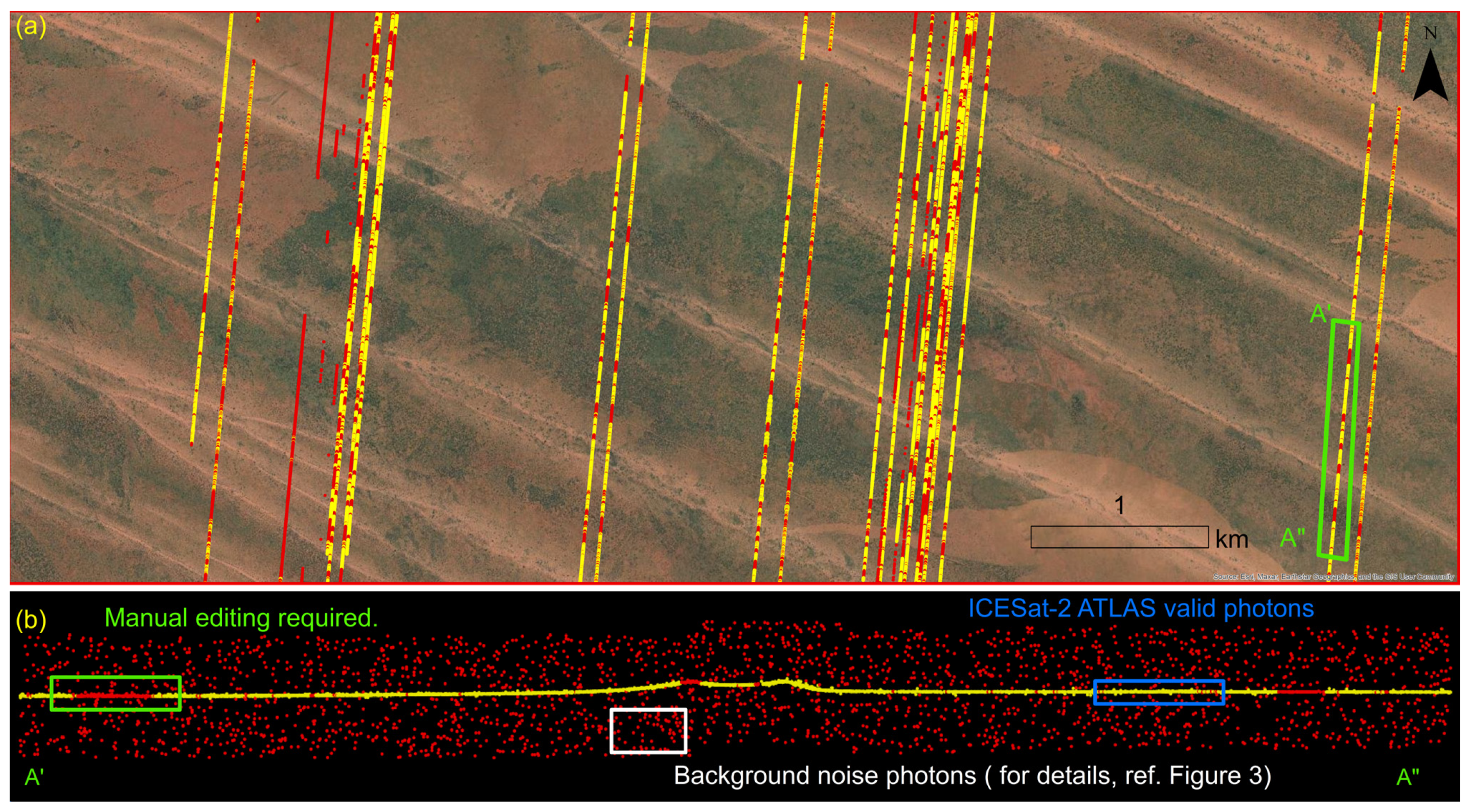
2.1.2. Geolocated Photon Clouds

ATLAS laser-pulse-energy temporal distribution is approximately Gaussian in nature with a circular spot on the ground (Figure 1c and Figure 2). The energy starts decaying from the center of the laser spot towards the edges (Figure 2a).

The ATLAS laser spot corresponding to a strong beam is four times stronger with a pulse energy of 175 micro joules (μJ) than the weak beams with a pulse of 45 μJ. The weak and strong beams are designed by considering the dynamic range of high-reflectance surfaces, e.g., snow, and low-reflectance surfaces, e.g., vegetation, sea, etc. Given the fact that the ATLAS weak beams operate at much lower power levels than strong beams, ATLAS strong beams provide a more complete sampling of low-reflecting terrestrial objects. ATLAS is equipped with a photon-counting LiDAR (PCL) sensor sensitive at the photon level, i.e., a single photon reflected from Earth’s surface at 532 nm wavelengths is registered by the ATLAS sensor. The ATLAS instrument uses photon-counting techniques to measure the Time of Flight (TOF) for a photon to travel from ATLAS to Earth and back to the sensor, and, with altitude (z) above the ellipsoidal reference system [31], ATLAS also precisely records the latitude and longitude of each photon and the collected photon data are referred to as the “geolocated photon cloud”. More details about the ATLAS-PCL sensor can be found at [28]. Single-photon-sensitive LiDAR systems are capable of detecting individual photons backscattered from terrestrial objects, as opposed to linear-mode instruments, e.g., ALS systems that require thousands of backscattered photons in order to detect a return [32]. Nevertheless, ALS systems essentially record strong backscattered pulses from terrestrial objects instead of single photons; therefore, the term “point clouds” is used to describe the number of backscattered laser echoes. For that reason, PCL systems are prone to background-noise photons, e.g., photons generated by sunlight at green wavelengths, i.e., 532 nm, are also registered by PCL systems. In addition, PCL sensors operating at 532 nm are capable of penetrating through water columns; therefore, they are useful for the shallow-water bathymetry of coastal waters and lakes [32,33].

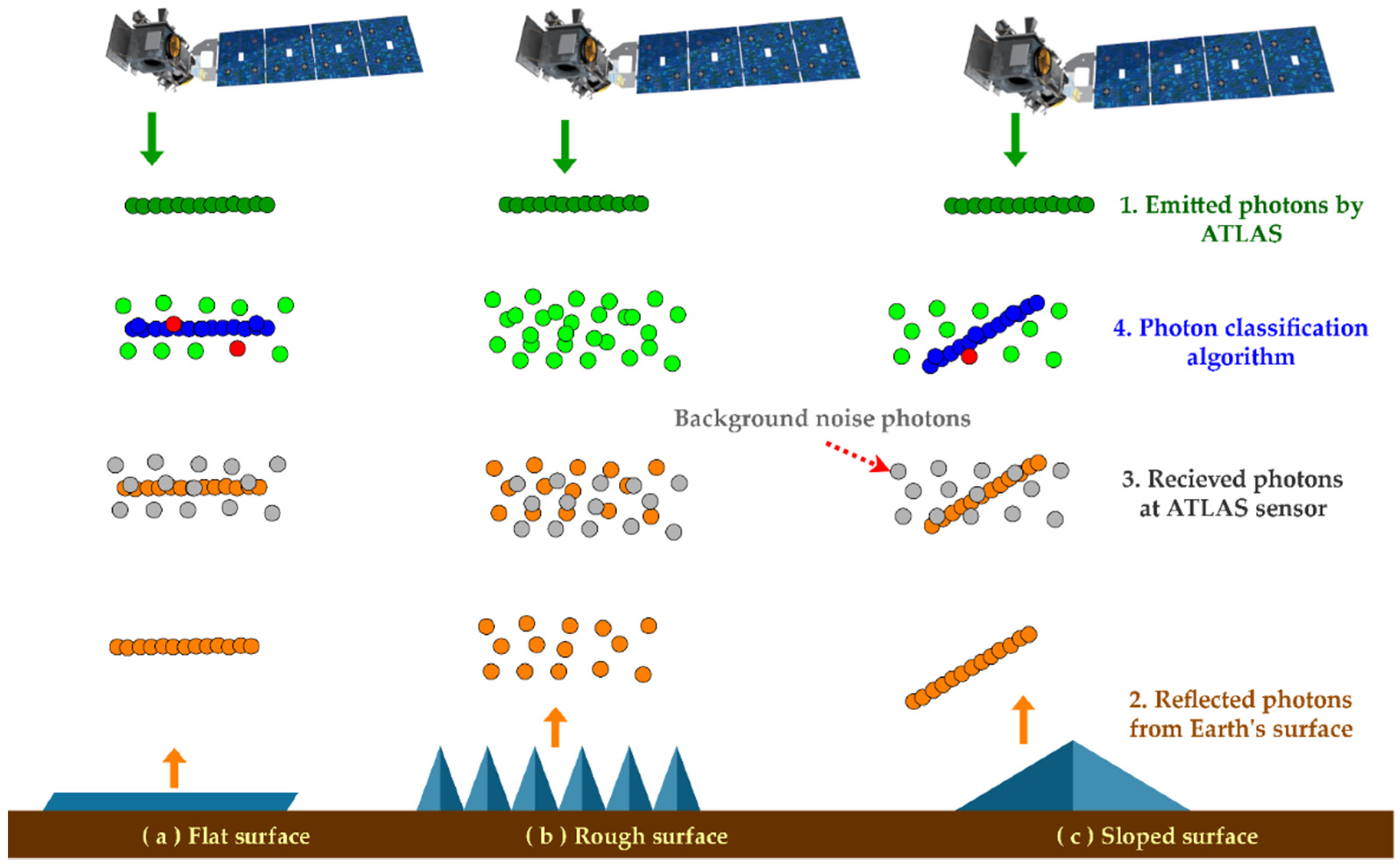
2.1.3. Topographic Effects on Photon Clouds

Topography in the most general form is characterized by three different types: (a) flat, (b) flat-but-rough, and (c) sloped surfaces, as demonstrated in Figure 3. The received photons by the sensor from different surfaces exhibit dissimilar distributions in 3D space and time characterizing the topographic details (Figure 3) [31]. The emitted and corresponding reflected photons received by the sensor show a similar distribution response from flat-but-smooth surfaces (Figure 3a). Over a rough surface of peak and valley configurations, some photons are reflected from the top of the peaks, fewer from the slope surfaces stretching between peaks and valleys, and some are reflected from the valley (troughs), as demonstrated in Figure 3b [31]. For sloped surfaces, the photons from the upper edge of the footprint are received earlier than photons from the lower edge (Figure 3c). In addition, due to the background radiation effect, the photon events recorded by the ATLAS receiver telescope 0.8 m in diameter within the 45 m receiver Field of View (FOV) are comprised of signal and noise photons, respectively. PCL sensors are prone to detect a large portion of noise photons, i.e., originating from the sun and instruments. ATLAS onboard algorithms reduce the size of telemetered data [32] by removing a large portion of noise photons [33,34]. ATLAS onboard algorithms ensure that most of the signal photons within a Range Window (RW) of several hundred meters above and below the onboard reference DEM surface are retained [32]. In addition to this, the ATLAS receiver is equipped with special filters, only permitting photons with wavelength closer to 532 nm, ensuring most of the received photons are signal photons. However, some of the noise photons with wavelengths closer to 532 nm are received by ATLAS sensors (Figure 3, gray dots) [33,34].

Within the RW, ATLAS signal photons reflected from Earth’s surface show a less random distribution (orange dots) than noise photons (gray dots); therefore, the ATL03 algorithm uses the along-track histogram technique to keep only the most likely signal photons. Based on the distribution of the received photons in an along-track histogram, the algorithm automatically assigns the confidence tags to the received photons, e.g., high-confidence- (blue), medium-confidence- (red), and low-confidence-signal photons (green) (Figure 3).

2.1.4. Geophysical corrections

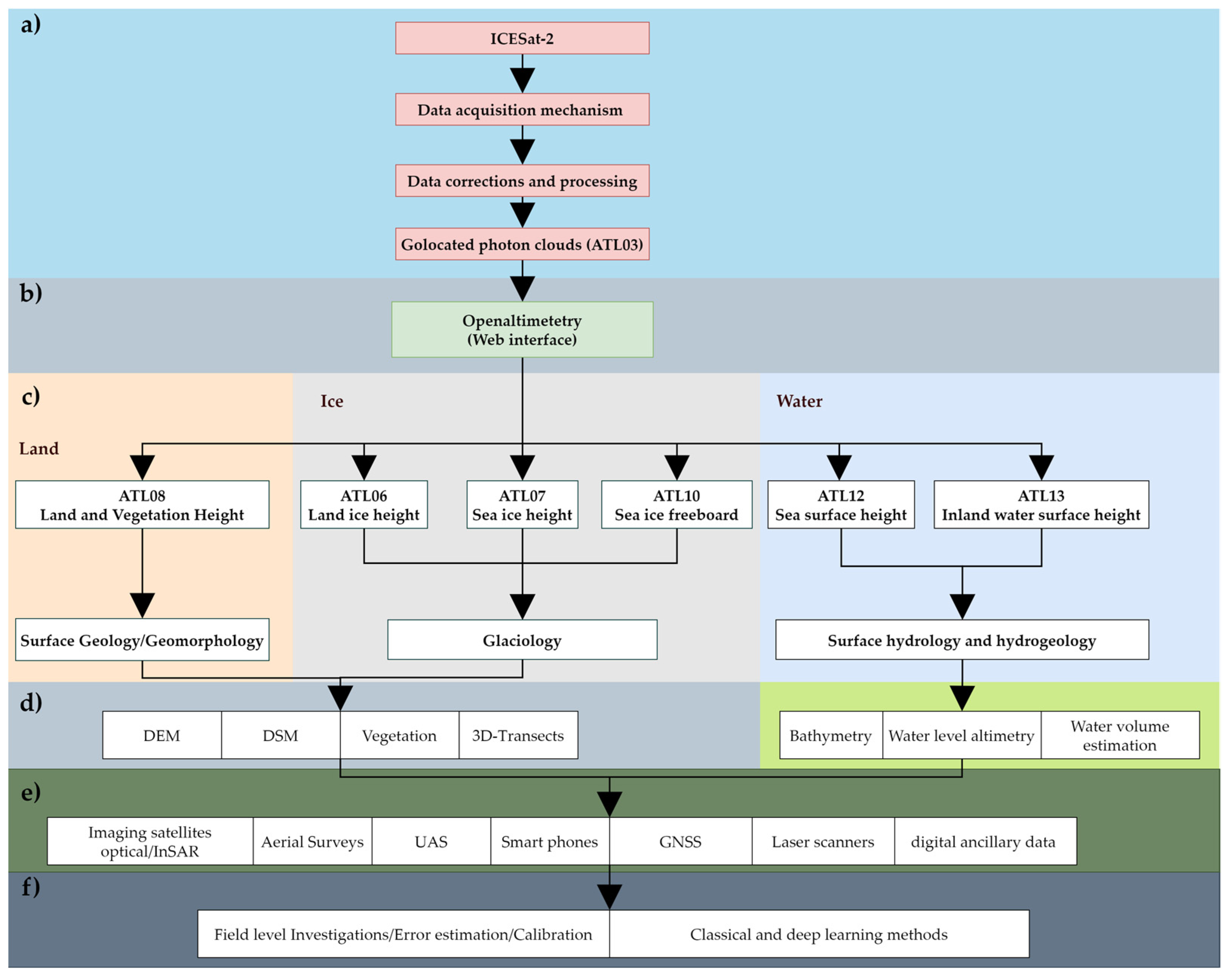
Along with the confidence thresholding of photons (Figure 3), onboard ICESat-2, the ATL03 algorithm also applies geophysical corrections [35] to obtain global geophysical-corrected photon heights based on Equation (1):

$$H_{gc}=H_P-H_o-H_{OL}-H_{DAC}-H_{SEPT}-H_{OPT}-H_{SET}-H_{TCA}$$

(1)

where ${(H}_{gc})$ is the geophysically corrected height of each received photon ($H_P)$ by removing the effects of ocean tides ($H_o$) and ocean-loading tidal effect ($H_{OL})$, which is caused by the elastic response of Earth’s crust to ocean tides, dynamic atmospheric corrections ($H_{DAC}$), solid Earth pole tides ($H_{SEPT}),$ ocean pole tides $(H_{OPT}$), solid Earth tides ($H_{SET}$), and total column atmospheric delay corrections $\left(H_{TCA}\right)$. Therefore, ICESat-2 data products do not require complex geophysical corrections for end users. However, the ATLAS green laser can penetrate through shallow water columns paving the way for bathymetric applications. Water-column-refraction effects are not removed from the photon clouds over water bodies [36]. For space altimetry, the elevation is usually recorded using reference ellipsoid WGS84; therefore, geolocated photons should be corrected for orthometric heights for comparison with other geospatial elevation products, e.g., DSM and DEM.

2.2. Data Products

The ATL03 algorithm generates geolocated photon clouds, i.e., ATL03′s first and most comprehensive data product, which contains the complete set of photons received from terrestrial objects, e.g., ice, vegetation, water, and land, including background noise (Figure 4a,b), with many algorithms available to remove background noise [34,35].

The ATL03 product is further processed by advanced algorithms to produce surface-specific products, e.g., land-ice height (ATL06), sea-ice height (ATL07), land and vegetation height (ATL08), sea-ice freeboard (ATL10), ocean surface height (ATL12), and inland water surface height (ATL13), as shown in Figure 4c. Each product type offers highly accurate geodetic control points important for large applications representing Earth’s surface processes. For example, ATL08 provides highly accurate elevation measurements of bare-Earth (ground) and off-the-terrain (OT) objects (e.g., buildings, vegetation) useful to evaluate the DEM and DSM originating from other sources (e.g., SAR, photogrammetry, satellite imagery) (Figure 4d). For the cryosphere investigation, ATL06 was derived using an ice-extent mask generated using satellite datasets. Similarly, the ATL07 product was specific to sea-ice height studies. In the context of structural geological visualizations and investigations, ATL08 was of more interest because it covers the land and vegetation heights sampled at a 100 m cluster of photon clouds. To ensure data parameter consistency in the ATL08 data product, a fixed step size of 100 m was deliberately selected. This uniform step size guaranteed a consistent canopy (i.e., vegetation) and terrain metrics along the track direction, thereby enhancing the usability of the final products for users. For vegetated areas, the chosen resolution of 100 m typically yielded around 140 signal photons, which were utilized for calculating terrain and canopy height parameters. However, it is worth noting that there may be instances where the number of photons exceeds 140 or falls below that threshold. The heights derived from the ATLAS instrument were defined as the absolute height above the WGS84 ellipsoid. Within each 100 m step of the data, various land parameters were included. These parameters consisted of the mean, minimum, maximum, median, standard deviation, mode, and skewness of the photons classified as ground. Additionally, the data provided the height associated with the interpolated ground line (h_te_interp) at the midpoint of each 100 m segment [19]. Highly accurate ICESat-2 data products are useful to incorporate with aerial imagery, UAS data, smartphones, GNSS, and other digital ancillary data to quantify the error or elevation biases (Figure 4e). For wall-to-wall mapping, ICESat-2 elevation products are useful for machine learning-based regression and classification applications (Figure 4f) [36,37,38].

2.3. Data Access and Processing

The data were available through several options, e.g., the OA web-based cloud platform https://openATLimetry.org/data/icesat2/ (accessed on 16 January 2023), for interactive online Web-based visualization [39], and a comprehensive list of all the derived data products can be found on the National Snow and Ice Data Center (NSIDC) website https://nsidc.org/data/icesat-2/data (accessed on 16 January 2023). In addition, a NASA Earth Data Search provided access to all ICESat-2 data products, along with customization options, e.g., photon clouds within the Area of Interest (AOI) using a shapefile or bounding box.

ICESat-2 data comprised 200+ variables and are mostly available in a Hierarchical Data Format (HDF) for easy storage and retrieval [40]. To process ATLAS data using commercial and open-source software applications, e.g., Python, Java, MATLAB, and R programming, several software applications were developed. A comprehensive list of software applications is available on NSIDC https://nsidc.org/data/icesat-2/tools (accessed on 16 January 2023) and summarized in

Table 1. ICESat-2 data processing software applications based on commercial and open-source platforms.

Name	Platform	Data		Subsetting
		Input	Output	Spatial	Temporal	Variables
Icepyx 1 [41]	Python/notebook	Online	HDF5	Yes	Yes	No
Panoply 2 [42]	Java/GUI	netCDF/HDF/ GRIB	JPEG/PNG/TIF/KMZ/PDF	Yes	Yes	Yes
PhoREAL 3 [43]	Python/GUI	HDF	ASCII/CSV/HDF5/ KML/PNG/LAS	Yes	Yes	Yes
LaRC 4 [40]	Web/GUI	Online	GIF/ASCII	Yes	No	No
IceFlow 5	Python/notebook	Online	HDF/CSV/ASCII	Yes	Yes	Yes
PhotonLabeler 6 [44]	MATLAB/GUI	HDF	LAS/HDF/	Yes	Yes	Yes
IceSat2R 7	R/RStudio	OA API		Yes	Yes	No

¹. https://github.com/icesat2py/icepyx/tree/main (accessed on 16 January 2023); ². https://www.giss.nasa.gov//tools/panoply/ (accessed on 16 January 2023); ³. https://github.com/icesat-2UT/PhoREAL (accessed on 16 January 2023); ⁴. https://cloudsgate2.larc.nasa.gov/cgi-bin/predict/predict.cgi?_ga=2.130658959.1671241382.1673279224-613752272.1672687542 (accessed on 16 January 2023); ⁵. https://github.com/nsidc/NSIDC-Data-Tutorials/tree/main/notebooks/iceflow (accessed on 16 January 2023); ⁶. https://github.com/Oht0nger/PhoLabeler (accessed on 16 January 2023); ⁷. https://github.com/mlampros/IceSat2R (accessed on 16 January 2023).

. Most of the applications ensured certain functions to input the data, such as extracting data within an Area of Interest (AOI), herein referred to as spatial subsetting. Within the AOI, the subsetting further allowed us to download the data within the desired time based on start/end dates or day/night operations. In addition, out of 200+ variables in the ICESat-2 data, only the user’s desired variables, e.g., location coordinates (x, y), elevation above ellipsoid (z), along with photon quality flags (e.g., high, medium, low), could be filtered out within the AOI, herein refer to as variable subsetting to reduce the data size. To consume the processed ICESat-2 data in frequently used mapping software applications, the output is generally provided in the most frequently used data formats, as listed in Table 1.

2.4. Study Areas

To demonstrate the effective use of ICESat-2 data in desert environments, study area A in Oman and study area B in Australia representing aeolian desert environments of star and linear sand dunes were selected as case studies (see Figure 5a). Dunes, the most common form of desert land features, are developed by winds and composed of loose sand particles that are transported by the wind; therefore, they can change, extend, and grow in size and shape, depending on wind energy and direction [45].

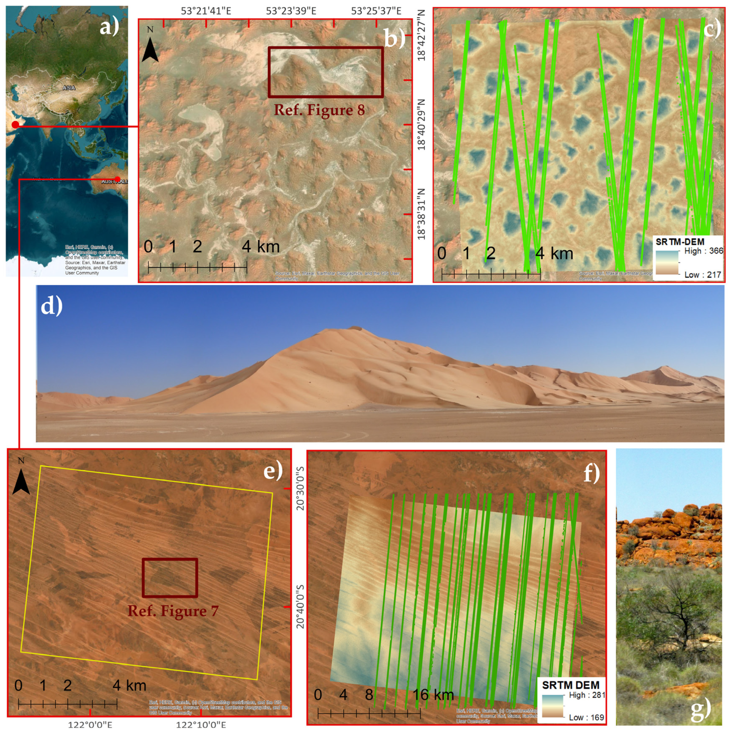
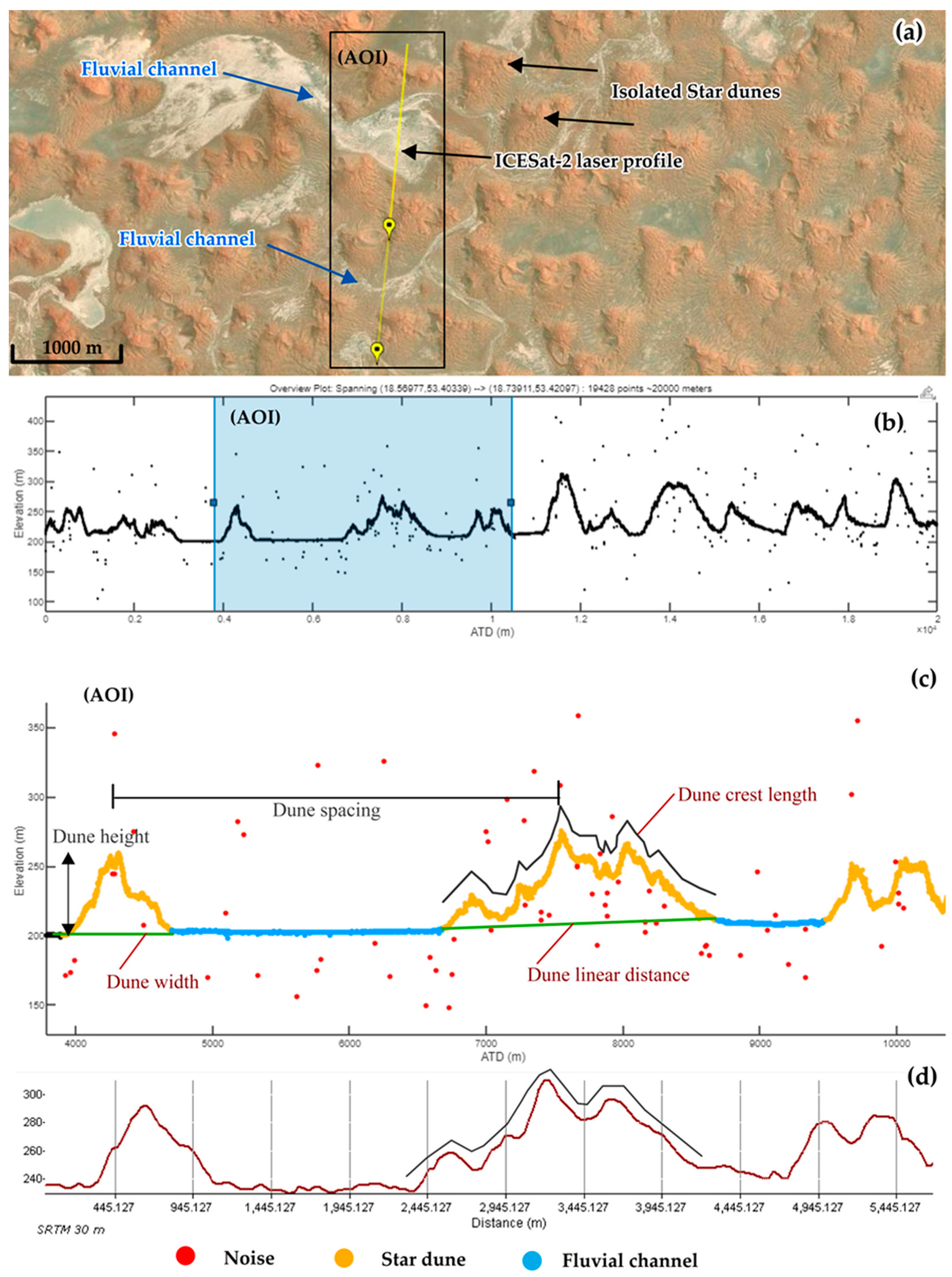
2.4.1. Site A—Star Sand Dunes

Study site A located at geographic coordinates (53°22′51.097″E 18°39′32.313″N) was composed of star sand dunes with fluvial channels and covered a total area of 103.73 km² (see Figure 5b) with HR imagery located in the Rub Al-Khali sand sea in northern Oman [46]. A total of sixty-three star dunes of different sizes were found at site A, as displayed using SRTM 30 m DEM, as shown in Figure 5c, and the terrestrial photo depicts the microtopography of star dunes in Figure 5d.

2.4.2. Site B—Longitudinal Linear Sand Dunes

Site B located at geographic coordinates (122°5′27.751″E 20°37′3.285″S) was composed of linear or longitudinal sand dunes that covered a total area of 1076 km², as shown by HR imagery (Figure 5e), located in the Great Sandy Desert in north-western Australia. Site B covered longitudinal sand dunes oriented in the SE–NW direction, marginally covered with a vegetation type known as “Acacias”, as indicated by the red box in Figure 5e and the terrestrial photo in Figure 5g. The majority of the described Acacia species (≈1300) in Australia are in the subgenus Phyllodineae. Phyllodinous acacias exhibit heteroblasty, i.e., they show distinct juvenile and adult leaf forms and, therefore, exhibit great geometrical and structural diversity at different growth stages [47]. A visual estimation revealed that there were about eighty-seven longitudinal sand dunes at site B. The geometrical depiction of longitudinal linear sand dunes is shown in Figure 5c using SRTM 30 m DEM.

2.5. Data Processing and Methods

The ICESat-2 ATL03 product (Figure 4a) was downloaded (e.g., green lines in Figure 5c,f) with spatial subsetting for study sites A and B using NASA Earth Data Search application: https://search.earthdata.nasa.gov/search (accessed on 16 January 2023). In addition, two other datasets, e.g., ASTER and Advanced Land-Observing Satellite (ALOS)/Phased Array-Type L-band Synthetic Aperture Radar (PALSAR) DEMs were also acquired using the NASA Earth Search Application for sites A and B [48]. The acquired datasets, along with their documented global accuracies in root mean square error (RMSE), are listed in

Table 2. Summary of acquired datasets for two study sites.

Product Name	Resolution (m)	Elevation RMSE (m)	Ref.
SRTM	30	≈14.00	[49]
ASTER	30	≈08.40	[49]
ALOS-PALSAR	12.5	≈04.00	[49]
ICESat-2 ATL03	14 m (footprint)	≈00.48	[50]

.

The acquired datasets (Table 2) were processed using several software applications documented in Table 1. Global DEM products, e.g., SRTM, ASTER, and ALOS-PALSAR, were processed using ArcGIS Desktop 10.8 (ESRI, Redlands, CA, USA), and ICESat-2 ATL03 was first processed using the PhoREAL software application [44] to convert HDF [51] data into a point-cloud LAS format [52]. In addition, LAS data were processed using the modern Hierarchical Density-Based Spatial Clustering of Applications with Noise (HDBSCAN) Python package to remove background-noise photons (see Section 2.1.2 and Section 2.1.3) from the data, as shown in Figure 6a,b [53]. We objectively demonstrated the use of the software applications documented in Table 1 in order to download, pre-process, process, and classify ICESat-2 data products.

In addition, all datasets were projected to the Universal Transverse Mercator (UTM) World Geodetic System (WGS) 84. Global DEMs were normalized where the lowest elevations were set to zero to obtain consistent height metrics. Similarly, following noise removal, ICESat-2 point clouds were normalized, whereas the lowest elevation points were set to zero [54]. The evaluation of global DEM products compared with ICESat-2 ATL03 was performed using RMSE and Mean Absolute Error (MAE), while linear regressions were performed to find the correlation (R²) between ICESat-2 and global DEM products [55].

3. Results

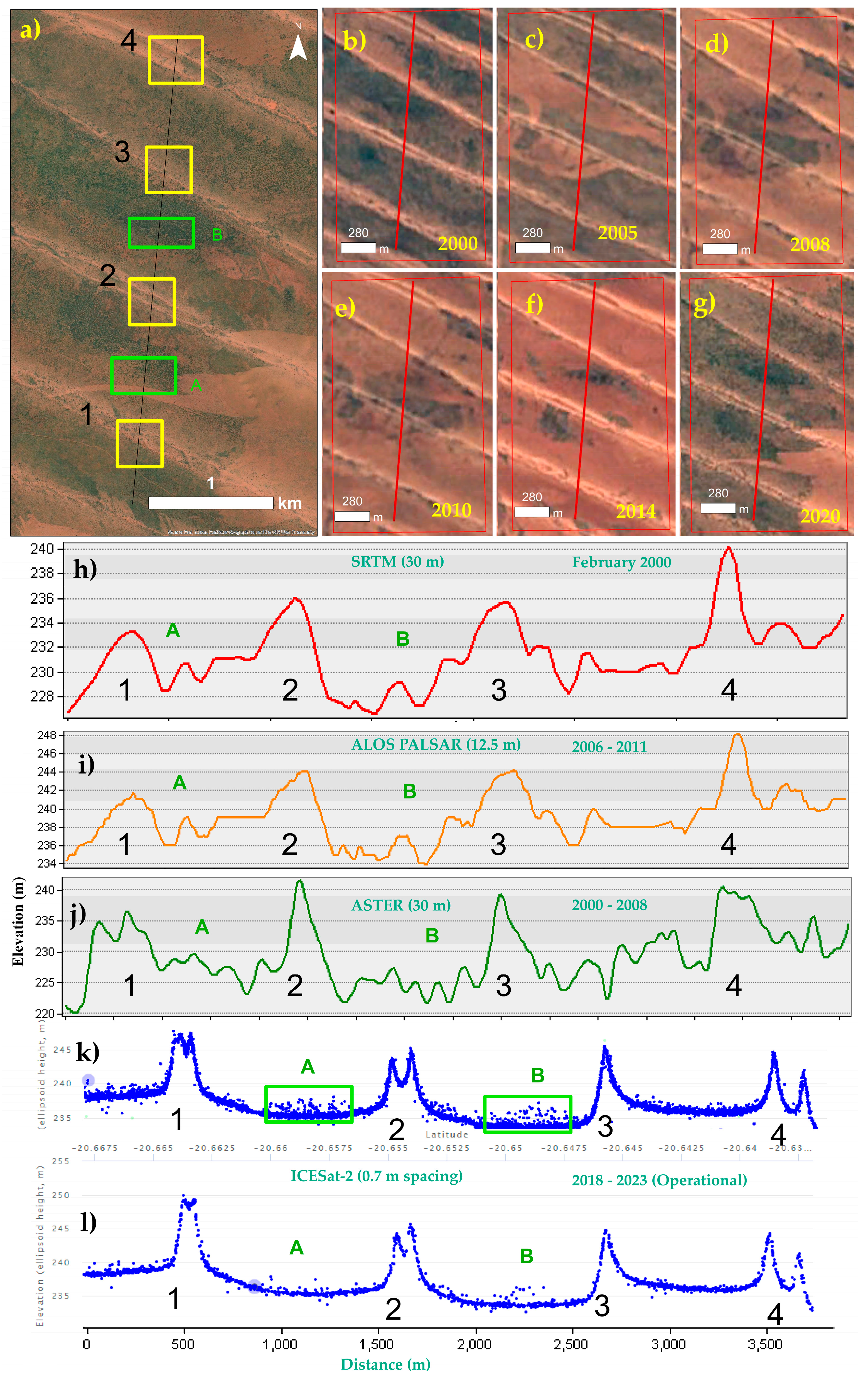
3.1. Comparison with Global DEM Products

Geological Education and Investigations

Desert-margin settings are composed of fluvial and aeolian processes that rarely operate individually and usually work on feedback mechanisms from each other, i.e., fluvial processes are governed by aeolian processes and vice versa. Nonetheless, changes in aeolian processes alter the fluvial processes that, in response, trigger further changes in aeolian processes until a balance is achieved [56]. The present study was designed to present sand dune structures, purely from the ICESat-2 data standpoint; therefore, a detailed description of these features can be found in [31].

In the context of the geological education and investigations of an Area of Interest (AOI), optical imagery provides the wall-to-wall mapping of AOI composed of different geological features, e.g., channels, dunes, and vegetation, with two-dimensional (2D) spaces (Figure 7a). A more comprehensive analysis aims at using the spectral responses of different cover types, e.g., sand, soil-crust, vegetation, and salinity indices, using medium-resolution satellite images, e.g., Landsat [14,56]. It was found to be challenging to discriminate between sand dunes and sand sheets exclusively based on the spectral data, since both are composed of sand deposits and show homogeneity in the image spectra (Figure 7b–g) [14]. To discriminate between and decipher the differences in their shape and sizes, DEM or DSM (e.g., SRTM) are usually draped over the optical imagery to show the geometrical characteristics of different terrestrial objects for geological investigations or geological education purposes in a classroom environment. A frequently used approach is to construct 3D transects to decipher the structural construct of different terrestrial objects, e.g., sand dunes, as shown in Figure 7h–j, using SRTM, ALOS-PALSAR, and ASTER DEM products, respectively. The DEM draping technique is useful for visualizing geometrical characteristics; however, it is constrained by several factors. First, high-resolution (HR) satellite imagery is available commercially at a nominal price or freely through Google Earth (GE) Pro [57], globally, which is frequently updated and offers a new geological resource for mapping, e.g., Figure 7a [58]. On the contrary, global HR-DEMs produced by commercial/government agencies are cost-prohibitive/restrictive, consequently, they are ousted by freely available mediums or coarse-resolution DEMs, e.g., SRTM (Figure 7h) [15,59]. Unlike satellite imagery, global DEMs are based on single-mission (e.g., SRTM) data with little or no temporal resolutions; therefore, geometrical changes in the Earth’s surface posterior to DEM production are absent [60]. ICESat-2, therefore, helps us to understand and quantify such changes with much higher spatial–temporal resolutions (for details, see Section 3.5) [20]. Figure 7 shows that the ICESat-2 data are robust in depicting the aeolian dunes, deciphering the dunes’ widths and heights in much greater detail (Figure 7k,l) compared to SRTM (30 m), ALOS-POLSAR (12.5 m) [61], and ASTER (30 m) DEMs products (Figure 7h–j) [42].

Furthermore, global DEM datasets were collected between 2000–2011 [43]; in the past two decades or so, the surface geological realm has significantly altered under the influence of erosion and deposition (Figure 7b–g), thus making global DEM products outdated for many regions in the world [44], including desert environments (Figure 7). Owing to their medium resolution at 30 m DEM, e.g., SRTM or ASTER, and the influence of interpolation methods to obtain a gridded DEM, textural and surficial information is lost (Figure 7h–j).

According to Shumack et al., 2020, vegetated linear dunes in the Simpson Desert in Australia are low in height (>10 m), as revealed by ground surveys; therefore, linear sand dunes are generally not well presented by ASTER and SRTM DEM products, given the fact that medium-resolution DEM products with 30 m GSD showed under and over estimations of terrain elevations (z); the documented global RMSE values are shown in Table 2 [45]. Therefore, ICESat-2 offers the unique opportunity to derive and quantify the planimetric dune patterns at a much higher resolution, which was not possible in the previous studies (Figure 7). Figure 7 also indicates that global DEM products depend on onboard sensors for data collection. For example, 3D-elevation transects show similar elevation patterns for SRTM and ALOS-PALSAR DEMs (Figure 7h,i) [61] compared with ASTER-DEM derived from stereo-imagery (Figure 7j) [20]. In addition, given the fact that the data were collected at different periods, the planimetric dune patterns derived using global DEMs were more likely to yield inconsistencies (Figure 7h–j). On the contrary, ICESat-2 data (Figure 7k,l) were more consistent with HR imagery (Figure 7a) with exact data acquisition time tags. The temporal aspects of ICESat-2 are further discussed in Section 3.3.

3.2. Classification and Field Mapping

To segregate and label the photon clouds into different terrestrial objects, e.g., canopy, water, and bare Earth, manual or automated classifications were required [62]. ATLAS photons were unclassified in the ATL03 data product, i.e., no prior information was available for terrestrial objects depicted by photon clouds (Figure 8b). Analogous to labeling over satellite imagery, to segregate the photons into their respective features, e.g., terrestrial objects, photon labeling was required, as shown in Figure 8c [44]. We used PhotonLabeler developed by MATLAB (Table 1) [44] with user-friendly GUI to classify raw photon clouds into different classes, e.g., noise, fluvial channels, and star dunes (Figure 8c).

The labeled ICESat-2 photon clouds were useful to derive planimetric dune patterns metrics, such as dune crest length, i.e., the horizontal length of the dune crest line (Figure 8c); dune crest density, i.e., total number or length of dune crest lines per counting unit; dune sinuosity, i.e., the crest length divided by the linear distance between dune termination; dune spacing, i.e., the crest-to-crest distance between dune crests or dune wavelength; and dune width and height (see Figure 8c). The present study only considered dune height metrics as a showcase study (for details, see Section 3.4). Compared with HR satellite imagery (Figure 8a), a quantitative analysis of planimetric dune pattern metrics is limited without high-resolution LiDAR data, e.g., HR-DEM [63]. To this end, ICESat-2 fills this gap to some extent (see Figure 8c). Compared with ICESat-2, global DEM-based planimetric dune pattern metrics, e.g., dune crest length, sinuosity, and dune height, are outdated, with elevation errors that need to be quantified (see Figure 7h–j and Figure 8d). Figure 8c indicates that star dunes depict more complex sinuosity using ICESat-2 data than SRTM-DEM (Figure 8d). Compared with terrestrial photos (Figure 5d), ICESat-2 can decipher the star dunes’ microtopography that was lacking in global DEM products (Figure 8c,d).

In the context of field mapping, the collection of Ground Control Points (GCPs) through GNSS field surveys is an essential step to assess and quantify the accuracy of global DEM products, e.g., SRTM DEM (for details, see Section 3.3). The accuracy evaluation is crucial for concluding the suitability of different DEM products. However, collecting GCPs, referred to as “field mapping,” is expensive and labor-intensive, particularly in desert regions. To this end, ICESat-2 time-tagged photon clouds offered an extensive profiling of large areas, significantly reducing the field mapping tasks (see Figure 8c). Moreover, ICESat-2 photon clouds enabled the direct acquisition of GCPs of inaccessible regions, such as dune peaks, which were difficult to access due to loose sand [15]. In addition, extensive GCPs profiling compared with ICESat-2 seems challenging for time-constraint projects [16].

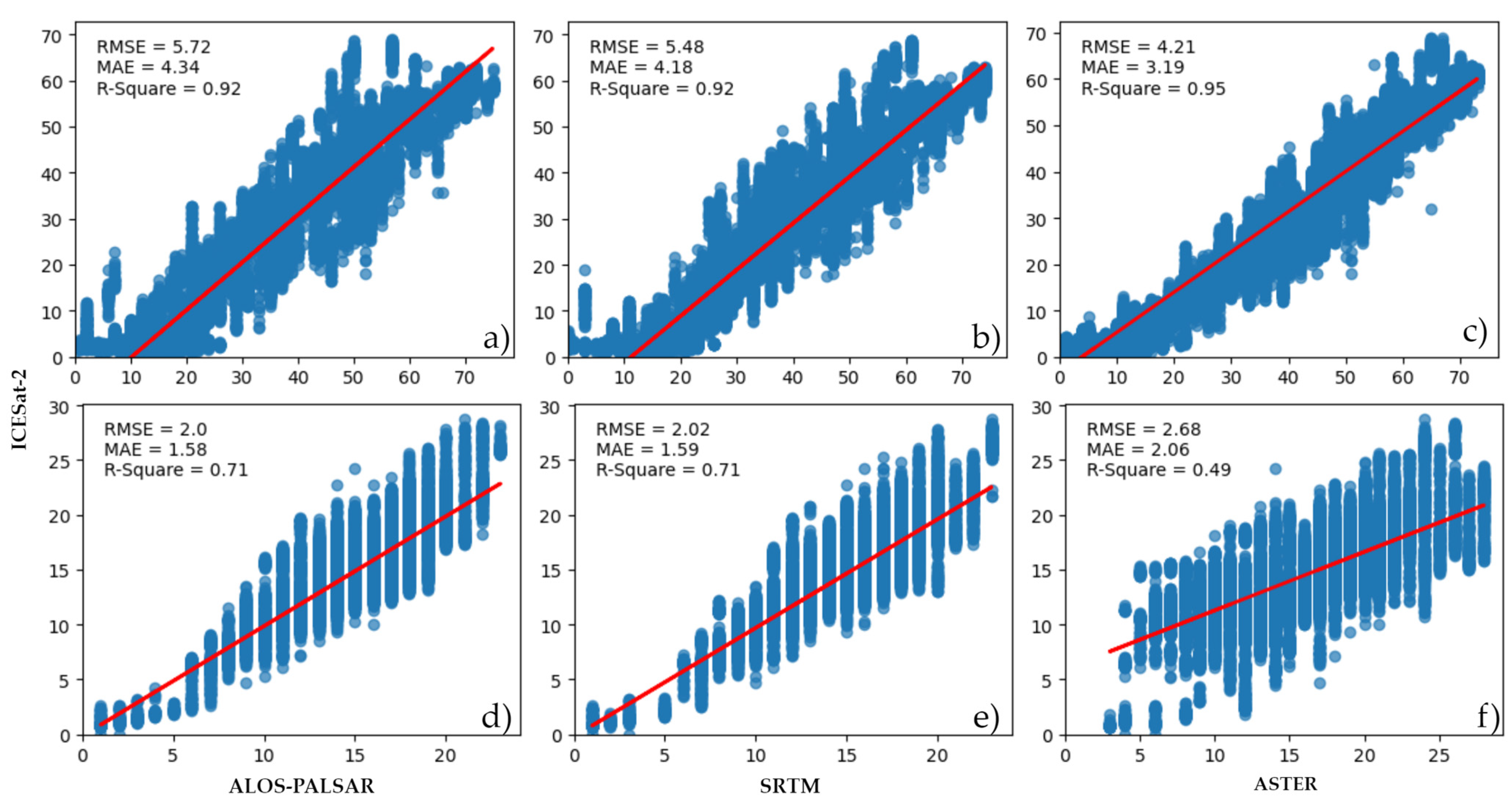
3.3. Elevation (z) Accuracy Assessment

Accuracy evaluation of DEMs is an important step in establishing the metrics obtained from elevation, e.g., sand dune height [49]. Traditionally, this is accomplished by collecting sparse elevation points through GNSS field surveys or LiDAR measurements [63]. A common method for assessing accuracy involves calculating RMSE, MAE, and R² values, which allow for the quantification of error budgets and correlations between the DEMs and reference data, e.g., GNSS.

In this study, ALOS-PALSAR, SRTM, and ASTER DEMs were evaluated in two sand dune environments (Table 2 and Figure 5) using the quantification metrics of RMSE, MAE, and R², respectively. For site A, ALOS-PALSAR has an RMSE of 5.72 and MAE of 4.34 (Figure 9a), while for site B, the RMSE and MAE values are significantly lower at 2.0 and 1.58 (Figure 9d), respectively. Similarly, the SRTM dataset presents a similar performance for both sites, with RMSE and MAE values of 5.48 and 4.18 for site A (Figure 9b) and 2.02 and 1.59 for site B (Figure 9e). The RMSE, MAE, and R² values are consistent for SRTM and ALOS-POLSAR at both study sites (Figure 9a,b,d,e), with the possible reason that both DEMs are based on active remote sensing, i.e., SAR interferometry techniques [64,65]. Compared with ALOS-PALSAR and SRTM DEMs, ASTER-DEM performed differently between the two sites, with lower RMSE and MAE values for site A, i.e., 4.21 and 3.19 (Figure 9a–c), and higher values for site B, i.e., 2.68 and 2.06 (Figure 9c,f), respectively. Such differences were highly likely caused by ASTER-DEM data sources and production methods, due to the fact that the ASTER-DEM originates from optical satellite imagery through Structure from Motion (SfM), e.g., Ames Stereo Pipeline (ASP), with possible artifacts at an elevation (z) caused by weather conditions, cloud cover, image saturation, and shadows [66]. Moreover, the R² values were inconsistent for both sites across all three datasets, with values ranging from 0.49 to 0.95. The lower R² values for site B can be attributed to the presence of vegetation frictional cover (see Figure 5g and Figure 7a–g).

Nevertheless, as shown in Figure 9, the accurate evaluation of DEMs varied across the two study sites, with site B generally exhibiting lower error values. The lower RMSE and MAE at site B can be attributed to the linear sand dunes, which are more simplified than star dunes (ref. Figure 7k,l and Figure 8c). Figure 9 indicates that ICESat-2 is useful to quantify the elevation (z) inaccuracies of global DEM products, as LiDAR-based methods are more appropriate for accuracy evaluation and assessment [67].

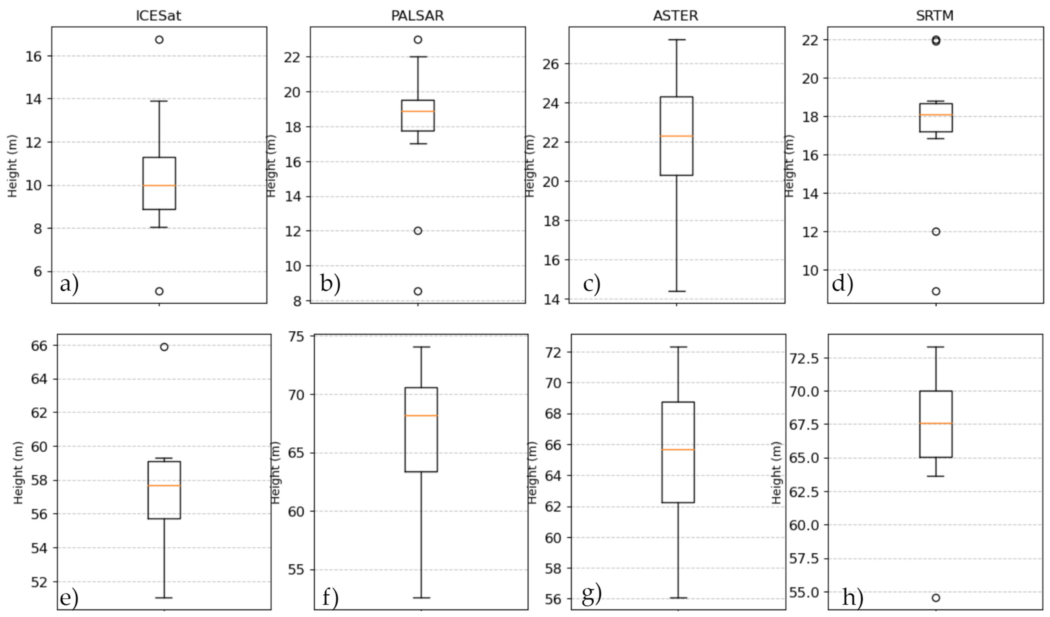
3.4. Dune Height Statistical Analysis

The statistical analysis of dune height was performed to quantify ICESat-2′s performance compared with global DEMs, i.e., ALOS-PALSAR, SRTM, and ASTER products (

Table 3. Statistical analysis of star and longitudinal sand dunes’ heights.

Study Site	Metric	Sensor		Statistical Analysis
			No. of Obs.	Minimum	Maximum	Mean	Std. Dev.
Site A: star dunes	Dune height [45]	ALOS-PALSAR	100	52.6	74.08	66.09	7.30
		SRTM		54.58	73.32	66.51	6.21
		ASTER		56.10	72.34	65.15	5.81
		ICESat-2		51.06	65.89	57.75	4.58
Site B: linear dunes		ALOS-PALSAR	870	8.56	23.06	17.94	4.04
		SRTM		8.93	22.01	17.42	3.67
		ASTER		14.43	27.22	21.84	3.68
		ICESat-2		5.09	13.91	9.92	2.39

). Dune height is a more relevant metric compared with dune spacing and width, which can be measured using high-resolution satellite imagery [57]. The statistical analysis included the minimum, maximum, mean, and standard deviation of the dune heights at sites A and B. The number of star dunes acquired by the ATLAS sensor was about (≈45/63), from which 10 star dunes from site A were selected and each dune was sampled at 10 different, random locations to perform a statistical analysis, which yielded a total (10 × 10 = 100) dune height observation for star dunes. While linear sand dunes covered more ICESat-2 footprints, metrics were performed at 10 random locations of 87 linear sand dunes, given the fact that, unlike star dunes’ longitudinal values, linear sand dunes were consistent linear features for hundreds of kilometers, which yielded more (≈870) dune height observations for site B [46]. The statistical analysis of sand dune heights is presented in Table 3.

Table 3 shows that global DEMs, e.g., ALOS-PALSAR, SRTM, and ASTER, overestimate the dune heights at both study sites (Figure 5 and Table 3). In terms of the resolution, SRTM and ASTER at 30 m showed similar mean and standard deviation values for sites A and B. On the contrary, ALOS-PALSAR at 12.5 m showed the highest standard deviations for both study areas. Table 3 and Figure 10a,e show that ICESat-2 shows more consistent results in both study sites, providing the lowest minimum, maximum, mean, and standard deviation values. ASTER showed great inconsistencies (Figure 10c,g), producing the greatest variability in dune height. Alternatively, ALOS-PALSAR (Figure 10b,f) and SRTM (Figure 10d,e) showed similar performances at both study sites. In terms of the sensors, there were notable differences in the minimum and maximum values for each sensor, indicating variations in the elevations (z) of collected datasets (Table 3). This study, therefore, highlighted the usefulness of ICESat-2 in sand dune studies to quantify the accuracies of global DEM products. Though ICESat-2 is a profiling system and wall-to-wall mapping is not possible, regression techniques are a useful alternative to improve the dune metrics derived from global DEMs or improve the accuracy/resolution of global DEMs [44,65,67].

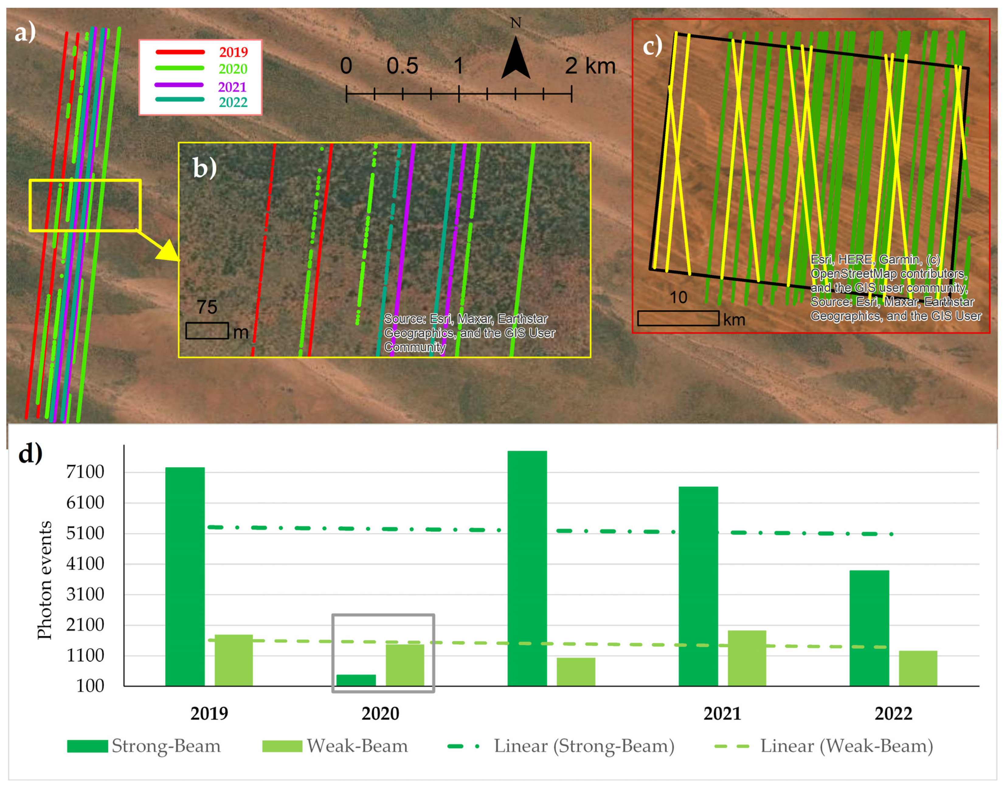
3.5. Temporal Coverage

The high cost associated with multi-temporal ALS-LiDAR data acquisition and processing over a large area is prohibitive. To this end, there is an element of incompatibility of multi-temporal ALS-LiDAR data arising from varying acquisition parameters, e.g., footprint size, wavelength, scan pattern, and beam divergence [12,16]. To quantify the geological changes over a vast area is therefore challenging using ALS, due to data availability and compatibilities issues [16]. On the other hand, traditional global DEMs (e.g., ASTER or SRTM) have fewer revisit times for obtaining terrain spatial–temporal signatures (Figure 7). Legacy digital photogrammetry and LiDAR data are rare at the global scale for time-series assessments of sand dune changes [68]. On the contrary, time-tag photons provide an unprecedented data source (Figure 11d) to quantify volumetric changes in desert environments with documented success for water level changes [69].

The temporal resolution of ICESat-2 cannot be presented similar to traditional satellite missions (e.g., Landsat), given the fact that ICESat-2 operates along imaginary RGT lines with capabilities of off-pointing to the left and right of RGT (see Figure 1). The temporal coverage, including future visits, is shown in Figure 11 for study site B, Australia. Figure 11a shows that, within a distance segment of 500 m east–west, the aeolian sand dunes were visited once every year from 2019 to 2022, except for the year 2020, when the revisit time was doubled. According to the NASA ICESat-2 official web-page (https://icesat-2.gsfc.nasa.gov/science/specs (accessed on 16 February 2023)), ICESat-2 was on safe hold from 26 June to 9 July 2019, and 4 to 12 April 2022. Additionally, the official webpage provided the RGT data for specific dates when ICESat-2 has passed and will overpass a location in the future. The planned RGT for study site B is shown for late 2022 and 2023 (yellow lines in Figure 11c). For a specific Area of Interest (AOI), the Langley Research Center (LaRC) application can be used to determine the ICESat-2 overpass time (Table 1) [40].

In addition, Figure 11d indicates that, with each passing year, fewer photon events were recorded, indicating the aging of the laser system onboard the ICESat-2 ATLAS sensor, along with the effects of environmental conditions [70]. It is worth mentioning that ICESat-2 temporal resolution was constrained by several factors. First, the cloud cover can conceal underlying topographies, thereby creating data gaps (Figure 11d, gray bounding box). Secondly, ATLAS off-pointing capability to cover a larger area along the left and right sides of each RGT ensured that some locations were frequently visited, especially the middle beams, as compared to the edge beams within the sensor footprint (Figure 11b). For site A, Oman, the ICESat-2 covered forty-five star dunes out of a total of sixty-three that were mapped using HR imagery and SRTM-DEM, which shows that, within an area of 10 km by 10 km, ICESat-2 covered 71.42% star dune fields at a high resolution (Figure 5c).

4. Discussion

The potential of providing field-level structural details of fluvial and aeolian processes using time-tagged ICESat-2 photon returns was assessed. Finally, how weak and strong beams interact with these features presents the complex micro-topography using difficult to obtain from traditional DEM-based height transects (see Figure 7 and Figure 8). A LiDAR signal can penetrate through canopies; the ICESat-2 3D transect reflects surface characteristics, e.g., surface roughness, presence, or absence of canopies with the exact date and time compared to global DEM products (see Figure 7). ICESat-2 provides very high-resolution elevation transects deciphering the dunes, channels, channel width, dune height, and vegetation within the channel using ATLAS strong (Figure 7k) and weak beams (Figure 7l). On the contrary, global DEM products’ 3D-elevation transects showed outdated channels and dunes, while surficial features were completely absent from the data (Figure 7h–j).

In the context of geological education in a classroom environment, ICESat-2 3D-elevation transects revealed robust information about the structure of sand dune features, e.g., peaks, valleys, and vegetation present within the valleys (see Figure 7k,l), compared with global DEM products (Figure 7h–j). ICESat-2 data products through OA [39] can interactively be visualized through a Web platform with a stable Internet connection: https://openATLimetry.org/data/icesat2/ (accessed on 21 April 2023). This certainly offered many advantages over traditional DEM draping over satellite imagery techniques (Figure 5). Geologists are more interested in the elevation transects of different lithological groups interpreted from high-resolution satellite imagery (Figure 7a). OA provided a single platform with the integrated use of recently acquired high-resolution satellite imagery (Figure 7a), with ICESat-2 and level-2 -3 products, e.g., ATL06 (land-ice height), ATL07 (sea-ice height), ATL08 (land and vegetation heights), ATL10 (sea-ice freeboard), ATL12 (ocean surface height), and ATL13 (inland surface water height), as shown in Figure 4. OA also provided several interactive GIS functions via a Web-based GIS platform traditionally implemented in most spatial data processing software packages, e.g., QGIS, ArcGIS (ESRI, Redland, CA), etc. Additionally, ICESat-2 GLT could be accessed by data acquisition dates. Furthermore, OA offered a search by location functionally, or zoomed into the AOI based on the provided coordinates, e.g., city or country name based on the location database of NASA. OA provided excellent ease of use with ICESat-2 data visualization, globally. However, OA does not work on tablets and smartphones without Internet access. To address this challenge, ICESat-2 photon clouds can be downloaded in a CSV format for use by other offline platforms, such as QGIS, etc. Detailed documentation regarding OA design philosophy can be found in the developer information [40].

In the context of field mapping, the ICESat-2 photon returns from different lithological groups, which significantly facilitate the preparation of digital procedures, including laboratory pre-fieldwork, survey fieldwork, and the interpretation of post-fieldwork. For example, the acquired Ground Control Points (GCPs) using GNSS can be plotted to evaluate the accuracy of ICESat-2 data and vice versa (Figure 9 and Figure 10) [26]. Therefore, for inaccessible regions, ICESat-2 data can be used directly to reduce overall field-mapping tasks (Figure 7k,l) [15]. The application spectrum of ICESat-2 data is wide-ranging, producing global- to local-scale planimetric dune patterns, as shown in this study (Figure 10 and Table 3). For example, Ground Control Points (GCPs) and Control Points (CPs) are important datasets generally acquired using highly accurate GPS/GNSS observations to quantify the accuracy of DEM/DSM originating through photogrammetry techniques using satellites, aerial, or UAS surveys [43,50]. Nevertheless, highly accurate geodetic-level ICESat-2 observations provide an alternative to traditional GPS/GNSS-based field surveys. Unlike traditional ALS data, ICESat-2 temporal coverage enables the 3D volumetric-change-detection application at a global scale (Figure 11).

The present study only discussed the application potential of ICESat-2 data in desert environments by studying star and linear sand dunes, in order to introduce a benchmark for in-depth studies. To this end, we evaluated the usefulness of ICESat-2 compared to global DEM products. First, we quantified the overall accuracies of global DEM products (Figure 8) and then dune height metrics were assessed (Figure 10 and Table 3).

The study of arid dune field vegetation, i.e., photosynthetic vegetation ($f_{PV}$) and non-photosynthetic vegetation ($f_{NPV}$), was important to understand the arid ecosystem dynamics (Figure 7b–g) of vegetation species, e.g., Acacias. The studies indicated that medium-resolution satellite imagery, e.g., Landsat (30 m) or Sentinel-2 (10 m), was been extensively used to understand arid ecosystem dynamics [71]. However, vegetation functional traits (e.g., plant height and crown area) are possible to obtain, at present, using ICESat-2 data, as shown in the green box in Figure 7k,l. However, ICESat-2 strong beams (Figure 7k) revealed further information about vertical vegetation structure compared with the weak beam (Figure 7l); therefore, I was more useful than weak beams. The accuracy evaluation revealed that global DEMs show significant differences in vertical accuracies; therefore, documented global accuracies were less reliable (Table 2) to quantify the errors for different geographical locations in the world. To this end, ICESat-2 showed consistent and more accurate vertical accuracies useful to quantify the vertical accuracies of global DEMs at local scales (Table 3 and Figure 10).

A longstanding goal of aeolian research is to diversify dune types and their classification using remotely sensed datasets [27,46]. Global DEM products were utilized to identify diverse dune types at 30 to 90 m medium-to-coarse-resolution products (Figure 7 and Figure 8) [14]. ICESat-2 high-resolution LiDAR transects were capable of deciphering dune geometries with richer details, expanding the research scope of dune types and sub-type classifications and mapping (Figure 7k,l and Figure 8).

5. Conclusions

Earth observation from space has enabled repeated scientific investigations at a global scale. The legacy of satellite data has significantly enabled scientists to quantify the growth and development of scientific knowledge using freely available DEM and HR-satellite imagery. To this end, the majority of research investigations have been conducted in a wide-area capacity, including remote regions in desert environments. Aeolian sand dune regions compose the dominant part of the world’s desert regions and are extensively explored and investigated using global remote sensing freely available datasets. Global DEM products have proven to be very effective datasets to quantify the growth and development of aeolian sand dune environments, yet their medium resolution (e.g., 30 m) presented limitations for newly developed, young sand dunes along with sand dunes of a smaller size < 30 m. To overcome the challenges presented by global DEM products, HR-DEM originated from LiDAR datasets proved to be the most effective source of information. Nevertheless, expensive aerial LiDAR surveys are rare in desert environments; therefore, there is a lack of high-resolution LiDAR data products covering global desert environments.

On the other hand, global space-borne LiDAR missions, e.g., ICESat-1 and ICESat-2, provided global LiDAR data with revisit capabilities to address this gap in the research, to some extent. However, the evaluation and quantification of ICESat-2 data in aeolian sand dune environments were lacking in the previous research. The present study showcased the usefulness of ICESat-2 LiDAR data for the case study in two diverse sand dune environments, including star dunes in the Rub Al-Khali desert of Oman and linear longitudinal sand dunes in the marginally vegetated Great Sandy Desert in north-western Australia. The evaluation showed that globally documented RMSE errors of global DEM products, e.g., SRTM, ALOS-PALSAR, and ASTER, were inconsistent in both study areas, which could be quantified using ICESat-2 photon cloud data as a reference benchmark dataset. Similarly, dune height metrics derived using global DEM products also showed inconsistent results compared with ICESat-2 data. The present study is the first of its kind to document the usefulness of ICESat-2 LiDAR data for geological education and in-depth investigations, compared with traditional DEM-based approaches. The goal of aeolian sand dune research is to expand the classification of dune types using remote sensing data. Global DEM products were used to identify various dune types at medium (30 m) to coarse (90 m) resolutions. However, high-resolution LiDAR transects from ICESat-2 provided more detailed and comprehensive dune geometries, opening-up new prospects for studying, mapping, and classifying different dune types and sub-types at unprecedented higher spatiotemporal resolutions never before achieved in previous studies. In addition, ICESat-2 has shown the potential to map and quantify the geometrical traits (e.g., height) of desert vegetation, such as “Acacias”.

However, space-borne LiDAR is a profiling system, and wall-to-wall mapping is not possible when using spaceborne LiDAR alone; therefore, advanced regression and machine learning models can be developed/deployed to integrate global HR imagery and medium-resolution DEM products with ICESat-2 data to further improve aeolian sand dune studies at much higher resolutions, thus contributing a new body of knowledge and advanced scientific investigations.

References

1. Ding, W.-C.; Li, T.-D.; Chen, X.-H.; Chen, J.-P.; Xu, S.-L.; Zhang, Y.-P.; Li, B.; Yang, Q. Intra-Continental Deformation and Tectonic Evolution of the West Junggar Orogenic Belt, Central Asia: Evidence from Remote Sensing and Structural Geological Analyses. Geosci. Front. 2020, 11, 651–663. [Google Scholar] [CrossRef]
2. Wulder, M.A.; Roy, D.P.; Radeloff, V.C.; Loveland, T.R.; Anderson, M.C.; Johnson, D.M.; Healey, S.; Zhu, Z.; Scambos, T.A.; Pahlevan, N.; et al. Fifty Years of Landsat Science and Impacts. Remote Sens. Environ. 2022, 280, 113195. [Google Scholar] [CrossRef]
3. Jiao, W.; Wang, L.; McCabe, M.F. Multi-Sensor Remote Sensing for Drought Characterization: Current Status, Opportunities and a Roadmap for the Future. Remote Sens. Environ. 2021, 256, 112313. [Google Scholar] [CrossRef]
4. Avtar, R.; Komolafe, A.A.; Kouser, A.; Singh, D.; Yunus, A.P.; Dou, J.; Kumar, P.; Gupta, R.D.; Johnson, B.A.; Thu Minh, H.V.; et al. Assessing Sustainable Development Prospects through Remote Sensing: A Review. Remote Sens. Appl. Soc. Environ. 2020, 20, 100402. [Google Scholar] [CrossRef] [PubMed]
5. Asadzadeh, S.; de Souza Filho, C.R. A Review on Spectral Processing Methods for Geological Remote Sensing. Int. J. Appl. Earth Obs. Geoinf. 2016, 47, 69–90. [Google Scholar] [CrossRef]
6. Yuan, Q.; Shen, H.; Li, T.; Li, Z.; Li, S.; Jiang, Y.; Xu, H.; Tan, W.; Yang, Q.; Wang, J.; et al. Deep Learning in Environmental Remote Sensing: Achievements and Challenges. Remote Sens. Environ. 2020, 241, 111716. [Google Scholar] [CrossRef]
7. Cawse-Nicholson, K.; Townsend, P.A.; Schimel, D.; Assiri, A.M.; Blake, P.L.; Buongiorno, M.F.; Campbell, P.; Carmon, N.; Casey, K.A.; Correa-Pabón, R.E.; et al. NASA’s Surface Biology and Geology Designated Observable: A Perspective on Surface Imaging Algorithms. Remote Sens. Environ. 2021, 257, 112349. [Google Scholar] [CrossRef]
8. Aghaee, A.; Shamsipour, P.; Hood, S.; Haugaard, R. A Convolutional Neural Network for Semi-Automated Lineament Detection and Vectorisation of Remote Sensing Data Using Probabilistic Clustering: A Method and a Challenge. Comput. Geosci. 2021, 151, 104724. [Google Scholar] [CrossRef]
9. El-Din, G.K.; Abdelkareem, M. Integration of Remote Sensing, Geochemical and Field Data in the Qena-Safaga Shear Zone: Implications for Structural Evolution of the Eastern Desert, Egypt. J. Afr. Earth Sci. 2018, 141, 179–193. [Google Scholar] [CrossRef]
10. Yongmin, W. Remote Sensing Identification of Geological Structures at Different Scales in Western Junggar, Xinjiang and Its Prospecting Significance. Geotecton. Metallog. 2015, 39, 76–92. [Google Scholar]
11. Ruisi, Z.; Min, Z.; Jianping, C. Study on Geological Structural Interpretation Based on Worldview-2 Remote Sensing Image and Its Implementation. Procedia Environ. Sci. 2011, 10, 653–659. [Google Scholar] [CrossRef]
12. Pan, D.; Xu, Z.; Lu, X.; Zhou, L.; Li, H. 3D Scene and Geological Modeling Using Integrated Multi-Source Spatial Data: Methodology, Challenges, and Suggestions. Tunn. Undergr. Space Technol. 2020, 100, 103393. [Google Scholar] [CrossRef]
13. Bishop, C.; Rivard, B.; de Souza Filho, C.; van der Meer, F. Geological Remote Sensing. Int. J. Appl. Earth Obs. Geoinf. 2018, 64, 267–274. [Google Scholar] [CrossRef]
14. Zheng, Z.; Du, S.; Taubenböck, H.; Zhang, X. Remote Sensing Techniques in the Investigation of Aeolian Sand Dunes: A Review of Recent Advances. Remote Sens. Environ. 2022, 271, 112913. [Google Scholar] [CrossRef]
15. White, K.; Bullard, J.; Livingstone, I.; Moran, L. A Morphometric Comparison of the Namib and Southwest Kalahari Dunefields Using ASTER GDEM Data. Aeolian Res. 2015, 19, 87–95. [Google Scholar] [CrossRef]
16. Eitel, J.U.H.; Höfle, B.; Vierling, L.A.; Abellán, A.; Asner, G.P.; Deems, J.S.; Glennie, C.L.; Joerg, P.C.; LeWinter, A.L.; Magney, T.S.; et al. Beyond 3-D: The New Spectrum of Lidar Applications for Earth and Ecological Sciences. Remote Sens. Environ. 2016, 186, 372–392. [Google Scholar] [CrossRef]
17. Sharma, M.; Garg, R.D.; Badenko, V.; Fedotov, A.; Min, L.; Yao, A. Potential of Airborne LiDAR Data for Terrain Parameters Extraction. Quat. Int. 2021, 575–576, 317–327. [Google Scholar] [CrossRef]
18. Piacentini, D.; Troiani, F.; Servizi, T.; Nesci, O.; Veneri, F. SLiX: A GIS Toolbox to Support Along-Stream Knickzones Detection through the Computation and Mapping of the Stream Length-Gradient (SL) Index. IJGI 2020, 9, 69. [Google Scholar] [CrossRef]
19. Neuenschwander, A.; Pitts, K. The ATL08 Land and Vegetation Product for the ICESat-2 Mission. Remote Sens. Environ. 2019, 221, 247–259. [Google Scholar] [CrossRef]
20. Yue, L.; Shen, H.; Zhang, L.; Zheng, X.; Zhang, F.; Yuan, Q. High-Quality Seamless DEM Generation Blending SRTM-1, ASTER GDEM v2 and ICESat/GLAS Observations. ISPRS J. Photogramm. Remote Sens. 2017, 123, 20–34. [Google Scholar] [CrossRef]
21. Wang, X.; Holland, D.M.; Gudmundsson, G.H. Accurate Coastal DEM Generation by Merging ASTER GDEM and ICESat/GLAS Data over Mertz Glacier, Antarctica. Remote Sens. Environ. 2018, 206, 218–230. [Google Scholar] [CrossRef]
22. Xing, Y.; de Gier, A.; Zhang, J.; Wang, L. An Improved Method for Estimating Forest Canopy Height Using ICESat-GLAS Full Waveform Data over Sloping Terrain: A Case Study in Changbai Mountains, China. Int. J. Appl. Earth Obs. Geoinf. 2010, 12, 385–392. [Google Scholar] [CrossRef]
23. Shen, W.; Li, M.; Huang, C.; Tao, X.; Wei, A. Annual Forest Aboveground Biomass Changes Mapped Using ICESat/GLAS Measurements, Historical Inventory Data, and Time-Series Optical and Radar Imagery for Guangdong Province, China. Agric. For. Meteorol. 2018, 259, 23–38. [Google Scholar] [CrossRef]
24. Nelson, A.; Reuter, H.I.; Gessler, P. Chapter 3 DEM Production Methods and Sources. In Developments in Soil Science; Elsevier: Amsterdam, The Netherlands, 2009; Volume 33, pp. 65–85. ISBN 978-0-12-374345-9. [Google Scholar]
25. Zhou, H.; Chen, Y.; Hyyppä, J.; Li, S. An Overview of the Laser Ranging Method of Space Laser Altimeter. Infrared Phys. Technol. 2017, 86, 147–158. [Google Scholar] [CrossRef]
26. Agca, M.; Daloglu, A.I. Local Geoid Height Calculations with GNSS, Airborne, and Spaceborne Lidar Data. Egypt. J. Remote Sens. Space Sci. 2023, 26, 85–93. [Google Scholar] [CrossRef]
27. Hugenholtz, C.H.; Levin, N.; Barchyn, T.E.; Baddock, M.C. Remote Sensing and Spatial Analysis of Aeolian Sand Dunes: A Review and Outlook. Earth-Sci. Rev. 2012, 111, 319–334. [Google Scholar] [CrossRef]
28. Brown, M.E.; Arias, S.D.; Chesnes, M. Review of ICESat and ICESat-2 Literature to Enhance Applications Discovery. Remote Sens. Appl. Soc. Environ. 2023, 29, 100874. [Google Scholar] [CrossRef]
29. Gwenzi, D.; Lefsky, M.A.; Suchdeo, V.P.; Harding, D.J. Prospects of the ICESat-2 Laser Altimetry Mission for Savanna Ecosystem Structural Studies Based on Airborne Simulation Data. ISPRS J. Photogramm. Remote Sens. 2016, 118, 68–82. [Google Scholar] [CrossRef]
30. Smith, B.; Fricker, H.A.; Holschuh, N.; Gardner, A.S.; Adusumilli, S.; Brunt, K.M.; Csatho, B.; Harbeck, K.; Huth, A.; Neumann, T.; et al. Land Ice Height-Retrieval Algorithm for NASA’s ICESat-2 Photon-Counting Laser Altimeter. Remote Sens. Environ. 2019, 233, 111352. [Google Scholar] [CrossRef]
31. Wang, J.; Qi, X.; Luo, K.; Li, Z.; Zhou, R.; Guo, J. Height Connection across Sea by Using Satellite Altimetry Data Sets, Ellipsoidal Heights, Astrogeodetic Deflections of the Vertical, and an Earth Gravity Model. Geod. Geodyn. 2023, (in press). [Google Scholar] [CrossRef]
32. Queinnec, M.; White, J.C.; Coops, N.C. Comparing Airborne and Spaceborne Photon-Counting LiDAR Canopy Structural Estimates across Different Boreal Forest Types. Remote Sens. Environ. 2021, 262, 112510. [Google Scholar] [CrossRef]
33. Ma, Y.; Xu, N.; Sun, J.; Wang, X.H.; Yang, F.; Li, S. Estimating Water Levels and Volumes of Lakes Dated Back to the 1980s Using Landsat Imagery and Photon-Counting Lidar Datasets. Remote Sens. Environ. 2019, 232, 111287. [Google Scholar] [CrossRef]
34. Wang, B.; Ma, Y.; Zhang, J.; Zhang, H.; Zhu, H.; Leng, Z.; Zhang, X.; Cui, A. A Noise Removal Algorithm Based on Adaptive Elevation Difference Thresholding for ICESat-2 Photon-Counting Data. Int. J. Appl. Earth Obs. Geoinf. 2023, 117, 103207. [Google Scholar] [CrossRef]
35. Xie, H.; Sun, Y.; Xu, Q.; Li, B.; Guo, Y.; Liu, X.; Huang, P.; Tong, X. Converting Along-Track Photons into a Point-Region Quadtree to Assist with ICESat-2-Based Canopy Cover and Ground Photon Detection. Int. J. Appl. Earth Obs. Geoinf. 2022, 112, 102872. [Google Scholar] [CrossRef]
36. Liu, X.; Su, Y.; Hu, T.; Yang, Q.; Liu, B.; Deng, Y.; Tang, H.; Tang, Z.; Fang, J.; Guo, Q. Neural Network Guided Interpolation for Mapping Canopy Height of China’s Forests by Integrating GEDI and ICESat-2 Data. Remote Sens. Environ. 2022, 269, 112844. [Google Scholar] [CrossRef]
37. Malambo, L.; Popescu, S.C. Assessing the Agreement of ICESat-2 Terrain and Canopy Height with Airborne Lidar over US Ecozones. Remote Sens. Environ. 2021, 266, 112711. [Google Scholar] [CrossRef]
38. Urbazaev, M.; Hess, L.L.; Hancock, S.; Sato, L.Y.; Ometto, J.P.; Thiel, C.; Dubois, C.; Heckel, K.; Urban, M.; Adam, M.; et al. Assessment of Terrain Elevation Estimates from ICESat-2 and GEDI Spaceborne LiDAR Missions across Different Land Cover and Forest Types. Sci. Remote Sens. 2022, 6, 100067. [Google Scholar] [CrossRef]
39. Khalsa, S.J.S.; Borsa, A.; Nandigam, V.; Phan, M.; Lin, K.; Crosby, C.; Fricker, H.; Baru, C.; Lopez, L. OpenAltimetry—Rapid Analysis and Visualization of Spaceborne Altimeter Data. Earth Sci Inf. 2022, 15, 1471–1480. [Google Scholar] [CrossRef]
40. Dacic, N.; Sullivan, J.T.; Knowland, K.E.; Wolfe, G.M.; Oman, L.D.; Berkoff, T.A.; Gronoff, G.P. Evaluation of NASA’s High-Resolution Global Composition Simulations: Understanding a Pollution Event in the Chesapeake Bay during the Summer 2017 OWLETS Campaign. Atmos. Environ. 2020, 222, 117133. [Google Scholar] [CrossRef]
41. Bisson, K.M.; Cael, B.B. How Are Under Ice Phytoplankton Related to Sea Ice in the Southern Ocean? Geophys. Res. Lett. 2021, 48, e2021GL095051. [Google Scholar] [CrossRef]
42. O’Grady, M.; Langton, D.; Salinari, F.; Daly, P.; O’Hare, G. Service Design for Climate-Smart Agriculture. Inf. Process. Agric. 2021, 8, 328–340. [Google Scholar] [CrossRef]
43. Magruder, L.; Neuenschwander, A.; Klotz, B. Digital Terrain Model Elevation Corrections Using Space-Based Imagery and ICESat-2 Laser Altimetry. Remote Sens. Environ. 2021, 264, 112621. [Google Scholar] [CrossRef]
44. Malambo, L.; Popescu, S. PhotonLabeler: An Inter-Disciplinary Platform for Visual Interpretation and Labeling of ICESat-2 Geolocated Photon Data. Remote Sens. 2020, 12, 3168. [Google Scholar] [CrossRef]
45. Blumberg, D. Analysis of Large Aeolian (Wind-Blown) Bedforms Using the Shuttle Radar Topography Mission (SRTM) Digital Elevation Data. Remote Sens. Environ. 2006, 100, 179–189. [Google Scholar] [CrossRef]
46. Al-Masrahy, M.A.; Mountney, N.P. Remote Sensing of Spatial Variability in Aeolian Dune and Interdune Morphology in the Rub’ Al-Khali, Saudi Arabia. Aeolian Res. 2013, 11, 155–170. [Google Scholar] [CrossRef]
47. Dong, Z.; He, H. Phyllode Anatomy and Histochemistry of Four Acacia Species (Leguminosae: Mimosoideae) in the Great Sandy Desert, North-Western Australia. J. Arid Environ. 2017, 139, 110–120. [Google Scholar] [CrossRef]
48. Abdelkareem, M.; Gaber, A.; Abdalla, F.; El-Din, G.K. Use of Optical and Radar Remote Sensing Satellites for Identifying and Monitoring Active/Inactive Landforms in the Driest Desert in Saudi Arabia. Geomorphology 2020, 362, 107197. [Google Scholar] [CrossRef]
49. Zhang, K.; Gann, D.; Ross, M.; Robertson, Q.; Sarmiento, J.; Santana, S.; Rhome, J.; Fritz, C. Accuracy Assessment of ASTER, SRTM, ALOS, and TDX DEMs for Hispaniola and Implications for Mapping Vulnerability to Coastal Flooding. Remote Sens. Environ. 2019, 225, 290–306. [Google Scholar] [CrossRef]
50. Lian, W.; Zhang, G.; Cui, H.; Chen, Z.; Wei, S.; Zhu, C.; Xie, Z. Extraction of High-Accuracy Control Points Using ICESat-2 ATL03 in Urban Areas. Int. J. Appl. Earth Obs. Geoinf. 2022, 115, 103116. [Google Scholar] [CrossRef]
51. Manduchi, G. Commonalities and Differences between MDSplus and HDF5 Data Systems. Fusion Eng. Des. 2010, 85, 583–590. [Google Scholar] [CrossRef]
52. Klápště, P.; Urban, R.; Moudrý, V. Ground classification of uav image-based point clouds through different algorithms: Open source vs commercial software. 4. In Proceedings of the UAS 4 ENVIRO 2018—6th International Conference on “Small Unmanned Aerial Systems for Environmental Research”, Split, Croatia, 25 May 2018. [Google Scholar]
53. Waidyanatha, N.; Zuri Sha’ameri, A. Regularity Bounded Sensor Clustering. Measurement 2023, 214, 112810. [Google Scholar] [CrossRef]
54. Hazaymeh, K.; Almagbile, A.; Alsayed, A. A Cascaded Data Fusion Approach for Extracting the Rooftops of Buildings in Heterogeneous Urban Fabric Using High Spatial Resolution Satellite Imagery and Elevation Data. Egypt. J. Remote Sens. Space Sci. 2023, 26, 245–252. [Google Scholar] [CrossRef]
55. Tran, T.-N.-D.; Nguyen, B.Q.; Vo, N.D.; Le, M.-H.; Nguyen, Q.-D.; Lakshmi, V.; Bolten, J.D. Quantification of Global Digital Elevation Model (DEM)—A Case Study of the Newly Released NASADEM for a River Basin in Central Vietnam. J. Hydrol. Reg. Stud. 2023, 45, 101282. [Google Scholar] [CrossRef]
56. Al-Masrahy, M.A.; Mountney, N.P. A Classification Scheme for Fluvial–Aeolian System Interaction in Desert-Margin Settings. Aeolian Res. 2015, 17, 67–88. [Google Scholar] [CrossRef]
57. Lisle, R.J. Google Earth: A New Geological Resource. Geol. Today 2006, 22, 29–32. [Google Scholar] [CrossRef]
58. Wang, Y.; Zou, Y.; Henrickson, K.; Wang, Y.; Tang, J.; Park, B.-J. Google Earth Elevation Data Extraction and Accuracy Assessment for Transportation Applications. PLoS ONE 2017, 12, e0175756. [Google Scholar] [CrossRef]
59. Siart, C.; Bubenzer, O.; Eitel, B. Combining Digital Elevation Data (SRTM/ASTER), High Resolution Satellite Imagery (Quickbird) and GIS for Geomorphological Mapping: A Multi-Component Case Study on Mediterranean Karst in Central Crete. Geomorphology 2009, 112, 106–121. [Google Scholar] [CrossRef]
60. Yang, L.; Meng, X.; Zhang, X. SRTM DEM and Its Application Advances. Int. J. Remote Sens. 2011, 32, 3875–3896. [Google Scholar] [CrossRef]
61. Shebl, A.; Csámer, Á. Reappraisal of DEMs, Radar and Optical Datasets in Lineaments Extraction with Emphasis on the Spatial Context. Remote Sens. Appl. Soc. Environ. 2021, 24, 100617. [Google Scholar] [CrossRef]
62. Filin, S. Surface Classification from Airborne Laser Scanning Data. Comput. Geosci. 2004, 30, 1033–1041. [Google Scholar] [CrossRef]
63. Grohmann, C.H.; Garcia, G.P.B.; Affonso, A.A.; Albuquerque, R.W. Dune Migration and Volume Change from Airborne LiDAR, Terrestrial LiDAR and Structure from Motion-Multi View Stereo. Comput. Geosci. 2020, 143, 104569. [Google Scholar] [CrossRef]
64. Baade, J.; Schmullius, C. TanDEM-X IDEM Precision and Accuracy Assessment Based on a Large Assembly of Differential GNSS Measurements in Kruger National Park, South Africa. ISPRS J. Photogramm. Remote Sens. 2016, 119, 496–508. [Google Scholar] [CrossRef]
65. Vassilaki, D.I.; Stamos, A.A. TanDEM-X DEM: Comparative Performance Review Employing LIDAR Data and DSMs. ISPRS J. Photogramm. Remote Sens. 2020, 160, 33–50. [Google Scholar] [CrossRef]
66. Shean, D.E.; Alexandrov, O.; Moratto, Z.M.; Smith, B.E.; Joughin, I.R.; Porter, C.; Morin, P. An Automated, Open-Source Pipeline for Mass Production of Digital Elevation Models (DEMs) from Very-High-Resolution Commercial Stereo Satellite Imagery. ISPRS J. Photogramm. Remote Sens. 2016, 116, 101–117. [Google Scholar] [CrossRef]
67. Baitis, E.; Kocurek, G.; Smith, V.; Mohrig, D.; Ewing, R.C.; Peyret, A.-P.B. Definition and Origin of the Dune-Field Pattern at White Sands, New Mexico. Aeolian Res. 2014, 15, 269–287. [Google Scholar] [CrossRef]
68. Schmid, B.M.; Williams, D.L.; Chong, C.-S.; Kenney, M.D.; Dickey, J.B.; Ashley, P. Use of Digital Photogrammetry and LiDAR Techniques to Quantify Time-Series Dune Volume Estimates of the Keeler Dunes Complex, Owens Valley, California. Aeolian Res. 2022, 54, 100764. [Google Scholar] [CrossRef]
69. Zhang, Z.; Bo, Y.; Jin, S.; Chen, G.; Dong, Z. Dynamic Water Level Changes in Qinghai Lake from Integrating Refined ICESat-2 and GEDI Altimetry Data (2018–2021). J. Hydrol. 2023, 617, 129007. [Google Scholar] [CrossRef]
70. Moudrý, V.; Gdulová, K.; Gábor, L.; Šárovcová, E.; Barták, V.; Leroy, F.; Špatenková, O.; Rocchini, D.; Prošek, J. Effects of Environmental Conditions on ICESat-2 Terrain and Canopy Heights Retrievals in Central European Mountains. Remote Sens. Environ. 2022, 279, 113112. [Google Scholar] [CrossRef]
71. Shumack, S.; Fisher, A.; Hesse, P.P. Refining Medium Resolution Fractional Cover for Arid Australia to Detect Vegetation Dynamics and Wind Erosion Susceptibility on Longitudinal Dunes. Remote Sens. Environ. 2021, 265, 112647. [Google Scholar] [CrossRef]
Figure 1. Schematic diagram of ATLAS data acquisition along reference ground track (RGT)—solid black line. (a) ATLAS data acquisition without off-pointing along RGT. (b) The separation distance between laser footprints along track direction. (c) A 14 m laser footprint on the ground with a Gaussian distribution of laser returns. (d) ATLAS data acquisition along RGT with off-pointing left (L) and (e) right (R). (f) An example case of ATLAS off-pointing left (L) in desert settings.
Remotesensing 15 02882 g001
Figure 2. Schematic diagram presenting energy distribution of an emitted ATLAS laser beam. (a) Circular laser spot with 14 m laser footprint Gaussian distribution. (b) Gaussian distribution along the diameter of the laser spot [22] (see Figure 1c).
Remotesensing 15 02882 g002
Figure 3. Schematic diagram of photons reflected from different Earth surfaces. (a) Reflected photons from flat, (b) from rough, and (c) sloped surfaces. The gray dots represent the background-noise photons received along with signal photons (orange dots). The blue, green, and red dots represent the photons classified by an algorithm with the likelihood of ATLAS signal photons with confidence tags of high (blue), medium (green), and low (red).
Remotesensing 15 02882 g003
Figure 4. ICESat-2 data acquisition and processing into different ATLAS products for various applications. (a) ICESat-2 data acquisition, corrections, and processing into geolocated photon-cloud ATL03 product. (b) ATL03 derivative products ATL06, ATL07, ATL08, ATL10, ATL12, and ATL13, available through OpenAltimetry. (c) The application domain of different products. (d) Exemplary successful applications of different products. (e) Integration scenarios with other remotely sensed datasets. (f) Projected use in field-level investigations for classical and deep learning methods.
Remotesensing 15 02882 g004
Figure 5. Study area map. (a) Location of selected aeolian sand dune environments in Oman and Australia. (b) Aeolian star dunes in Oman. (c) Star dunes as shown by SRTM-DEM and ICESat-2 data (green lines). (d) Star dunes mapped with microtopography, as seen in the terrestrial photo. (e) Aeolian linear dunes in Australia, as shown with HR imagery. (f) Linear dunes shown with SRTM-DEM and ICESat-2 data. (g) Linear sand dune environment ground photos for a region marked with a red rectangle in (e). The red rectangle in (b) ref. Figure 8, and the red rectangle in (e) ref. to Figure 7.
Remotesensing 15 02882 g005
Figure 6. (a) ICESat-2 ATL03 photon clouds (yellow dots) with background noise (red dots). (b) Noise-photon classification and removal using the HDBSCAN algorithm and manual editing [53]. A’ and A” represents the 3-D cross section of classified photon clouds (b) of an area marked with green rectangle in (a).
Remotesensing 15 02882 g006
Figure 7. Linear dunes in study area B in Australia (red bounding box in Figure 5e). (a) HR imagery of linear sand dunes with small vegetation. Landsat imagery of the years (b) 2000, (c) 2005, (d) 2008, (e) 2010, (f) 2014, and (g) 2020. Three-dimensional transects of elevation from (h) SRTM-DEM, (i) ALOS-PALSAR-DEM, (j) ASTER-DEM, (k) ICESat-2 strong beam, and (l) ICESat-2 weak beam [39], where blue dots represent higher confidence levels for ICESat-2 photons with a low probability of noise photons. The yellow rectangles represent dune peaks and the green rectangles represent channels between two consecutive dunes. The numbers 1, 2, 3, and 4 indicate the respective locations of dunes in (hl), respectively.
Remotesensing 15 02882 g007
Figure 8. Depicting fluvial desert environment of star dunes (black arrows), study site A, using ICESat-2 ATL03 data product. (a) Star dunes and fluvial channels as seen using HR imagery; fluvial channels are indicated by blue arrows and the yellow line marks the ICESat-2 Reference Ground Track (RGT). (b) ATL03 photons without classification tags. (c) ATL03 photon clouds are classified as noise, star dunes, and fluvial channels [44]. (d) Star dunes as depicted by SRTM-DEM at 30 m resolution.
Remotesensing 15 02882 g008
Figure 9. Accuracy evaluation of elevation (z) using RMSE, MAE, and R2 values of ALOS-PALSAR, SRTM, and ASTER DEM compared with ICESat-2. (a) ALOS-PALSAR, (b) SRTM, and (c) ASTER values for study site A, and (d) ALOS-PALSAR, (e) SRTM, and (f) ASTER values for site B.
Remotesensing 15 02882 g009
Figure 10. Analysis of sand dune height using ICESat-2, ALOS-PALSAR, ASTER, and SRTM for sites A (ad) and B (eh).
Remotesensing 15 02882 g010
Figure 11. The temporal resolution of ICESat-2 at study site B linear dunes. (a) Four-year temporal footprints within a 500 m area; complete view. (b) Zoomed-in view of temporal resolution within a 500 m area. (c) The total number of photon events for strong and weak beams for four years. In the year 2020, fewer photon events were registered due to cloud cover. (d) ICESat-2 available data (green lines) and future planned RGT lines (yellow lines).
Remotesensing 15 02882 g011