Semi-Automated BIM Reconstruction of Full-Scale Space Frames with Spherical and Cylindrical Components Based on Terrestrial Laser Scanning

Abstract

As-built building information modeling (BIM) model has gained more attention due to its increasing applications in construction, operation, and maintenance. Although methods for generating the as-built BIM model from laser scanning data have been proposed, few studies were focused on full-scale structures. To address this issue, this study proposes a semi-automated and effective approach to generate the as-built BIM model for a full-scale space frame structure with terrestrial laser scanning data, including the large-scale point cloud data (PCD) registration, large-scale PCD segmentation, and geometric parameters estimation. In particular, an effective coarse-to-fine data registration method was developed based on sphere targets and the oriented bounding box. Then, a novel method for extracting the sphere targets from full-scale structures was proposed based on the voxelization algorithm and random sample consensus (RANSAC) algorithm. Next, an efficient method for extracting cylindrical components was presented based on the detected sphere targets. The proposed approach is shown to be effective and reliable through the application of actual space frame structures.

1. Introduction

A typical space frame, as depicted in Figure 1, is a structural system composed of steel tubes arranged so that forces are transferred three-dimensionally (3D), and the tubes are usually connected by spherical joints [1,2,3]. With the advantages of light weight, rapid construction, and low cost, space frame structures have been widely adopted in long-span buildings, such as sports arenas, exhibition pavilions, transportation terminals, warehouses, and factories. It is worth noting that as-designed building information modeling (BIM) models of space frame structures can facilitate structural optimization during the design phase [4,5,6,7], and the as-built BIM models have gained more attention due to their increasing applications in construction, operation, and maintenance [8,9,10]. During a construction process, real-time quality control and early defects detection can be effectively achieved based on as-built BIM models. In various operation and maintenance activities during the construction process, retrofit and renovation solutions of existing space frame structures can be easily analyzed based on the continuously updated as-built BIM model to avoid unwanted collisions. However, it is currently difficult to obtain as-built BIM models for most existing space frame structures as they rely on a lot of tedious manual operations. Therefore, there is an urgent need to effectively create as-built BIM for such structures.

Typically, the generation of an as-built BIM model involves three steps. The first step is to collect data. Traditional data collection methods of total stations, measuring tapes, and stereo cameras are time-consuming or inaccurate, especially for large and complex structures. Recently, a high-technology field data acquisition system of laser scanners with fast data-acquisition ability and millimeter-level accuracy has been extensively used in the architecture, engineering, and construction (AEC) industry [11,12]. Encouraged by the previous works, terrestrial laser scanning (TLS) technology can be adopted in reconstructing long-span space frame structures due to its capability of rapid and accurate collection of point cloud data (PCD) at long distances. The second step for generating an as-built BIM model is to register data. To obtain the full coverage of a scene, multiple scans from different viewpoints are necessary and must be transferred into a unified coordinate system in a registration process. Although remarkable progress has been made in automated registration based on machine learning [13,14], accurate registration based on sphere targets is still desirable for practical applications where user intervention is needed to be enabled. To ensure the accurate detection of sphere targets (72.5 mm in diameter), the maximum allowable distance between a laser scanner and sphere targets of about 20 m greatly decreases the long-distance data-acquisition ability of the laser scanner. Thus, an effective registration method is needed to be developed for long-span space frame structures. The third step for generating the as-built BIM model is to reconstruct the object. Steel structural element is a major structural type accounting for 33% of all industrial objects. Research efforts have been made on the reconstruction of simple structural components with simple spatial relationships, such as walls and floors [15]. However, few studies have been conducted on full-scale structural components with complex relationships [16,17]. Recently, a semi-automated approach for generating the parametric BIM model for a full-scale steel structure with complex connections has been proposed, with the PCD segmentation performed manually [18]. As a large number of cylindrical steel tubes with complex relationships are contained in a space frame structure, the manual extraction of components is time-consuming and laborious. Efficient segmentation of components is thus needed.

To address the above-mentioned issues, this study proposes a semi-automated and effective approach to generate the as-built BIM model for a full-scale space frame structure with TLS data. The contributions of this study are described as follows: (1) intended for space frame structures, an effective coarse-to-fine data registration method was developed based on sphere targets and the oriented bounding box (OBB); (2) a novel parallelizable method for extracting sphere targets from full-scale structures was proposed based on the voxelization algorithm and random sample consensus (RANSAC) algorithm; (3) an efficient method for extracting cylindrical components was presented based on the detected sphere targets; and (4) the semi-automated generation of the as-built BIM model for a full-scale space frame structure with spherical and cylindrical components was introduced for the first time.

After the introduction section, this paper is organized as follows. Section 2 presents an overview of the relevant work for PCD registration, PCD segmentation, and 3D reconstruction of structural components. Section 3 describes the proposed approach for generating the as-built BIM model for a full-scale space frame structure with terrestrial laser scanning data. Section 4 further describes the applications of the proposed approach in full-scale space frame structures. Finally, Section 5 summarizes and concludes this study.

2. Relevant Work

As aforementioned, before model reconstruction, all sets of PCD need to be registered to a uniform coordinate system, and each component data should be segmented accurately. Therefore, Section 2.1 describes recent research related to data registration. PCD segmentation methods in engineering applications are further introduced in Section 2.2. Finally, relevant work on 3D reconstruction methods for each component data is described in Section 2.3.

2.1. PCD Registration

The commonly available registration methods are the iterative closest point (ICP) algorithm and its variants [19,20,21]. However, the ICP algorithm is likely to cause a local minimum, as it requires an initial and proper transformation between the adjacent PCD. To overcome the drawback of the ICP algorithm, many registration methods tend to use a coarse-to-fine strategy to provide an initial and proper transformation to the fine registration.

During the past decade, coarse registration algorithms, which are typically feature-based, including feature extraction and correspondence identification, have been extensively studied and developed. These algorithms focus on how to efficiently extract common features in different sets of PCD and successfully match them. The extracted geometric features include point [22], plane [23], fast point feature histogram (FPFH) [24], and so on. The correspondence can be established by RANSAC-based approaches. Due to the high efficiency and low-time complexity of image processing technology, feature-based image registration algorithms have been widely adopted to register PCD. For example, in an image-based PCD registration method, features can be detected by many descriptors, including scale invariant feature transform (SIFT) [25], the smallest univalue segment assimilating nucleus (SUSAN) [26], and speeded-up robust features (SURF) [27]. With the rapid development of deep learning algorithms, many deep neural networks have been proposed for PCD registration. For instance, Aoki et al. [28] proposed pointNetLK for PCD registration by adopting the modified Lucas and Kanade (LK) algorithm to circumvent the need for convolution on PointNet representation. Lu et al. [29] presented DeepVCP being an end-to-end learning-based 3D PCD registration framework. However, these methods are not robust nor effective in processing a large and complex PCD with numerous background noises and outliers caused by mixed pixels and mutual occlusions. As current fine registration algorithms can provide sufficient accuracy but rely on good initial positions, there is a need to develop a robust method to achieve coarse registration in space frame PCD with numerous background noises and repetitive structures.

A practical and accurate registration based on sphere targets (72.5 mm in diameter) is preferred for actual engineering applications, which require the introduction of user intervention. To ensure sphere targets are accurately detected, the maximum allowable distance between the laser scanner and the sphere targets of 20 m would greatly decrease the long-distance data-acquisition ability of a laser scanner. To overcome this drawback, this study replaces the sphere targets with large-diameter spherical joints in the coarse registration. An effective coarse-to-fine data registration method is developed specifically for space frame structures based on sphere targets and the OBB.

2.2. PCD Segmentation

Currently, software-aided and semi-automatic techniques dominate PCD segmentation. Various standalone computer programs, such as Trimble RealWork [30], Geomagic Wrap [31], and Edgewise [32], allow users manually segment the PCD. However, current commercial software requires precise reference parameters, such as the diameter of spheres, before components can be detected. As there are often several components with different geometrical parameters in a space frame structure, the reference parameters need to be modified manually. Therefore, the software-aided technique relies largely on manual intervention, which is prone to errors. Contrasting to software-aided techniques, the semi-automatic technique adopts many advanced algorithms to reduce manual intervention [33,34,35], including region growing [36], random sample consensus (RANSAC), and Hough transform [37] algorithms. For example, Pu et al. [38] adopted the region-growing algorithm to extract the PCD of a plane; Schnabel et al. [39] adopted the RANSAC algorithm to segment the PCD of cylindrical pipes; Abusaina et al. [40] adopted the Hough transform algorithm to extract the PCD of a sphere. However, few studies have been conducted on large-scale PCD. Furthermore, the PCD segmentation based on the estimation of normal vectors and curvature is time-consuming and very sensitive to noises and outliers [41,42,43]. To overcome this shortcoming, a novel method for extracting sphere targets from full-scale structures is proposed based on the voxelization algorithm and RANSAC algorithm (VR-eSphere). Then, based on these extracted sphere targets, an efficient method for extracting cylindrical components was presented in this study.

2.3. 3D Reconstruction of Structural Components

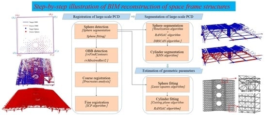
To create a BIM model of a structural component, geometrical parameters or features, such as section dimensions, lengths, corners, and lines, are essential [44]. Hence, the problem of accurate inverse modeling can be considered in how to accurately estimate dimensions. For steel structural components, Cabaleiro et al. [16] proposed a method to automatically generate a 3D model of frame connections by using the Hough transform to detect lines in 2.5D data. Based on the analysis of these detected lines, geometric and topological information about the frame connections can be obtained. All geometric results can be imported to commercial BIM software to create 3D models. Cabaleiro et al. [45] also generated as-built BIM models of deformed steel beams by hyperplane fitting and critical edge extraction based on the Hough transform. To automatically obtain a 3D BIM model of a steel frame, Laefer and Truong-Hong [17] determined the main sections of each steel component by using the robust principal component analysis (RPCA). Each section’s data was compared with standard sections in the database to determine the best matching dimensions. The as-built model was then generated from the standard model. Liu et al. [46] developed a method to model and analyze the structural performance of curved steel components based on PCD collected by a 3D handheld scanner, which requires close scanning distances. Yang et al. [18] proposed a semi-automated method to create the as-built BIM model for structural steel bridges. They manually segmented the target data to be reconstructed and used region growing to extract each component data. The center axis and section dimensions are then estimated for different types of steel components by using PCA and RANSAC. The model of the extracted component was created according to the estimated parameters, but the undetected components were created manually. Although the above methods are effective for specific targets, with the exception of the method proposed by Yang et al. [18], none of the above studies are applicable to full-scale structural components with complex relationships. Yang et al. [18] provide a good technical route for the 3D reconstruction of steel structures. The accuracy of their dimensional estimation method is reliable, but the preprocessing method is not suitable for space grid structures with a lot of background noise and a large number of members with complex connection relationships. Therefore, inspired by the above studies, this study will focus on the preprocessing of the space frame data and apply the RANSAC algorithm to dimensional estimation in order to efficiently and accurately obtain control parameters for the 3D reconstruction of space frame structural components.

3. Methodology

This study proposes a semi-automated and effective approach to generate the as-built BIM model for a full-scale space frame structure with terrestrial laser scanning data. The proposed approach involves the following three steps: (1) the registration of large-scale PCD; (2) the segmentation of large-scale PCD; and (3) the estimation of geometric parameters. Figure 2 shows the flowchart for generating the as-built BIM model.

3.1. Registration of Large-Scale PCD

A novel PCD registration method, known as Target Oriented Bounding Box–Iterative Closest Point (TO–ICP), is proposed specifically for space frame structures in this study, which includes sphere detection, OBB detection, coarse registration, and fine registration.

The sphere detection was processed on spherical joints (400–800 mm in diameter), being widely distributed in a space frame structure, including sphere segmentation and sphere fitting, as described in Section 3.2.1 and Section 3.3.1, respectively. Considering the fact that a large number of spherical joints can be scanned by a terrestrial laser scanner at each station, the correspondences between spherical joints are difficult to be directly identified. Although four-point congruent set (4PCS) technology [22,47] is effective in establishing correspondences between two subsets, obtaining the congruent set of tuples can also be challenging for 4PCS due to similar spatial arrangements of spherical joints. To address this issue, the OBB of space frame structures was adopted to globally locate detected spheres. The terrestrial laser scanner is generally leveled, and most modern scanners are capable of making a leveling compensation for slight tilting. Therefore, the PCD can be directly projected to a horizontal plane. Consequently, the OBB can be detected by the functions of cvFindContours and cvMinAreaRect2 [48], based on the binary images generated by two-dimensional (2D) PCD on the horizontal plane, as illustrated in Figure 3. The OBB matching is performed at the four corners represented by A, B, C, and D. Therefore, there are two candidate matchings between different OBBs obtained, respectively, from the target PCD and source PCD, as depicted in Figure 4. From the two candidate matchings, the one with a larger number of sphere correspondences (k) can be chosen. Considering m spheres {S_i} from source PCD and n spheres {T_i} from target PCD, k is given as

$$k={\displaystyle \sum }_{\mathrm{i}=1}^m{\displaystyle \sum }_{j=1}^n\eta \left(\sqrt{{(S_{\mathrm{ix}}-T_{\mathrm{jx}})}^2+{(S_{\mathrm{iy}}-T_{\mathrm{jy}})}^2}\right)$$

(1)

where S_ix and S_iy are, respectively, the x and y coordinates of S_i; T_jx and T_jy are, respectively, the x and y coordinates of T_i; and the function η($\odot$) is defined as

$$\eta \left(\odot \right)=\left\{\begin{array}{cc}0& \odot >D_{\lim }\\ 1& \odot <D_{\lim }\end{array}\right.$$

(2)

where D_lim represents the threshold distance. Coarse registration was performed on the sphere correspondences with η = 1 denoted as <S, T>. Based on <S, T>, Procrustes analysis technique [49] was adopted to estimate the rotation matrix R and translation matrix t, which are given as

$$W={\displaystyle \sum }_{\mathrm{i}=1}^k\left(S_{\mathrm{i}}-{\mu }_{\mathrm{S}}\right){\left(T_{\mathrm{i}}-{\mu }_{\mathrm{T}}\right)}^T$$

(3)

$$W=U\Sigma V^T$$

(4)

$$\mathit{R}=U{V}^T$$

(5)

$$\mathit{t}={\mu }_{\mathrm{T}}-R{\mu }_{\mathrm{S}}$$

(6)

where S_i and T_i are, respectively, the 3D coordinate vectors of the source and target spheres contained in <S, T>; μ_S and μ_T are, respectively, the mean vectors of S_i and T_i; U, ∑, and V are obtained from matrix W using the singular value decomposition. The coarse registration of large-scale PCD is shown in Figure 5a.

The coarse registration only uses the centers of detected spheres. Therefore, the registration quality of the coarse registration to be guaranteed is entirely dependent on the accuracy of the sphere estimation. Therefore, the PCD was finely adjusted by the ICP algorithm [21]. The fine registration of large-scale PCD is shown in Figure 5b. Moreover, Figure 5c shows the data registration result using the FPFH algorithm for comparison. The FPFH algorithm calculates high-dimensional point features and performs feature correspondence based on the RANSAC algorithm. It can be noticed that direct data registration based on point features fails as there are numerous background noises and repetitive structures.

3.2. Segmentation of Large-Scale PCD

3.2.1. Sphere

For large-scale PCD, the estimation of normal vectors and curvature is time-consuming and very sensitive to noises and outliers. To overcome this drawback, a novel parallelizable method is proposed for extracting the sphere targets from full-scale structures based on the voxelization algorithm and RANSAC algorithm.

First, large-scale PCD were subdivided into supervoxels of the size D_max × D_max × D_max, using the voxelization algorithm [50], as shown in Figure 6, where D_max represents the largest diameter of the spheres contained in a space frame structure, which can be easily obtained from the design information.

Second, the RANSAC algorithm was adopted to detect the sphere in each supervoxel. For each point set {p} contained in a supervoxel, random subsets with four points are selected and used to fit the sphere. The fitted spheres are then evaluated by a function C given as

$$C={\displaystyle \sum }_{\mathrm{i}}\rho (e_{\mathrm{i}}^2)$$

(7)

where e_i is the distance between the fitted sphere surface and the ith point, and ρ is a function defined as

$$\rho \left(e_{\mathrm{i}}^2\right)=\left\{\begin{array}{cc}1& e_{\mathrm{i}}^2\le t^2\\ 0& e_{\mathrm{i}}^2>t^2\end{array}\right.$$

(8)

where t is a threshold that can be preset according to accuracy requirements and is taken as 2 mm in this study. The key parameter for the RANSAC algorithm is the number of iterations I_n, which can be determined through the Monte Carlo type probabilistic approach given as

$$I_n=\frac{\mathit{lg}\left(1-w\right)}{\mathit{lg}(1-{\epsilon }^4)}$$

(9)

where w is a coefficient usually set as 0.99, and ε is the percentage of inliers calculated adaptively by

$$\epsilon =n_{\mathrm{p}}/n_{\mathrm{t}}.$$

(10)

where n_t is the number of points contained in {p_i}, and n_p is the minimum number of required points empirically set as 300 in this study. If the diameter estimated by the RANSAC algorithm ranges from 0.5D_max to D_max, the inliers will be selected into a set denoted as {p_s}.

Last, the points contained in {p_s} are clustered by using the Density-Based Spatial Clustering of Applications with Noise (DBSCAN) algorithm [51]. Figure 7 illustrates 42 spheres successfully segmented from the large-scale PCD shown in Figure 6. It is worth noting that the analysis of the PCD in these supervoxels is independent and can be carried out in a parallel manner. Even though the RANSAC requires several calculations in each supervoxel, the efficiency is still acceptable.

3.2.2. Cylinder

Cylindrical steel tubes are connected by two adjacent spherical joints, serving as the prior knowledge for extracting cylinder PCD. A fast and easy method is proposed in this study to extract the cylinder PCD of a space frame structure (FE-eCylinder), including the building relationship between spheres and the extracting cylinder PCD by k-Nearest Neighbors (kNN) with a radius threshold [52].

For each detected sphere represented by 0, as depicted in Figure 8, a kNN with a radius threshold (r_max) is used to establish the candidate relationships (i.e., 0–1, 0–2, 0–4, 0–5, 0–6, 0–7, 0–8, 0–9) between spheres, where r_max is set as the maximum length of steel tubes. Any unreasonable relationship 0–i (i.e., 0–2) should be removed provided that the following condition is satisfied:

$${\theta }_{\mathrm{ij}}\le {\theta }_{\mathrm{limit}}\&\&L_{\mathrm{i}}>L_{\mathrm{j}}$$

(11)

where i is j $\in$ {1,2,3,4,5,6,7,8,9}; θ_ij denotes the angel between vectors 0–i and 0–j; θ_limit is taken as 10° for actual space frame structures; L_i and L_j represent, respectively, the lengths of Lines 0i and 0j.

Based on the reasonable relationships between spheres (0–1, for example), a rough PCD extraction is first conducted on Point D by kNN with the radius threshold equal to half the length of Line 01 (Figure 9), where Point D denotes the midpoint of Line 01. Second, a fine PCD extraction is conducted based on Line AB. To overcome the negative effects of sphere PCD on the cylinder PCD extraction, Line AB should be shorter than Line 01. In this study, the lengths of 0A and B1 were empirically taken as 1.2 times the sphere radius, which does not affect the parameter estimation of the cylinder PCD. Other lengths that achieve the same effect are also feasible. Line AB was divided into n equal increments. For each equal increment, the kNN, with a radius threshold of 0.2 m being the maximum radius of the steel tube, was processed to extract the cylinder PCD. A factor η was calculated by

$$\eta =m/n$$

(12)

where m denotes the number of equal increments containing neighbors. If η is larger than 50%, the extracted cylinder PCD is considered to be reliable.

3.3. Estimation of Geometric Parameters

3.3.1. Sphere

As the sphere PCD obtained by the method described in Section 3.2.1 has no outliers and is reliable, the least squares algorithm can be adapted to fit the sphere. Figure 10 shows two examples of extracted sphere PCD (blue) and the spheres fitted by the least squares algorithm (cyan). A sphere in the cartesian coordinate system can be described by Equation (13) with the center coordinate (x_c, y_c, z_c) and radius r:

$${(x_{\mathrm{i}}-x_{\mathrm{c}})}^2+{(y_{\mathrm{i}}-y_{\mathrm{c}})}^2+{(z_{\mathrm{i}}-z_{\mathrm{c}})}^2=r^2$$

(13)

where x_i, y_i, z_i (i = 1, 2, …, n) are the coordinates of sphere PCD, and x_c, y_c, z_c, and r can be obtained by Equations (14) and (15):

$$\left[\begin{array}{c}-2x_{\mathrm{c}}\\ -2y_{\mathrm{c}}\\ -2z_{\mathrm{c}}\\ x_{\mathrm{c}}^2+y_{\mathrm{c}}^2+z_{\mathrm{c}}^2-r^2\end{array}\right]={(E^{T}E)}^{-1}{E}^{T}F$$

(14)

$$E=\left[\begin{array}{cccc}{x}_1& y_1& z_1& 1\\ x_2& y_2& z_2& 1\\ x_3& y_3& z_3& 1\\ x_4& y_4& z_4& 1\\ •& •& •& •\\ x_{\mathrm{n}}& y_{\mathrm{n}}& z_{\mathrm{n}}& 1\end{array}\right]F=\left[\begin{array}{c}-x_1^2-y_1^2-z_1^2\\ -x_2^2-y_2^2-z_2^2\\ -x_3^2-y_3^2-z_3^2\\ -x_4^2-y_4^2-z_4^2\\ •\\ -x_{\mathrm{n}}^2-y_{\mathrm{n}}^2-z_{\mathrm{n}}^2\end{array}\right]$$

(15)

3.3.2. Cylinder

Realizing that the cylinder centerline is approximate to Line 01 (Figure 11a), the cutting plane perpendicular to Line 01 was adopted to extract the cross-sectional PCD set, based on which a series of centers can be obtained using the RANSAC algorithm. The cylinder centerline can then be estimated based on these obtained centers using the RANSAC algorithm, as depicted in Figure 11b. The cylinder PCD projected along the cylinder centerline was adopted to estimate the cylinder radius using the RANSAC algorithm, as shown in Figure 11c. With these steps described above, the cylinder can be effectively fitted.

4. An Application in Full-Scale Space Frame Structures

4.1. Data Collection

To validate the proposed approach for generating the as-built BIM model for full-scale space frame structures with terrestrial laser scanning data, a real-world space frame structure located at Luzhou in Sichuan Province (China) was scanned using FARO S150 [53]. Multiple scans were made at 22 locations, as indicated in Figure 12a, where #1–#7 and #16–#22 were scanned with an angular resolution of 0.07°, and #8–#15 were with an angular resolution of 0.036°. These scanner locations were initially determined based on the results of scan planning [54] and then were supplemented by the scanner operators based on site conditions and their experience. To ensure successful registration, adjacent scanned PCD should be overlapped with at least three spherical joints, which was ensured by a scanner operator. Figure 12b shows an actual photo of data collection in the field. All scanned PCD were pre-processed by sub-sampling with the size of 10 mm using a personal computer of Intel Core i7-7700k CPU @ 4.20GHz made in China. All algorithms are implemented in Python.

Table 1. Summary of scanned PCD.

Location	Original/Sampling Points	Location	Original/Sampling Points
#1	13,988,195/5,368,352	#2	16,275,140/7,570,197
#3	15,392,697/7,544,656	#4	13,397,295/9,125,325
#5	13,707,609/9,275,676	#6	12,143,921/7,807,302
#7	21,742,499/9,807,240	#8	59,541,256/14,504,592
#9	58,729,766/15,087,340	#10	59,910,220/14,766,215
#11	48,133,412/14,796,388	#12	37,703,339/12,295,436
#13	56,738,434/14,511,595	#14	54,680,413/14,092,693
#15	36,803,597/13,461,163	#16	13,339,396/6,231,241
#17	13,152,792/5,565,005	#18	13,997,682/5,975,098
#19	18,719,062/11,503,259	#20	18,436,252/12,229,958

lists the details of scanned PCD, with each having the approximate dimensions of 125 m × 120 m × 10 m.

4.2. Results and Discussion

4.2.1. Registration of Large-Scale PCD

Typically registered scans are shown in Figure 13. To evaluate the TO–ICP method, the rotation error e_R, translation error e_T, and consumption time are introduced, where e_R and e_T are defined as

$${\mathit{e}}_{\mathrm{R}}=\mathit{arccos}(\frac{\mathrm{tr}\left({\mathit{R}}_{\mathrm{c}}\right)-1}{2})-\mathit{arccos}(\frac{\mathrm{tr}\left({\mathit{R}}_{\mathrm{t}}\right)-1}{2})$$

(16)

$${\mathit{e}}_{\mathrm{T}}=||{\mathit{t}}_{\mathrm{c}}-{\mathit{t}}_{\mathrm{t}}||$$

(17)

where R_c and t_c are, respectively, the rotation and translation matrices estimated by the TO–ICP method; R_t and t_t are, respectively, the ground truth rotation and translation matrices generated by the manual registration. As indicated in

Table 2. Typical details of large-scale PCD registration.

Target PCD	Source PCD	eR (°) *			eT (mm)	Computation Time (s) **
		ex	ey	ez		1	2	3	4
#1	#2	0	0	0	0.0001	6558	12	6	120
#8	#9	0	0	0	0.00004	3882	30	35	119
#12	#13	0	0	0	0.0002	3715	27	19	113
#17	#18	0	0	0	0.00008	5981	11	4	119

* e_x, e_y, and e_z are, respectively, the rotation errors in x, y, and z directions; ** 1 represents the sphere detection; 2 represents the OBB detection; 3 represents the coarse registration; 4 represents the fine registration.

, both e_R and e_T are approximately equal to zero, demonstrating the accuracy of the TO–ICP method. The consumption time ranges from 3874 s to 6696 s, with sphere detection accounting for the most. The registration results of the 22 scanned PCDs are shown in Figure 14, containing 235,391,564 points.

4.2.2. Segmentation of Large-Scale PCD

To evaluate the VR-eSphere and FE-eCylinder methods, a PCD with 5,208,163 points, as shown in Figure 6, was processed. Since accurate sphere detection can guarantee successful data registration, this study further illustrates the advantages of the proposed method in the coarse registration process by comparing VR-eSphere with a curvature-based method. The comparison of sphere PCD segmentation is illustrated in Figure 15, where the detected points are distinguished by red color. As seen, there are many errors in sphere PCD segmentation in the curvature-based method induced by outliers, while all points detected by the VR-eSphere method are correct, demonstrating that this method is robust to noises and outliers. However, the time consumed in the VR-eSphere method is relatively longer. Figure 16 shows the comparison of cylinder PCD segmentation, from which it can be concluded that the FE-eCylinder method is more accurate and effective than the curvature-based method. It is worth mentioning that the FE-eCylinder is limited to space frame structures.

In this study, since there are no incorrectly detected objects but only missed objects in the event of a detection failure, the segmentation results are evaluated by

$$Recall=TP/\left(TP+FN\right)$$

(18)

where TP is a true positive, representing the number of detected components, and FN is a false negative, representing the number of undetected components.

As shown in Figure 17 and

Table 3. Evaluation of the proposed segmentation method.

Item	Sphere	Cylinder	Total
Recall (%)	94.4%	94.1%	94.1%

, 802 out of 850 spheres were successfully extracted from the 22 sets of scanned PCDs and registered in a unified coordinate. It is worth noting that 48 spheres were not detected because these component data may be sparse due to being occluded by some background objects, such as protective nets and scaffolding. Based on the detected spheres, 3099 out of 3295 cylinders (Figure 18) were successfully extracted from the registered PCD, as shown in Figure 18. Therefore, the segmentation method proposed in this study has a high recall rate of about 94%.

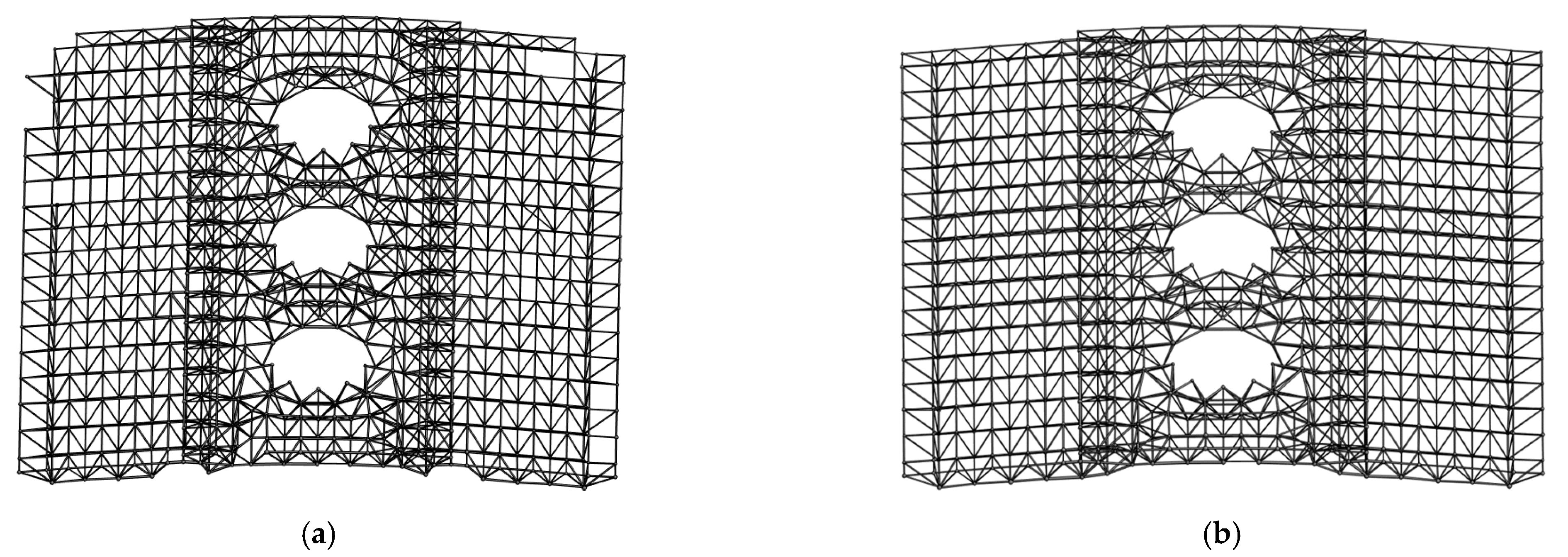
4.2.3. BIM Reconstruction

Based on the estimated geometric parameters sorted in a text file, a solid-based family was adopted to form the components through the use of the Revit application programming interface (API). All successfully detected components (about 94%) can be automatically generated as solid units based on their estimated dimensions, as shown in Figure 19a. However, components that fail detection (about 6%) require manual inverse modeling based on their PCDs, as shown in Figure 19b. As it takes about 6 h to achieve an automated BIM reconstruction of about 94% of the total components using the proposed approach, compared to a total of approximately 100 h using manual inverse modeling for all components, this demonstrates a significant improvement in the efficiency of the BIM model reconstruction of the space frame structure by using the proposed approach. Figure 19c shows the effect of overlaying the PCD without background noise on the as-built model. To evaluate the accuracy of the as-built model, the as-built model is discretized into a set of dense PCD [44] and considered as a reference. The distance between each point in the space frame PCD and its corresponding nearest neighbor in the as-built model PCD is calculated and shown in Figure 19d. From the frequency distribution corresponding to the absolute distances in Figure 19d, it can be seen that most of the points have an absolute distance of less than 0.01 m. The accuracy of this generated as-built model is acceptable for subsequent engineering management applications.

To further assess the as-built BIM model accuracy, this study evaluates the results of the parameter estimation of the detected components. As the estimation of the dimensions of both spherical joints and cylindrical steel tubes is based on the RANSAC algorithm, which has a close error accuracy, only the estimation accuracy of the spherical joints is discussed here. Diameter estimates for two different diameters of spherical joints in the space frame structure are used to compare with the design values.

Table 4. Allowable errors specified in the Chinese code GB 50205-2020 [55].

Items	Allowable Errors ${\mathit{\delta }}_{\mathit{s}}$
Ds <= 300 mm	±1.5 mm
300 mm < Ds <= 500 mm	±2.5 mm
500 mm < Ds <= 800 mm	±3.5 mm
Ds > 800 mm	±4.0 mm

lists the allowable errors ${\delta }_{\mathrm{s}}$ specified in the Chinese code GB 50205-2020 [55], where D_s represents the as-designed diameter of a sphere. When the discrepancy between an estimate and a design value is within the tolerance defined in the specification, it demonstrates that the cumulative error consisting of manufacturing and algorithm is acceptable. The comparison results are given in Figure 20. As seen, 90% and 78% of satisfactory results are reached, respectively, for 450 mm- and 600 mm-diameter spherical joints. The majority of the spherical joints meet the specification requirements, and those that exceed them have errors very close to the tolerances, which demonstrates that the as-built model is reliable for subsequent management operation and maintenance.

5. Conclusions

This study describes an effective semi-automated approach for generating the as-built building information modeling (BIM) model for a full-scale space frame structure with terrestrial laser scanning data by including the large-scale point cloud data (PCD) registration, large-scale PCD segmentation, and geometric parameter estimation. A case study conducted on a full-scale space frame structure was used to verify the validity of the proposed approach. The main conclusions of this study include the following:

(1)

The proposed TO–ICP enables the automatic registration of PCD of space frames with high accuracy;

(2)

The total computation time of the proposed VR-eSphere and FE-eCylinder is approximately half that of the curvature-based feature detection methods;

(3)

Although manual modeling is required for undetected components, the proposed BIM reconstruction approach significantly improves the efficiency of obtaining the as-built BIM model of full-scale space frame structures with cylindrical and spherical components. The effectiveness and reliability of the method are demonstrated by its application in the actual space frame structure.

However, this study still has some limitations. TO–ICP may not be suitable for the space frame structure with a circular shape as the OBB of different scanned data does not have significant differences. FE-eCylinder cannot be used for the detection and dimensional estimation of curved components because the key to fitting the curved component is the extraction of the central axis. Moreover, the PCD of undetected components needs to be modeled manually, which is still a time-consuming task. Therefore, in future work, research should be undertaken to improve the quality of collected PCD and to improve the accurate extraction of undetected components from PCD. The effective registration of space frames with circular shapes and the automatic inverse modeling of curved components will be further investigated.

References

1. El-Sheikh, A. Approximate dynamic analysis of space trusses. Eng. Struct. 2000, 22, 26–38. [Google Scholar] [CrossRef]
2. Toğan, V.; Daloğlu, A.T. Optimization of 3d trusses with adaptive approach in genetic algorithms. Eng. Struct. 2006, 28, 1019–1027. [Google Scholar] [CrossRef]
3. Silva, W.V.; Bezerra, L.M.; Freitas, C.S.; Bonilla, J.; Silva, R. Use of Natural Fiber and Recyclable Materials for Spacers in Typical Space Truss Connections. J. Struct. Eng. 2021, 147, 04021112. [Google Scholar] [CrossRef]
4. Zhao, P.; Liao, W.; Huang, Y.; Lu, X. Intelligent beam layout design for frame structure based on graph neural networks. J. Build. Eng. 2023, 63, 105499. [Google Scholar] [CrossRef]
5. Chen, Y.; Lu, C.; Yan, J.; Feng, J.; Sareh, P. Intelligent computational design of scalene-faceted flat-foldable tessellations. J. Comput. Des. Eng. 2022, 9, 1765–1774. [Google Scholar] [CrossRef]
6. Zhang, P.; Fan, W.; Chen, Y.; Feng, J.; Sareh, P. Structural symmetry recognition in planar structures using convolutional neural networks. Eng. Struct. 2020, 260, 114227. [Google Scholar] [CrossRef]
7. Chen, Y.; Yan, J.; Sareh, P.; Feng, J. Nodal flexibility and kinematic indeterminacy analyses of symmetric tensegrity structures using orbits of nodes. Int. J. Mech. Sci. 2019, 155, 41–49. [Google Scholar] [CrossRef]
8. Azhar, S. Building information modeling (BIM): Trends, benefits, risks, and challenges for the AEC industry. Leadersh. Manag. Eng. 2011, 11, 241–252. [Google Scholar] [CrossRef]
9. Woo, J.; Wilsmann, J.; Kang, D. Use of as-built building information modeling. In Proceedings of the Construction Research Congress 2010: Innovation for Reshaping Construction Practice, Banff, AB, Canada, 8–10 May 2010; pp. 538–548. [Google Scholar]
10. Tang, P.; Huber, D.; Akinci, B.; Lipman, R.; Lytle, A. Automatic reconstruction of as-built building information models from laser-scanned point clouds: A review of related techniques. Autom. Constr. 2010, 19, 829–843. [Google Scholar] [CrossRef]
11. Ma, Z.; Liu, S. A review of 3D reconstruction techniques in civil engineering and their applications. Adv. Eng. Inform. 2018, 37, 163–174. [Google Scholar] [CrossRef]
12. Wang, Q.; Kim, M.-K. Applications of 3D point cloud data in the construction industry: A fifteen-year review from 2004 to 2018. Adv. Eng. Inform. 2019, 39, 306–319. [Google Scholar] [CrossRef]
13. Zhang, Z.; Dai, Y.; Sun, J. Deep learning based point cloud registration: An overview. Virtual Real. Intell. Hardw. 2020, 2, 222–246. [Google Scholar] [CrossRef]
14. Cheng, L.; Chen, S.; Liu, X.; Xu, H.; Wu, Y.; Li, M.; Chen, Y. Registration of laser scanning point clouds: A review. Sensors 2018, 18, 1641. [Google Scholar] [CrossRef] [PubMed]
15. Xiong, X.; Adan, A.; Akinci, B.; Huber, D. Automatic creation of semantically rich 3D building models from laser scanner data. Autom. Constr. 2013, 31, 325–337. [Google Scholar] [CrossRef]
16. Cabaleiro, M.; Riveiro, B.; Arias, P.; Caamaño, J.C.; Vilán, J.A. Automatic 3D modelling of metal frame connections from LiDAR data for structural engineering purposes. ISPRS J. Photogramm. Remote Sens. 2014, 96, 47–56. [Google Scholar] [CrossRef]
17. Laefer, D.F.; Truong-Hong, L. Toward automatic generation of 3D steel structures for building information modelling. Autom. Constr. 2017, 74, 66–77. [Google Scholar] [CrossRef]
18. Yang, L.; Cheng, J.C.; Wang, Q. Semi-automated generation of parametric BIM for steel structures based on terrestrial laser scanning data. Autom. Constr. 2020, 112, 103037. [Google Scholar] [CrossRef]
19. Besl, P.J.; McKay, N.D. A method for registration of 3-D shapes. IEEE Trans. Pattern Anal. Mach. Intell. 1992, 14, 239–256. [Google Scholar] [CrossRef]
20. Yang, J.; Li, H.; Campbell, D.; Jia, Y. Go-ICP: A globally optimal solution to 3D ICP point-set registration. IEEE Trans. Pattern Anal. Mach. Intell. 2015, 38, 241–2254. [Google Scholar] [CrossRef]
21. Donoso, F.A.; Austin, K.J.; McAree, P.R. How do ICP variants perform when used for scan matching terrain point clouds? Robot. Auton. Syst. 2017, 87, 147–161. [Google Scholar] [CrossRef]
22. Mellado, N.; Aiger, D.; Mitra, N.J. Super 4pcs fast global point cloud registration via smart indexing. Comput. Graph. Forum 2014, 33, 205–215. [Google Scholar] [CrossRef]
23. Bosché, F. Plane-based registration of construction laser scans with 3D/4D building models. Adv. Eng. Inform. 2021, 26, 90–102. [Google Scholar] [CrossRef]
24. Rusu, R.B.; Blodow, N.; Beetz, M. Fast point feature histograms (FPFH) for 3D registration. In Proceedings of the IEEE International Conference on Robotics and Automation, Kobe, Japan, 12–17 May 2009; pp. 3212–3217. [Google Scholar]
25. Pan, X.; Lyu, S. Detecting image region duplication using SIFT features. In Proceedings of the IEEE International Conference on Acoustics: Speech and Signal Processing, Dallas, TX, USA, 14–19 March 2010; pp. 1706–1709. [Google Scholar]
26. Smith, S.M.; Brady, J.M. SUSAN—A new approach to low level image processing. Int. J. Comput. Vis. 1997, 23, 45–78. [Google Scholar] [CrossRef]
27. Pang, Y.; Li, W.; Yuan, Y.; Pan, J. Fully affine invariant SURF for image matching. Neurocomputing 2012, 85, 6–10. [Google Scholar] [CrossRef]
28. Aoki, Y.; Goforth, H.; Srivatsan, R.A.; Lucey, S. Pointnetlk: Robust & efficient point cloud registration using pointnet. In Proceedings of the IEEE/CVF Conference on Computer Vision and Pattern Recognition, Long Beach, CA, USA, 15–20 June 2019; pp. 7163–7172. [Google Scholar]
29. Lu, W.; Wan, G.; Zhou, Y.; Fu, X.; Yuan, P.; Song, S. Deepvcp: An end-to-end deep neural network for point cloud registration. In Proceedings of the IEEE/CVF International Conference on Computer Vision, Seoul, Republic of Korea, 27 October–2 November 2019; pp. 12–21. [Google Scholar]
30. Trimble, Trimble RealWorks. Available online: https://geospatial.trimble.com/products-and-solutions/trimble-realworks (accessed on 25 March 2023).
31. Geomagic, Geomagic Wrap. Available online: https://www.3dsystems.com/software/geomagic-wrap (accessed on 25 March 2023).
32. ClearEdge3D. EdgeWise. Available online: https://www.clearedge3d.com/products/edgewise (accessed on 25 March 2023).
33. Jung, J.; Hong, S.; Jeong, S.; Kim, S.; Cho, H.; Hong, S.; Heo, J. Productive modeling for development of as-built BIM of existing indoor structures. Autom. Constr. 2014, 42, 68–77. [Google Scholar] [CrossRef]
34. Patil, A.K.; Holi, P.; Lee, S.K.; Chai, Y.H. An adaptive approach for the reconstruction and modeling of as-built 3D pipelines from point clouds. Autom. Constr. 2017, 75, 65–78. [Google Scholar] [CrossRef]
35. Guo, J.J.; Wang, Q.; Park, J.H. Geometric quality inspection of prefabricated MEP modules with 3D laser scanning. Autom. Constr. 2020, 111, 103053. [Google Scholar] [CrossRef]
36. Adams, R.; Bischof, L. Seeded region growing. IEEE Trans. Pattern Anal. Mach. Intell. 1994, 16, 641–647. [Google Scholar] [CrossRef]
37. Mukhopadhyay, P.; Chaudhuri, B.B. A survey of Hough Transform. Pattern Recognit. 2015, 48, 993–1010. [Google Scholar] [CrossRef]
38. Pu, S.; Vosselman, G. Automatic extraction of building features from terrestrial laser scanning. Int. Arch. Photogramm. Remote Sens. Spat. Inf. Sci. 2006, 36, 25–27. [Google Scholar]
39. Schnabel, R.; Wahl, R.; Klein, R. Efficient RANSAC for point-cloud shape detection. Comput. Graph. Forum 2007, 26, 214–226. [Google Scholar] [CrossRef]
40. Abuzaina, A.; Nixon, M.S.; Carter, J.N. Sphere detection in kinect point clouds via the 3d hough transform. In Proceedings of the International Conference on Computer Analysis of Images and Patterns, York, UK, 27–29 August 2013; pp. 290–297. [Google Scholar]
41. Kawashima, K.; Kanai, S.; Date, H. As-built modeling of piping system from terrestrial laser-scanned point clouds using normal-based region growing. J. Comput. Des. Eng. 2014, 1, 13–26. [Google Scholar] [CrossRef]
42. Son, H.; Kim, C.; Kim, C. Fully automated as-built 3D pipeline extraction method from laser-scanned data based on curvature computation. J. Comput. Civ. Eng. 2015, 29, 765–772. [Google Scholar] [CrossRef]
43. Nguyen, C.H.P.; Choi, Y. Comparison of point cloud data and 3D CAD data for on-site dimensional inspection of industrial plant piping systems. Autom. Constr. 2018, 91, 44–52. [Google Scholar] [CrossRef]
44. Li, D.; Liu, J.; Feng, L.; Zhou, Y.; Qi, H.; Chen, Y.F. Automatic modeling of prefabricated components with laser-scanned data for virtual trial assembly. Comput.-Aided Civ. Infrastruct. Eng. 2021, 36, 453–471. [Google Scholar] [CrossRef]
45. Cabaleiro, M.; Riveiro, B.; Arias, P.; Caamaño, J. Algorithm for beam deformation modeling from lidar data. Measurement 2015, 76, 20–31. [Google Scholar] [CrossRef]
46. Liu, J.; Zhang, Q.; Wu, J.; Zhao, Y. Dimensional accuracy and structural performance assessment of spatial structure components using 3D laser scanning. Autom. Constr. 2018, 96, 324–336. [Google Scholar] [CrossRef]
47. Aiger, D.; Mitra, N.J.; Cohen-Or, D. 4-points congruent sets for robust pairwise surface registration. In Proceedings of the SIGGRAPH’08: Special Interest Group on Computer Graphics and Interactive Techniques Conference, Los Angeles, CA, USA, 11–15 August 2008. [Google Scholar]
48. Bradski, G.; Kaehler, A. Learning OpenCV: Computer Vision with the OpenCV Library; O’Reilly Media, Inc.: Sebastopol, CA, USA, 2008; Available online: https://opencv.org/ (accessed on 25 March 2023).
49. Case, F.; Beinat, A.; Crosilla, F.; Alba, I.M. Virtual trial assembly of a complex steel structure by Generalized Procrustes Analysis techniques. Autom. Constr. 2014, 37, 155–165. [Google Scholar] [CrossRef]
50. Karabassi, E.A.; Papaioannou, G.; Theoharis, T. A fast depth-buffer-based voxelization algorithm. J. Graph. Tools 1999, 4, 5–10. [Google Scholar] [CrossRef]
51. Louhichi, S.; Gzara, M.; Abdallah, H.B. A density based algorithm for discovering clusters with varied density. In Proceedings of the World Congress on Computer Applications and Information Systems, Hammamet, Tunisia, 17–19 January 2014; pp. 1–6. [Google Scholar]
52. Zhang, S.; Li, X.; Zong, M.; Zhu, X.; Wang, R. Efficient kNN Classification with Different Numbers of Nearest Neighbors. IEEE Trans. Neural. Netw. Learn. Syst. 2018, 29, 1774–1785. [Google Scholar] [CrossRef]
53. Faro. Faro Focus Laser Scanner User Manual. 2019. Available online: https://www.faro.com/en/Products/Hardware/Focus-Laser-Scanners (accessed on 25 March 2023).
54. Li, D.; Liu, J.; Zeng, Y.; Cheng, G.; Dong, B.; Chen, Y.F. 3D model-based scan planning for space frame structures considering site conditions. Autom. Constr. 2022, 140, 104363. [Google Scholar] [CrossRef]
55. GB 50205-2020; Standard for Acceptance of Construction Quality of Steel Structures. Ministry of Housing and Urban-Rural Development of PRC: Beijing, China, 2020. Available online: https://www.chinesestandard.net/China/Chinese.aspx/GB50205-2020 (accessed on 25 March 2023).
Figure 1. Typical space frame structure.
Remotesensing 15 02806 g001
Figure 2. The flowchart for generating the as-built BIM model.
Remotesensing 15 02806 g002
Figure 3. OBB detection: (a) source OBB; (b) target OBB.
Remotesensing 15 02806 g003
Figure 4. Two candidate matchings between different OBBs: (a) Case 1; (b) Case 2.
Remotesensing 15 02806 g004
Figure 5. Registration of source (blue) and target (red) PCD: (a) coarse registration by the TO–ICP method; (b) fine registration by the TO–ICP method; (c) coarse registration by the FPFH algorithm.
Remotesensing 15 02806 g005
Figure 6. Subdivision of large-scale PCD.
Remotesensing 15 02806 g006
Figure 7. Sphere segmentation from large-scale PCD by VR-eSphere (different spheres are numbered and distinguished by colors).
Remotesensing 15 02806 g007
Figure 8. Building relationships between spheres.
Remotesensing 15 02806 g008
Figure 9. Cylinder segmentation from large-scale PCD.
Remotesensing 15 02806 g009
Figure 10. Sphere fitting: (a) sphere 1; (b) sphere 2.
Remotesensing 15 02806 g010
Figure 11. Cylinder fitting: (a) cutting plane; (b) estimation of cylinder centerline; (c) estimation of cylinder radius.
Remotesensing 15 02806 g011
Figure 12. Basic information about data collection: (a) locations of multiple scans; (b) an actual photo of the construction site.
Remotesensing 15 02806 g012
Figure 13. Typical registered scans by TO–ICP (different scans are distinguished by colors): (a) #1 and #2; (b) #8 and #9; (c) #12 and#13; (d) #16 and #17.
Remotesensing 15 02806 g013
Figure 14. Registered results of 22 scanned PCDs.
Remotesensing 15 02806 g014
Figure 15. Comparison of the segmentation of sphere PCD, where the detected points are in red and the original points are in blue: (a) segmentation by VR-eSphere (computation time = 3683 s); (b) segmentation by the curvature-based method (computation time = 3360 s).
Remotesensing 15 02806 g015
Figure 16. Comparison of the segmentation of cylinder PCD, where the detected points are in red and the original points are in blue: (a) segmentation by FE-eCylinder (computation time = 11.7 s); (b) segmentation by the curvature-based method (computation time = 3232 s).
Remotesensing 15 02806 g016
Figure 17. Segmentation of sphere PCD.
Remotesensing 15 02806 g017
Figure 18. Segmentation of cylinder PCD.
Remotesensing 15 02806 g018
Figure 19. BIM reconstruction result: (a) the automatically generated as-built model; (b) the as-built model after manual completion; (c) the PCD of space frame structure superimposed on the as-built BIM model; (d) accuracy evaluation of the generated as-built model.
Remotesensing 15 02806 g019aRemotesensing 15 02806 g019b
Figure 20. Histogram of evaluation results: (a) Ds = 450 mm; (b) Ds = 600 mm.
Remotesensing 15 02806 g020