1. Introduction
Video synthetic aperture radar (SAR) combines SAR with high frame rate video display technology, which allows for continuous observation of targets at night and in harsh conditions such as rain, fog, sand, and dust [
1,
2]. As an inheritance and expansion of traditional SAR, video SAR can display information on ground motion targets in all directions [
3,
4]. Sandia National Laboratories (SNL) and Defense Advanced Research Projects Agency (DARPA) first proposed the concept of video SAR [
5], and then video SAR has been listed as a key research project by many countries and institutes. Currently, many institutions have published their video SAR systems and results, such as SNL [
6,
7], DARPA [
8], General Atomics Aeronautical Systems Incorporated (GA-ASI) [
9], Fraunhofer Institute for High-Frequency Physics and Radar Techniques (FHR) [
10], Jet Propulsion Laboratory (JPL) [
11], and ICEYE [
12,
13], which proves the importance and broad application value of video SAR.
SAR image formation can be treated as a class of ill-posed linear inverse problems [
14,
15], so the imaging algorithm is the core part of video SAR systems. The persistent imaging characteristics of video SAR require it to work in spotlight mode [
16]; therefore, the traditional strip SAR imaging algorithms, such as range Doppler algorithm (RDA) [
17], chirp scaling algorithm (CSA) [
18], and frequency scaling algorithm (FSA) [
19], are no longer applicable to video SAR. The current mainstream imaging algorithms for spotlight mode mainly include the back-projection algorithm (BPA) [
20,
21] and the polar format algorithm (PFA) [
22,
23,
24]. BPA requires point-by-point processing of echo signals, which makes its computational load too high to be applied in video SAR. The modified version, such as the fast back-projection algorithm (FBP) [
25] and the fast factorized back-projection algorithm (FFBP) [
26], has improved the efficiency of BPA, but this comes at the cost of losing imaging accuracy and is still less efficient than frequency-domain algorithms. PFA is the preferred imaging algorithm for video SAR due to its relatively high computational efficiency and ease of incorporating motion compensation algorithms [
27].
However, traditional PFA also has some problems. Firstly, the two-dimensional (2D) wavenumber domain interpolation is inefficient, which affects the efficiency of PFA. Secondly, due to the use of the planar wavefront approximation, the wavefront curvature error of PFA makes its effective scene size and image fidelity limited under the conditions of short slant range or large scene size [
28,
29,
30]. Thirdly, the video SAR frames should be oriented in a fixed direction on the ground output coordinate system (GOCS); otherwise, the image will rotate with the azimuth angle of video SAR [
31]. In [
32], by changing the sampling rate and sampling time of the radar system in real-time, the wavenumber domain signal with azimuth-uniform distribution can be obtained directly, while the azimuth chirp-z transform (
CZT) is used to avoid the wavenumber domain interpolation and has higher efficiency. In [
33], a parameter adjusting autoregistration PFA (PAAR-PFA) for linear spotlight mode video SAR is proposed; PAAR-PFA calculates the relevant parameters based on a parameter adjustment strategy to avoid range interpolation and geometric correction, but as in [
32], the system architecture has higher hardware cost, and the scene size limitation problem is still not solved. In [
34], a unified coordinate system algorithm (UCSA) is proposed for terahertz (THz) video SAR imaging; UCSA exploits the small-angle assumption property of THz video SAR, then a 2D
CZT is used to achieve wavenumber domain resampling and ignores the effect of residual quadratic phase error, showing the great advantages of THz technology [
35,
36] in video SAR. However, the UCSA cannot be applied well to low-band video SAR, which limits its application. In [
37], an efficient video SAR imaging algorithm based on type-3 non-uniform fast Fourier transform (NuFFT-3) is proposed by R. Hu; the method combines Fourier imaging and image correction to directly obtain distortion-free images. Then R. Hu extends the method to solve the defocusing problem, called refocusing and zoom-in PFA (RZPFA) [
28]. In [
38], the orthorectified polar format algorithm (OPFA) incorporates RZPFA with the digital elevation model (DEM); OPFA can obtain the orthorectified image efficiently without postprocessing, even with the residual distortion and defocus caused by rugged terrain.
To address the scene size limitation of PFA, some methods, such as spatially variant post filtering (SVPF) [
39,
40], are proposed to solve the defocus of imaging results. In [
41], an extended polar format algorithm (EPFA) is proposed to solve the wavenumber domain resampling and wavefront curvature error of squint SAR, but EPFA does not consider the geometric correction, which leads to the constant and primary terms of wavefront curvature error still exist and thus causes geometric distortion of the image. In [
42], a quadtree beam segmentation-based PFA is proposed to solve the image defocus problem of wide-angle staring SAR (WAS-SAR), but the computational load of this method increases significantly with the number of sub-beams. In [
43], an extended PFA is proposed to reduce the number of segmentations by combining sub-block imaging with spatially variant post-filtering. However, the extensive operation of image interpolation and alignment makes its computational complexity too high and, therefore, not suitable for application in video SAR.
In this paper, a generalized persistent polar format algorithm (GPPFA) is proposed to address the above problem. First, the imaging model of airborne video SAR is established, and the principles of high resolution and high frame rate of video SAR are analyzed. Then, the critical conditions of azimuth uniform and non-uniform resampling are analyzed, and the most suitable methods are used to achieve wavenumber domain resampling for THz video SAR and X-band video SAR, respectively. In addition, for the scene size limitation problem, the geometric distortion mapping (GDM) of video SAR PFA is established, and a residual phase error compensation method is proposed, which selects different processing procedures for different scene sizes to achieve higher operational efficiency. The main contributions of this paper are:
- (1)
The principle of wavenumber domain resampling in video SAR PFA is analyzed, and a resampling criterion applicable to different wavebands of video SAR is proposed;
- (2)
The effect of wavefront curvature error in video SAR PFA is analyzed, and an efficient compensation method applicable to different scene sizes is proposed;
- (3)
The proposed method is capable of video SAR fast imaging with high image fidelity in different wavebands, as well as arbitrary slant range and scene size.
The construction of the paper is organized as follows:
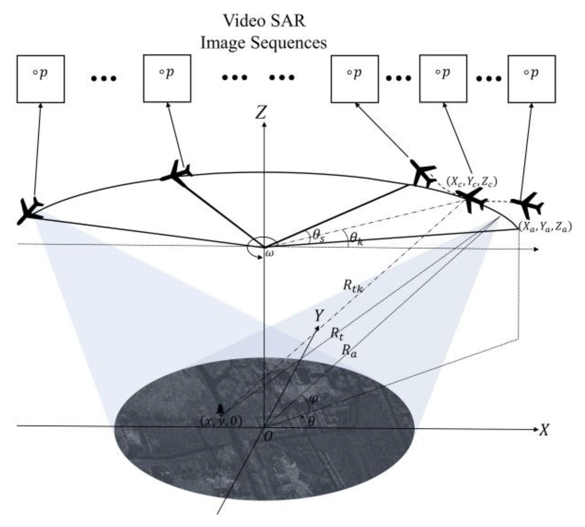
Section 2 establishes the airborne video SAR imaging model, analyzes the high-resolution and high-frame-rate imaging characteristics of video SAR, and briefly introduces the PFA in video SAR.
Section 3 analyzes the wavefront curvature error of PFA and discusses the proposed GPPFA in detail.
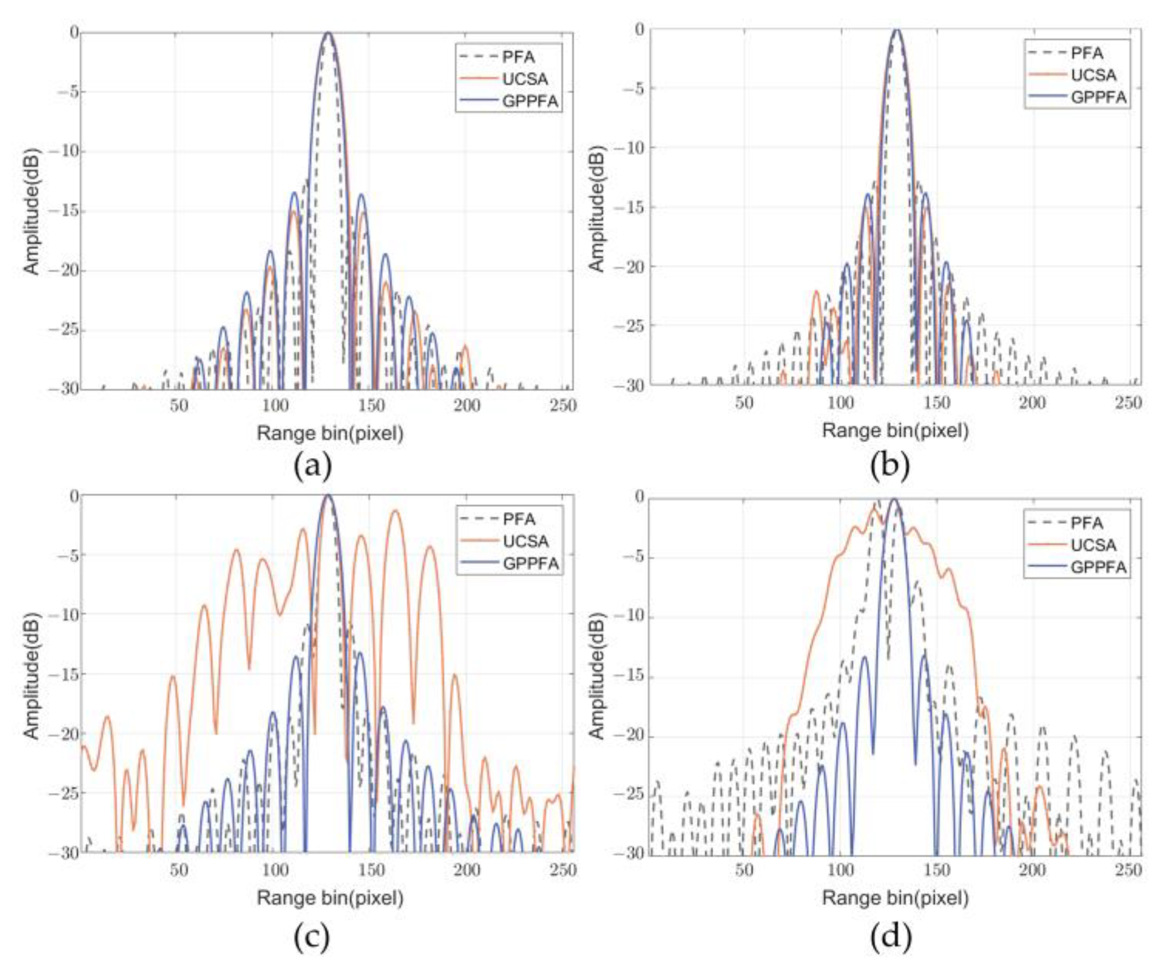
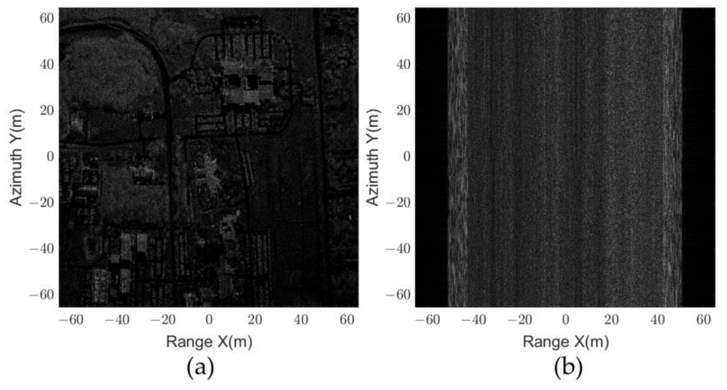
Section 4 validates the proposed method by point target and extended target experiments and compares it with other methods to verify the generality, effectiveness, and efficiency of the proposed method. Finally,
Section 5 summarizes the findings of the study.
3. Methods
There are still some problems when using PFA to process video SAR data. First, the 2D interpolation in the polar format transformation affects the computational efficiency of PFA. In addition, the wavefront curvature error leads to the limitation of the scene size of PFA. Considering the target localization tasks of video SAR, this wavefront curvature error must be corrected. To address the above issues, a generalized persistent polar format algorithm (GPPFA) is proposed to achieve a more efficient video SAR imaging that can be applied to different scenes.
3.1. Polar Format Transformation of GPPFA
The discrete form of range and azimuth wavenumber before PFA resampling can be expressed as:
where
is the range sample index such as
,
is the number of range sampling, n is the azimuth sample index such as
,
is the number of pulses.
There is a coupling between m and n in
and
, therefore, a polar-to-rectangular transformation should be carried out to remove the coupling [
48]. The range and azimuth wavenumber after resampling can be rewritten as:
To improve the efficiency, a 2D resampling is usually decomposed into range and azimuth resampling. The range wavenumber is always uniformly distributed, which is consistent with the sampling properties of
CZT [
49,
50]. For the azimuth resampling, it is not always uniformly distributed because the azimuth wavenumber is related to the azimuth angle. Therefore, more efficient
CZT can be used for range resampling, while for azimuth resampling, it can only be used within certain constraints.
CZT can actively set the start frequency and frequency interval, and it can calculate the Fourier transform of the signal on any arc on the unit circle. The z-transform of a sequence
is defined as:
where
and
are parameters of
CZT:
where
represents the start digital frequency,
is the digital frequency interval between adjacent two points.
The purpose of range resampling is to remove the coupling between range wavenumber
and pulse number
. Select the reference value as the range wavenumber at the azimuth index center
. Then, let
, the index before and after range resampling can be calculated as:
According to (21), the digital frequency after the range
CZT can be calculated as:
Therefore, the initial digital frequency
and the frequency interval
can be expressed as:
Then, the parameters of range
CZT are:
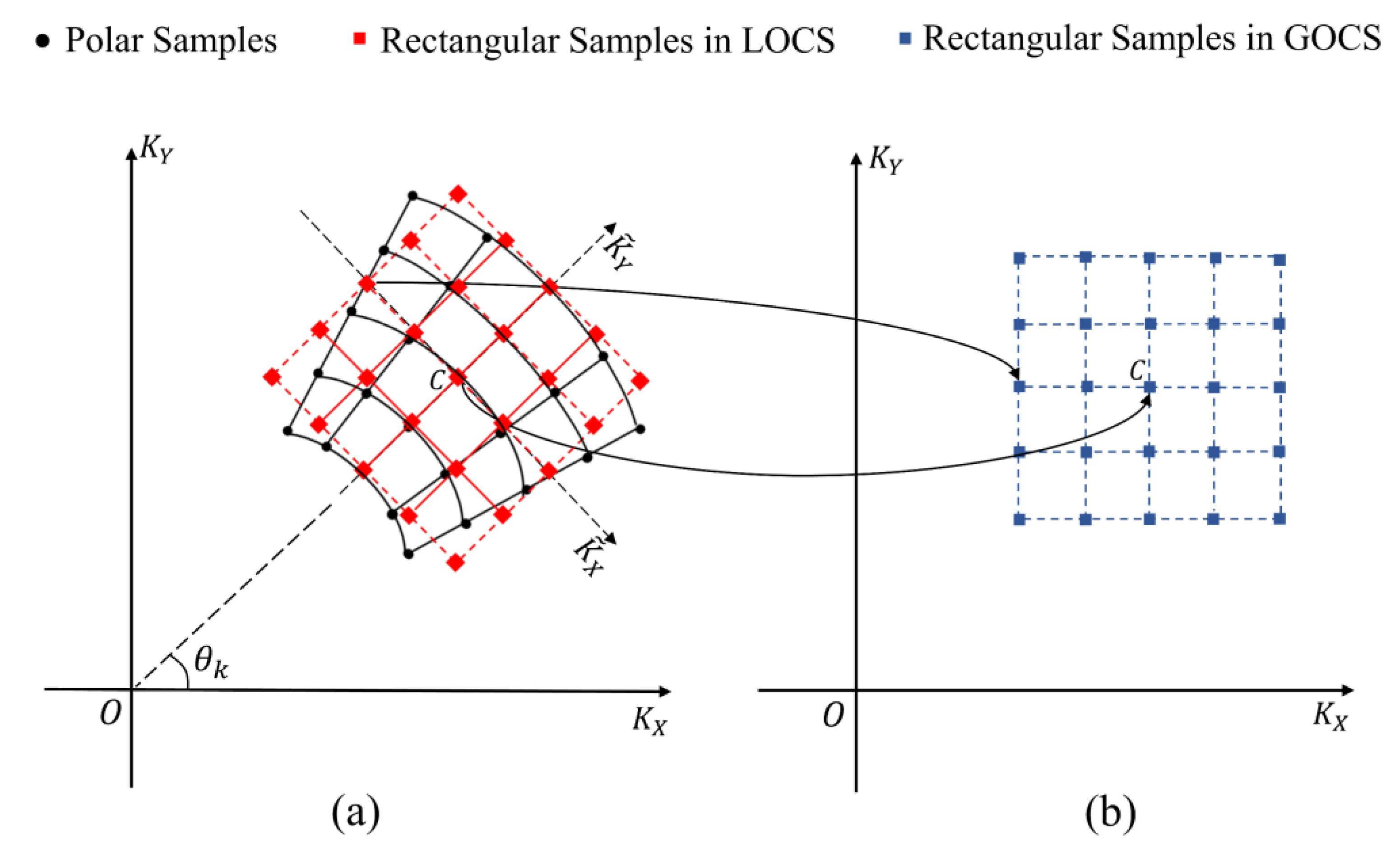
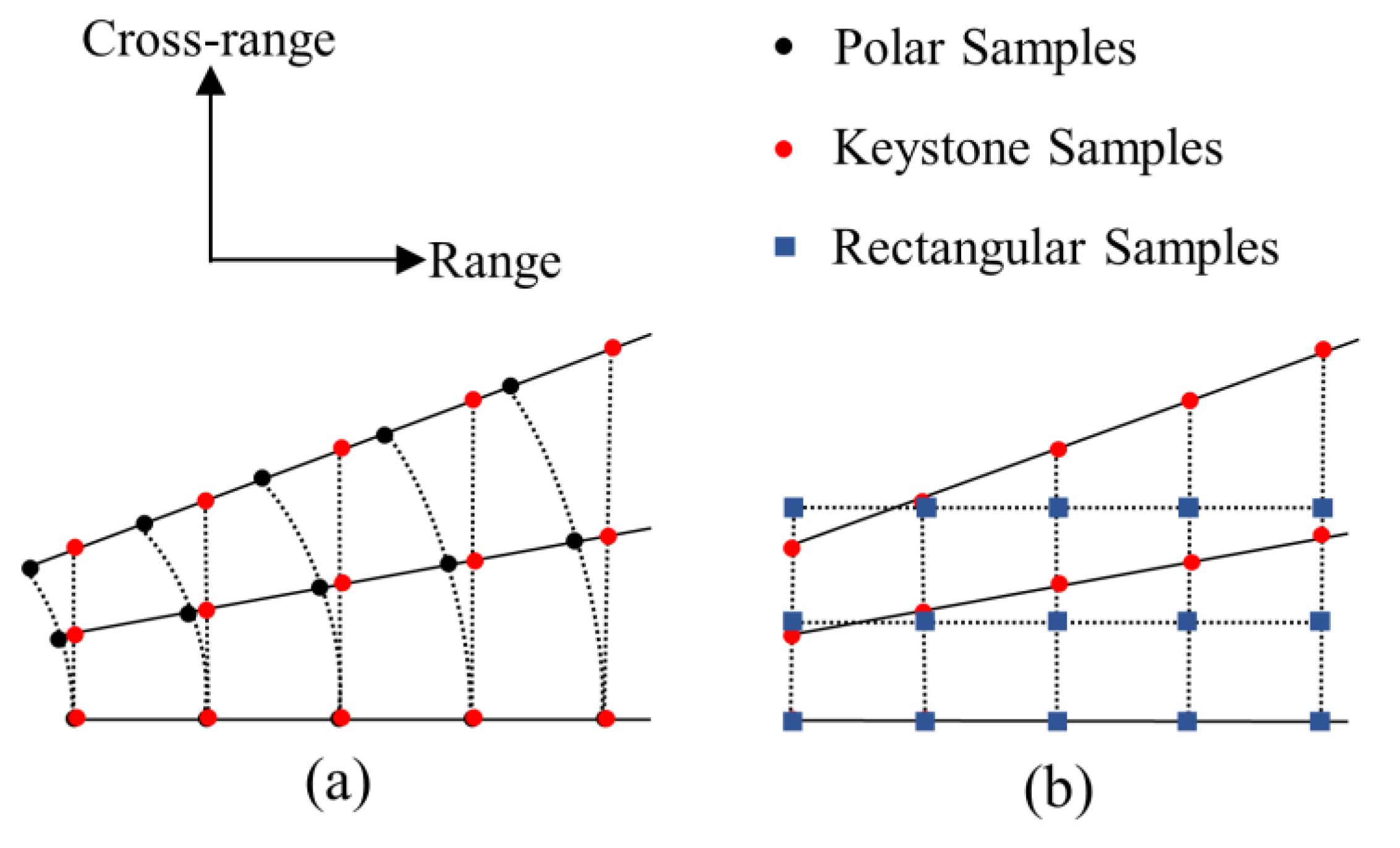
As shown in
Figure 3a, after the range
CZT, the wavenumber domain signal distribution is converted from a polar format to a keystone format, where the azimuth wavenumber
changes to the following form:
As shown in
Figure 3b, the purpose of azimuth resampling is to remove the coupling between azimuth wavenumber
and range index m. Select the reference value as the azimuth wavenumber at the range index center
. Then, let
:
Make the following approximation for (26):
The index before and after azimuth resampling can be calculated as:
According to (28), the digital frequency after the azimuth
CZT can be calculated as:
Therefore, the initial digital frequency
and the frequency interval
can be expressed as:
Then, the parameters of azimuth
CZT are:
The process of azimuth
CZT can be expressed as:
where
represents the azimuth
CZT,
is the range FFT.
The CZT-based azimuth resampling is based on a small-angle approximation of (27), which means that the azimuth wavenumbers are uniformly distributed; otherwise, it will lead to errors. Therefore, for the process of azimuth resampling, it is necessary to choose different processing methods according to different scenarios. For X-band video SAR (), the synthetic accumulation angle , while for THz video SAR () . Therefore, for THz video SAR, the azimuth CZT is sufficiently accurate, while X-band video SAR is not. To obtain an explicit criterion, it is necessary to derive the threshold for azimuth resampling.
Assume that the azimuth wavenumber is uniformly distributed in a two-dimensional wavenumber domain, then the azimuth phase error
can be written as:
where
can be approximated as
by Taylor series expansion, and the Taylor expansion of
can be expressed as:
A practical guideline is that the cubic error between two edges can be ignored if it does not exceed
π/4 [
51]. Therefore, the phase error
needs to satisfy:
The synthetic aperture angle
, then
can be expressed in the form of the carrier frequency:
Equation (36) reveals the information that the azimuth uniform resampling can be considered sufficiently accurate when is kept within the threshold.
Figure 4 shows the relationship between the frequency and scene size when the azimuth uniform resampling is satisfied. When
,
, and
, the frequency should satisfy
. Therefore, under this condition, X-band video SAR needs to use non-uniform azimuth resampling, such as interpolation, while THz video SAR can use a more efficient azimuth
CZT to complete the process of azimuth resampling. After the azimuth resampling is completed, a range IFFT is used to obtain the preliminary PFA image.
3.2. Wavefront Curvature Error Analysis and Compensation
The phase of the target can be expressed as:
Constant and linear phase errors lead to target offset, quadratic phase errors lead to image defocus, while higher-order phase errors have little impact on the image quality [
47]. Therefore, only constant terms, linear terms, and quadratic phase errors need to be considered, which decomposes wavefront curvature error compensation into geometric distortion correction and image defocus compensation.
From (37), it can be seen that the only term related to t in phase
is the differential distance
. Implementing the second order of Taylor series expansion to
and the approximate difference distance
at the aperture center moment
:
The constant terms are:
where
is the distortion position of the target
.
Associate the following relationships:
Then the following relationship can be obtained:
According to (42), the relationship between distortion position
and
is obtained, which is called GOCS geometric distortion mapping (GDM):
According to (16) and (43), the LOCS-GDM is obtained as:
Let
denotes the offset distance, and then the offset distance of the kth frame image is:
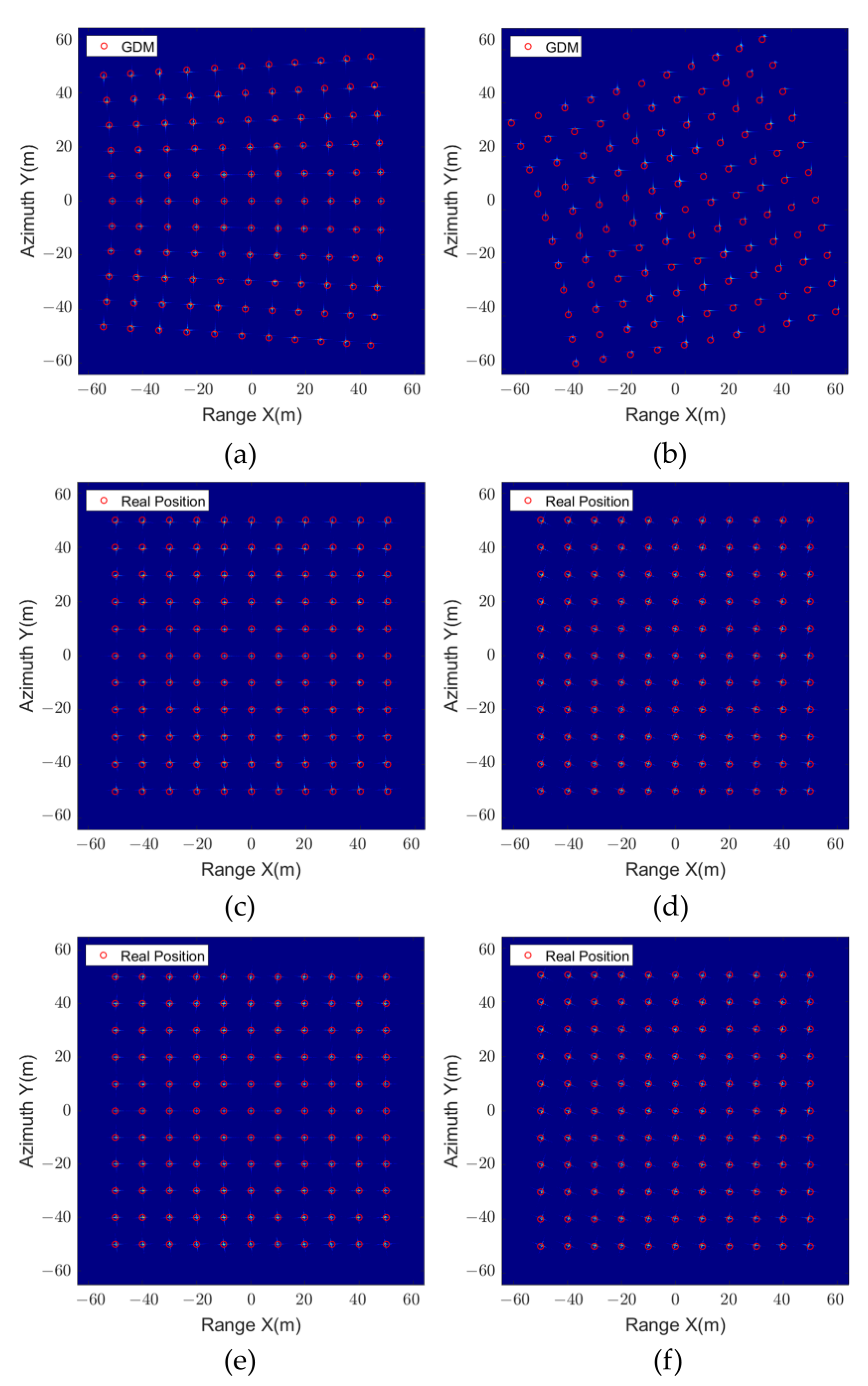
The effect of geometric distortion can be ignored only if it is within the distortion negligible region (DiR), which is defined as:
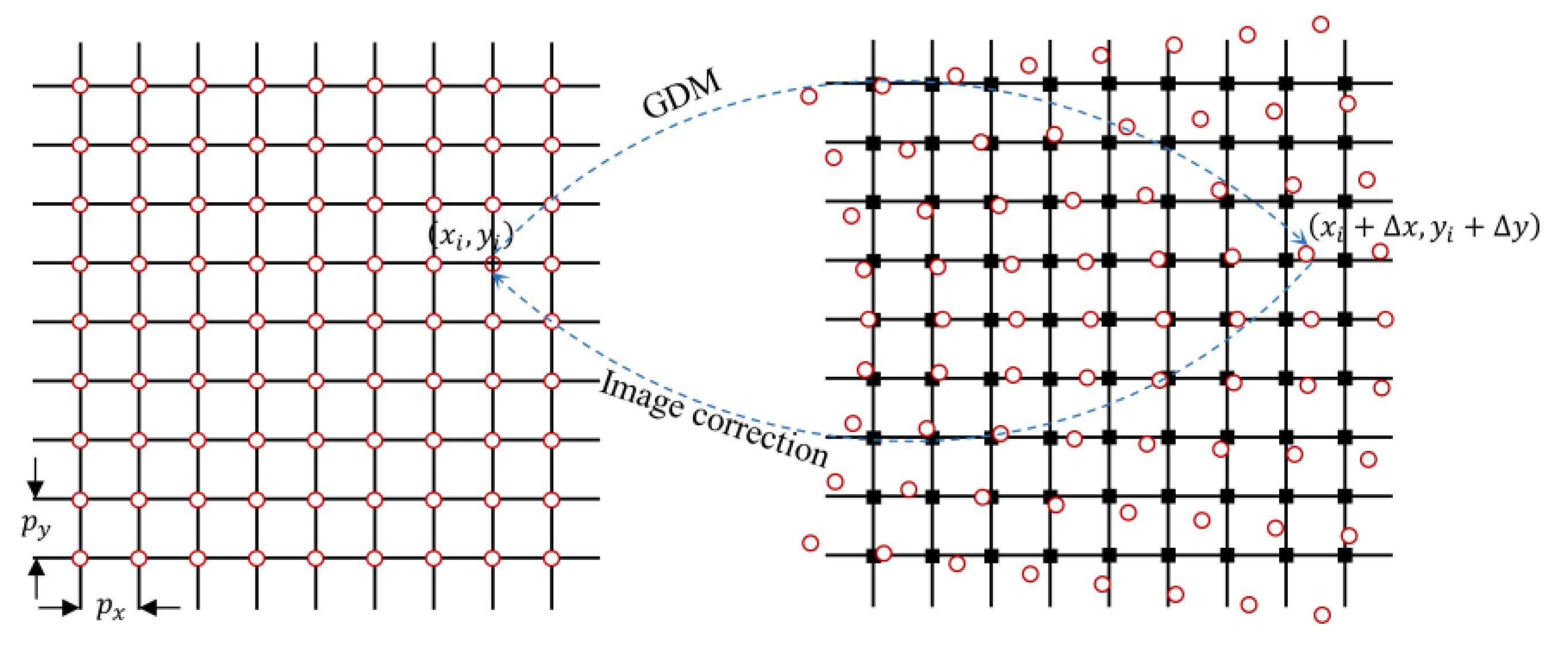
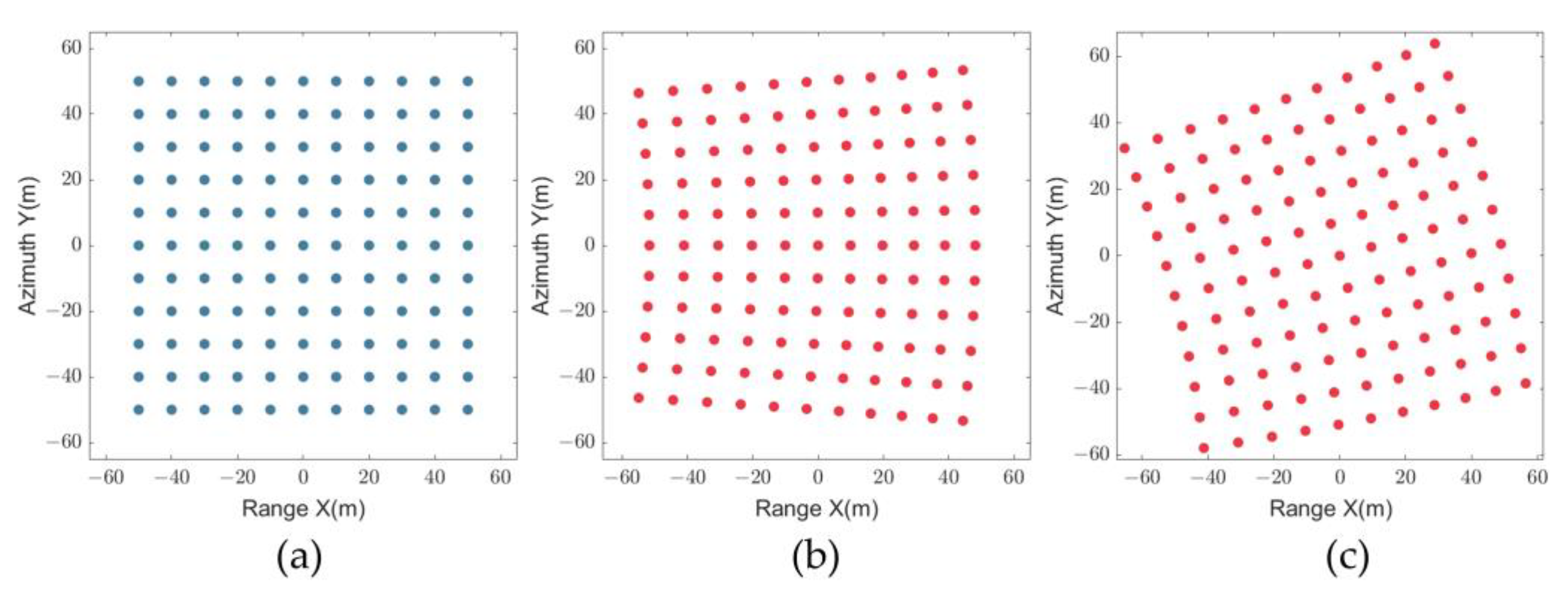
Geometric distortion correction can be accomplished by image domain interpolation, the key of which is to find the image coordinate positions of resampling points, and the GDM shown in (43) and (44) gives this relationship. The schematic diagram of geometric distortion correction is shown in
Figure 5. Since image rotation and distortion correction can be accomplished by one image domain, 2D interpolation, distortion correction, and coordinate system unification can be achieved simultaneously.
The quadratic terms of the difference distance are:
Additionally, the quadratic phase error is expressed in the form of the difference of the second-order derivatives of the difference distance:
The residual quadratic phase error is a two-dimensional spatial variable, so it is impossible to construct a filter to accurately compensate for the phase error at all points, which is the difficulty of compensating for the residual phase error. However, it is not necessary to compensate for it in all scenarios. In fact, it can be ignored if the phase error is less than a certain threshold during time-to-frequency conversion, and an approximate judgment formula is given in [
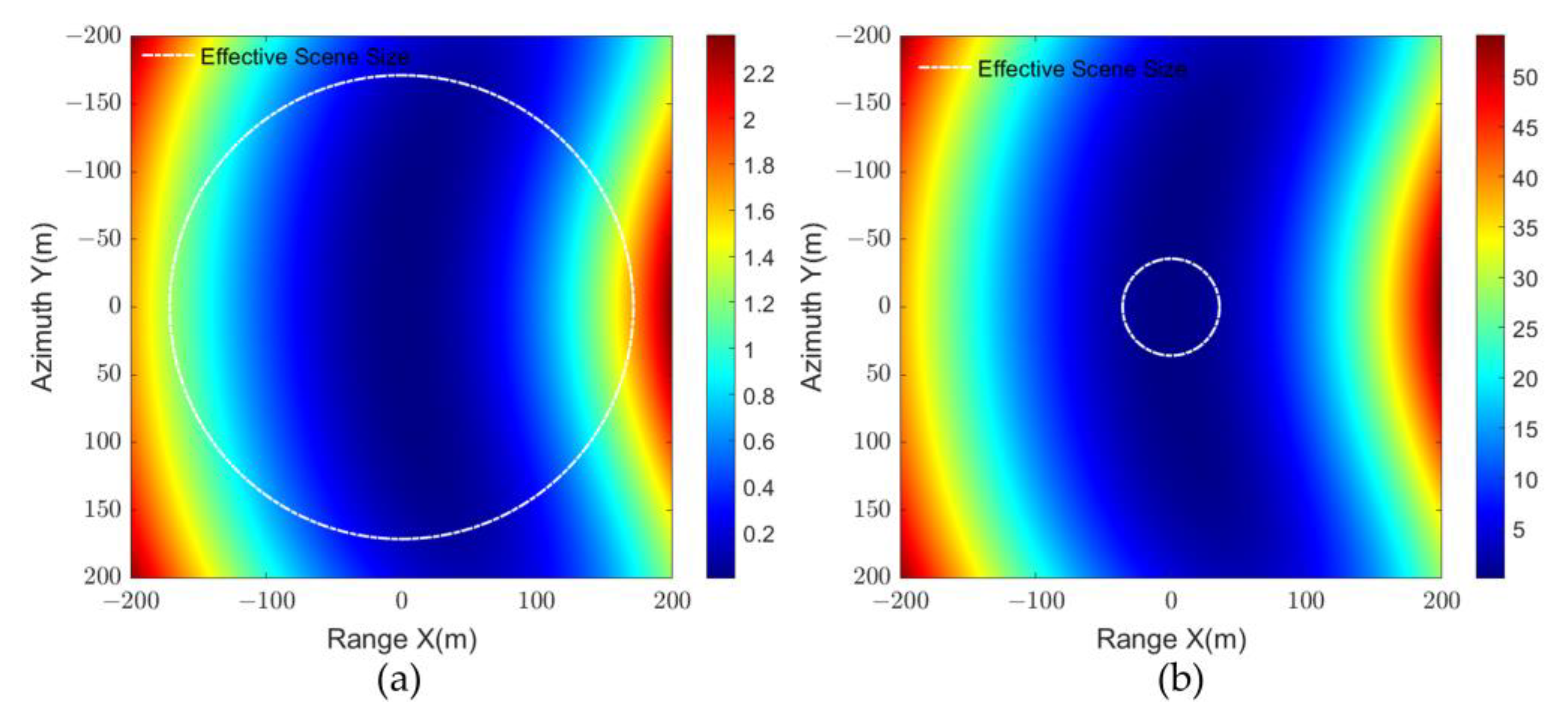
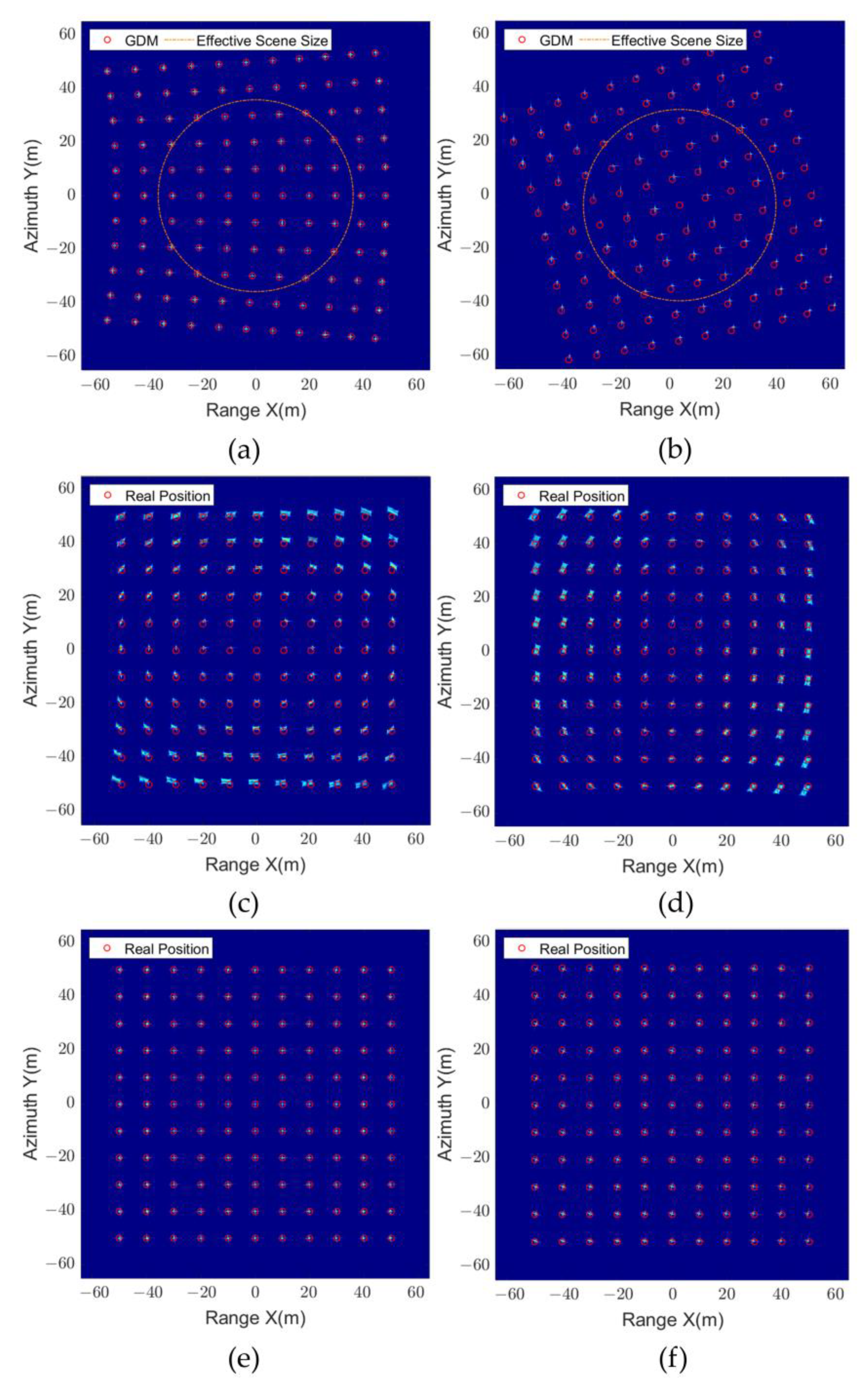
20]. Based on the threshold, the effective scene size is:
where
and
are the effective scene radius at thresholds of
and
, respectively, and
is the radar wavelength.
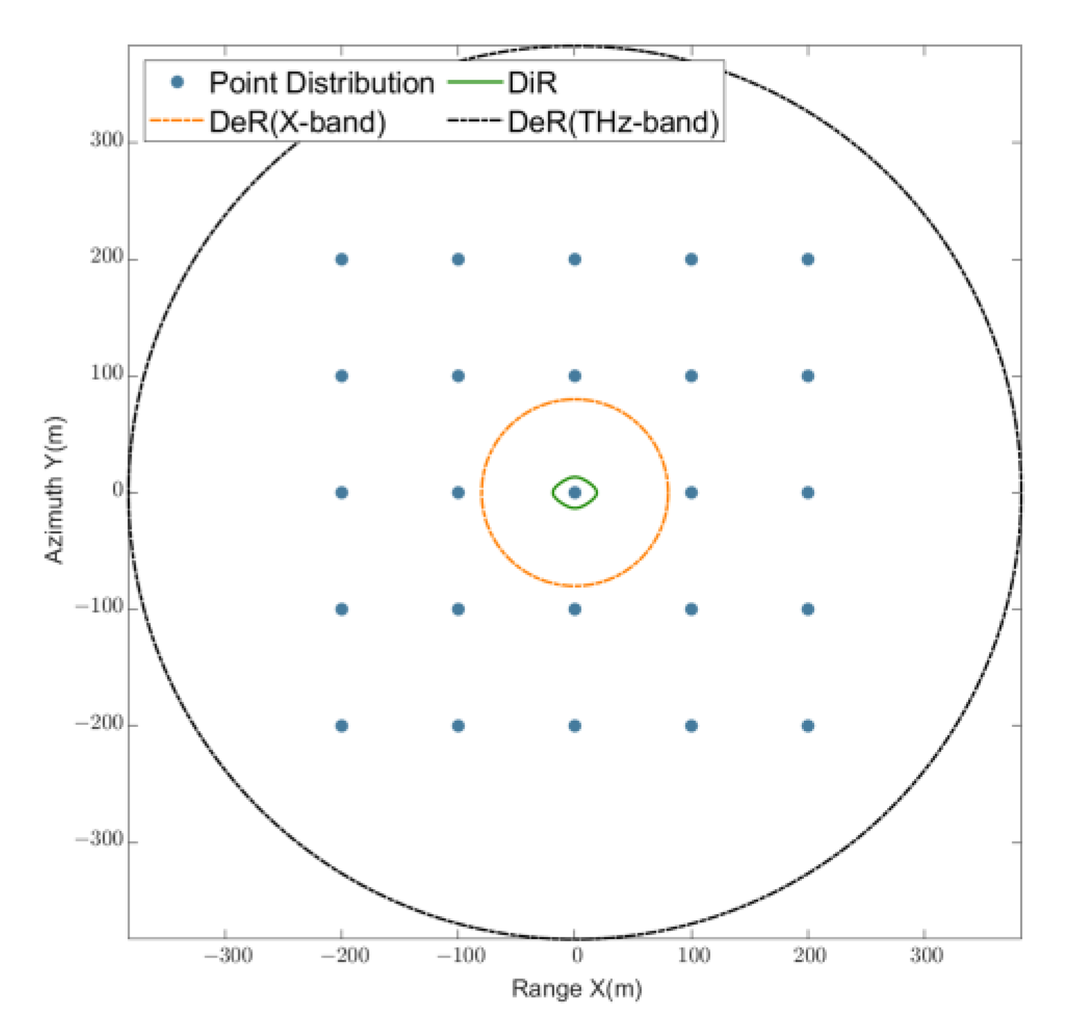
Similarly, the effect of image defocus can be ignored only within the defocus negligible region (DeR), which is defined as:
According to (46) and (50), the DiR and DeR at different frequencies can be calculated as shown in
Table 2, where the DiR is independent of the frequency and only related to the distance of the point target from the center point, both of which are 23.8 m.
In addition,
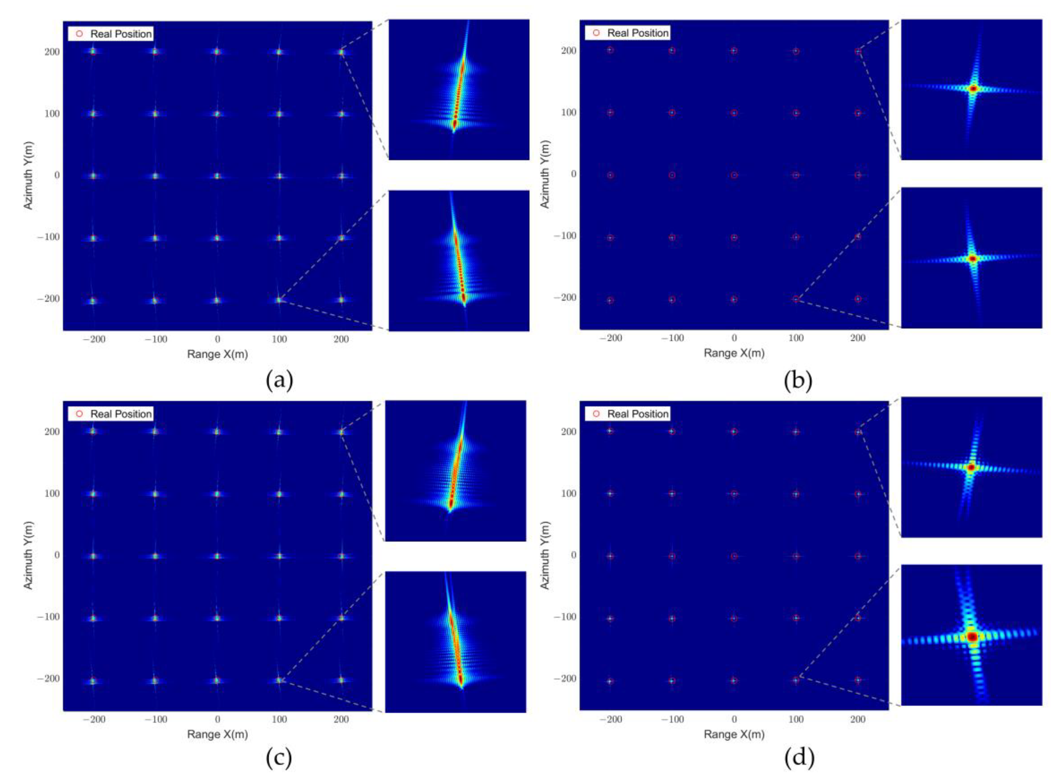
Figure 6 shows the residual quadratic phase error and the effective scene size at different wavebands, where the scene size is set to 200 m × 200 m. As shown in
Figure 6a,b, THz video SAR has a larger DeR of 171.3 m, while the X-band video SAR only has a DeR of 35.7 m. Generally, the scene size of video SAR is between 50 m and 150 m, so the effect of residual quadratic phase error can be ignored for THz video SAR, while the error must be corrected for X-band video SAR. This indicates that THz video SAR can ignore the effect of defocus in many cases, while it must be corrected for X-band video SAR.
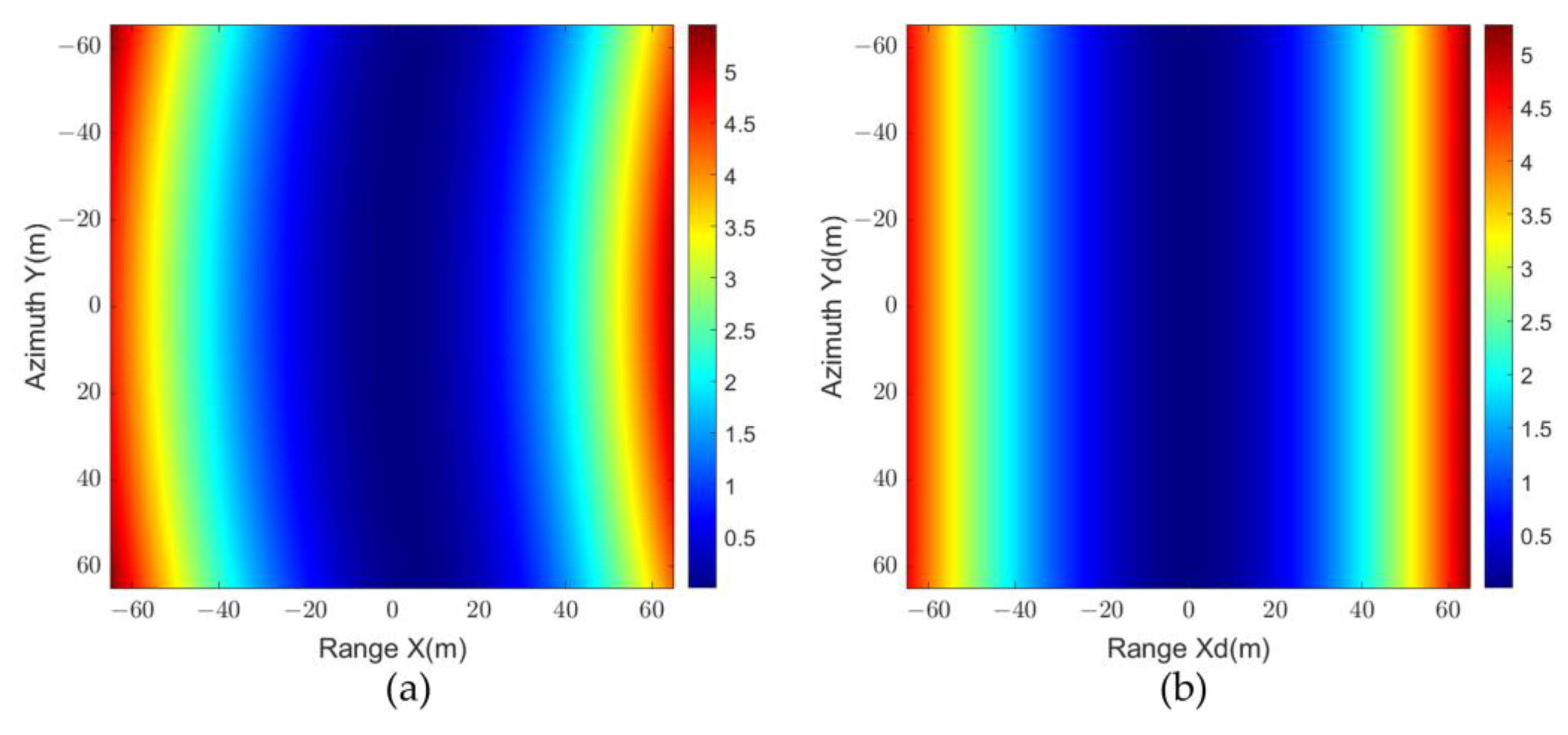
Figure 7 depicts the residual quadratic phase error in different coordinate systems under X-band video SAR with a scene size of 65 m, where
Figure 7a is shown in the actual coordinates
, and
Figure 7b is shown in the distorted coordinates
. It can be seen that the residual quadratic phase error is mainly a function of distance to the distorted coordinates
. Therefore, a correction for each range bin in the distorted coordinates can complete the compensation of the residual quadratic phase error.
Perform an azimuth FFT on the PFA image and perform a residual phase error compensation. The compensation function is:
The process of the compensation is:
where
and
denotes the azimuth FFT and azimuth IFFT, respectively. Then, a distortion-free video SAR image is obtained by applying geometric distortion correction to
.
3.3. Imaging Approach of GPPFA
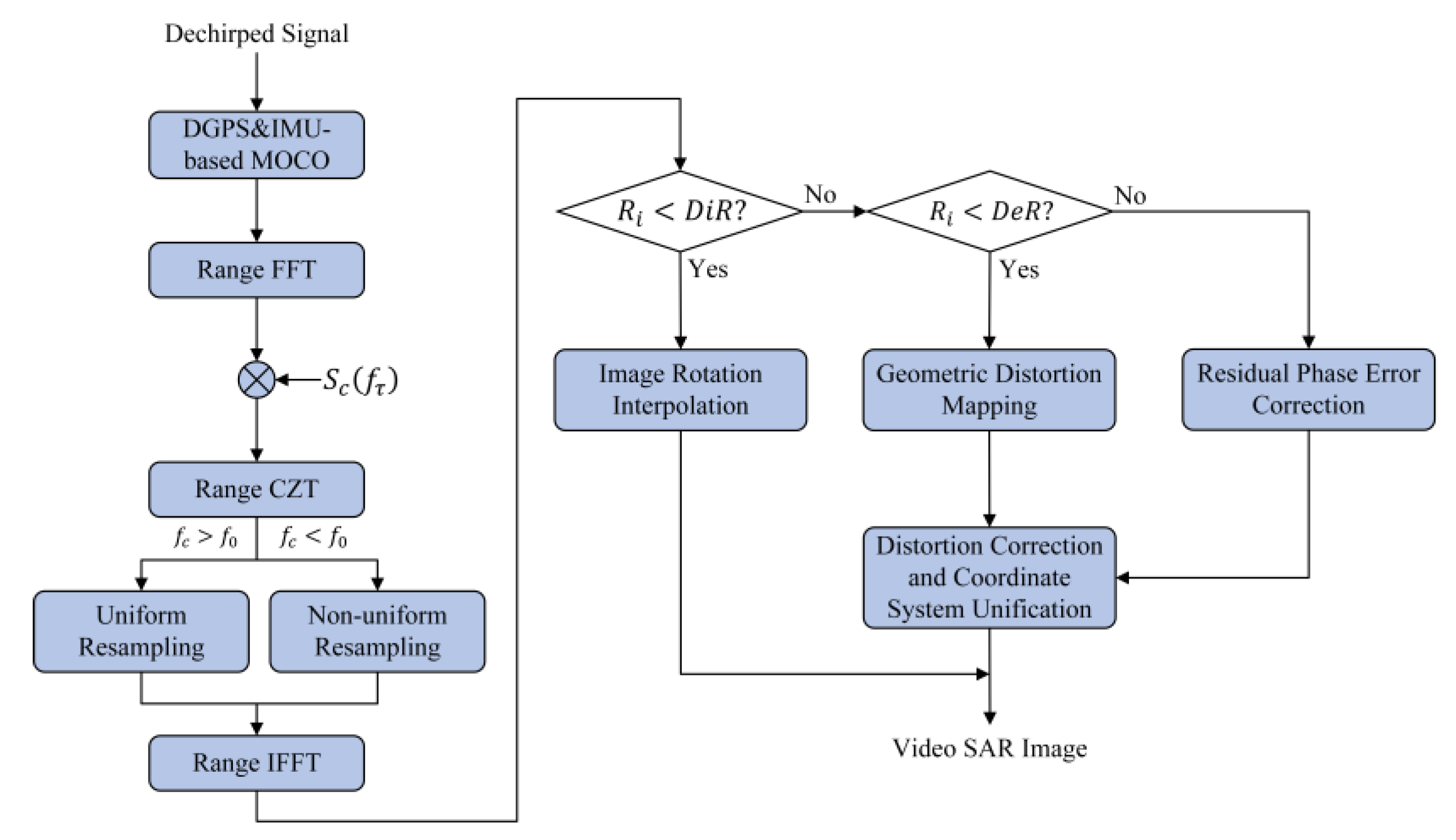
Based on the criteria obtained from the previous calculations, the flowchart of the proposed GPPFA can be described in
Figure 8.
Considering the possible trajectory deviation or platform vibration during the video SAR flight, which usually adversely affects the received SAR signal, a DGPS and IMU-based MOCO is applied before processing. After that, most of the motion errors are compensated, and the Map-drift algorithm (MD) [
52] or phase gradient autofocus algorithm (PGA) [
53] can be applied if the residual motion errors exist and affect the image.
Then, the range processing is based on range FFT, RVP compensation, and range CZT. For the possible wavefront curvature errors in the preliminary PFA image, the two criteria in (46) and (50) are chosen as the criteria to ensure the optimal processing flow in different scenarios.
For the case , only an image rotation is implemented. For the case , the distortion coordinate positions are calculated using the GDM, and the distortion correction and coordinate system unification are completed using an image domain 2D interpolation. For the case , the residual phase error compensation is required. The proposed GPPFA is capable of adapting to airborne video SAR imaging at any waveband, any slant range, and any scene size.
5. Conclusions
In this paper, a generalized persistent polar format algorithm (GPPFA) is proposed, which can meet the fast imaging of airborne video SAR in arbitrary waveband, arbitrary slant range, and scene size. Firstly, an airborne video SAR imaging model is established, and the high-resolution and high-frame rate characteristics and requirements of video SAR are analyzed. Then, the principle of CZT is introduced, and range resampling is completed based on CZT. For azimuth resampling, the critical of azimuth uniform resampling is analyzed, and the azimuth resampling of different waveband video SAR systems is completed based on azimuth CZT or interpolation, respectively. For the wavefront curvature error of PFA, the geometric distortion mapping of airborne video SAR in circular spotlight mode is derived, and a geometric distortion and image defocus correction method is proposed. GPPFA is capable of video SAR imaging at different wavebands, arbitrary scene sizes, and arbitrary flight trajectories. Point target and extended target experiments verify the accuracy, generality, and imaging efficiency of the proposed method. Although the proposed method is derived in circular spotlight mode, it can be applied to various working modes, such as linear spotlight mode and curve flight trajectories, as long as the platform position is accurately measured.
There are still some improvements to the proposed method. In reality, the THz video SAR platform is small and cannot carry high-precision DGPS AND IMU devices, and it is more sensitive to motion errors which may be introduced by airflow disturbance and attitude control. Therefore, the more accurate and efficient motion error compensation algorithm and its combination with the proposed method will be studied in the future to further improve the performance and generality of the algorithm.


