Article

Unsupervised Classification of Riverbed Types for Bathymetry Mapping in Shallow Rivers Using UAV-Based Hyperspectral Imagery

1
Institute of Construction and Environmental Engineering, Seoul National University, Seoul 08826, Republic of Korea
2
Department of Civil & Environmental Engineering, Dankook University, Yongin 16890, Republic of Korea
3
K-Water Institute, Daejeon 34350, Republic of Korea
*
Author to whom correspondence should be addressed.
Remote Sens. 2023, 15(11), 2803; https://doi.org/10.3390/rs15112803
Submission received: 16 March 2023 / Revised: 15 May 2023 / Accepted: 25 May 2023 / Published: 28 May 2023

Abstract

:
Passive remote sensing is a practical and widely used method for bathymetry mapping in shallow rivers. However, the accuracy of this approach is limited because of different riverbed types; therefore, it is important to classify the riverbed types for improving bathymetry mapping accuracy and providing useful information for fluvial systems. In this study, we proposed a Gaussian mixture model (GMM)-based clustering method that utilizes hyperspectral imagery to classify riverbed types without sampling the bed material. We evaluated the proposed method in two shallow streams with different bed mixture conditions: (i) sand and vegetation and (ii) sand and moss-covered sand. The results showed that the GMM method accurately identified the spectral variability caused by diverse riverbed materials, enabling the precise classification of riverbed types. Moreover, by combining the GMM method with optimal band ratio analysis, we observed a reduction in error for the bathymetry mapping results by approximately 0.05 to 0.07 m. While our proposed method exhibits potential applications in various river environments, further research is needed to validate its effectiveness in classifying more complex riverbed types and conditions. Overall, our study findings suggest that the GMM-based clustering method using hyperspectral imagery is a promising tool for improving bathymetry mapping accuracy and classifying riverbed types in shallow rivers.

1. Introduction

River bathymetry provides essential information for understanding the physical structure and dynamics of river ecosystems [1,2,3]. Furthermore, bathymetry data are essential for modeling river flow and sediment transport, which is vital for effective water resource management and flood risk prediction [4,5]. Additionally, riverbed material considerably influences water depth and flow as well as changes river morphology based on suspended sediments or the bed load, which are critical for aquatic habitats. However, obtaining both bathymetry data and information on riverbed substrates using conventional methods is time-consuming and labor-intensive, particularly for collecting high-resolution datasets. This challenge becomes even more crucial when mapping riverbed composition, primarily due to the dependence on riverbed material sampling at specific points [6,7]. Therefore, to overcome these limitations, remote sensing approaches are being widely used for river bathymetry estimation and bottom-type classification [8,9,10,11,12,13]. Remote sensing-based bathymetric surveys provide a more efficient and comprehensive means of characterizing fluvial systems over large areas and time frames [6]. With the use of unoccupied aerial vehicles (UAVs), bathymetric light detection and ranging (LiDAR) technology and structure-from-motion (SfM) photogrammetry have been widely used to analyze riverbed topography [4,14,15]. The bathymetric LiDAR technology is particularly effective for mapping riverbed topography using lasers to measure the water depth and riverbed shape. However, this approach is limited to considering spectral variability arising from various bed substrates and compositions in the water column since LiDAR uses only a single spectral range [16]. On the other hand, SfM photogrammetry can estimate the high-resolution 3D topography of riverbeds using images captured by UAVs. The most critical limitation of SfM photogrammetry for bathymetry mapping is its low water penetration, leading to lower accuracy than that of other methods [2].
Spectral-based approaches have also been widely used for bathymetry mapping using multispectral or hyperspectral data from satellites or UAVs [9,17,18]. These approaches inversely estimate the water depth based on the interaction between the signal absorbed by the light passing through the water column and the signal reflected from the bottom, as described by Lee et al. [19]. Recently, an empirical approach was used for bathymetry mapping by developing a regression equation between directly measured water depth and spectral bands. Legleiter et al. [9] proposed an Optimal Band Ratio Analysis (OBRA) algorithm to develop a linear regressor by determining the most relevant spectral band ratio with water depth. OBRA produces accurate results when specific conditions are met. In particular, it performs well when the river water is clear, the riverbed is relatively bright, and depths are shallow because, in this case, the dominant signal component is the bottom-reflected radiance [20]. Despite this limitation, OBRA has been successfully adopted in various riverine areas and has demonstrated great feasibility [8,21,22,23,24]. Additionally, this method has been advanced into a nonlinear functional form, making it suitable for application in rivers with more optical complexity [11].
Studies on the determination of riverbed characteristics via remote sensing have been conducted less frequently than bathymetric measurements [6,19]. Legleiter et al. [19] initially evaluated the potential for riverbed classification in shallow and clear rivers using a combination of reflectance magnitude and spectral shape indices. However, they also highlighted a limitation in determining the complex relationship between water depth and bottom reflectance under various sediment and algal bottom conditions. This complex relationship can be explained using a simplified radiative transfer equation for shallow waters from Lee et al. [18], as expressed in Equation (1):
R r s ( λ ) = R ( λ ) ( 1 e K ( λ ) H ) + ρ b π e K ( λ ) H
where R r s is the remote sensing reflectance, λ is the wavelength, R is the reflectance of infinitely deep water, H is the water depth, K(λ) is the attenuation coefficient, and ρ b is the bottom albedo determined according to the riverbed material. This equation suggests that the bottom reflectance, which is the second term on the right-hand side, exponentially decreases as water depth increases, with the maximum value determined from ρ b . Therefore, the relationship between the water depth and riverbed substrate is often conflicting. Furthermore, deep water makes it challenging to classify riverbed composition, whereas diverse bottom types make it difficult to estimate water depth from spectral data. To develop spectral regressors for water depth, true values can be collected by using practical sensors, such as real-time kinematic (RTK)-GPS and an Acoustic Doppler Current Profiler (ADCP), which allow uncomplicated in situ measurements of water depth [25,26]. However, investigating the characteristics of riverbed materials requires the collection of samples from the river bottom, which becomes increasingly challenging, particularly when it is covered with vegetation, moss, or algae. Overall, accurately characterizing fluvial systems requires a multifaceted approach that accounts for the complex interplay between water depth and riverbed type.
In this study, an unsupervised classification technique using clustering was used to classify riverbed types. The primary advantage of this method is that it eliminates the requirement to sample specific riverbed materials and enables the mapping of riverbed types across a wide area. Moreover, the accuracy of hyperspectral image (HSI)-based bathymetry, using the OBRA approach, was then evaluated under varying riverbed conditions, including vegetated, sand, and moss-covered bottoms. We aimed to assess the effectiveness of using the clustering technique and OBRA method to simultaneously measure riverbed types and bathymetry under complex riverbed conditions. The evaluation was conducted under two different shallow and clear river water conditions to determine the accuracy of the method under such conditions.

2. Materials and Methods

2.1. Field Survey

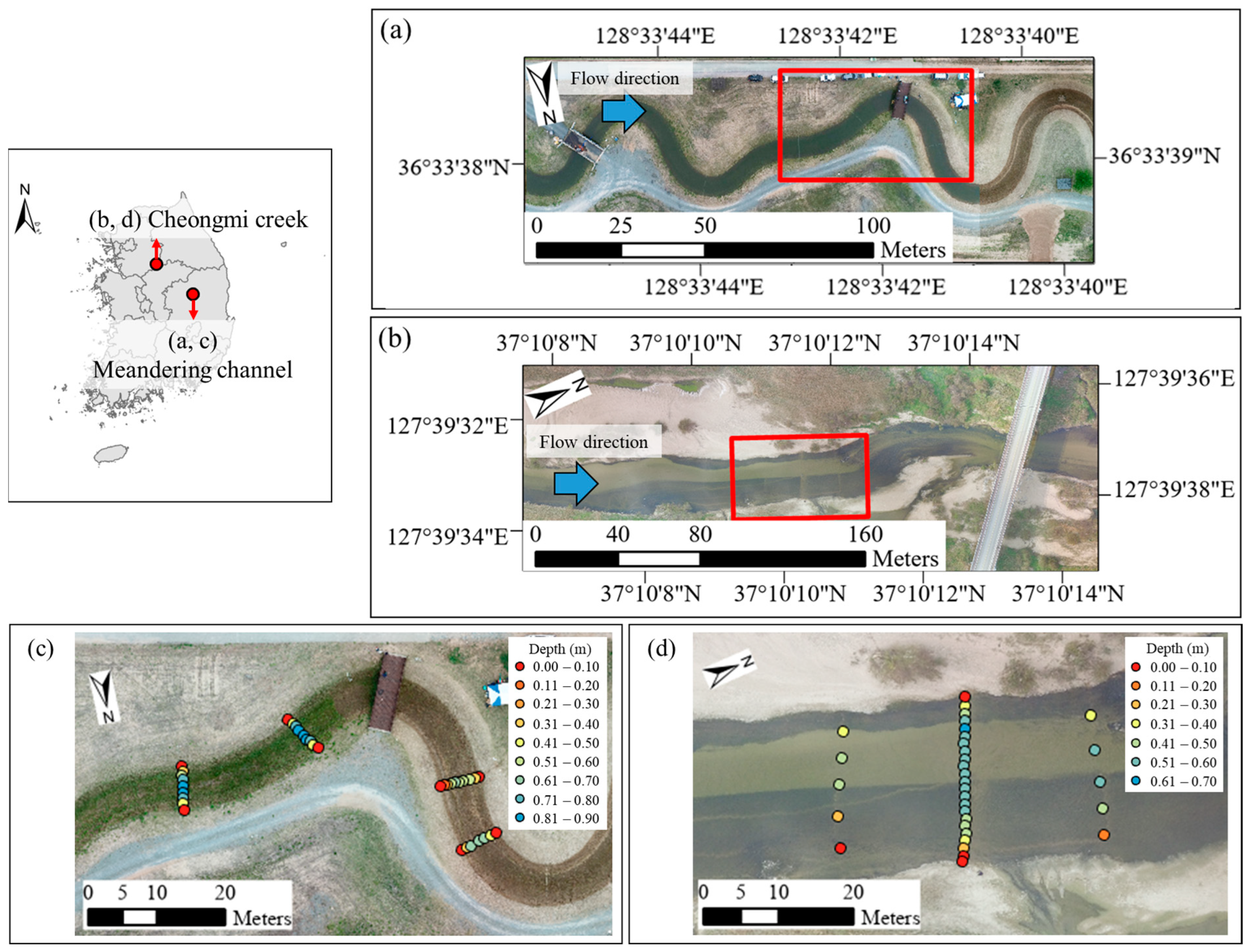
2.1.1. Study Site and In Situ Measurements

This study was conducted at two sites featuring shallow streams with mixed bed types. Case 1 was a meandering channel (Figure 1a,c) located at the River Experiment Center (REC) of the Korea Institute of Civil Engineering and Building Technology. The REC is situated in Andong, South Korea, and sources water from the nearby Nakdong River [24]. The meandering channel, which is an artificially created field-scale experimental channel, is 682 m long, 11 m wide, and has a maximum controllable depth of 2 m with a 1:800 slope. The bed material of this channel comprises vegetation and sand, which naturally forms abundant vegetation during spring and summer; the vegetation degenerates during autumn and winter. As the experiment was conducted on 28 April 2021, corresponding to the spring season, vegetation grew throughout the channel, as shown in Figure 1c.
To conduct the experiments on the two different riverbed materials (vegetation and sand), weeding was performed downstream past the wooden bridge to longitudinally separate the channel into sand and vegetated bed areas, as shown in Figure 2a. The vegetation height was 0.05–0.10 m in the vegetated area, whereas the particle size of the bed material was approximately 1.11 mm in the sand area. The flow rate supplied during the experiment was 2.41 m3/s, which was regulated by controlling the water pump in the pump room [27]. The vegetation area of the upper reach of the channel had an average width of 5.76 m; the stream formed in such a way that the channel width widened to 6.26 m while the water depth became shallower in the downstream reach. During the field survey, the in situ water depth and horizontal position were measured using an RTK global positioning system (RTK-GPS; Sokkia GRX1, Sokkia, Japan) in four sections, comprising two lines in the vegetated area and two lines in the sand area (Figure 1c). The RTK-GPS has an accuracy of 10 mm + 1 ppm in the horizontal stationary survey and 15 mm + 1 ppm in the vertical stationary survey [28]. For the bathymetric survey using this equipment, position information was recorded at specific intervals from the water surface, i.e., from the left bank to the right bank, after installing a tagline with 1 m increments in the lateral direction of the river. The endpoint of both river sides was set as the water surface, and the riverbed altitude measured underwater was subtracted from the water surface altitude to calculate the water depth. Based on this process, 35 points of water depth to the riverbed were measured, ranging from 0 to 0.88 m in the vegetated area and from 0 to 0.64 m in the sand area.
The experiments in Case 2 were conducted at Cheongmi Creek, located in Yeoju, South Korea (Figure 1). The field survey was conducted on 8 November 2022, during the dry season, with a stream flow rate of 3.22 m3/s, as described in Table 1. The riverbed materials were bifurcated according to the flow direction, with bright sand distributed on the left side of the stream and dark moss covering the sand bed on the right side, as depicted in the close-view photograph in Figure 2b. In the upstream reach of the study area, the tributary inflow induced a shallower zone owing to sediment deposition in the field near the river conference, as shown in Figure 2b. Moreover, underwater wood caused irregular areas in the downstream reach, where the moss was scattered on the sand bed. This heterogeneity in bed material could lead to significant spectral variability owing to the different spectral characteristics of each bed material. Furthermore, this spectral variability arising owing to stream bed differences could weaken the accuracy of the hyperspectral estimator for water depth while also providing information for the classification of bed materials.
For in situ water depth measurements, 33 points of water depth data were collected at three cross-sections, as shown in Figure 1d. In these sections, the maximum water depth was 0.63 m near the left bank on the sand bed, whereas the maximum water depth was shallower (0.54 m) near the right bank on the moss-covered bed. The particle size distribution of the site was confirmed in the Cheongmi Creek Basic Plan Report [29], and the median particle size was found to be 2.75 mm, as listed in Table 1; this was larger than that of coarse sand.

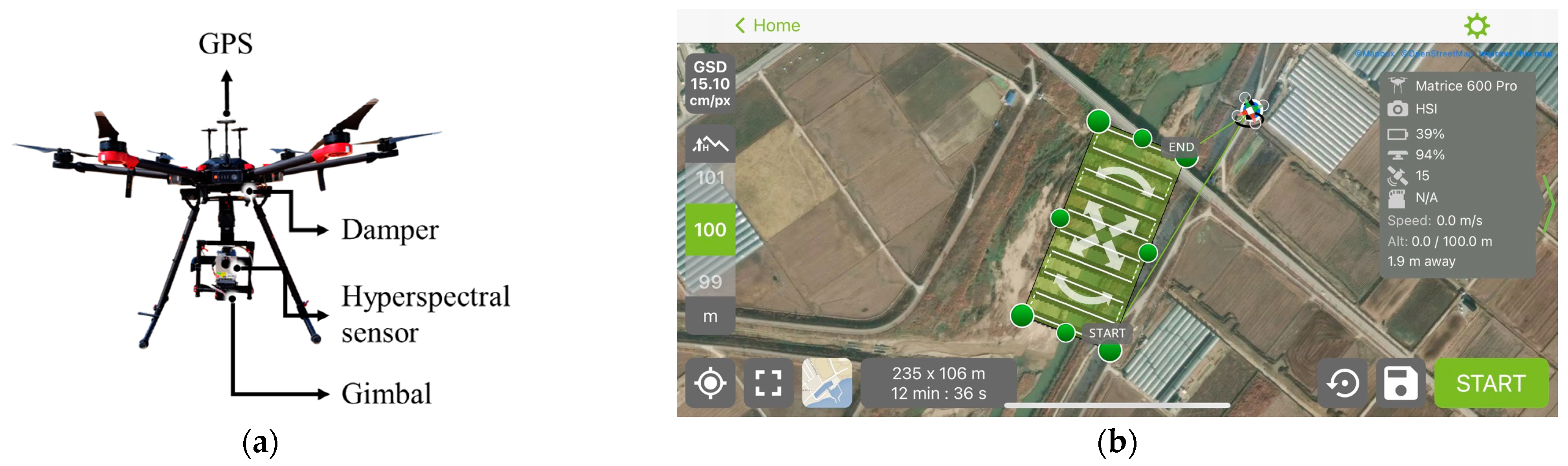
2.1.2. Hyperspectral Data Acquisition

Figure 3 demonstrates the drone system used for acquiring HSIs. To capture the full range of the visible to near-infrared (NIR) spectrum, a hyperspectral sensor (MicroHSI 410 SHARK, Corning Inc., Corning, NY, USA) was used [30]. This sensor can obtain data within the wavelength range of 400–1000 nm. The spectral resolution of this sensor is 4 nm, and it can acquire 150 spectral bands within the collectable wavelength range. The maximum frame rate is 300 Hz, with a field of view of 29.5°. The imaging method used was push broom-type line scanning, which captures spectral information in a linear space rather than in a plane when capturing a frame at a specific location. The sensor was equipped with an Inertial Navigation System containing a Global Navigation Satellite System receiver and a microelectromechanical system-based Inertial Measurement Unit, thereby enabling the acquisition of precise information on position and attitude. The sensor, including the lens, was compact and lightweight, with dimensions of 13.6 cm × 8.7 cm × 7.0 cm and a weight of 0.68 kg, facilitating its installation on a drone for operational use. In the present study, we first mounted the sensor on the DJI Ronin-MX gimbal (DJI, Shenzhen, China; Figure 3a) to adjust the shooting angle and then installed it on the Matrice 600 Pro drone (DJI, China) with a hovering accuracy of ±0.5 m vertically and ±1.5 m horizontally. Flight missions were set using drone flight software (Pix4Dcapture version 4.13; Figure 3b) to control the drone and gimbal during the flight missions. The hyperspectral imaging system employed in the present study has been used to determine various river properties, including suspended sediments, bathymetry, and algal blooms, by mounting it onto a drone [24,27,31,32,33,34].
Before field surveys, we calibrated the hyperspectral camera using a lens cap as a dark reference and a 25.4 cm × 25.4 cm Labsphere spectralon as a white reference before the drone flight [35]. In addition, microHSI 410 SHARK processed and stored the hyperspectral data as raw HSIs with digital numbers and calibrated HSIs. The calibrated HSIs were processed via dark subtraction and non-uniformity correction (NUC), with the resulting units being W/m2/sr/µm as radiance [30]. NUC is a scene-based correction that adjusts both the radiance conversion and inhomogeneity of individual pixels in an HSI [36,37]. Therefore, we used NUC-processed HSIs by converting radiance values to reflectance. For this radiometric correction, calibration tarps reflecting 12%, 36%, 56%, and 84% of the incident radiation were used. Standard reflectance values were obtained before each experiment by placing the calibration tarps on a flat ground. After the field surveys, we used the collected standard reflectance values for radiometric correction using the empirical line correction in ENVI version 5.6 software [38]. To obtain HSIs covering a precise area, the processed HSIs were clipped to remove unnecessary areas and retain only the necessary ones. Subsequently, geometric calibration was performed to georeference the image and assign coordinates, followed by image registration to combine the segmented images into one image. For hyperspectral analysis of the riverbed classification and bathymetry estimation, we used 100 spectral bands between 450 and 850 nm to eliminate redundant wavelengths sensitive to interference, such as surface turbulence and wave facets, and to prevent poor reflectance retrieval from NUC in the relatively dark NIR region [27,36,39,40].
In Case 1, we operated the drone at an altitude of 50 m to obtain HSIs with a resolution of approximately 0.04 m/pixel, covering an area of approximately 181 m × 55 m. Kwon et al. [26] conducted hyperspectral imaging surveys in the same study area and collected HSIs from a specific lateral line by hovering a drone to accurately estimate the suspended sediment concentration under certain bed conditions. In contrast, we collected HSIs over a wide area, including sand and vegetated bed areas (Figure 1c) by moving the drone under clear water conditions. In Case 2 at Cheongmi Creek, the drone’s altitude was set at 100 m, resulting in a coverage length of approximately 53 m for the HSIs, with a resolution of approximately 0.077 m/pixel, and covering an area of approximately 235 m × 106 m.

2.2. Hyperspectral Clustering

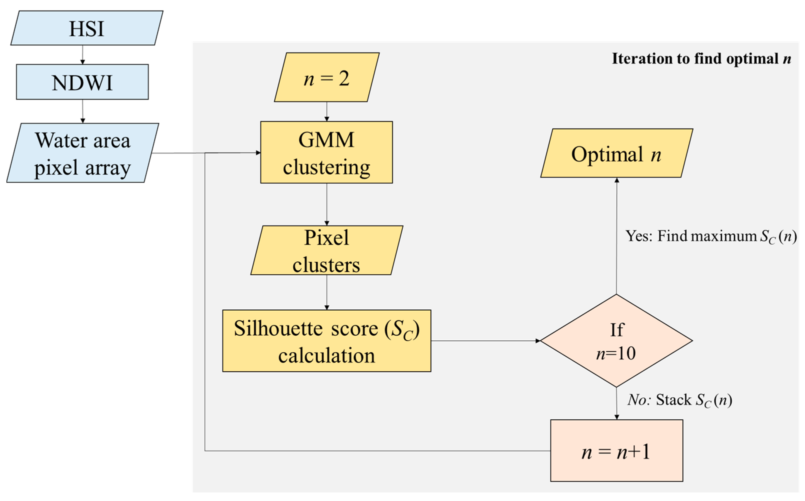
2.2.1. Gaussian Mixture Model (GMM)

GMM is a stochastic clustering method that uses a mixture of Gaussian distributions to statistically split non-Gaussian distributions into several clusters [26,33]. Compared with heuristic-based clustering methods such as k-means and hierarchical clustering, GMM offers several advantages. First, it accounts for variance, allowing the clustering of datasets with stretched structures. Second, the fitted probability density function (PDF) provides the probability of belonging to each cluster. Complicated water column attenuation and bottom albedo induce spectral variability, as expressed in Equation (1), and the GMM is advantageous for managing complex hyperspectral data owing to its ability to handle stretched structure datasets to model non-Gaussian distributions [34].
In particular, the GMM fits the multivariate dataset using a weighted combination of heterogeneous Gaussian distributions. The fitted mixture of Gaussian distributions represents the PDF of the entire dataset as a non-Gaussian distribution. Subsequently, the clusters can be split into a single Gaussian distribution to ensure the statistical uniformity of each cluster.
P x = k = 1 K ω k N k ( x μ k , Σ k ) ,
where K is the number of clusters, ω k denotes the mixture coefficient ranging from 0 to 1, and 1 K ω k = 1 . N k is a single Gaussian distribution of the kth cluster with mean ( μ k ) and covariance matrix ( Σ k ). Each split Gaussian distribution of the kth cluster is expressed as
N k ( x μ k , Σ k ) = 1 2 π d 2 Σ k 1 / 2 e x p ( 1 2 x μ k T Σ 1 x μ k ) ,
where d is the matrix dimension, T is the transpose of the matrix, and Σ is the determinant of Σ . The parameters that need to be estimated in GMM are denoted as θ = π , μ , Σ , where π, μ , and Σ are equivalent to π 1 , , π k , μ 1 , , μ k , and Σ 1 , , Σ k , respectively. The log-likelihood of θ can be defined as
L θ x = i = 1 n l n { k = 1 K ω k N k ( x μ k , Σ k ) } .
To estimate θ, we used the expectation maximization (EM) algorithm to maximize the log-likelihood in Equation (4). The EM algorithm initializes each parameter and evaluates the log-likelihood using Equation (4). In the expectation step, we estimated the probability of each data point belonging to the kth cluster from the responsibility (γ) using the current θ value in Equation (5).
γ k x = ω k N ( x μ k , Σ k ) m = 1 K ω m N ( x μ m , Σ m ) .
In the maximization step, the values of θ were updated via repeated estimation according to the responsibility. These steps were iterated until the θ values reached the maximum likelihood in Equation (4) [41].

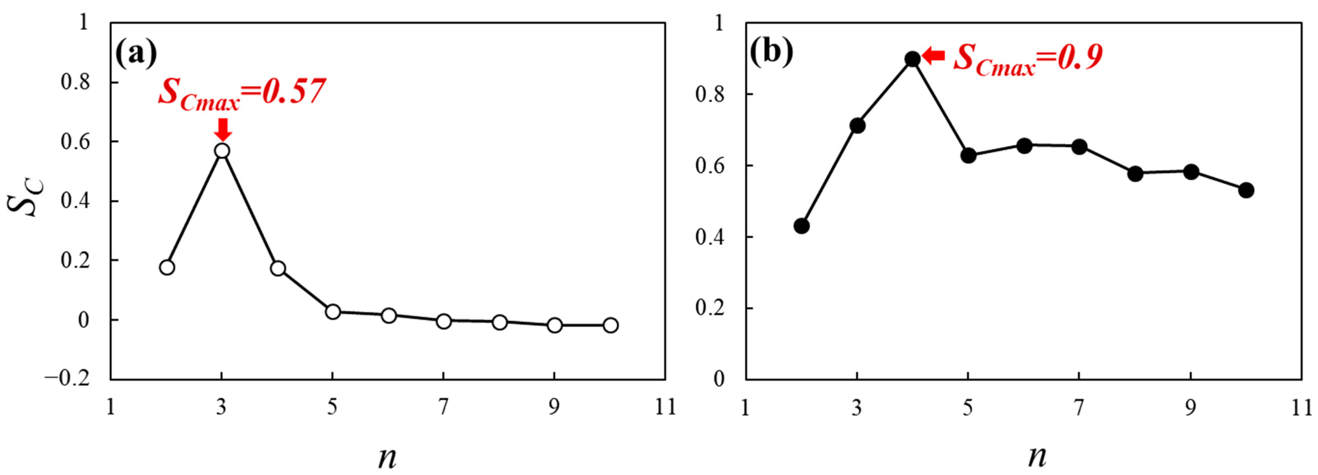
2.2.2. Selection of Optimal Clusters

When clustering hyperspectral data, the number of clusters critically affects their quality [27]. We used the silhouette coefficient (SC) to assess the validity of the clusters from the GMM based on the number of clusters. This metric measures the effectiveness of cluster separation by evaluating the distance between each cluster [42]. The general silhouette value (S) for object i can be expressed as
S ( i ) = b i a ( i ) m a x { a i , b ( i ) } ,
where a(i) represents the degree of similarity within a cluster, defined as the average distance of object i from all other points in the same cluster, and b(i) is the distance from object i to the data of the nearest cluster. S ranges from −1 to 1, with values closer to 1 indicating better cluster validity [i.e., a(i) < b(i)]. Finally, SC can be calculated using the mean S(i) from the entire dataset.
In the present study, we first extracted water area pixels by selecting the pixels with positive values for the normalized difference water index (NDWI) using the green (535 nm) and NIR (820 nm) bands [43]. NDWI is widely used to classify water areas and is expressed as follows [43,44,45]:
N D W I = R G r e e n R ( N I R ) R G r e e n + R ( N I R ) .
After the selection process, we calculated the Sc value by increasing the number of clusters from 2 to 10. This was achieved by targeting the water area pixel array in the HSI. Subsequently, we evaluated the number of clusters with the maximum value, as shown in Figure 4, to determine the optimal number of clusters for GMM clustering. Finally, the determined clusters for all pixels in the HSI indicate different riverbed types based on their spectral characteristics. Although this method does not precisely analyze riverbed properties, it can provide an estimated classification of the riverbed types based on their spectral characteristics. To identify the spectral characteristics of each riverbed cluster, we used the OBRA approach, which is described in the next section.

2.3. OBRA

OBRA is the most widely used hyperspectral analysis method to locate relevant spectral bands and develop specific regressors for river bathymetry [8,10,22,23,46]. In OBRA, the spectral characteristics of the water depth can be characterized based on the band ratio between the reflectance (R) of two specific bands, as indicated by Equation (1). In the present study, we characterized the spectral features associated with water depth using the log-transformed version of Equation (8), where λ1 and λ2 represent the particular wavelengths of the two bands.
X = l n R ( λ 1 ) R ( λ 2 ) .
The OBRA approach estimates the coefficient of determination (R2) of the regression equation for the in situ-measured water depth and estimated water depth from the band ratio using all possible band combinations. R2 indicates the calibration agreement of the regression equation [46,47]. In addition, the optimal band ratio was determined by identifying the combination with the highest R2. This process can be visualized as an R2 map with wavelengths λ1 and λ2 [9]. The final regression equation for bathymetry was built using the band pair with the highest R2. The regression equation can be set in various forms, such as linear, quadratic, exponential, and power-law equations [11].
The OBRA approach is practical and provides an explicit relationship between the water depth and band ratio. Previous studies have demonstrated that this approach is accurate for bathymetry in clear and shallow rivers, where the relationship between water depth and the band ratio is highly linear [8,9,10,21,22]. However, the accuracy of the depth estimation is critically limited under high turbidity and deep water depth conditions [10]. In this study, we used linear regression for OBRA because the background water quality was relatively clear and the water depth was shallow, as indicated by the low turbidity in Figure 1 and Figure 2.

3. Results and Discussion

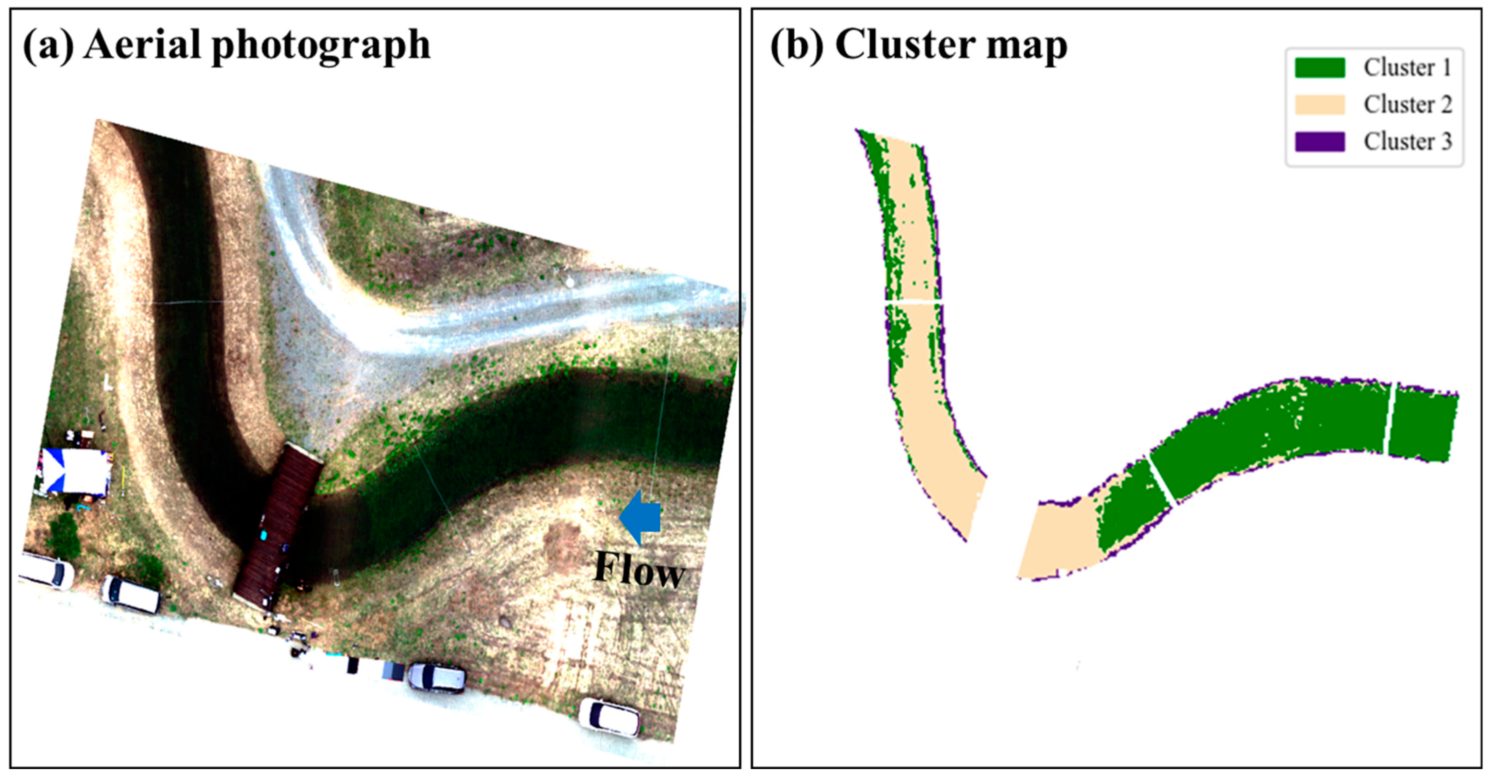
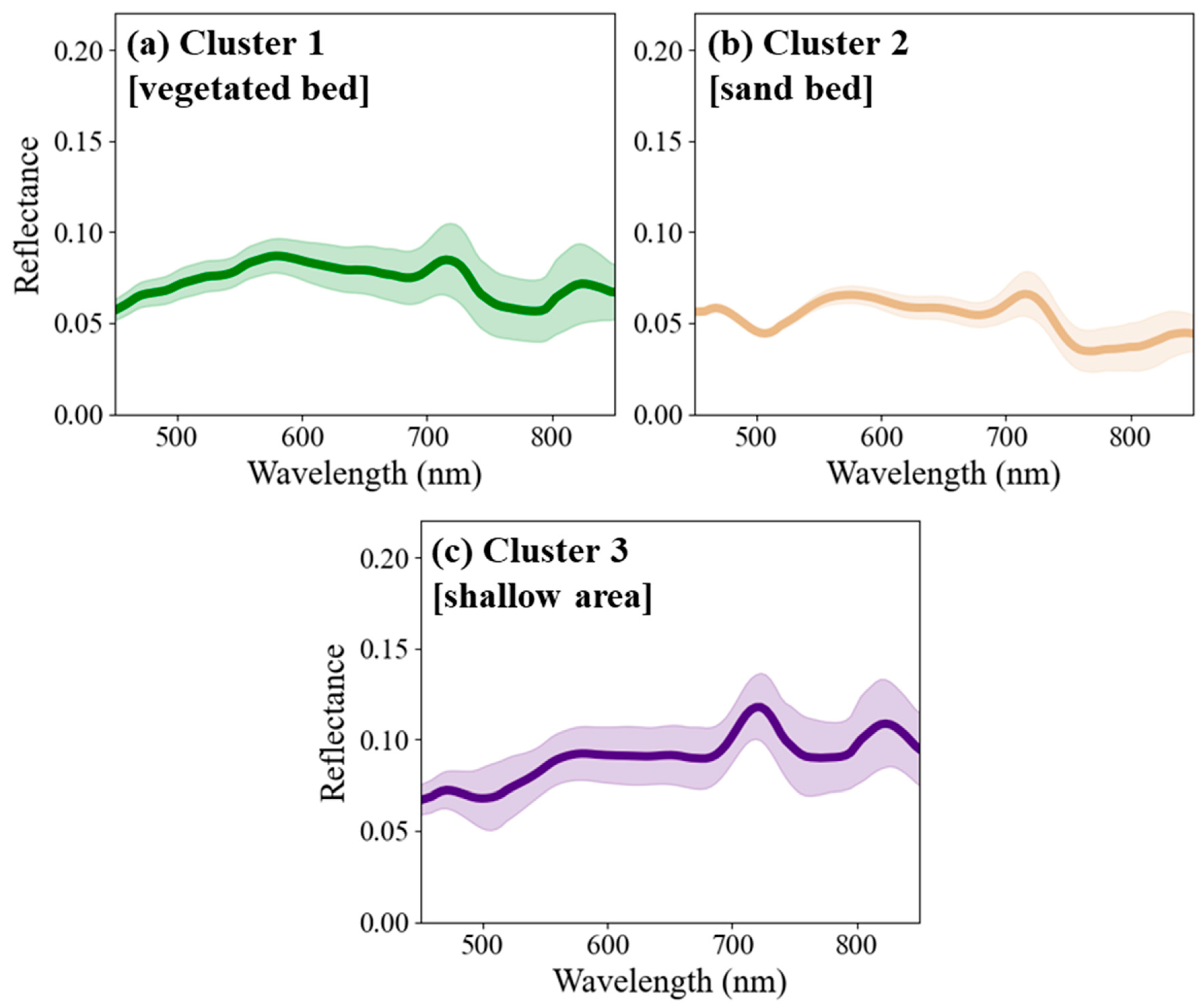
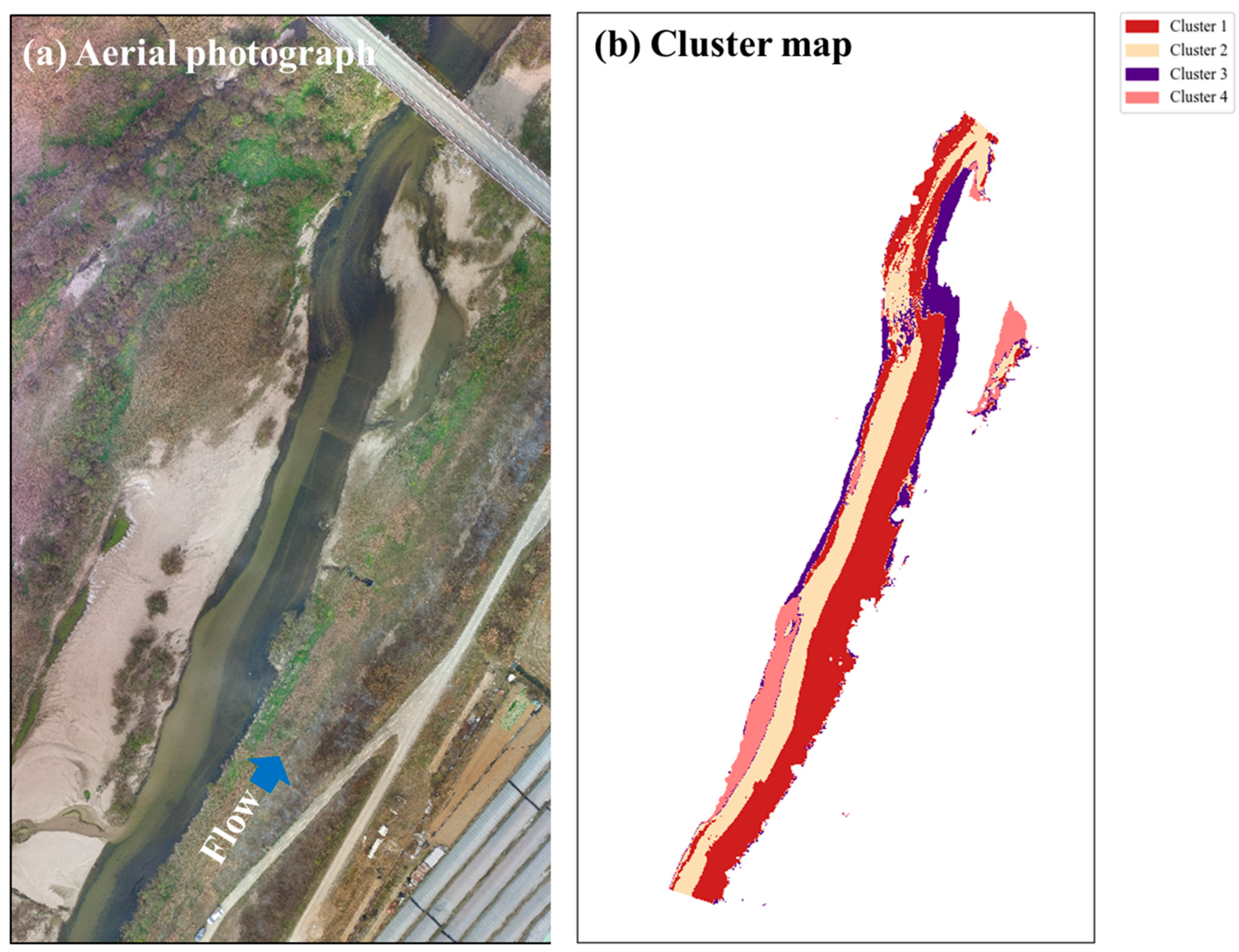
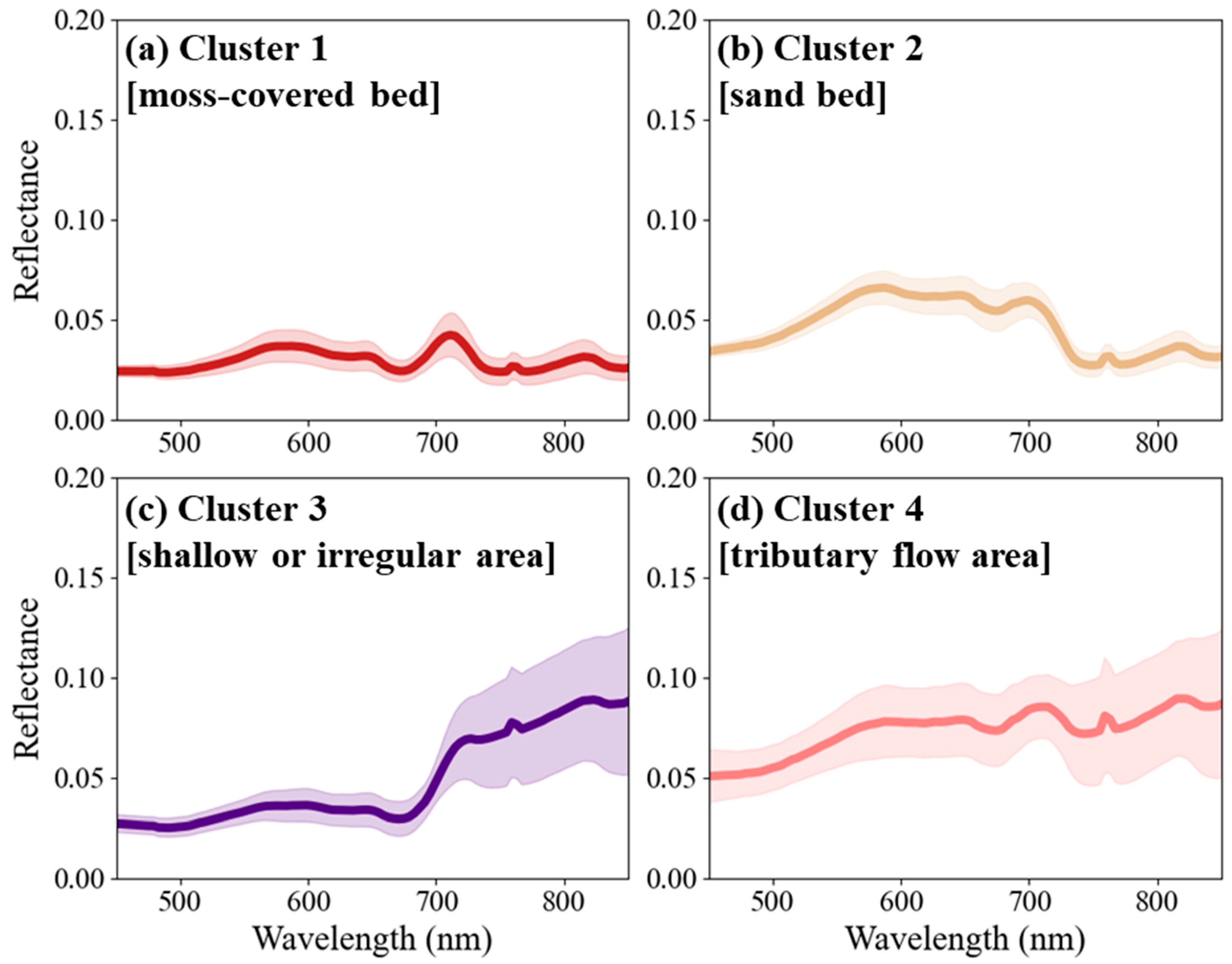
3.1. Classification of the Riverbed Type

To identify the optimal number of clusters, we calculated the SC for all water pixels while varying the number of clusters from 2 to 10, as illustrated in Figure 5. The number of clusters corresponding to the highest SC was selected as the optimal value. For Case 1, SC peaked at three clusters and decreased gradually when the number of clusters was higher than three. When the number of clusters was higher than five, SC became negative. The maximum SC value was 0.57, which surpassed the minimum threshold of 0.5, indicating a well-classified cluster [48]. For Case 2, the optimal number of clusters was estimated to be 4, with an SC value of 0.9. Notably, the SC value was maintained above 0.5, even when the number of clusters increased. This result suggests that Case 2, a natural river, is more complex than Case 1, an artificial channel with multiple components and dominant bottom material. Nevertheless, the SC values at the optimal points indicate that Case 2 was more effectively classified than Case 1. Despite the presence of vegetation, the sand signal was detected in areas with relatively low vegetation density in Case 1.
Figure 6 shows an aerial photograph and cluster map with the optimal clusters in Case 1. The cluster map revealed distinct classification results, with vegetation and sand areas represented by Clusters 1 and 2, respectively. Cluster 3 was the highly shallow zones along the waterline. Notably, the boundary between the vegetation and sand areas upstream of the bridge was well divided compared with the aerial photograph. However, some pixels in the vegetated area were also assigned to Cluster 2, indicating that the sand signal obscured the vegetation signals, leading to a decrease in the SC value. Similarly, some pixels in the sand area were classified as Cluster 1 in the downstream reach. Although vegetation was removed from this section, some remaining vegetation appeared to have been captured.
Figure 7 shows that each cluster had distinct spectral characteristics. Cluster 1, which mainly classified the vegetation area, exhibited a relatively high standard deviation in the reflectance spectrum. This finding is consistent with that of a previous study that reported the movement of vegetation by flow as a spectral characteristic that can be detected particularly in shallow rivers [27]. Additionally, reflectance values in the visible wavelength range (500–700 nm) were higher in Cluster 1 than in Cluster 2, consistent with the brightness of both areas in the RGB image (Figure 5a). In contrast, the reflectance spectrum of Cluster 2 exhibited low reflectance and standard deviation in the visible range. Typically, in the NIR region (λ > 750 nm), the water column absorbs most of the light, resulting in a low reflectance. However, in this study, the water depth was < 1 m; therefore, the overall reflectance in the NIR region reflected from the bottom was relatively high in Clusters 1 and 3. Cluster 3 (the water area boundary) exhibited higher reflectance values and standard deviations than Clusters 1 and 2 owing to the shallowness of the water column, causing a weak attenuation effect, and the turbulence near the wall.
In Case 2, the maximum SC value in Cheongmi Creek was as high as 0.9, resulting in a cluster map that showed precise segmentation of the river area, consistent with the RGB image presented in Figure 8. The two dominant clusters identified in this case corresponded to sand and moss-covered bed areas. In addition to these two clusters, the very shallow area near the boundary of the river was classified as Cluster 3, although most of this area was covered with moss, as shown in the RGB image (Figure 2b). Similarly, the sand bed area in the near field after the confluence was identified as Cluster 4. Cluster 3 also included an irregular area with a wooden obstacle in the downstream reach, as shown in Figure 2b. Near this obstacle, the water surface was irregular owing to turbulence or vortex shedding behind the obstacle [49]. Such irregularities can hinder the transmission of light through the water column. Cluster 4 was affected by the deposition of sediments flowing from the tributary, resulting in shallower water depths. The spectral characteristics of the differences in sand properties between the tributary and the main stream were also likely to have been reflected. Additionally, in the sand area, dunes developed on the riverbed (Figure 2b), which could have influenced the spectral characteristics of the sand and contributed to the irregular riverbed shape.
The reflectance spectrum of each cluster in Case 2 exhibited different spectral characteristics corresponding to riverbed characteristics (Figure 9). The shapes of the reflectance spectra in Cases 1 and 2 were markedly different. In the visible wavelength range, Cluster 2 had a higher reflectance value than Cluster 1 and exhibited a peak at approximately 600 nm, whereas Cluster 1 had a low reflectance in the visible range, with a peak at approximately 700 nm. This result suggests that the moss absorbed light in the visible wavelength range, although the wavelength near the NIR range (λ > 750 nm) was maintained compared with Cluster 2. Clusters 3 and 4 exhibited higher reflectance in the NIR region than the dominant bed classes (Clusters 1 and 2). This result was due to the surface reflection resulting from the turbulence near the water surface and the low attenuation of light due to the shallowness of the water (H < 0.2 m), which is consistent with that of the shallow area (Cluster 3) observed in Case 1. In particular, the substantial increase in reflectance above 700 nm in Cluster 3 of Case 2 could have been induced by the roughness of the water surface owing to the presence of underwater trees [39].

3.2. Retrievals of Water Depth According to Riverbed Type

We investigated the spectral characteristics of different riverbed types classified based on hyperspectral clustering and their potential contribution to improving bathymetry estimations using the OBRA approach. Figure 10a–c depict the OBRA results for Case 1 with and without hyperspectral clustering. When the OBRA approach was applied separately to the dominant riverbed types (moss-covered bed and sand), which were clustered using GMM, there was an increase of 6% and 5% in R2 for Clusters 1 and 2, respectively. Additionally, compared to OBRA without clustering, the RMSE decreased by 0.06 m and 0.07 m for the respective clusters. The effective wavelength range also changed when hyperspectral clustering was applied. As shown in Figure 10b,c, the vegetated and sand beds showed a wider range of effective wavelengths (R2 > 0.8) than OBRA without clustering (Figure 10a). This result demonstrates that hyperspectral clustering can reduce the spectral variability of the dataset by spectrally dividing it according to the riverbed type [27]. The optimal wavelengths of both clusters were green (533–590 nm) and red edge (698–713 nm), whereas only OBRA revealed that blue (458–523 nm) and red (650–690 nm) were the optimal wavelengths. Clusters 1 and 2 showed similarly effective wavelengths in OBRA even in the vegetated bed, and the sand under the vegetation was identical to the sand area. These signals from sand were detected between the vegetation, as shown in Figure 5. However, the regression equations for the water depth were different because of their distinct spectral characteristics, as shown in Figure 10e. The gradient of the linear regressor was higher for the vegetated bed than for the sandy bed. In addition, the linearity of each regressor from both clusters was more substantial than that of the regressor without clustering (Figure 10d), and the residuals of the regression also decreased, as shown in Figure 10e.
For Case 2, the application of hyperspectral clustering had a more significant effect on OBRA. In particular, the moss-covered and sand beds exhibited distinct differences in their effective wavelength ranges, as shown in Figure 11b,c. While the effective range of Cluster 2, with an R2 higher than 0.8, was widely and clearly distributed, moss demonstrated an overall decrease in R2 and a relatively high R2 with water depth only in a specific wavelength range near the red edge (767.13 and 709.06 nm) (Figure 11b). This result suggests that the spectral characteristics of moss make detection challenging and obscure the original riverbed characteristics. Notably, this finding suggests that a high spectral resolution is required to detect the water depth under the moss-covered bed, as evidenced by a specific effective wavelength range from OBRA.
Regarding accuracy (R2 and RMSE), the implementation of OBRA without clustering in Case 2 was less accurate than that in Case 1 (Figure 11a,d). This is because the more complex components in the riverbed of natural rivers lead to more substantial spectral variability, which limits the performance of OBRA. However, the implementation of OBRA with clustering produced a high R2 of 0.80 and 0.88 for Clusters 1 and 2, respectively, as depicted in Figure 11b. Additionally, the different spectral characteristics of the riverbeds classified into the two clusters are represented by distinct equations in Figure 11c,e.
A comparison of the mapping results between the original OBRA and GMM–OBRA in both cases showed a more apparent difference in the performance of the two approaches. For bathymetry mapping using GMM–OBRA in Case 1, the equations in Figure 10e were applied to pixels within Clusters 1 and 2. Cluster 3, which corresponded to the river boundary, was mapped using the equation of the dominant bottom cluster closest to the corresponding pixels. Susequently, a significant difference was observed in the sand area near the bridge. In particular, as shown in Figure 12c, compared with GMM–OBRA, the original OBRA approach tended to produce depth estimates that were lower near the upstream weeding area of the bridge and higher near the downstream area of the bridge.
In Case 2, based on the clustering results in Figure 8, mapping was conducted using two regression equations for sand and moss-covered bed areas. The irregular areas and inflow of tributaries caused significant noise in the spectra of Clusters 3 and 4; however, the beds themselves were close to the moss-covered and sand beds, respectively; thus, the equations derived from Clusters 1 and 2 were applied to Clusters 3 and 4, respectively. As shown in Figure 13, the topography of Case 2 was complex. In particular, a relatively deep water depth of > 0.5 m was observed in the sand bed area, whereas a water depth of < 0.5 m was mainly observed in the moss-covered bed area. In this regard, the difference in estimated H between both methods differed based on the riverbed type. Compared with GMM–OBRA, the original OBRA underestimated H in the sand bed area (Clusters 2 and 4) but overestimated H in the moss-covered bed area (Clusters 1 and 3). Therefore, the difference map in the two study cases demonstrates that the results of hyperspectral imagery-based bathymetry substantially vary depending on the bottom characteristics. In this respect, hyperspectral clustering enhanced the performance of OBRA for bathymetry by separating the spatial area according to spectral characteristics.

3.3. Discussions and Future Studies

Although hyperspectral remote sensing has considerably contributed to river bathymetry mapping by providing detailed spectral information, many limitations remain because of spectral variability in water environments [10,11,40,50,51]. We performed the present study under shallow and clear water conditions; however, poor water quality, high turbidity, and deep water generally decrease measurement performance. Such confounding factors typically hinder the intrinsic signals of the riverbed; therefore, both riverbed type classification and bathymetry mapping are challenging. In addition, our approach was subjective since the evaluation of the classification result of the river substrate relied on comparing the spectral difference between each cluster with riverbed images. Nevertheless, we proposed a possible solution to improve the performance of hyperspectral bathymetry mapping for one of the dominant confounding factors: spectral variability caused by different riverbed types. In particular, the most important result of the present study was that the accuracy of HSI-based bathymetry mapping increased in both cases where the classification of approximate bottom types was performed solely using imagery without in situ measurements using RTK-GPS or ADCP.
In future studies, combining hyperspectral clustering with advanced regressors (i.e., nonlinear regression, machine learning, and deep learning) may improve the performance of hyperspectral bathymetry mapping under more complex conditions. Gwon et al. [40] measured the depth of shallow rivers under varying suspended sediment-laden flow conditions using machine learning. By combining the method for classifying bottom types proposed in the present study with the method that can be used under high turbidity conditions, we can expand the applicability under various conditions of suspended sediments and water quality.
A limitation in deep waters is one of the critical points of remote sensing-based depth measurement techniques. As shown in Eq 1, the bottom reflectance decreases exponentially with increasing water depth. This phenomenon indicates that detecting and distinguishing spectral signals from different bottom types becomes ambiguous and challenging in deep waters. The available depth for classifying the river substrate directly depends on the measurable depth achieved through the hyperspectral retrieval of bathymetry. Legleiter et al. [11] reported that in clear water, green LiDAR can measure up to a depth of approximately 2 m, whereas the hyperspectral approach can measure up to a depth of approximately 3.8 m. However, if the diversity of bottom types can be considered using the method proposed in the present study, the heterogeneity of the bottom reflectance can be minimized for the water depth estimator. Consequently, this approach has the potential to increase the maximum measurable depth. In such an application, using machine learning or deep learning models will further improve performance because they can reflect a higher number of spectral bands, as suggested by Kwon et al. [27]. However, to build a robust machine learning model, it is important to develop a sampling strategy that can reflect various spectral characteristics [10]. If the data size is small, the model tends to be biased, with high accuracy only in areas where in situ data are available. Therefore, in future studies, we need to obtain additional data than those used in each case of this study.

4. Conclusions

The GMM-based hyperspectral clustering approach presented in this study exhibits superior performance in classifying riverbeds based on bottom material, without the need for in situ measurements or bed material sampling. This riverbed classification method helps comprehend the spectral variability caused by diverse riverbed materials in the two cases studied. The clustering results allow the development of a regression equation that can accurately separate the riverbed material and improve water depth measurements using OBRA. The main findings of this study are as follows:
  • After the optimal number of clusters was determined using SC, Case 2 (natural river) was found to exhibit a higher level of separability among each cluster than Case 1 (field-scale channel), which included only vegetation and sand. Nevertheless, in complex areas arising from underwater trees or very shallow water depths (H < 0.1 m), additional clusters that were distinct from the dominant riverbed clusters were formed.
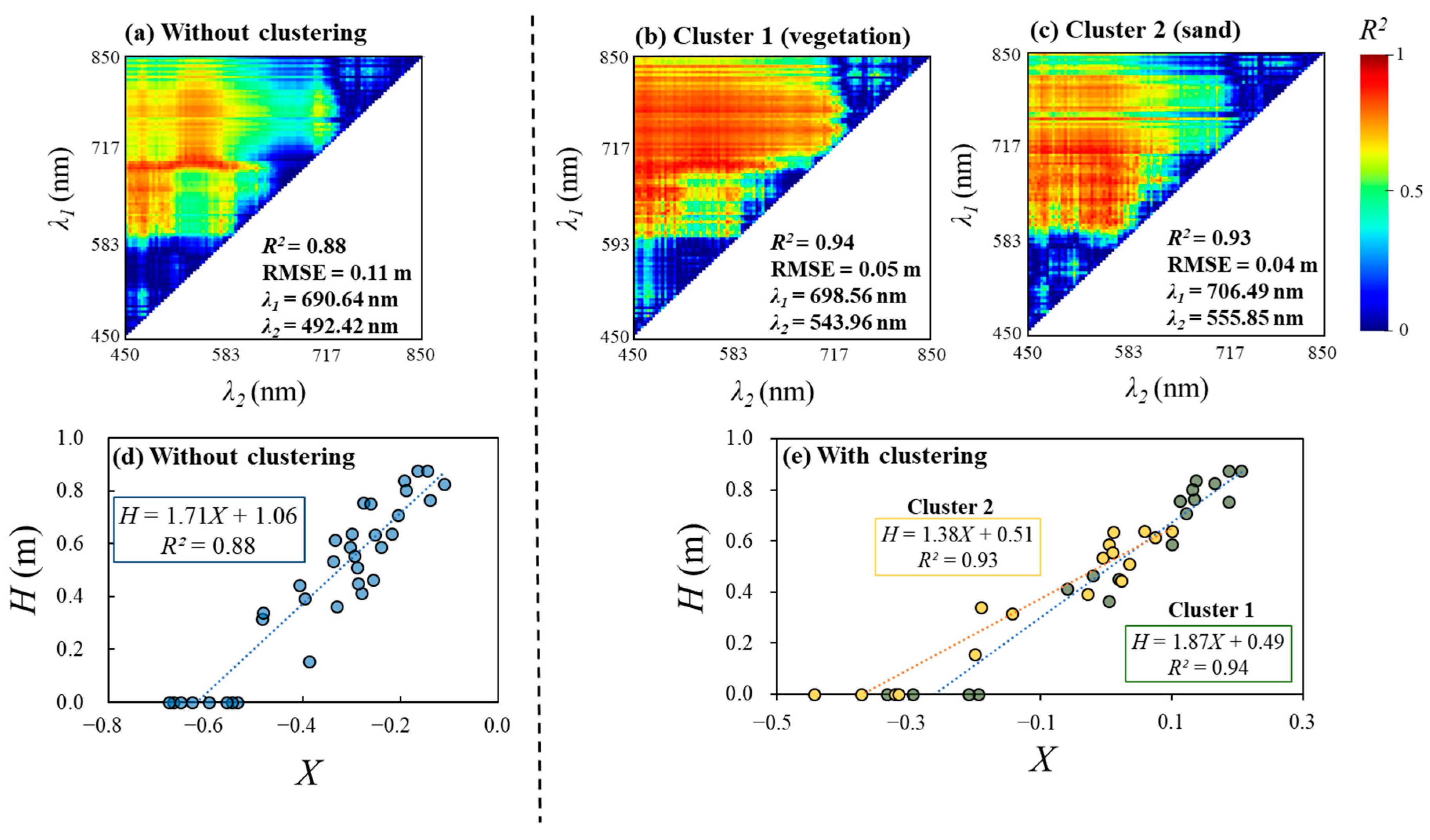
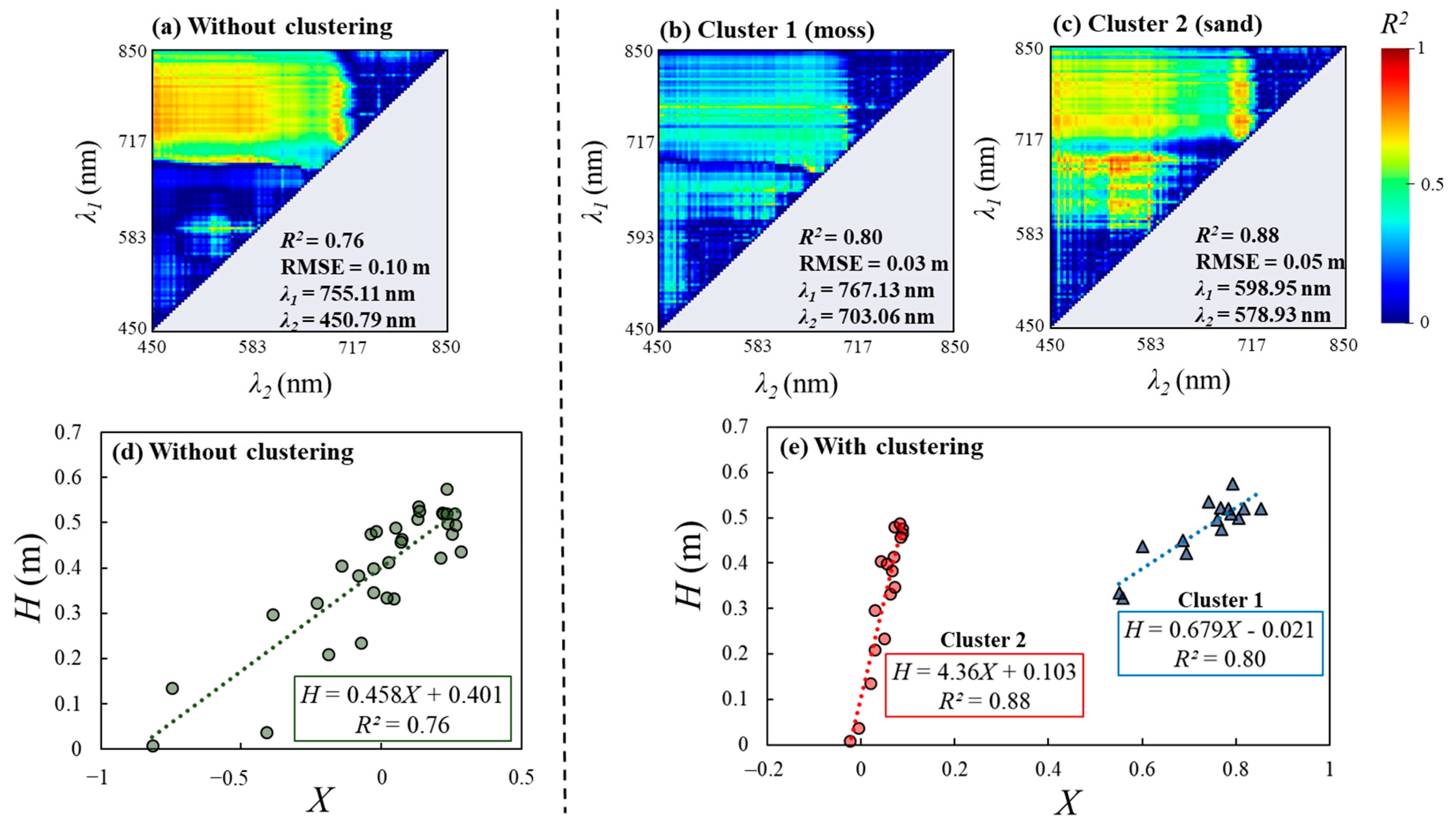
  • GMM statistically classified each cluster into areas with distinct spectra in two cases with complex bed conditions: (i) sand and vegetation and (ii) sand and moss-covered bed conditions. Each cluster exhibited a different equation form and an effective wavelength range from OBRA.
  • In particular, for Case 2, the moss-covered riverbed exhibited high linearity with water depth, having an R2 of 0.8 only within a specific and narrow wavelength range. This implies that the classification of such a riverbed using GMM with spectrally low-resolution HSIs and a limited range of wavelengths can be challenging.
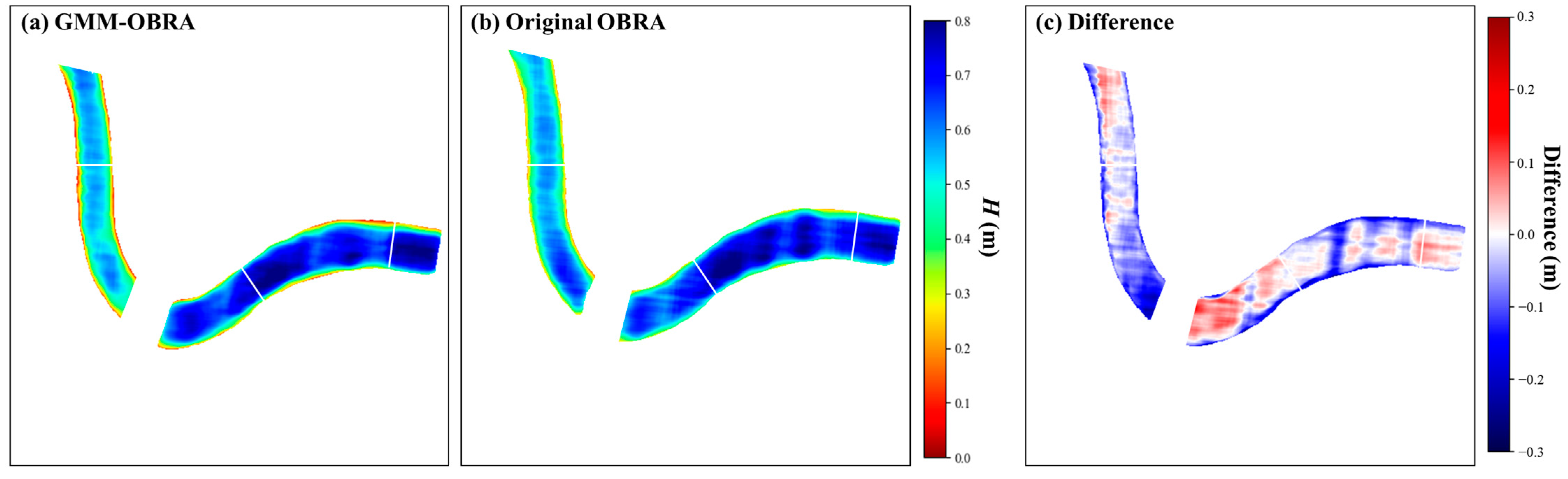
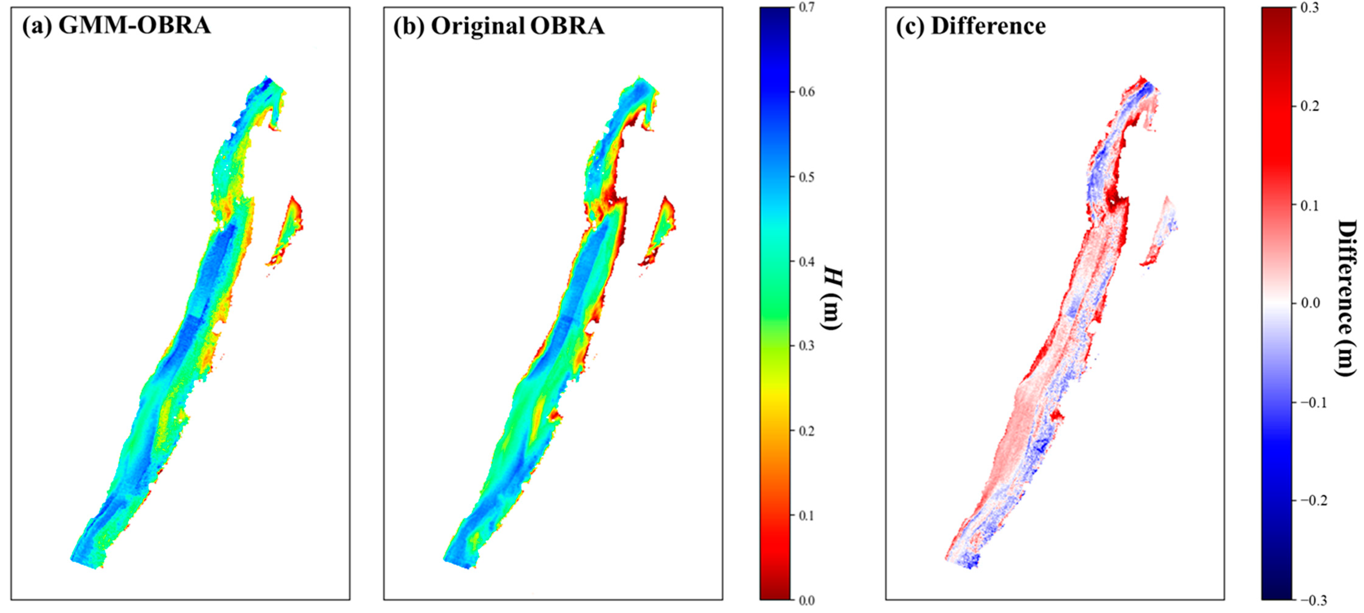
  • A considerable discrepancy was observed in the bathymetry mapping results between GMM–OBRA and the original OBRA. The original OBRA tended to either overestimate or underestimate certain clusters compared with GMM–OBRA. On the other hand, GMM–OBRA provided a means for accurately identifying riverbed types, thereby facilitating precise bathymetry mapping using straightforward linear regressors from OBRA.
Despite the substantial improvements in bathymetry estimation and riverbed type classification in this study, future studies should investigate more diverse riverbed types and conditions to validate the effectiveness of the proposed method. Moreover, additional confounding factors for bathymetry estimation, such as water turbulence and variations in water quality, may still pose a challenge, despite the effectiveness of the proposed method. Further studies are warranted to improve the performance of this method under such conditions. Nevertheless, the proposed method has potential applications in various river monitoring and management fields, including habitat analysis, sediment transport, estimation of bed roughness, and the mapping of bathymetry in intricate stream environments.

Author Contributions

Conceptualization, S.K., Y.G. and D.K.; methodology, S.K.; software, H.Y.; validation, S.K. and Y.G.; formal analysis, S.K., Y.G. and H.Y.; investigation, S.K. and Y.G.; resources, Y.G., D.K. and I.W.S.; data curation, Y.G.; writing—original draft preparation, S.K. and Y.G.; writing—review and editing, S.K., D.K. and I.W.S.; visualization, S.K. and Y.G.; supervision, D.K. and I.W.S.; project administration, D.K. and I.W.S.; funding acquisition, D.K. and I.W.S. All authors have read and agreed to the published version of the manuscript.

Funding

This research was supported by the Korea Agency for Infrastructure Technology Advancement (KAIA) grant funded by the Ministry of Land, Infrastructure, and Transport (Grant 22DPIW-C153746-04).

Data Availability Statement

Data will be made available on request.

Acknowledgments

The authors would like to thank the research teams of Seoul National University and Dankook University for their valuable contributions to the field surveys.

Conflicts of Interest

The authors declare no conflict of interest.

References

  1. Mallick, J.; Hasan, M.A.; Alashker, Y.; Ahmed, M. Bathymetric and Geochemical Analysis of Lake Al-Saad, Abha, Kingdom of Saudi Arabia Using Geoinformatics Technology. J. Geogr. Inf. Syst. 2014, 6, 440–452. [Google Scholar] [CrossRef]
  2. Lee, C.H.; Liu, L.W.; Wang, Y.M.; Leu, J.M.; Chen, C.L. Drone-Based Bathymetry Modeling for Mountainous Shallow Rivers in Taiwan Using Machine Learning. Remote Sens. 2022, 14, 3343. [Google Scholar] [CrossRef]
  3. Dekker, A.G.; Phinn, S.R.; Anstee, J.; Bissett, P.; Brando, V.E.; Casey, B.; Fearns, P.; Hedley, J.; Klonowski, W.; Lee, Z.P.; et al. Intercomparison of shallow water bathymetry, hydro-optics, and benthos mapping techniques in Australian and Caribbean coastal environments. Limnol. Oceanogr. Methods 2011, 9, 396–425. [Google Scholar] [CrossRef]
  4. McKean, J.; Tonina, D.; Bohn, C.; Wright, C.W. Effects of bathymetric lidar errors on flow properties predicted with a multi-dimensional hydraulic model. J. Geophys. Res. Earth Surf. 2014, 119, 644–664. [Google Scholar] [CrossRef]
  5. Naganna, S.R.; Deka, P.C.; Ch, S.; Hansen, W.F. Factors influencing streambed hydraulic conductivity and their implications on stream–aquifer interaction: A conceptual review. Environ. Sci. Pollut. Res. 2017, 24, 24765–24789. [Google Scholar] [CrossRef]
  6. Niroumand-Jadidi, M.; Pahlevan, N.; Vitti, A. Mapping substrate types and compositions in shallow streams. Remote Sens. 2019, 11, 262. [Google Scholar] [CrossRef]
  7. Legleiter, C.J.; Kinzel, P.J. Improving Remotely Sensed River Bathymetry by Image-Averaging. Water Resour. Res. 2021, 57, e2020WR028795. [Google Scholar] [CrossRef]
  8. Visser, F.; Buis, K.; Verschoren, V.; Meire, P. Depth estimation of submerged aquatic vegetation in clear water streams using low-altitude optical remote sensing. Sensors 2015, 15, 25287–25312. [Google Scholar] [CrossRef]
  9. Legleiter, C.J.; Roberts, D.A.; Lawrence, R.L. Spectrally based remote sensing of river bathymetry. Earth Surf. Process. Landforms 2009, 34, 1039–1059. [Google Scholar] [CrossRef]
  10. Legleiter, C.J.; Overstreet, B.T.; Kinzel, P.J. Sampling strategies to improve passive optical remote sensing of river bathymetry. Remote Sens. 2018, 10, 935. [Google Scholar] [CrossRef]
  11. Legleiter, C.J.; Harrison, L.R. Remote Sensing of River Bathymetry: Evaluating a Range of Sensors, Platforms, and Algorithms on the Upper Sacramento River, California, USA. Water Resour. Res. 2019, 55, 2142–2169. [Google Scholar] [CrossRef]
  12. Moramarco, T.; Barbetta, S.; Bjerklie, D.M.; Fulton, J.W.; Tarpanelli, A. River Bathymetry Estimate and Discharge Assessment from Remote Sensing. Water Resour. Res. 2019, 55, 6692–6711. [Google Scholar] [CrossRef]
  13. Anker, Y.; Hershkovitz, Y.; Ben Dor, E.; Gasith, A. Application of aerial digital photography for macrophyte cover and composition survey in small rural streams. River Res. Appl. 2013, 30, 925–937. [Google Scholar] [CrossRef]
  14. Tomsett, C.; Leyland, J. Remote sensing of river corridors: A review of current trends and future directions. River Res. Appl. 2019, 35, 779–803. [Google Scholar] [CrossRef]
  15. Javernick, L.; Brasington, J.; Caruso, B. Modeling the topography of shallow braided rivers using Structure-from-Motion photogrammetry. Geomorphology 2014, 213, 166–182. [Google Scholar] [CrossRef]
  16. de Almeida, C.T.; Galvao, L.S.; Ometto, J.P.; Jacon, A.D.; de Souza Pereira, F.R.; Sato, L.Y.; Lopes, A.P.; de Alencastro Graça, P.M.; de Jesus Silva, C.V.; Ferreira-Ferreira, J.; et al. Combining LiDAR and hyperspectral data for aboveground biomass modeling in the Brazilian Amazon using different regression algorithms. Remote Sens. Environ. 2019, 232, 111323. [Google Scholar] [CrossRef]
  17. Fonstad, M.A.; Marcus, W.A. Remote sensing of stream depths with hydraulically assisted bathymetry (HAB) models. Geomorphology 2005, 72, 320–339. [Google Scholar] [CrossRef]
  18. Al Najar, M.; Benshila, R.; El Bennioui, Y.; Thoumyre, G.; Almar, R.; Bergsma, E.W.J.; Delvit, J.M.; Wilson, D.G. Coastal Bathymetry Estimation from Sentinel-2 Satellite Imagery: Comparing Deep Learning and Physics-Based Approaches. Remote Sens. 2022, 14, 1996. [Google Scholar] [CrossRef]
  19. Lee, Z.; Carder, K.L.; Mobley, C.D.; Steward, R.G.; Patch, J.S. Hyperspectral remote sensing for shallow waters: 2 Deriving bottom depths and water properties by optimization. Appl. Opt. 1999, 38, 3831. [Google Scholar] [CrossRef]
  20. Legleiter, C.J.; Stegman, T.K.; Overstreet, B.T. Spectrally based mapping of riverbed composition. Geomorphology 2016, 264, 61–79. [Google Scholar] [CrossRef]
  21. Niroumand-Jadidi, M.; Vitti, A.; Lyzenga, D.R. Multiple Optimal Depth Predictors Analysis (MODPA) for river bathymetry: Findings from spectroradiometry, simulations, and satellite imagery. Remote Sens. Environ. 2018, 218, 132–147. [Google Scholar] [CrossRef]
  22. Niroumand-Jadidi, M.; Bovolo, F.; Bruzzone, L. SMART-SDB: Sample-specific multiple band ratio technique for satellite-derived bathymetry. Remote Sens. Environ. 2020, 251, 112091. [Google Scholar] [CrossRef]
  23. Niroumand-Jadidi, M.; Legleiter, C.J.; Bovolo, F. Bathymetry retrieval from CubeSat image sequences with short time lags. Int. J. Appl. Earth Obs. Geoinf. 2022, 112, 102958. [Google Scholar] [CrossRef]
  24. Kwon, S.; Shin, J.; Seo, I.W.; Noh, H.; Jung, S.H.; You, H. Measurement of suspended sediment concentration in open channel flows based on hyperspectral imagery from UAVs. Adv. Water Resour. 2022, 159, 104076. [Google Scholar] [CrossRef]
  25. Matte, P.; Secretan, Y.; Morin, J. Quantifying lateral and intratidal variability in water level and velocity in a tide-dominated river using combined RTK GPS and ADCP measurements. Limnol. Oceanogr. Methods 2014, 12, 281–302. [Google Scholar] [CrossRef]
  26. Zinger, J.A.; Rhoads, B.L.; Best, J.L.; Johnson, K.K. Flow structure and channel morphodynamics of meander bend chute cutoffs: A case study of the Wabash River, USA. J. Geophys. Res. Earth Surf. 2013, 118, 2468–2487. [Google Scholar] [CrossRef]
  27. Kwon, S.; Seo, I.W.; Noh, H.; Kim, B. Hyperspectral retrievals of suspended sediment using cluster-based machine learning regression in shallow waters. Sci. Total Environ. 2022, 833, 155168. [Google Scholar] [CrossRef]
  28. Mekik, C.; Arslanoglu, M. Investigation on accuracies of real time kinematic GPS for GIS applications. Remote Sens. 2009, 1, 22–35. [Google Scholar] [CrossRef]
  29. MOLIT. Basic Plan for River Maintenance in the Cheongmi Creek, Sejong-si, Korea, 2011. (In Korean). Available online: https://www.codil.or.kr (accessed on 5 January 2023).
  30. Corning MicroHSI 410 SHARK Brochure. Available online: https://www.corning.com/microsites/coc/oem/documents/hyperspectral-imaging/Corning-MicroHSI-410-SHARK-Brochure.pdf (accessed on 15 March 2023).
  31. Gwon, Y.; Kim, D.; You, H.; Nam, S.H.; Kim, Y. Do A Standardized Procedure to Build a Spectral Library for Hazardous Chemicals Mixed in River Flow Using Hyperspectral Image. Remote Sens. 2023, 15, 477. [Google Scholar] [CrossRef]
  32. Gwon, Y.; Kim, D.; You, H.; Han, E.; Kwon, S.; Kim, Y. Development of tracer concentration analysis method using drone-based spatio-temporal hyperspectral image and RGB image. J. Korea Water Resour. Assoc. 2022, 55, 623–634. [Google Scholar] [CrossRef]
  33. Kim, J.; Gwon, Y.; Park, Y.; Kim, D.; Kwon, J.H.; Kim, Y. Do A study on the analysis of current status of Seonakdong River algae using hyperspectral imaging. J. Korea Water Resour. Assoc. 2022, 55, 301–308. [Google Scholar] [CrossRef]
  34. Kwon, S.; Seo, I.W.; Lyu, S. Investigating mixing patterns of suspended sediment in a river confluence using high-resolution hyperspectral imagery. J. Hydrol. 2023, 620PB, 129505. [Google Scholar] [CrossRef]
  35. Labsphere Spectralon Diffuse Reflectance Targets. Available online: https://www.labsphere.com/product/spectralon-reflectance-targets/ (accessed on 15 January 2023).
  36. Hu, B.L.; Hao, S.J.; Sun, D.X.; Liu, Y.N. A novel scene-based non-uniformity correction method for SWIR push-broom hyperspectral sensors. ISPRS J. Photogramm. Remote Sens. 2017, 131, 160–169. [Google Scholar] [CrossRef]
  37. Li, E.; Liu, S.; Yin, S.; Fu, X. Nonuniformity correction algorithms of IRFPA based on radiation source scaling. In Proceedings of the 2009 Fifth International Conference on Information Assurance and Security, Xi’an, China, 18–20 August 2009; Volume 1, pp. 317–321. [Google Scholar] [CrossRef]
  38. Smith, G.M.; Milton, E.J. The use of the empirical line method to calibrate remotely sensed data to reflectance. Int. J. Remote Sens. 1999, 20, 2653–2662. [Google Scholar] [CrossRef]
  39. Legleiter, C.J.; Mobley, C.D.; Overstreet, B.T. A framework for modeling connections between hydraulics, water surface roughness, and surface reflectance in open channel flows. J. Geophys. Res. Earth Surf. 2017, 122, 1715–1741. [Google Scholar] [CrossRef]
  40. Gwon, Y.; Kwon, S.; Kim, D.; Won, I.; You, H. Estimation of shallow stream bathymetry under varying suspended sediment concentrations and compositions using hyperspectral imagery. Geomorphology 2023, 433, 108722. [Google Scholar] [CrossRef]
  41. Bishop, C. Pattern Recognition and Machine Learning; Springer: Berlin/Heidelberg, Germany, 2006; ISBN 978-0-387-31073-2. [Google Scholar]
  42. Kaufman, L.; Rousseuw, P.J. Finding Groups in Data: An Introduction to Cluster Analysis; John Wiley & Sons, Inc.: Hoboken, NJ, USA, 1990; ISBN 9780470316801. [Google Scholar]
  43. Xie, H.; Luo, X.; Xu, X.; Tong, X.; Jin, Y.; Pan, H.; Zhou, B. New hyperspectral difference water index for the extraction of urban water bodies by the use of airborne hyperspectral images. J. Appl. Remote Sens. 2014, 8, 085098. [Google Scholar] [CrossRef]
  44. Du, Y.; Zhang, Y.; Ling, F.; Wang, Q.; Li, W.; Li, X. Water bodies’ mapping from Sentinel-2 imagery with Modified Normalized Difference Water Index at 10-m spatial resolution produced by sharpening the swir band. Remote Sens. 2016, 8, 354. [Google Scholar] [CrossRef]
  45. McFeeters, S.K. The use of the Normalized Difference Water Index (NDWI) in the delineation of open water features. Int. J. Remote Sens. 1996, 17, 1425–1432. [Google Scholar] [CrossRef]
  46. Zhao, D.; Arshad, M.; Li, N.; Triantafilis, J. Predicting soil physical and chemical properties using vis-NIR in Australian cotton areas. Catena 2021, 196, 104938. [Google Scholar] [CrossRef]
  47. Zhao, D.; Wang, J.; Zhao, X.; Triantafilis, J. Clay content mapping and uncertainty estimation using weighted model averaging. Catena 2022, 209, 105791. [Google Scholar] [CrossRef]
  48. Dalmaijer, E.S.; Nord, C.L.; Astle, D.E. Statistical power for cluster analysis. BMC Bioinform. 2022, 23, 1–28. [Google Scholar] [CrossRef] [PubMed]
  49. Chen, D.; Jirka, G.H. Experimental study of plane turbulent wakes in a shallow water layer. Fluid Dyn. Res. 1995, 16, 11–41. [Google Scholar] [CrossRef]
  50. Kwon, S.; Noh, H.; Won, I.; Sung, Y. Effects of spectral variability due to sediment and bottom characteristics on remote sensing for suspended sediment in shallow rivers. Sci. Total Environ. 2023, 878, 163125. [Google Scholar] [CrossRef] [PubMed]
  51. Kwon, S.; Seo, I.W.; Beak, D. Development of suspended solid concentration measurement technique based on multi-spectral satellite imagery in Nakdong River using machine learning model. J. Korea Water Resour. Assoc. 2021, 54, 121–133. [Google Scholar]
Figure 1. Study sites and in situ measurements in Cases 1 and 2: (a) meandering channel at Korea Institute of Civil Engineering and Building Technology, REC (Case 1); (b) Cheongmi Creek (Case 2); and distribution of in situ-measured water depth values in (c) Case 1 and (d) Case 2 (indicated in red boxes in (a,b)).
Remotesensing 15 02803 g001
Figure 2. Detailed photographs of the riverbed: (a) Field-scale channel and (b) Cheongmi Creek.
Remotesensing 15 02803 g002
Figure 3. Acquisition of hyperspectral imagery: (a) Hyperspectral camera-mounted drone system; (b) Drone flight path planning for hyperspectral imaging in Pix4Dcapture.
Remotesensing 15 02803 g003
Figure 4. Flowchart for determining the optimal number of clusters (n) using the Gaussian mixture model (GMM) with hyperspectral images (HSIs) (NDWI: normalized difference water index).
Remotesensing 15 02803 g004
Figure 5. Silhouette coefficient (SC) according to the number of clusters (n): (a) field-scale channel and (b) Cheongmi Creek.
Remotesensing 15 02803 g005
Figure 6. Comparison of (a) RGB aerial photograph and (b) cluster map from the Gaussian mixture model (GMM) in the field-scale channel.
Remotesensing 15 02803 g006
Figure 7. Averaged reflectance spectrum (bold line) and standard deviation (shaded area) of each cluster in Case 1 (field-scale channel): (a) Cluster 1; (b) Cluster 2; (c) Cluster 3.
Remotesensing 15 02803 g007
Figure 8. Comparison of (a) RGB aerial photograph and (b) cluster map from GMM in Case 2 (Cheongmi Creek).
Remotesensing 15 02803 g008
Figure 9. Average reflectance spectrum (bold line) and standard deviation (shaded area) of each cluster in Cheongmi Creek: (a) Cluster 1; (b) Cluster 2; (c) Cluster 3; (d) Cluster 4.
Remotesensing 15 02803 g009
Figure 10. Comparison of the Optimal Band Ratio Analysis (OBRA) results (a) without and (b,c) with clustering in the field-scale channel and (d,e) their regression results with X and H.
Remotesensing 15 02803 g010
Figure 11. Comparison of the Optimal Band Ratio Analysis (OBRA) results (a) without and (b,c) with clustering in Cheongmi Creek and (d,e) their regression results with X and H.
Remotesensing 15 02803 g011
Figure 12. Comparison of the bathymetry mapping results in the field-scale channel: (a) GMM–OBRA; (b) original OBRA; and (c) the difference (HGMM–OBRA–HOriginal OBRA) between the mapping results.
Remotesensing 15 02803 g012
Figure 13. Comparison of the bathymetry mapping results in Cheongmi Creek: (a) GMM–OBRA; (b) original OBRA; and (c) the difference (HGMM–OBRA–HOriginal OBRA) between the mapping results.
Remotesensing 15 02803 g013
Table 1. Experimental conditions in the two cases.
CaseSiteExperimental DateDischarge (m3/s)Bed
Materials
Median
Particle Size
(d50, mm)
Width (m)Depth Range (m)
Case 1Field-scale
channel (REC)
4/28/20212.41Vegetation1.115.760−0.88
(18 points)
Sand6.260−0.64
(17 points)
Case 2Natural river (Cheongmi Creek)11/08/20223.22Bright sand2.7522.950−0.63
(17 points)
Dark moss-
covered sand
0−0.54
(16 points)
Disclaimer/Publisher’s Note: The statements, opinions and data contained in all publications are solely those of the individual author(s) and contributor(s) and not of MDPI and/or the editor(s). MDPI and/or the editor(s) disclaim responsibility for any injury to people or property resulting from any ideas, methods, instructions or products referred to in the content.

