Validation and Evaluation of GRACE-FO Estimates with In Situ Bottom Pressure Array Measurements in the South China Sea

Abstract

The Gravity Recovery and Climate Experiment (GRACE), and its follow-on mission (GRACE-FO), provides a novel measurement of the variations in ocean bottom pressure (OBP) at global and basin scales, including those in marginal seas. However, these measurements have not yet been validated rigorously for the South China Sea (SCS). In this study, the accuracy in the monthly GRACE-FO mascon solutions in the SCS from the Jet Propulsion Laboratory (JPL), Center for Space Research (CSR), and Goddard Space Flight Center (GSFC) was validated with the results of the comparison with the in situ OBP records from an array of 25 pressure-recording inverted echo sounders (PIESs) that are located west of the Luzon Strait (LS). The correlation coefficient (Cor) and root mean square difference (RMSD) between the 10-month period of GSFC and PIES, spanning from July 2018 to June 2019 (with missing satellite data for August and September 2018), were 0.77 (p-value = 0.005) and 0.41 mbar (1 mbar = 100 Pa), respectively. These values suggest that the accuracy of GSFC in the SCS in this period was substantially better than that of JPL (Cor = 0.35, p-value = 0.16; RMSD = 0.74 mbar) and CSR (Cor = 0.25, p-value = 0.24; RMSD = 0.89 mbar). Moreover, the volume transport anomaly of the SCS abyssal circulation was estimated and compared based on the OBP records from GSFC and PIES observations, indicating that the GRACE-FO OBP (GSFC) can be used to monitor seasonal or longer-period variations in the SCS abyssal volume transport. Additionally, the variations in OBP from GRACE-FO were significantly overestimated on the continental shelf of the SCS, which may be attributed to signal leakage. Our findings provide reliable evidence for the application of long-term, fully covered OBP records from GRACE-FO in the SCS, and also offer a valuable reference for the application of GRACE-FO in other regions.

1. Introduction

To monitor variations in the Earth’s gravity field, the National Aeronautics and Space Administration (NASA) and the Deutsche Forschungsanstalt für Luft und Raumfahrt jointly conducted the Gravity Recovery and Climate Experiment (GRACE) [1]. Launched in March 2002, the GRACE satellite was decommissioned in October 2017. The GRACE-FO mission [2], launched in May 2018, was a collaboration of NASA and the German Research Centre for Geosciences, and is continuing to conduct gravity recovery for studies of mass changes in the Earth system. GRACE/GRACE-FO provides a new method for observing the Earth’s time-varying gravity field. GRACE/GRACE-FO has been widely applied in various fields, such as in the study of ice sheet mass [3,4], groundwater storage [5,6], and global sea-level variations [7,8].

Ocean bottom pressure (OBP) is the combined weight of the seawater column and atmosphere [9,10]. Temporal variations in the gravity field recorded by the GRACE/GRACE-FO measurements correspond to variations in atmospheric and oceanic masses—that is, variations in OBP [11,12,13]. Understanding variations in OBP is crucial for predicting variations in ocean circulation, heat content, and sea-level rise [14]. However, previous studies on OBP were mostly based on small-scale in situ observations or numerical simulations, and large-scale observations were sparse at global and basin scales. In recent years, GRACE/GRACE-FO, with its unprecedented measurement range and duration, has ushered in a new era in OBP research.

Due to the limitations of the GRACE/GRACE-FO satellite orbit, it cannot continuously monitor the entire Earth within one month. Instead, the satellite samples only the time-variable gravitational field along its orbital path, which can lead to aliasing [15]. Specifically, GRACE/GRACE-FO monitors variations in the gravity field through changes in inter-satellite distances, which are measured in conjunction with positions from the Global Positioning System. Additionally, the accuracy of GRACE/GRACE-FO observations has been questioned because of measurement errors and the inherent horizontal spatial resolution [16]. Although many geophysical background models have been added and significant improvements in the performance of derived time variable gravity field models have been achieved, the accuracy of GRACE/GRACE-FO still needs to be validated. Therefore, some studies have compared in situ observations or numerical simulation results with GRACE OBP. Several of these studies reported significant correlations between GRACE OBP and the in situ measurements of OBP recorders in various regions, including the Arctic and Crozet-Kerguelen regions [15,17,18]. Ponte and Quinn (2009) found a good agreement between fitting values for Estimating the Circulation and Climate of the Ocean (ECCO) and GRACE OBP [19]. Volkov and Landerer (2013) reported a high correlation between GRACE estimates and the ocean mass variations simulated by ECCO Phase II in the Arctic [20]. However, some studies have indicated a weak relationship between GRACE and in situ observations. For example, Kanzow (2005) compared the GRACE OBP with the OBP from the Meridional Overturning Variability Experiment in the tropical Northwest Atlantic and found that GRACE severely overestimated variations, and that the satellite-derived OBP changes were too large in magnitude and poorly correlated with the bottom gauge data [11]. Munekane (2007) concluded that GRACE OBP might have a weak correlation with sparsely distributed in situ measurements owing to the spatial smoothing inherent to GRACE products and the leakage of hydrological signals [21]. Park et al. (2008) reported a weak relationship between GRACE OBP and the in situ observations in the Kuroshio Extension region, which they attributed to the impact of mesoscale processes [22].

Global and basin-scale studies on OBP have been conducted based on GRACE observations [14,23,24,25]. Boening et al. (2011) revealed the cause of the increased OBP from late 2009 to early 2010 in the Southeast Pacific, as observed by GRACE, highlighting the potential of GRACE for studies of ocean circulation features at the basin scale [23]. Johnson and Chambers (2013) analyzed seasonal and lower-frequency variations in global and regional ocean masses from January 2003 to December 2012 using GRACE observations and showed a spin down in the western boundary current extension in the North Pacific and the Antarctic Circumpolar Current in the South Atlantic and South Indian Oceans [24]. Cheng et al. (2021) analyzed seasonal variations in global OBP using GRACE observations and showed that local wind forcing is the main cause of the seasonal cycle [25].

Variations in the OBP are fundamentally related to variations in ocean circulation, which, in turn, are closely tied to global heat balance and climate variations [26,27]. GRACE OBP was used to calculate the transport variations in large-scale ocean currents. In the Southern Indian Ocean region, Makowski et al. (2015) used the GRACE OBP to estimate transport variability, including the main fronts of the Antarctic Circumpolar Current [28]. In the Arctic Ocean, Peralta-Ferriz and Woodgate (2017) used GRACE OBP combined with mooring data to study transport variations in the Bering Strait Throughflow from 2002 to 2016, and were driven primarily by sea-level variations [29]. Koelling et al. (2020) verified the ten-year trend of the GRACE OBP from 2004 to 2014 and found that the abyssal current in the North Atlantic has been strengthening for a decade [30].

The OBP has been the subject of some in situ observational studies in the South China Sea (SCS) [31,32], but they are based on observations in limited areas. At the basin scale, our understanding of long-term variations in the OBP remains limited, which means that the response of SCS circulation to long-term variations in ocean mass is yet to be determined. The SCS has a well-known three-layered circulation structure: upper cyclonic circulation, middle anticyclonic circulation, and abyssal cyclonic circulation [33,34,35,36,37]. Abyssal circulation in the SCS is crucial for water mass renewal, material cycling, and energy balance, as well as has the potential to affect regional and global climates. GRACE/GRACE-FO has been monitoring the long-term variations in the Earth’s gravity field, and its products have the potential to monitor long-term variations in the abyssal circulation. However, its accuracy in the SCS has not yet been verified.

To address this knowledge gap, 28 pressure-recording inverted echo sounders (PIESs) were deployed west of the Luzon Strait (LS) to monitor the OBP records from June 2018 to July 2019. In this study, GRACE-FO mascon solutions in the SCS were first validated with the in situ observations, and the variations in the SCS abyssal volume transport were then calculated from the GRACE-FO OBP (Goddard Space Flight Center (GSFC)) anomaly. The remainder of this paper is structured as follows: Section 2 outlines the data and methods employed in the study; Section 3 presents the results and discussion. Finally, Section 4 concludes this paper.

2. Data and Methods

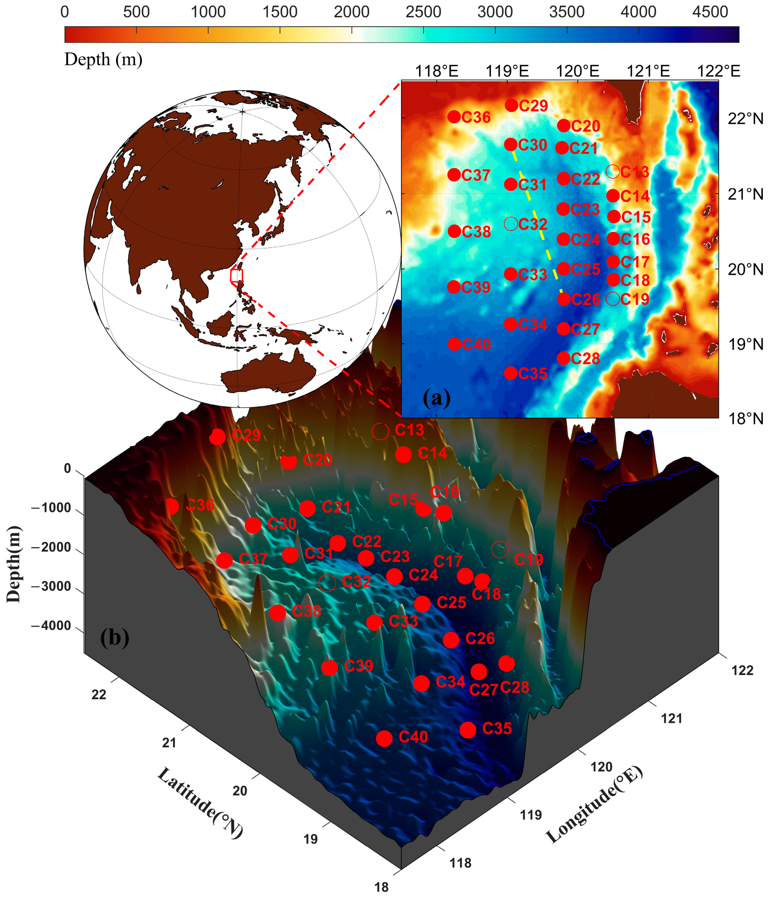
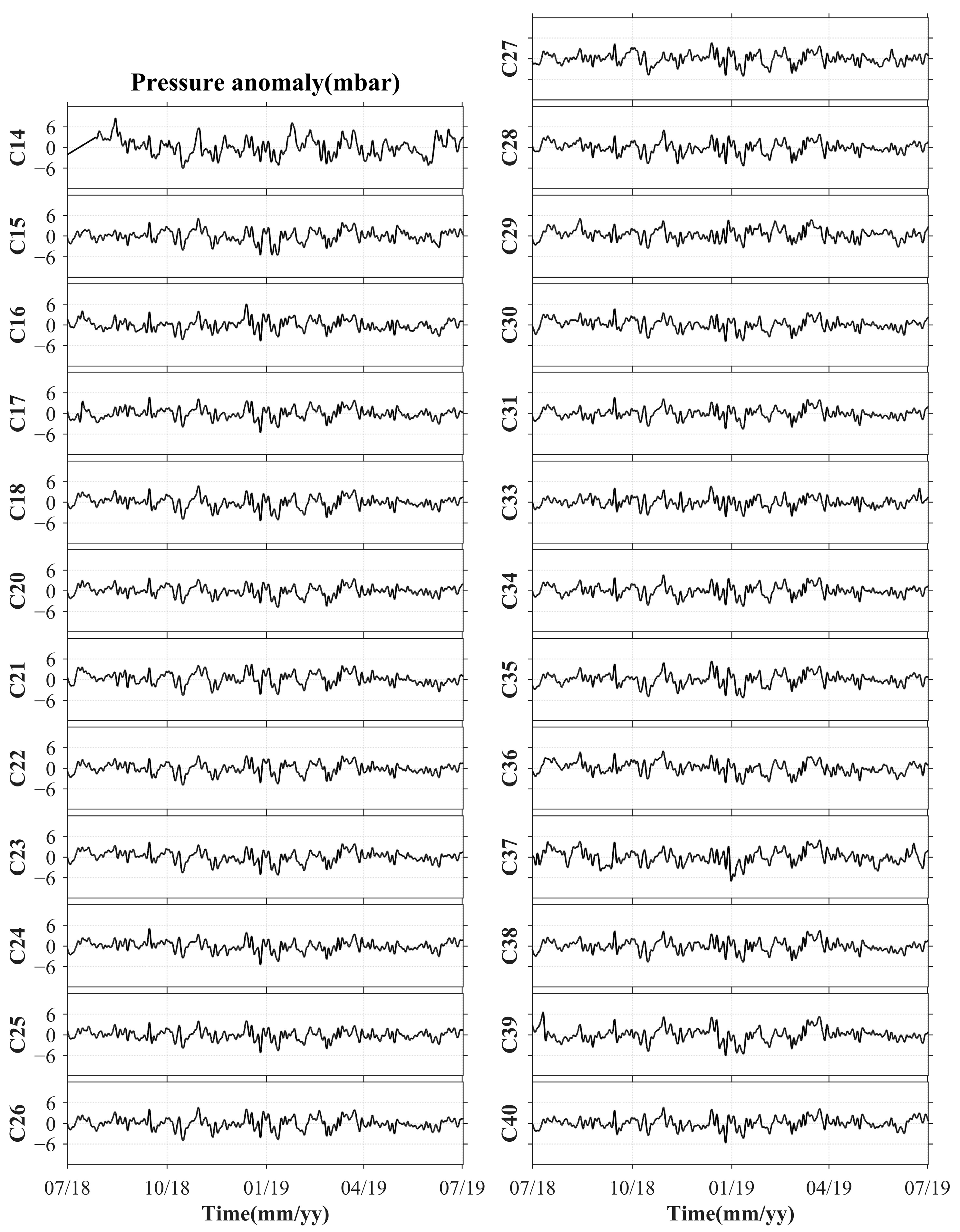
2.1. PIES OBP Measurements

To characterize the temporal and spatial evolution of the three-dimensional oceanographic features in the northeastern SCS, 28 PIESs were deployed west of the LS and operated for over 400 days, starting from June 2018 and concluding in July 2019 (Figure 1) [38,39,40]. This array covered an area of approximately 100,000 km² from 18.5° to 22.5°N and 118° to 120.5°E. Long-term and high-precision OBP observations were collected at each site during the campaign.

The PIES is an advanced device for measuring the round-trip acoustic travel time and OBP; it consists of an Inverted Echo Sounder (IES) anchored to the seabed and is equipped with a high-resolution pressure gauge. OBP records were measured by Digiquartz 410 K series pressure sensors that were developed by Paroscientific Inc. (Redmond, DC, USA) with a sampling interval of 10 min, an absolute accuracy of ±0.01%, and a resolution of 0.1 mbar (1 mbar = 100 Pa) (IES User Manual, http://www.po.gso.uri.edu/dynamics/IES/index.html (accessed on 20 May 2022)).

Most of the PIES recorded OBP during the entire observation period, with the exception of C13, C19, and C32. Specifically, C13 may have moved, C19 was not successfully recovered, and C32 had some missing data. Therefore, the OBP data from 25 stations were used in this study. By employing the procedures proposed by Kennelly et al. (2007), the raw OBP records were despiked, detided, and dedrifted [41]. All OBP records were resampled at 1 h intervals and low-pass filtered for 72 h with a fourth-order Butterworth filter. Finally, the recorded time tags were converted to Universal Time Coordinated (UTC). The processed time series of the OBP anomalies are shown in Figure 2. The OBP anomaly records provided by PIES almost entirely cover the area west of LS. These records indicate that the spatial variability of OBP in the northeastern SCS is limited. Specifically, the maximum standard deviation of the spatial differences was only 0.54 mbar (Figure 3), with the largest OBP anomaly amplitude observed at C14 reaching approximately 8 mbar, and the remaining stations showing amplitudes around 6 mbar. Notably, the maximum standard deviation was much smaller than these observed amplitudes, which suggests that there were no significant spatial differences in the OBP variations in the northeastern SCS.

2.2. GRACE-FO Mascon Solutions

The GRACE-FO mascon solutions provided by the Jet Propulsion Laboratory (JPL) (https://podaac.jpl.nasa.gov/dataset/TELLUS_GRAC-GRFO_MASCON_CRI_GRID_RL06_V2 (accessed on 14 July 2022)), Center for Space Research (CSR) (https://www2.csr.utexas.edu/grace/RL06_mascons.html (accessed on 14 July 2022)), and Goddard Space Flight Center (GSFC) (https://earth.gsfc.nasa.gov/geo/data/grace-mascons (accessed on 19 July 2022)) were used in this study. The data are presented in an equivalent water height with a temporal resolution of one month [42,43,44]. Detailed information on the mascon solutions from the three institutions is presented in

Table 1. The overview of the GRACE-FO mascon solutions.

Institution	JPL	CSR	GSFC
Version	RL06 2.0	RL06 2.0	RL06 1.0
Original Resolution	3° × 3°	1° × 1°	1° × 1°
Grid size	0.5° × 0.5°	0.25° × 0.25°	0.5° × 0.5°

.

2.3. Validation of GRACE-FO’s Accuracy

GRACE-FO OBP anomalies at each PIES station were obtained using spatial interpolation. As the GRACE/GRACE-FO mascon solutions are provided with monthly sampling, the OBP records from the PIESs were averaged monthly before comparison.

Initially, station-averaged OBP anomalies from PIES and GRACE-FO were compared. The accuracy of the GRACE-FO mascon solutions to represent the OBP variations in the SCS was evaluated by calculating the root mean square difference (RMSD) and correlation between PIES and GRACE-FO. To reduce the potential impact of the spatial average on the comparison, and to identify the differences between the various sites, in situ comparisons were conducted at each station, and the correlation and RMSD of PIES and GRACE-FO were calculated.

2.4. Calculation of Abyssal Volume Transport

OBP anomalies have been used to estimate variations in abyssal ocean volume transport in large-scale ocean currents [45,46,47,48]. Bingham and Hughes (2008) proposed a method to calculate northward transport along a particular depth in the North Atlantic based on the OBP difference between the east and west boundaries [45]. Landerer et al. (2015) utilized this approach and GRACE records to determine the variability of the North Atlantic meridional overturning transport between 3000 and 5000 m [46]. Similarly, based on OBP data from the ECCO, Zhu et al. (2022) quantified long-term variations in the LS overflow transport, which showed a downward trend in its strength during the last 20 years [47]. Moreover, comparable methods have demonstrated a weakening trend in the abyssal circulation of the SCS over the past decade [48]. Based on these studies, the volume transport variations of abyssal circulation via a particular section in the SCS can be estimated based on the OBP difference between the two ends of the section. Assuming that barotropic circulation exists in the abyssal SCS and that geostrophy governs the large-scale flow, the transport processes can be expressed as an integral of the momentum equation [45]:

$${\int }_{y_2}^{y_1}fVdy=\frac{1}{\rho }{\int }_{y_2}^{y_1}-\frac{\partial P}{\partial y}dy,$$

(1)

this integral is taken from one end of the section $y_2\left(y,h\right)$ to the other end $y_1\left(y,h\right)$, wherein the depth $h$ remains constant and y is a coordinate direction. Note here that the y-axis is defined as the axis along the direction of section C26–C30 (Figure 1) rather than the traditional meridian (South–North). On the left-hand side of the equation, the Coriolis force is integrated in the $y$ direction, whereas on the right-hand side, the pressure gradient force is integrated in the same direction. Note that the acceleration terms and friction effects were ignored. Where $V$ is the flow perpendicular to the section, $f$ and $\rho$ are the Coriolis parameter and the seawater density, respectively.

The horizontal integral of $V$ is expressed as $T$, which is the volume transported through a particular depth in a section. Thus Equation (1) can be abbreviated as

$$T=\frac{P_1-P_2}{\rho f},$$

(2)

where $P_1$ and $P_2$ are the OBP anomalies at the two ends of the section. Note that the transport $T$ in Equation (2) is defined as positive in the direction perpendicular to the cross-section and westward. Finally, the volume transport $Q$ that is perpendicular to the cross-section can be obtained by integrating from the lower boundary $H_L$ to the upper boundary $H_{\mathit{U}}$:

$$Q={\int }_{H_L}^{H_U}\left(\frac{P_1-P_2}{\rho f}\right)dh$$

(3)

Zheng et al. (2022) [40] characterized the structure of the abyssal circulation west of the LS based on PIES observations. Their findings suggest that abyssal circulation flows southwestward at the western boundary of the basin, and the abyssal volume transport can be estimated by the cross-sectional flow between C26 and C30 (indicated by the yellow dashed line in Figure 1). Here, we also calculated the volume transport anomaly between C26 and C30 with OBP records, and compared it with the volume transport variations along the western boundary found by Zheng et al. (2022) [40].

3. Results and Discussion

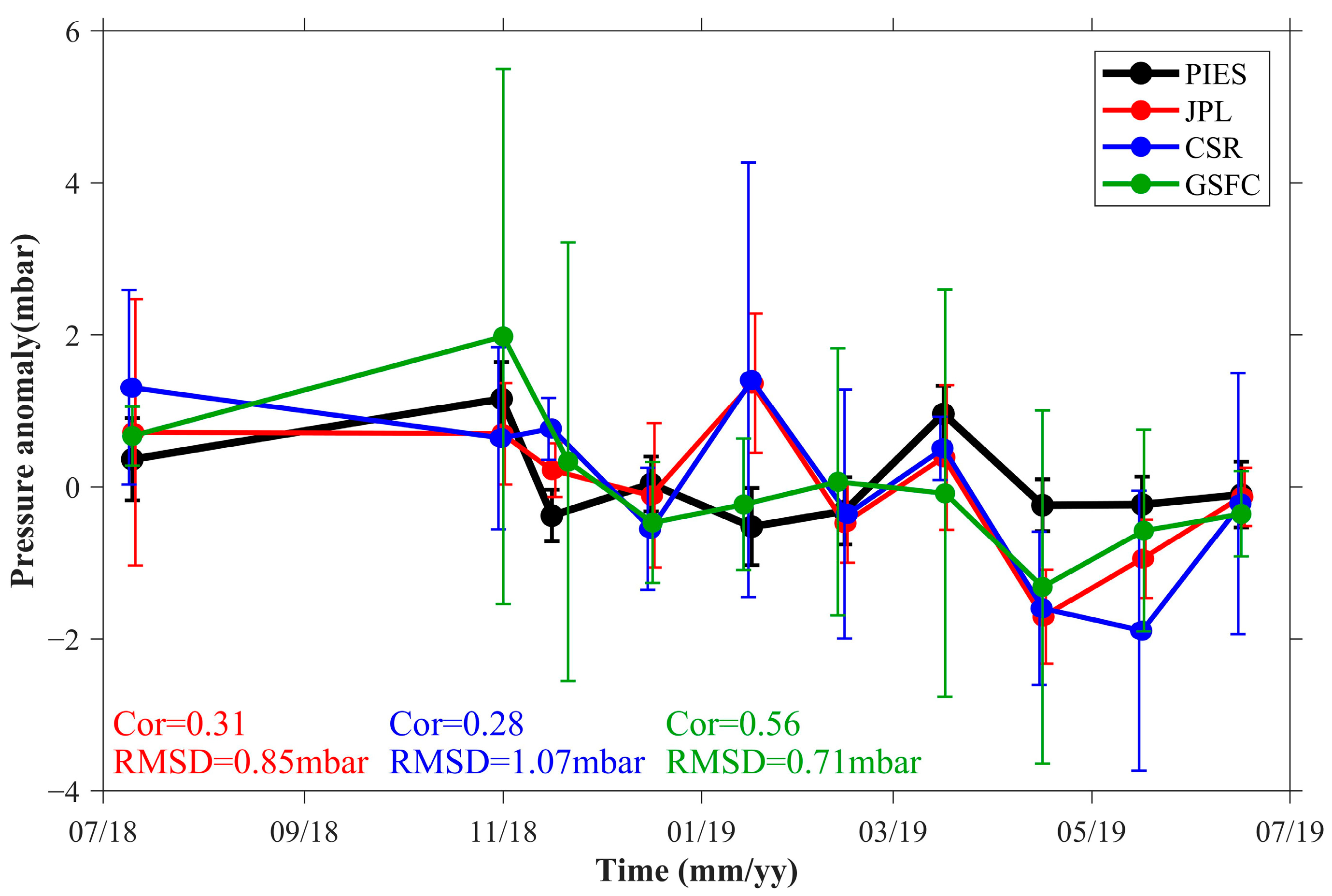
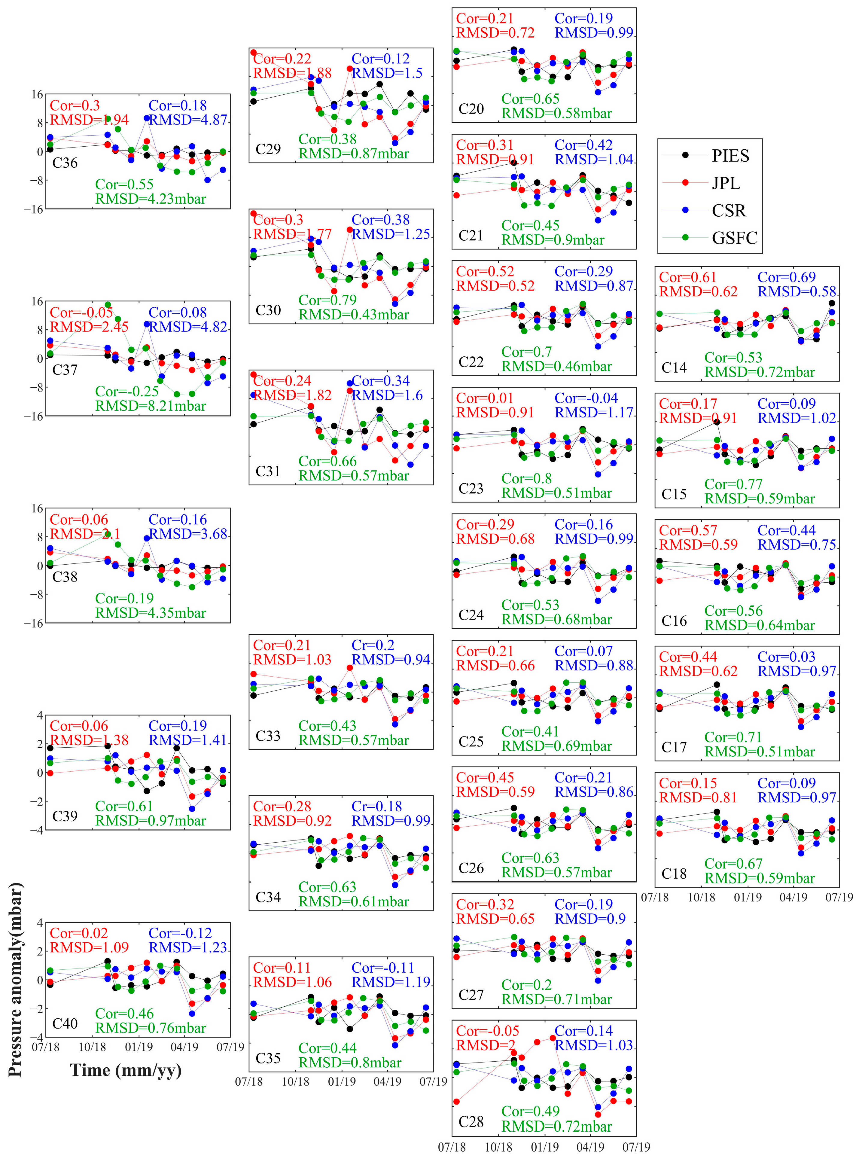
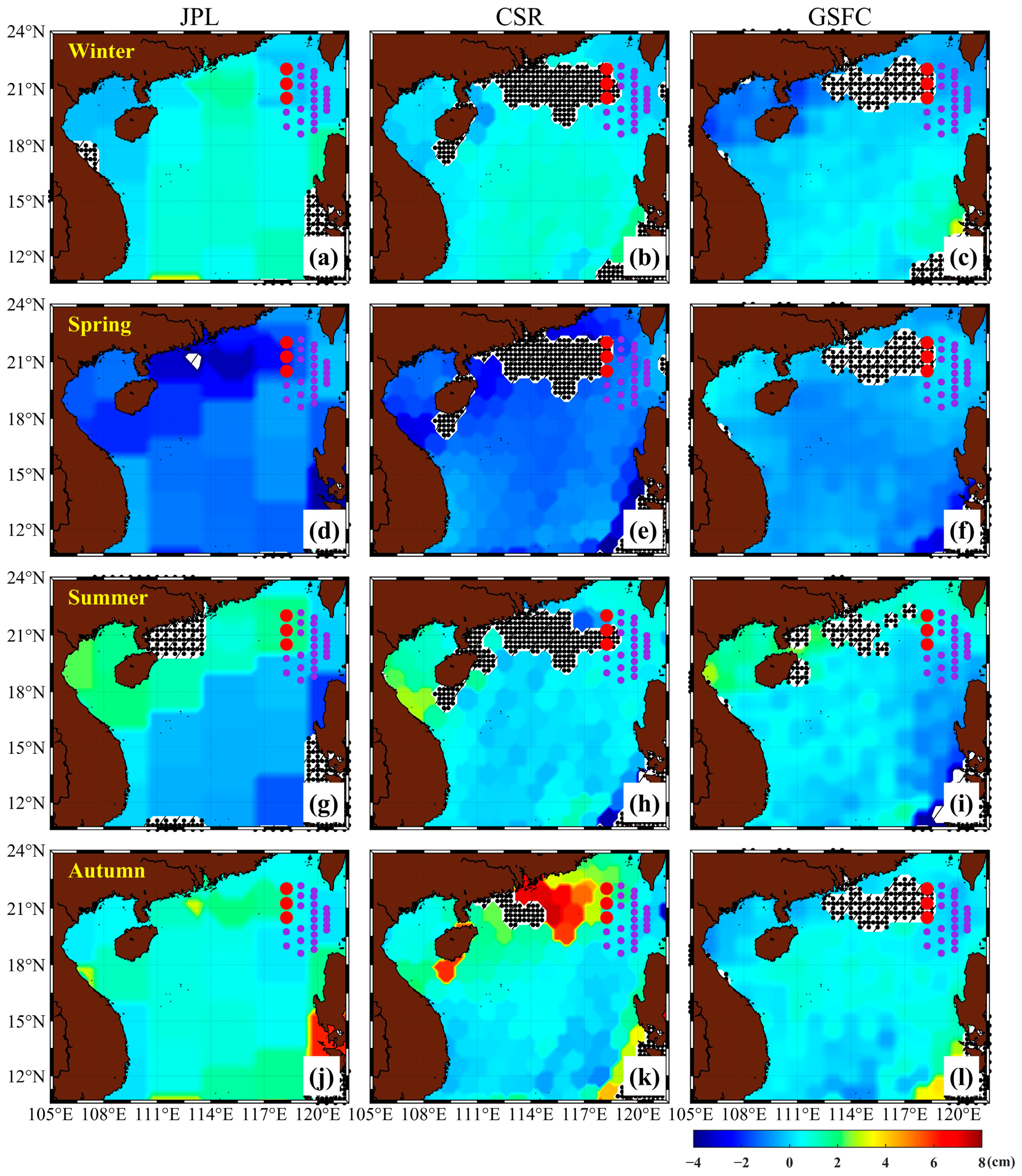
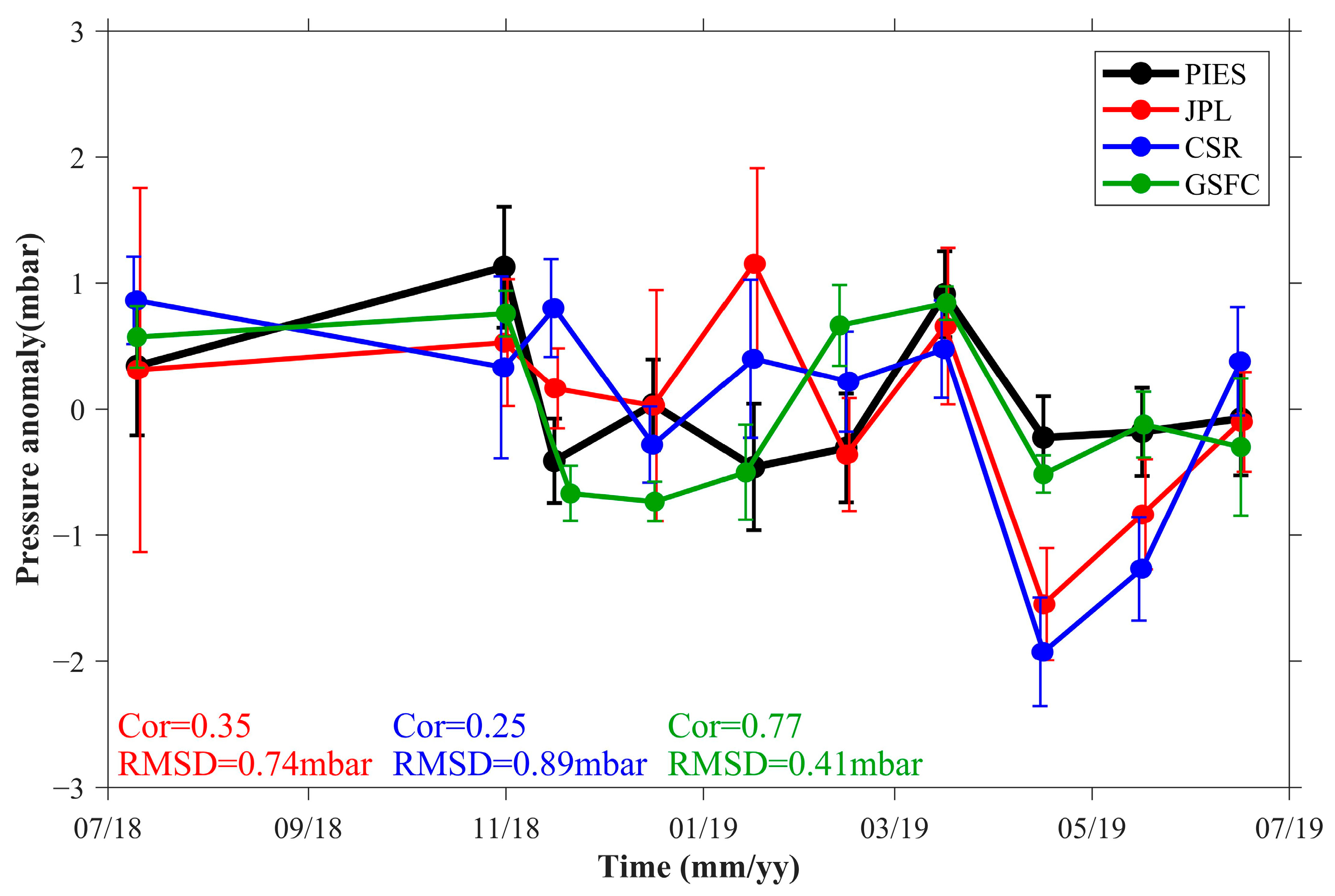
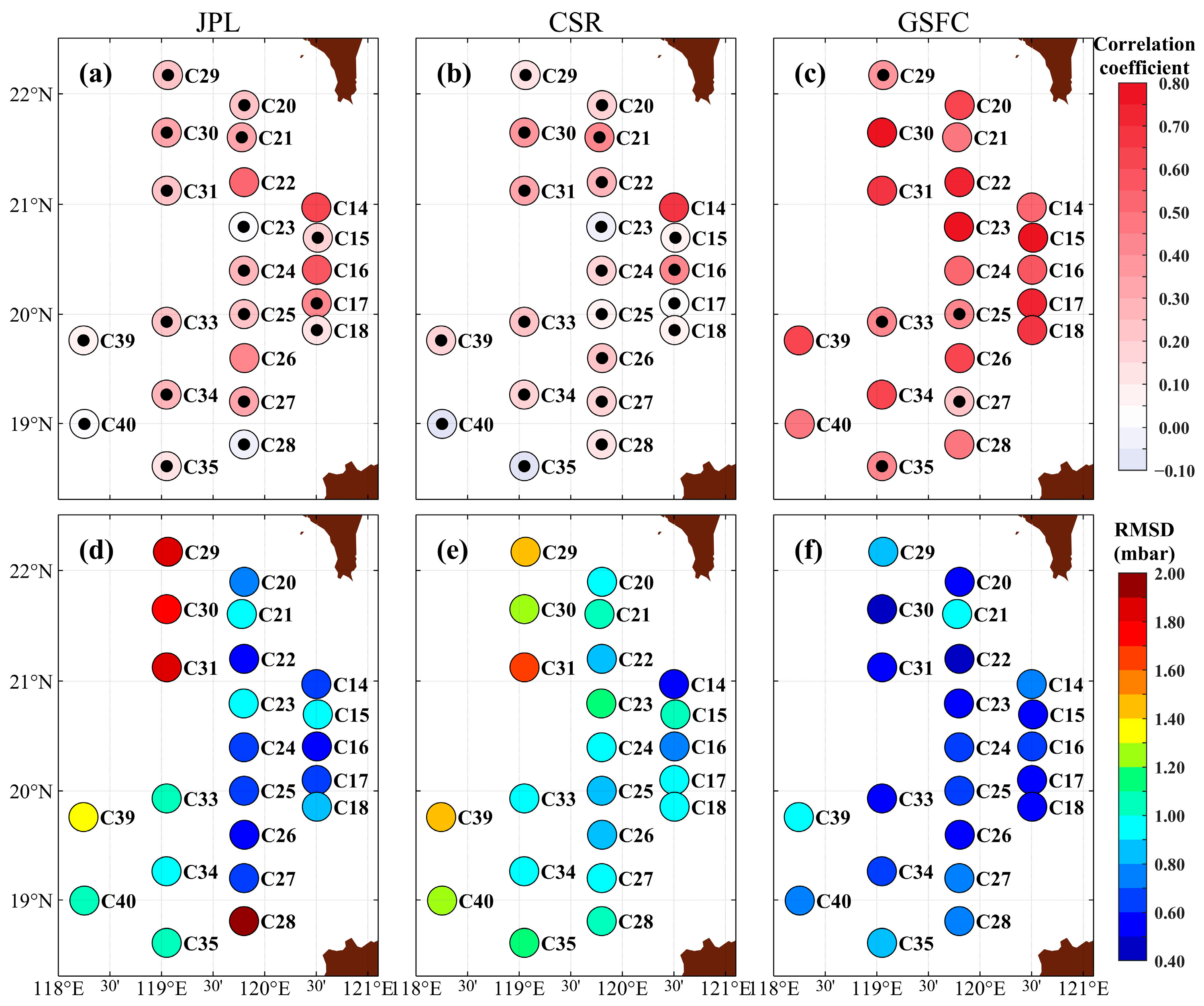
3.1. Comparison of OBP between GRACE-FO and PIES

The comparison between the station-averaged OBP anomalies from PIES and GRACE-FO is illustrated in Figure 3. The correlation coefficient (Cor) and RMSD between PIES and GSFC were 0.56 and 0.71 mbar, respectively. The correlation is statistically significant when the p-value = 0.04. The comparison between the mascon solutions provided by the other two institutes (JPL and CSR) and the PIES observations showed that their correlation with PIES observations was lower than that of GSFC, while their RMSD was higher. Specifically, the Cor was 0.31 (p-value = 0.19) and 0.28 (p-value = 0.22) for JPL and CSR, respectively, and the RMSD was 0.85 mbar and 1.07 mbar for JPL and CSR, respectively. As evident from the vertical bars in Figure 3, the spatial variability of the GRACE-FO mascon solutions was considerably more pronounced than that of the PIES observations.

The interpolated GRACE-FO OBP anomalies at each PIES station were then compared to the in situ OBP series (Figure 4). With the exception of C36—C38, the RMSD between GSFC and PIES was 0.4–1.0 mbar, and the Cor of most stations was above 0.4 (C27 and C29 were relatively small at 0.2 and 0.38, respectively). The RMSD between PIES and JPL (CSR) at all stations was 0.5–2.0 mbar (0.5–1.6 mbar) with the exception of C36—C38. The Cor between PIES and JPL (CSR) was less than 0.6 (0.5), with the exception of C14, which was approximately 0.2 (0.1). In addition, the Cor (RMSD) between the mascon solutions of the three institutions and the PIES OBP anomaly was significantly reduced (increased) at C36, C37, and C38. Despite the Cor between the GSFC and the PIES being 0.55 at C36, the RMSD was high at 4.23 mbar. The correspondence between PIES and JPL (CSR) at C36 was also poor, with a Cor of 0.3 (0.18) and a RMSD of 1.94 mbar (4.87 mbar). Additionally, GSFC had a low correlation with PIES at the C37 and C38, with a Cor of only −0.25 and 0.19 and a RMSD of 8.21 mbar and 4.35 mbar, respectively. JPL and CSR also showed a very low correlation with PIES observations and a relatively large RMSD at C37 and C38. Therefore, it can be seen that the mascon solutions from the three institutions had a poor agreement with the PIES records at C36, C37, and C38.

The variations in OBP from GRACE-FO could have been considerably overestimated on the continental shelf of the SCS, which resulted in significant discrepancies between the mascon solutions from the three institutions and the PIES measurements at C36, C37, and C38. Figure 5 shows maps of the winter, spring, summer, and autumn OBP changes that were deduced from the three GRACE-FO mascon solutions in the SCS during the PIES observation period (July 2018 to June 2019). Evidently, GRACE-FO overestimated the variations in the OBP near the SCS coast and northern slopes (stippled overlay areas in Figure 5). This could be because of signal leakage from the continents, although hydrological signals have been delimited (to some extent) from oceanic mass changes in the GRACE-FO mascon processing strategy [49]. At C36, C37, and C38, which are situated on the northern slopes of the SCS, the OBP anomalies obtained from GRACE-FO and PIES showed poor agreement.

Given their low quality, the GRACE-FO time series at stations C36, C37, and C38 are henceforth excluded. The station-averaged records from the other 22 sites are shown in Figure 6. It is evident from the bars (Figure 6) that the spatial variability of the GRACE-FO mascon solution decreased significantly when compared to that seen in Figure 3, and is comparable to the spatial variability observed in PIES stations, with the exception of JPL in July 2018. When C36, C37, and C38 were removed from the analysis, the consistency between the three GRACE-FO mascon solutions and the PIES measurements improved. The GRACE-FO OBP anomaly provided by the GSFC (green line) shows high consistency with the PIES station-averaged values (black line), with a Cor of 0.77 and an RMSD of 0.41 mbar. The correlation is statistically significant at a p-value = 0.005. In Figure 6, the maximum variation in GSFC is approximately 2.0 mbar. With an RMSD of 20% relative to the maximum variation, these results indicate that the GRACE-FO OBP anomaly provided by GSFC possesses sufficient accuracy to effectively capture the monthly variations in the OBP in the SCS. In contrast, the GRACE-FO mascon solutions provided by JPL (red line) and CSR (blue line) still exhibit some differences from the PIES measurements, with a Cor of only 0.35 (p-value = 0.16) and 0.25 (p-value = 0.24) and a RMSD of 0.74 mbar and 0.89 mbar, respectively. Additionally, the difference in correlation between GSFC and JPL (CSR) is 0.42 (0.52), which is deemed statistically significant at a p-value = 0.1 (0.08). Although the RMSDs of these GRACE-FO products are significantly smaller than the comparative results for the Kuroshio Extension region in Park et al. (2008) (1.4–1.7 mbar) [22], our evaluation suggests that the OBP variations in the SCS are more accurately represented by the GRACE-FO mascon solutions provided by the GSFC than those provided by JPL and CSR between July 2018 and June 2019.

Figure 7a–c present the Cor between the GRACE-FO mascon solutions and the in situ PIES measurements on a point-wise basis. Any doubtful data at C36, C37, and C38 were excluded from GRACE-FO prior to analysis. The GRACE-FO OBP anomaly (GSFC) showed a high correlation with the PIES OBP anomaly, with a Cor greater than 0.4 at most stations except for regions around C27—where the Cor was near 0.2. Meanwhile, the correlation of other stations, except for C25, C27, C29, C33, and C35, was statistically significant (p-value < 0.1). In contrast, the JPL and CSR OBP series had a lower correlation with the PIES OBP series, with a Cor mostly around 0.2 and 0.1, respectively (except near C14 and C16, where the Cor is greater than 0.5). Additionally, the correlation between the JPL OBP series and the PIES OBP series was statistically insignificant except for C14, C16, C22, and C26 (p-value > 0.1). As for the CSR OBP series, its correlation with the PIES OBP series was statistically significant only for C14 (p-value < 0.1). Figure 7d–f shows the corresponding point-wise RMSD between the three GRACE-FO mascon solutions and the PIES measurements. The RMSD between GSFC and PIES is concentrated between 0.4–0.9 mbar at most stations, whereas JPL (CSR) is between 0.5–2.0 mbar (0.5–1.6 mbar). These values indicate that the GRACE-FO mascon solutions (GSFC) better represent the OBP variations in the SCS, which is consistent with the overall average results for the stations. However, this does not mean that the GSFC has better accuracy in all ocean regions as Mu et al. (2019) [50] proved: the accuracy of the GRACE-FO mascon solutions provided by different institutions varies widely across different regions. This inference underscores the need for more in situ measurements to assess the uncertainties of GRACE-FO satellite products in representing long-term OBP variations.

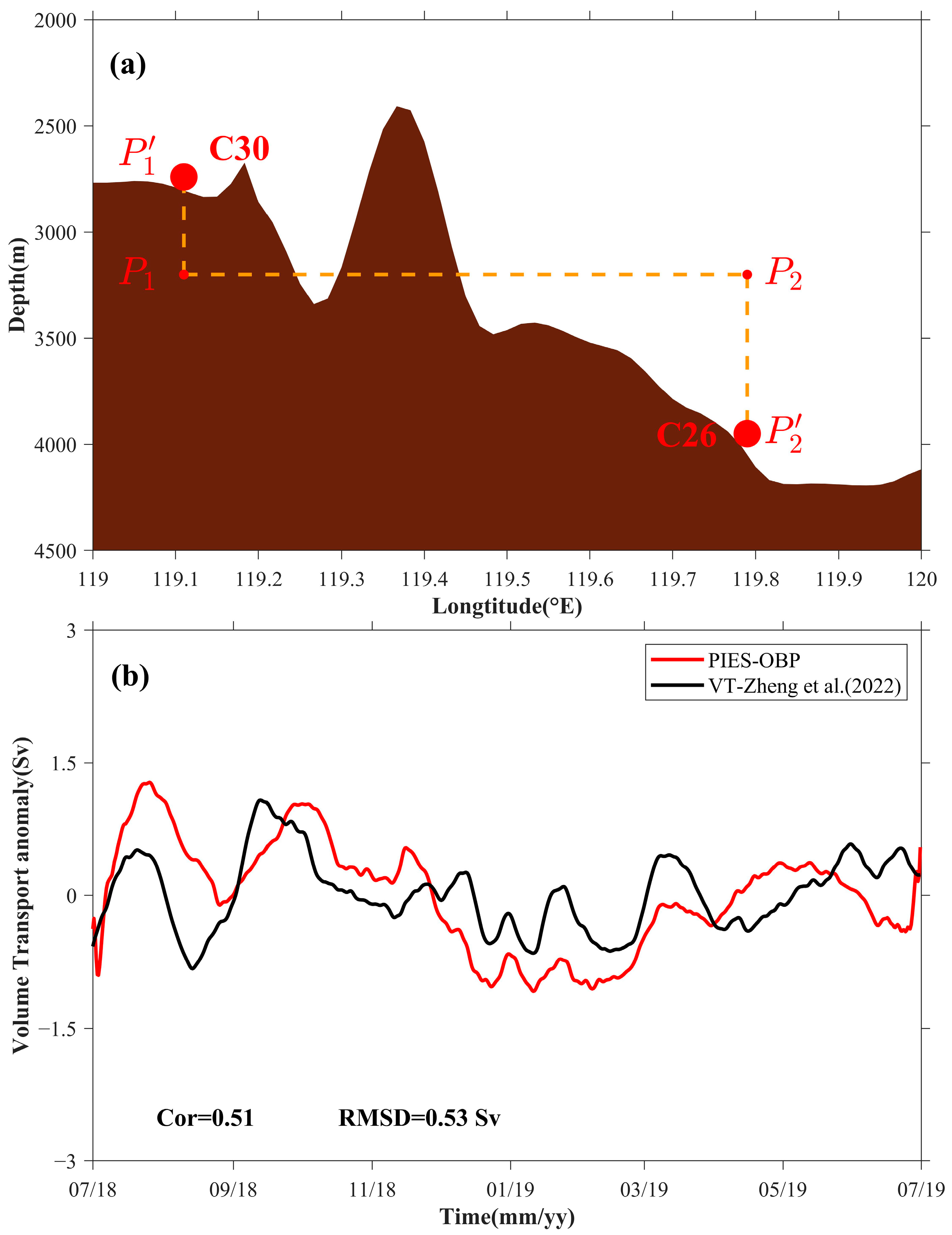
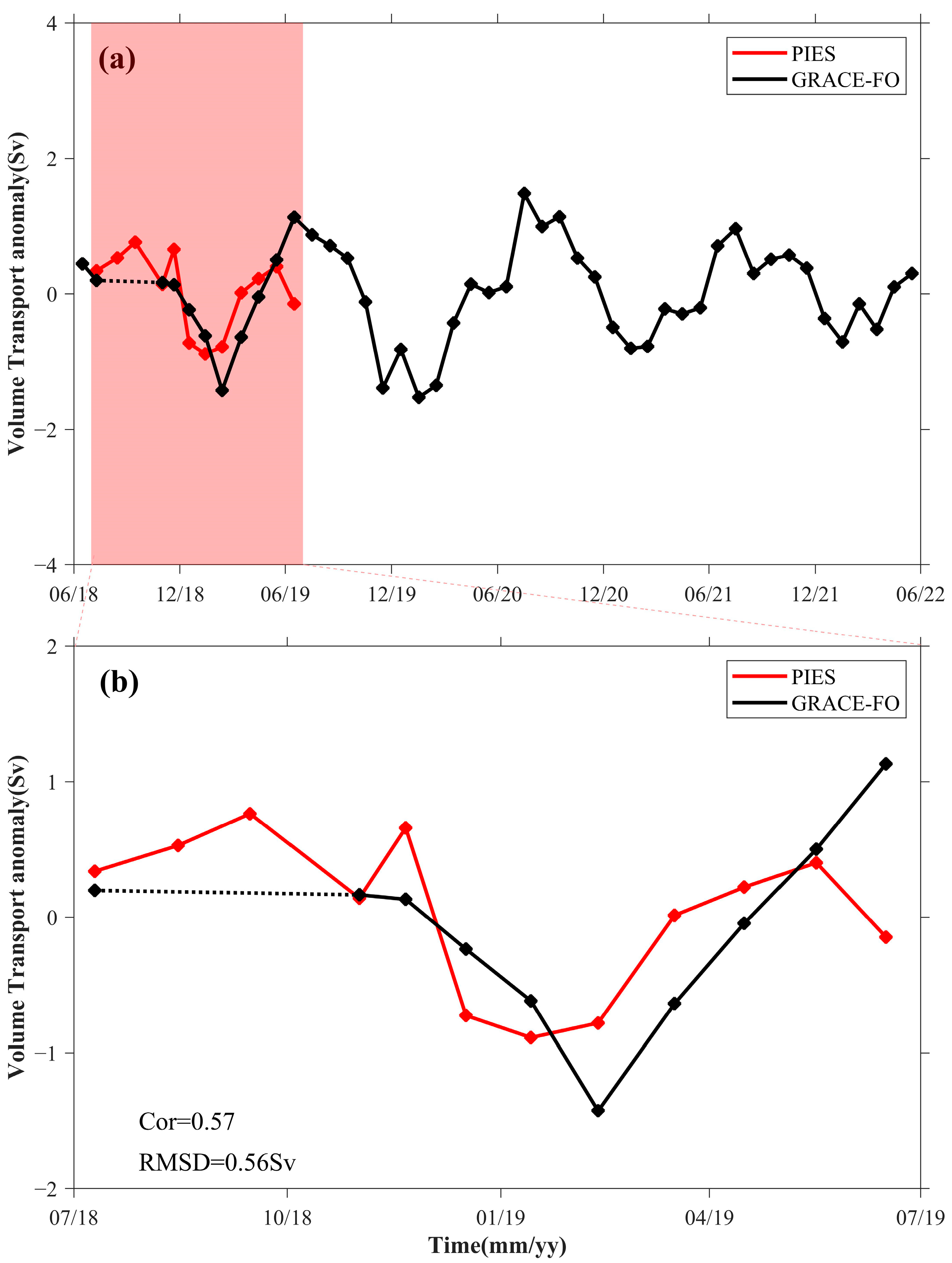
3.2. Application to Transport Monitoring

Variations in the SCS abyssal volume transport were calculated using GRACE-FO (GSFC) mascon solutions and PIES records at C26 and C30, and the feasibility of employing GRACE-FO (GSFC) for this purpose in the SCS was evaluated by adequate comparisons to field measurements of transport. Prior to this comparison, it was necessary to verify that the point-wise OBP anomalies allow for monitoring variations in the SCS abyssal volume transport.

A cross-section of the topography between stations C26 and C30 is presented in Figure 8a with depths of 3940 and 2600 m at C26 and C30, respectively. In the calculation, the bottom boundary of the abyssal circulation in the SCS was assumed to be the average depth of these two stations—that is, $H_L$ in Equation (3) was considered to be 3200 m. The upper boundary $H_U$ was set at 2500 m [40]. As the depths of C26 and C30 are different, it was assumed that the OBP anomaly has minimal depth-dependent variation in the deep layers—that is, $P_1$ = $P_1^{\prime }$ and $P_2$ = $P_2^{\prime }$ [51]. Here, $P_1^{\prime }$ and $P_2^{\prime }$ are the measured OBP anomalies from the PIES at the C30 and C26, respectively, and $P_1$ and $P_2$ represent the corresponding OBP anomalies at a depth of 3200 m.

The volume transport anomaly across C26–C30 (red line in Figure 8b) was calculated from the difference between $P_1$ and $P_2$. The Cor between our calculation and the variations in the deep-layer volume transport of the western boundary current are presented in Figure 14a (from Zheng et al. (2022) [40]). The black line in Figure 8b is 0.51, with an RMSD of 0.53 Sv (1 Sv = 10⁶ m³/s). Although there are some differences between these two estimates, the general agreement is encouraging and underpins the feasibility to monitor the abyssal volume transport anomaly by using the differences in the OBP anomalies. In other words, it is suggested that Equation (3) can be used to calculate the abyssal volume transport variations in SCS as the observed differences may be attributed to the topography effect between $P_1$ (C30) and $P_2$ (C26) (cf. Bingham and Hughes (2008) for a discussion [45].)

Following this verification, we then used the GSFC OBP anomalies to calculate the abyssal volume transport variations in the SCS over a period of four years, from June 2018 to June 2022. These transports, represented by the black line in Figure 9a, show a pronounced seasonal signal, with a sharp decrease in volume transport in late winter and early spring, and a peak in late summer and early autumn, which is closely aligned with the findings of Zheng et al. (2022) [40]. In addition, the seasonal cycle in the SCS abyssal volume transport obtained in this study is similar to the seasonal variations in the LS overflow transport calculated by Zhu et al. (2022) [47] (both studies used the ECCO OBP anomaly with the same method). Comparing our monthly abyssal transport estimates with the monthly averaged transport series from the PIES (red line in Figure 9), we find Cor = 0.57 and RMSD = 0.56 Sv. The correlation is statistically significant at the p-value = 0.04. According to the GRACE-FO computation, the monthly sampled SCS abyssal volume transport changes exhibited a peak of approximately 3.2 Sv in summer 2020 (Figure 9a). Given that the RMSD relative to the PIES transport estimates is much smaller than this and other maxima, we conclude that GRACE-FO has sufficient accuracy to effectively capture the monthly variations in SCS abyssal volume transport; in addition, the GRACE-FO mascon solutions provided by the GSFC can be used for the long-term monitoring of seasonal or longer-period variations in SCS abyssal volume transport.

4. Conclusions

This study utilized the long-term, high-precision, and high-resolution OBP measurements provided by the PIES array west of the LS to validate the accuracy and applicability of the GRACE-FO mascon solutions from the JPL, the CSR, and the GSFC over a period of 10 months from July 2018 to June 2019 (with satellite data missing for August and September 2018). In the northeastern SCS, both station-averaged and in situ comparisons showed that the mascon solutions provided by the GSFC outperformed those of the CSR and JPL in characterizing the OBP variations between July 2018 and June 2019. Additionally, this study found that the OBP variations estimated by GRACE-FO near the coast of the SCS and the northern continental slope were much larger than those in other regions, possibly because of signal leakage.

This study further evaluated the feasibility of applying GRACE-FO (GSFC) mascon solutions to the SCS by calculating the volume transport anomaly in the deep SCS. These satellite-based volume transports were found to be consistent with the results that were calculated via the PIES OBP anomaly. The SCS abyssal volume transport sharply decreased in late winter and early spring, peaked in midsummer and early autumn, and exhibited a seasonal cycle that is very similar to those documented in previous studies. This indicates that the GRACE-FO mascon solutions provided by the GSFC can be effectively applied to the study of seasonal or longer-period variations in the abyssal circulation in the SCS. Note that although the grid size of GRACE-FO mascon from GSFC is 0.5° × 0.5°, the cross-section used to calculate variations in SCS abyssal volume transport must be long enough to satisfy the spatial resolution limitations of GSFC. Moreover, the cross-section should be as far away from land or regions with as steep terrain as possible to mitigate the impact of signal leakage.

Currently, our understanding of the response of the SCS abyssal circulation to long-term trends in ocean mass variations is still limited. The validation and evaluation of the accuracy of the GRACE-FO estimates in the SCS are expected to provide a reliable foundation for the application of long-term, spatially continuous OBP data from GRACE-FO in the SCS. At the same time, this study also serves as a valuable reference for the application of GRACE-FO mass change products in other regions.

References

1. Tapley, B.D.; Bettadpur, S.; Watkins, M.; Reigber, C. The gravity recovery and climate experiment: Mission overview and early results. Geophys. Res. Lett. 2004, 31, L09607. [Google Scholar] [CrossRef]
2. Landerer, F.W.; Flechtner, F.M.; Save, H.; Webb, F.H.; Bandikova, T.; Bertiger, W.I.; Bettadpur, S.V.; Byun, S.H.; Dahle, C.; Dobslaw, H.; et al. Extending the Global Mass Change Data Record: GRACE Follow-On Instrument and Science Data Performance. Geophys. Res. Lett. 2020, 47, e2020GL088306. [Google Scholar] [CrossRef]
3. Shang, P.; Su, X.; Luo, Z. Characteristics of the Greenland Ice Sheet Mass Variations Revealed by GRACE/GRACE Follow-On Gravimetry. Remote Sens. 2022, 14, 4442. [Google Scholar] [CrossRef]
4. Velicogna, I.; Mohajerani, Y.; A, G.; Landerer, F.; Mouginot, J.; Noel, B.; Rignot, E.; Sutterley, T.; van den Broeke, M.; van Wessem, M.; et al. Continuity of Ice Sheet Mass Loss in Greenland and Antarctica from the GRACE and GRACE Follow-On Missions. Geophys. Res. Lett. 2020, 47, e2020GL087291. [Google Scholar] [CrossRef]
5. Feng, W.; Zhong, M.; Lemoine, J.-M.; Biancale, R.; Hsu, H.-T.; Xia, J. Evaluation of groundwater depletion in North China using the Gravity Recovery and Climate Experiment (GRACE) data and ground-based measurements. Water Resour. Res. 2013, 49, 2110–2118. [Google Scholar] [CrossRef]
6. Xie, Y.; Huang, S.; Liu, S.; Leng, G.; Peng, J.; Huang, Q.; Li, P. GRACE-Based Terrestrial Water Storage in Northwest China: Changes and Causes. Remote Sens. 2018, 10, 1163. [Google Scholar] [CrossRef]
7. Willis, J.K.; Chambers, D.P.; Nerem, R.S. Assessing the globally averaged sea level budget on seasonal to interannual timescales. J. Geophys. Res. 2008, 113, C06015. [Google Scholar] [CrossRef]
8. Chambers, D.P.; Cazenave, A.; Champollion, N.; Dieng, H.; Llovel, W.; Forsberg, R.; von Schuckmann, K.; Wada, Y. Evaluation of the Global Mean Sea Level Budget between 1993 and 2014. Surv. Geophys. 2016, 38, 309–327. [Google Scholar] [CrossRef]
9. Poropat, L.; Dobslaw, H.; Zhang, L.; Macrander, A.; Boebel, O.; Thomas, M. Time Variations in Ocean Bottom Pressure from a Few Hours to Many Years: In Situ Data, Numerical Models, and GRACE Satellite Gravimetry. J. Geophys. Res. Ocean. 2018, 123, 5612–5623. [Google Scholar] [CrossRef]
10. Zheng, H.; Zhu, X.-H.; Nakamura, H.; Park, J.-H.; Jeon, C.; Zhao, R.; Nishina, A.; Zhang, C.; Na, H.; Zhu, Z.-N.; et al. Generation and propagation of 21-day bottom pressure variability driven by wind stress curl in the East China Sea. Acta Oceanol. Sin. 2020, 39, 91–106. [Google Scholar] [CrossRef]
11. Kanzow, T. Seasonal variation of ocean bottom pressure derived from Gravity Recovery and Climate Experiment (GRACE): Local validation and global patterns. J. Geophys. Res. 2005, 110, C09001. [Google Scholar] [CrossRef]
12. Wahr, J.; Molenaar, M.; Bryan, F. Time variability of the Earth’s gravity field: Hydrological and oceanic effects and their possible detection using GRACE. J. Geophys. Res. Solid Earth 1998, 103, 30205–30229. [Google Scholar] [CrossRef]
13. Wahr, J.M.; Jayne, S.R.; Bryan, F.O. A method of inferring changes in deep ocean currents from satellite measurements of time-variable gravity. J. Geophys. Res. Ocean. 2002, 107, 3218. [Google Scholar] [CrossRef]
14. Ponte, R.M.; Quinn, K.J.; Wunsch, C.; Heimbach, P. A comparison of model and GRACE estimates of the large-scale seasonal cycle in ocean bottom pressure. Geophys. Res. Lett. 2007, 34, L09603. [Google Scholar] [CrossRef]
15. Morison, J.; Wahr, J.; Kwok, R.; Peralta-Ferriz, C. Recent trends in Arctic Ocean mass distribution revealed by GRACE. Geophys. Res. Lett. 2007, 34, L07602. [Google Scholar] [CrossRef]
16. Chambers, D.P.; Willis, J.K. A Global Evaluation of Ocean Bottom Pressure from GRACE, OMCT, and Steric-Corrected Altimetry. J. Atmos. Ocean. Technol. 2010, 27, 1395–1402. [Google Scholar] [CrossRef]
17. Peralta-Ferriz, C.; Morison, J.H.; Wallace, J.M.; Bonin, J.A.; Zhang, J. Arctic Ocean circulation patterns revealed by GRACE. J. Clim. 2014, 27, 1445–1468. [Google Scholar] [CrossRef]
18. Rietbroek, R.; LeGrand, P.; Wouters, B.; Lemoine, J.M.; Ramillien, G.; Hughes, C. Comparison of in situ bottom pressure data with GRACE gravimetry in the Crozet-Kerguelen region. Geophys. Res. Lett. 2006, 33, L21601. [Google Scholar] [CrossRef]
19. Ponte, R.M.; Quinn, K.J. Bottom pressure changes around Antarctica and wind-driven meridional flows. Geophys. Res. Lett. 2009, 36, L13604. [Google Scholar] [CrossRef]
20. Volkov, D.L.; Landerer, F.W. Nonseasonal fluctuations of the Arctic Ocean mass observed by the GRACE satellites. J. Geophys. Res. Ocean. 2013, 118, 6451–6460. [Google Scholar] [CrossRef]
21. Munekane, H. Ocean mass variations from GRACE and tsunami gauges. J. Geophys. Res. 2007, 112, B07403. [Google Scholar] [CrossRef]
22. Park, J.-H.; Watts, D.R.; Donohue, K.A.; Jayne, S.R. A comparison of in situ bottom pressure array measurements with GRACE estimates in the Kuroshio Extension. Geophys. Res. Lett. 2008, 35, L17601. [Google Scholar] [CrossRef]
23. Boening, C.; Lee, T.; Zlotnicki, V. A record-high ocean bottom pressure in the South Pacific observed by GRACE. Geophys. Res. Lett. 2011, 38, L04602. [Google Scholar] [CrossRef]
24. Johnson, G.C.; Chambers, D.P. Ocean bottom pressure seasonal cycles and decadal trends from GRACE Release-05: Ocean circulation implications. J. Geophys. Res. Ocean. 2013, 118, 4228–4240. [Google Scholar] [CrossRef]
25. Cheng, X.; Ou, N.; Chen, J.; Huang, R.X. On the seasonal variations of ocean bottom pressure in the world oceans. Geosci. Lett. 2021, 8, 29. [Google Scholar] [CrossRef]
26. Quinn, K.J.; Ponte, R.M. Estimating high frequency ocean bottom pressure variability. Geophys. Res. Lett. 2011, 38, L08611. [Google Scholar] [CrossRef]
27. Köhl, A.; Siegismund, F.; Stammer, D. Impact of assimilating bottom pressure anomalies from GRACE on ocean circulation estimates. J. Geophys. Res. Ocean. 2012, 117, C04032. [Google Scholar] [CrossRef]
28. Makowski, J.K.; Chambers, D.P.; Bonin, J.A. Using ocean bottom pressure from the gravity recovery and climate experiment (GRACE) to estimate transport variability in the southern Indian Ocean. J. Geophys. Res. Ocean. 2015, 120, 4245–4259. [Google Scholar] [CrossRef]
29. Peralta-Ferriz, C.; Woodgate, R.A. The Dominant Role of the East Siberian Sea in Driving the Oceanic Flow through the Bering Strait—Conclusions from GRACE Ocean Mass Satellite Data and In Situ Mooring Observations between 2002 and 2016. Geophys. Res. Lett. 2017, 44, 11,472–11,481. [Google Scholar] [CrossRef]
30. Koelling, J.; Send, U.; Lankhorst, M. Decadal Strengthening of Interior Flow of North Atlantic Deep Water Observed by GRACE Satellites. J. Geophys. Res. Ocean. 2020, 125, e2020JC016217. [Google Scholar] [CrossRef]
31. Zhao, R.; Zhu, X.-H.; Park, J.-H. Near 5-Day Nonisostatic Response to Atmospheric Surface Pressure and Coastal-Trapped Waves Observed in the Northern South China Sea. J. Phys. Oceanogr. 2017, 47, 2291–2303. [Google Scholar] [CrossRef]
32. Zhang, K.; Zhu, X.-H.; Zhao, R. Near 7-day response of ocean bottom pressure to atmospheric surface pressure and winds in the northern South China Sea. Deep Sea Res. Part I Oceanogr. Res. Pap. 2018, 132, 6–15. [Google Scholar] [CrossRef]
33. Yuan, D. A numerical study of the South China Sea deep circulation and its relation to the Luzon Strait transport. Acta Oceanol. Sin. 2002, 2, 187–202. [Google Scholar]
34. Gan, J.; Liu, Z.; Hui, C.R. A three-layer alternating spinning circulation in the South China Sea. J. Phys. Oceanogr. 2016, 46, 2309–2315. [Google Scholar] [CrossRef]
35. Cai, Z.; Gan, J.; Liu, Z.; Hui, C.R.; Li, J. Progress on the formation dynamics of the layered circulation in the South China Sea. Prog. Oceanogr. 2020, 181, 102246. [Google Scholar] [CrossRef]
36. Zhu, Y.; Sun, J.; Wang, Y.; Li, S.; Xu, T.; Wei, Z.; Qu, T. Overview of the multi-layer circulation in the South China Sea. Prog. Oceanogr. 2019, 175, 171–182. [Google Scholar] [CrossRef]
37. Wang, D.; Wang, Q.; Cai, S.; Shang, X.; Peng, S.; Shu, Y.; Xiao, J.; Xie, X.; Zhang, Z.; Liu, Z. Advances in research of the mid-deep South China Sea circulation. Sci. China Earth Sci. 2019, 62, 1992–2004. [Google Scholar] [CrossRef]
38. Zhao, R.; Zhu, X.-H.; Zhang, C.; Zheng, H.; Zhu, Z.-N.; Ren, Q.; Liu, Y.; Nan, F.; Yu, F. Summer anticyclonic eddies carrying Kuroshio waters observed by a large CPIES array west of the Luzon Strait. J. Phys. Oceanogr. 2023, 53, 341–359. [Google Scholar] [CrossRef]
39. Zheng, H.; Zhu, X.-H.; Chen, J.; Wang, M.; Zhao, R.; Zhang, C.; Zhu, Z.-N.; Ren, Q.; Liu, Y.; Nan, F. Observation of bottom-trapped topographic Rossby waves to the west of the Luzon Strait, South China Sea. J. Phys. Oceanogr. 2022, 52, 2853–2872. [Google Scholar] [CrossRef]
40. Zheng, H.; Zhu, X.-H.; Zhang, C.; Zhao, R.; Zhu, Z.-N.; Ren, Q.; Liu, Y.; Nan, F.; Yu, F. Observation of Abyssal Circulation to the West of the Luzon Strait, South China Sea. J. Phys. Oceanogr. 2022, 52, 2091–2109. [Google Scholar] [CrossRef]
41. Kennelly, M.; Tracey, K.; Watts, D.R. Inverted Echo Sounder Data Processing Manual; Graduate School of Oceanography, University of Rhode Island: Narragansett, RI, USA, 2007. [Google Scholar]
42. Watkins, M.M.; Wiese, D.N.; Yuan, D.-N.; Boening, C.; Landerer, F.W. Improved methods for observing Earth’s time variable mass distribution with GRACE using spherical cap mascons. J. Geophys. Res. Solid Earth 2015, 120, 2648–2671. [Google Scholar] [CrossRef]
43. Save, H.; Bettadpur, S.; Tapley, B.D. High-resolution CSR GRACE RL05 mascons. J. Geophys. Res. Solid Earth 2016, 121, 7547–7569. [Google Scholar] [CrossRef]
44. Loomis, B.D.; Luthcke, S.B.; Sabaka, T.J. Regularization and error characterization of GRACE mascons. J. Geod. 2019, 93, 1381–1398. [Google Scholar] [CrossRef]
45. Bingham, R.J.; Hughes, C.W. Determining North Atlantic meridional transport variability from pressure on the western boundary: A model investigation. J. Geophys. Res. 2008, 113, C09008. [Google Scholar] [CrossRef]
46. Landerer, F.W.; Wiese, D.N.; Bentel, K.; Boening, C.; Watkins, M.M. North Atlantic meridional overturning circulation variations from GRACE ocean bottom pressure anomalies. Geophys. Res. Lett. 2015, 42, 8114–8121. [Google Scholar] [CrossRef]
47. Zhu, Y.; Yao, J.; Xu, T.; Li, S.; Wang, Y.; Wei, Z. Weakening Trend of Luzon Strait Overflow Transport in the Past Two Decades. Geophys. Res. Lett. 2022, 49, e2021GL097395. [Google Scholar] [CrossRef]
48. Zhu, Y.; Yao, J.; Li, S.; Xu, T.; Huang, R.X.; Nie, X.; Pan, H.; Wang, Y.; Fang, Y.; Wei, Z. Decadal Weakening of Abyssal South China Sea Circulation. Geophys. Res. Lett. 2022, 49, e2022GL100582. [Google Scholar] [CrossRef]
49. Bentel, K.; Landerer, F.W.; Boening, C. Monitoring Atlantic overturning circulation and transport variability with GRACE-type ocean bottom pressure observations—A sensitivity study. Ocean. Sci. 2015, 11, 953–963. [Google Scholar] [CrossRef]
50. Mu, D.; Xu, T.; Xu, G. Detecting coastal ocean mass variations with GRACE mascons. Geophys. J. Int. 2019, 217, 2071–2080. [Google Scholar] [CrossRef]
51. Zhu, X.-H.; Zhao, R.; Guo, X.; Long, Y.; Ma, Y.-L.; Fan, X. A long-term volume transport time series estimated by combining in situ observation and satellite altimeter data in the northern South China Sea. J. Oceanogr. 2015, 71, 663–673. [Google Scholar] [CrossRef]
Figure 1. (a) Map of the study area in the South China Sea (SCS). The used (red dots) and not used (red circle) ocean bottom pressure (OBP) records at the pressure-recording inverted echo sounder (PIES) stations in the study are indicated. The yellow dashed line represents the section chosen for calculating the volume transport anomaly of abyssal circulation. (b) Topographic map of the seabed west of the Luzon Strait (LS) with the same spatial distribution as (a).
Remotesensing 15 02804 g001
Figure 2. The processed time series of the PIES OBP anomalies.
Remotesensing 15 02804 g002
Figure 3. Comparison between the station-averaged PIES OBP anomaly (C14–C18, C20–C31, and C33–C40) and the GRACE-FO OBP anomaly from July 2018 to June 2019. Note that the GRACE-FO data for August and September 2018 were missing because of sensor failure. The PIES OBP anomaly is represented by the black line, whereas the GRACE-FO OBP anomaly provided by JPL, CSR, and GSFC are represented by the red, blue, and green lines, respectively. The Cor and RMSD between PIES and GRACE-FO are displayed below the figure. The colors of the text correspond to the colors of the lines JPL (red), CSR (blue), and GSFC (green). Bars indicate the standard deviations of the spatial average.
Remotesensing 15 02804 g003
Figure 4. A comparison of the in situ GRACE-FO mascon solutions with PIES observations. The PIES data are represented by the black line, whereas the JPL, CSR, and GSFC estimates are represented by the red, blue, and green lines, respectively. Note that the y-axis ranges of the panels C36, C37, and C38 are −16 to 16, while the y-axis ranges of the remaining panels are −4 to 4. The Cor and RMSD between PIES and JPL (CSR) are shown above each panel, and the colors of the text correspond to the colors of the lines JPL (red) and CSR (blue), respectively. Statistics for GSFC (green) are shown below each panel.
Remotesensing 15 02804 g004
Figure 5. The seasonal pattern derived from the GRACE-FO mascon solutions in the SCS from July 2018 to June 2019 is represented at an equivalent water height. JPL (left), CSR (middle), and GSFC (right) are listed, and rows represent winter (ac), spring (df), summer (gi), and autumn (jl). Note that the winter in (ac) is the average of December 2018, January, and February 2019; spring in (df) is the average of March, April, and May 2019; summer in (gi) is the average of July 2018 and June 2019; and autumn in (jl) is the average of October and November 2018. Red dots represent C36, C37, and C38, whereas purple dots represent other stations. Note that only the GRACE-FO OBP anomaly within the seasonal mean plus or minus the standard deviation of that season were retained. The stippled overlay areas represent the regions in the ocean where the OBP variations were beyond the range of the seasonal mean plus or minus the standard deviation.
Remotesensing 15 02804 g005
Figure 6. Same as Figure 3, but with spatial averages computed without estimates at C36, C37, and C38.
Remotesensing 15 02804 g006
Figure 7. The Cor between the GRACE-FO OBP series from (a) JPL, (b) CSR, and (c) GSFC, as well as the PIES OBP anomalies. Background colors represent the magnitude of the Cor. A black dot on top of a circle indicates that the correlation at that station is statistically insignificant (p-value > 0.1), while a circle without a black dot indicates that the correlation at that station is statistically significant (p-value < 0.1). Panels (df) have the same form as (ac), but show the spatial distribution of RMSD.
Remotesensing 15 02804 g007
Figure 8. (a) Profile map of the seabed between C26 and C30 (yellow dashed line in Figure 1), with red dots indicating C26 and C30, and brown representing the seabed topography. (b) 30-day smoothed abyssal volume transport anomaly in the SCS. The red line represents the abyssal volume transport anomaly calculated using C30 and C26 observations projected onto points P 1  and P 2 at 3200 m depth, whereas the black line is modified from Figure 14a in Zheng et al. (2022) [40].
Remotesensing 15 02804 g008
Figure 9. (a) The calculated volume transport anomaly from June 2018 to June 2022 of the C26–C30 section, based on OBP anomalies from PIES (red line) and GSFC mascon solutions (black line). The black dotted line represents that the satellite data are missing here, including but not limited to August 2018 and September 2018. (b) The volume transport anomaly from July 2018 to June 2019, i.e., the shadowed part in (a). The Cor and RMSD are displayed in the lower left corner of the panel.
Remotesensing 15 02804 g009