Technical Note

Improving Crop Mapping by Using Bidirectional Reflectance Distribution Function (BRDF) Signatures with Google Earth Engine

by
Zhijun Zhen
1,2,†,
Shengbo Chen
1,3,†,
Tiangang Yin
4 and
Jean-Philippe Gastellu-Etchegorry
2,*
1
College of Geoexploration Science and Technology, Jilin University, Changchun 130026, China
2
CESBIO, CNES-CNRS-IRD-UPS, University of Toulouse, CEDEX 09, 31401 Toulouse, France
3
Jilin Institute of GF Remote Sensing Application, Changchun 130012, China
4
Department of Land Surveying and Geo-Informatics, The Hong Kong Polytechnic University, Hong Kong, China
*
Author to whom correspondence should be addressed.
These authors contributed equally to this work.
Remote Sens. 2023, 15(11), 2761; https://doi.org/10.3390/rs15112761
Submission received: 16 April 2023 / Revised: 22 May 2023 / Accepted: 23 May 2023 / Published: 25 May 2023

Abstract

:
Recent studies have demonstrated the potential of using bidirectional reflectance distribution function (BRDF) signatures captured by multi-angle observation data to enhance land cover classification and retrieve vegetation architectures. Considering the diversity of crop architectures, we proposed that crop mapping precision may be enhanced by using BRDF signatures. We compared the accuracy of four supervised machine learning classifiers provided by the Google Earth Engine (GEE), namely random forest (RF), classification and regression trees (CART), support vector machine (SVM), and Naïve Bayes (NB), using the moderate resolution imaging spectroradiometer (MODIS) nadir BRDF-adjusted reflectance data (MCD43A4 V6) and BRDF and albedo model parameter data (MCD43A1 V6) as input. Our results indicated that using BRDF signatures leads to a moderate improvement in classification results in most cases, compared to using reflectance data from a single nadir observation direction. Specifically, the overall validation accuracy increased by up to 4.9%, and the validation kappa coefficients increased by up to 0.092. Furthermore, the classifiers were ranked in order of accuracy, from highest to lowest: RF, CART, SVM, and NB. Our study contributes to the development of crop mapping and the application of multi-angle observation satellites.

1. Introduction

Accurate crop classification and distribution mapping is vital for crop growth monitoring and yield forecasting [1,2]. To ensure food security, alleviate poverty, and manage water resources, it is crucial to acquire reliable data regarding the position, scope, category, condition, and productivity of crops [3]. Remote sensing (RS) is a trusted method for agricultural production because of the advantages of high frequency, large scale, and spatial consistency [4,5,6]. In particular, agricultural production can be effectively monitored through RS to obtain various details about the phenological status, crop health, crop type, and estimation of crop production in local to wide areas, based on various features of satellite imagery (such as spatial, temporal, and spectral dimensions) [7,8,9,10].
Up to a petabyte of unprocessed imagery is produced yearly by the cumulative number of remote sensing satellites [11]. This increase in the number and range of data, known as the big data dilemma, introduces novel tasks in managing data and requires novel methods to derive specific data from the RS data science [12]. The Google Earth Engine (GEE) [12] has emerged as a critical platform for large-scale land cover classification and crop type mapping due to its potent computational abilities, abundant satellite imagery, and various machine learning classifiers [13].
Machine learning algorithms are pioneering approaches to processing RS data [14]. Especially, classification studies take significant advantage of machine learning methods due to their feature representation flexibility, end-to-end process automation, and automatic feature selection [15,16]. Machine learning can discover exclusive metrics for crops [17,18,19] and is extensively employed for land cover classification [20], crop mapping [21] and yield estimation [22]. For example, GEE offers several non-parametric machine learning classifiers for classifications [23]. Although these machine learning classifiers have been well-used with single observation angle satellite imagery, few studies have compared them for crop mapping with multiple-observation-angle satellite imagery.
The usage of extra information from input parameters, such as the bidirectional optical properties of ground surfaces [24,25], can compensate for the uncertainty caused by the spectral confusion problem in land cover classification and increase accuracy [26]. For example, the moderate resolution imaging spectroradiometer (MODIS) land cover classification products (MCD12Q1.006 MODIS Land Cover Type Yearly Global 500 m) [26] use multi-angle satellite observation data for land cover classification, and is the latter is improved using the MODIS kernel driver’s (Appendix A) anisotropic parameters using a decision tree classifier in a Canadian boreal forest region [27]. Studies show that bidirectional canopy reflectance has the potential to identify vegetation architecture, such as leaf angle distribution (LAD) [28], leaf area index (LAI) [29,30], and leaf size [31]. Considering the diversity of crop architectures, we assume that multi-angle optical observation satellite imagery contributes to crop mapping.
Therefore, this study hypothesizes that the use of bidirectional reflectance distribution function (BRDF) signatures captured by multi-angle observations can enhance crop mapping precision. To validate the hypothesis, we compare the four machine learning classifiers provided by the GEE for crop mapping using both MODIS nadir and multi-angle observations, and the classification accuracy is assessed using the field sampling points in Jilin Province, China, in 2017.

2. Study Area and Data
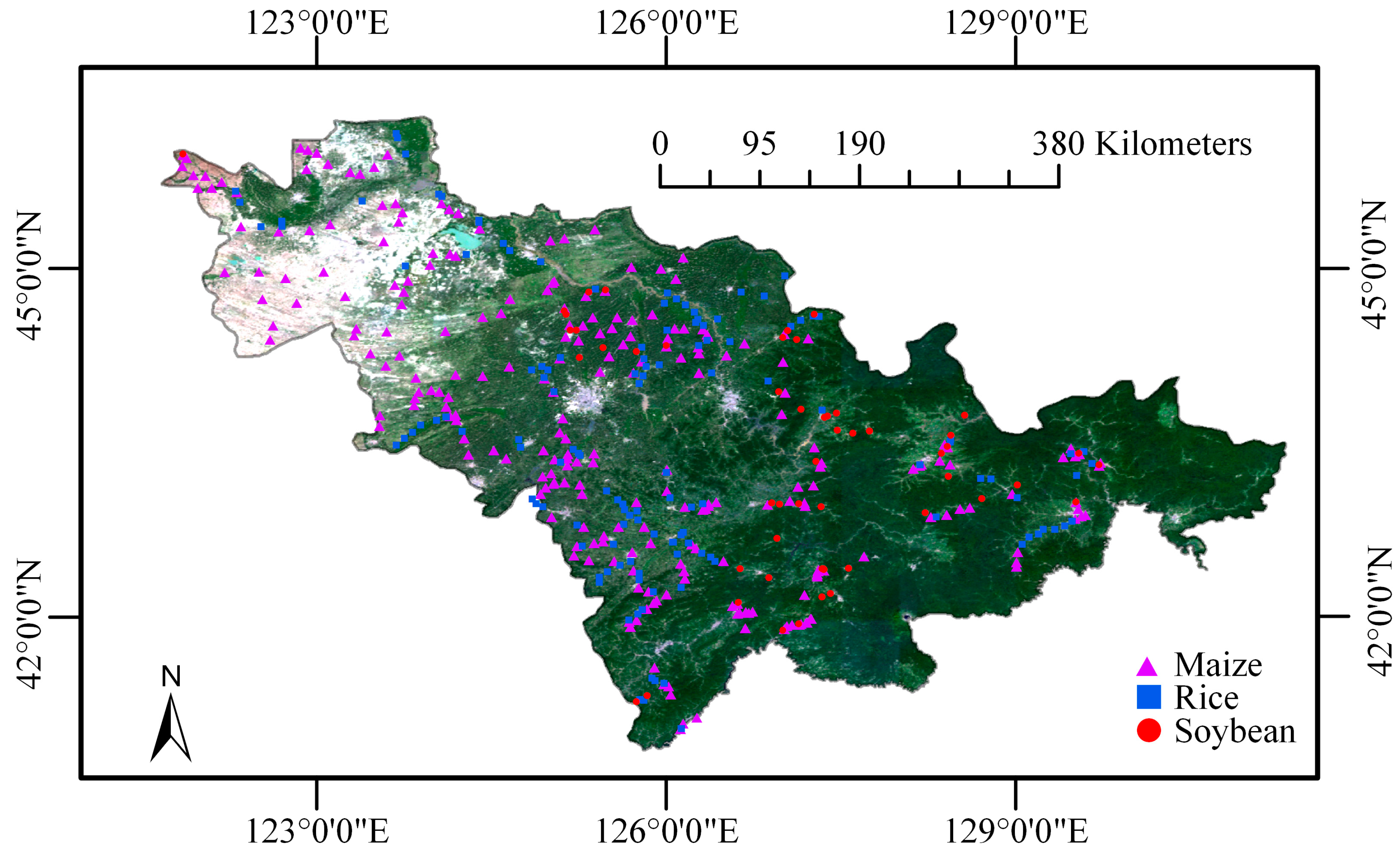
2.1. Study Area

The chosen study area is Jilin Province, located in northeast China, which includes the Yanbian Korean Autonomous Prefecture and eight prefecture-level cities. It covers approximately 190,000 km2 and is situated between 121°38′–131°19′E and 40°50′–46°19′N. (Figure 1). The study area boasts a vast expanse of diverse geomorphological features, characterized by a gentle northwestern terrain and a steep southeastern topography. Bordered by the sea, the area experiences a temperate monsoon climate, with regional changes in temperature, precipitation, and seasons. The mean temperature varies from lower than −11 °C in the winter to higher than 23 °C in the summer. The mean sunshine time per year is between 2259 and 3016 h. On average, the province receives 400 to 600 mm of precipitation annually, most of which falls in the east and is concentrated in the summer [32].
The natural resources and fertile soil of Jilin Province are abundant and particularly suited to the cultivation of maize, rice, and soya beans. All these crops have a growing season of about six months and are mono-annual (from late April to early October). The obtainability of water resources affects the distribution of crops across the province, with rice mainly grown in the Five River Basin, soybeans primarily grown in the eastern and central parts, and maize grown over the entire province [32]. Jilin Province is a key grain outcome and export foundation in China and has good conditions for developing grain production, known as the “hometown of soybeans” and the “golden corn belt”. The grain sowing area constitutes more than 85% of the total arable land, and the annual grain output is 16–25.1 million tons, making up approximately 4–5% of the country’s total grain production capacity, which has reached 25 million tons. Over the years, per capita grain production, sales volume, and export volume of grain have been among the highest in China [33].

2.2. Data

2.2.1. Reflectance Data

This study used two MODIS reflectance products, including the nadir BRDF-adjusted reflectance data (MCD43A4 V6) and the BRDF and albedo model parameter data (MCD43A1 V6). They are part of the MODIS BRDF/Albedo suite and provide observations of the anisotropic reflectance properties of the Earth’s surface, which is essential for various applications such as vegetation monitoring, land cover mapping, and climate modeling. The MODIS wavelengths and spatial resolution are listed in Table 1 [34]. The MCD43A4 V6 product is fitted using a BRDF to simulate the values as though they were observed in the nadir observation direction. The MCD43A1 V6 product offers the three model weighting parameters (i.e., isotropic, volumetric, and geometric parameters) for each of the MODIS bands. The products are generated using a combination of satellite data and modeling techniques [34]. The detailed data production process can be found in Appendix B.

2.2.2. Cropland Boundary Data

Cropland boundary data were provided by the annual MODIS MCD12Q1 V6 product [26]. MCD12Q1 is a land cover-type yearly global product from the MODIS sensors. This product provides global land cover classification data with a 500 m spatial resolution. The MCD12Q1 dataset is generated annually and contains information on various land cover types, such as urban areas, grasslands, croplands, wetlands, and forests. The MCD12Q1 product uses multiple classification schemes, and these classification schemes help scientists and decision-makers to better understand land cover dynamics, monitor changes, and assess the impacts of land use and land cover change on ecosystems, the climate, and human–environment interactions. We used the Annual International Geosphere–Biosphere Programme classification (land cover type 1) as a mask to select the cropland pixels. This mask selects pixels where not less than 60% of the area is cultured cropland. The detailed data production process can be found in Appendix C.

2.2.3. Field Sampling Data

Three field campaigns were conducted in Jilin Province in 2017 to obtain abundant and reliable prior knowledge and verification information on crop distribution in the study area. We employed a systematic field sampling site validation approach, which involved a sequence of progressive travel from the northwestern to the southeastern regions of Jilin Province. The field experiment was divided into three main stages: the first stage (1–6 September) was focused on the northwestern region of Jilin Province, primarily in Baicheng city and its surrounding areas; the second stage (12–21 September) involved targeting the central region of Jilin Province, mainly in Changchun city and its surrounding areas; the third stage (1–5 October) involved examining the southeastern region of Jilin Province, predominantly in Jilin city and its surrounding areas. After completing each phase of fieldwork, the team returned to the laboratory to process and verify the collected field data. Once the data had been validated, the subsequent fieldwork phase was initiated.
Prior to initiating field experiments, we roughly selected sampling sites indoors using high-spatial-resolution imagery (i.e., Sentinel-2) and approximate predicted crop types, favoring areas that were as large as possible, minimally disturbed, and easily accessible, while ensuring that all sampling sites were evenly distributed throughout the study area. Once all sampling points were identified, we used a portable global positioning system (GPS) to measure the geometric locations, validate the predetermined crop types, and document primary information for each cropland. GPS measurements were taken as close to the center of the field as possible, and preliminary data were recorded concurrently. Primary data mainly consisted of determined crop type, elevation, latitude, and longitude. In total, 258 corn, 132 rice, and 53 soybean sampling points were obtained. The distribution map of the field sampling points is shown in Figure 1.

3. Methods

3.1. Overall Processing

The whole process is illustrated in Figure 2. It can be divided into two parts: data preprocessing and supervised classification. Data preprocessing was aimed at obtaining composite images for crop mapping. The supervised classification aimed to evaluate the classification accuracy of random forest (RF), classification and regression trees (CART), support vector machine (SVM), and Naïve Bayes (NB) classifiers (Appendix D) using single- and multi-angle observation data.

3.2. Data Preprocessing

We assessed the potential of multi-angle observations for crop classification by utilizing both single- and multiple-angle-observation remote sensing data. The single-angle observation type was the MODIS nadir reflectance (MCD43A4 V6), referred to as NR (nadir reflectance). The multiple-angle observation type was the MODIS kernel-driven model parameters (MCD43A1 V6), referred to as MF (multi-angle observation factors).
We restricted the data to cover Jilin Province using one spatial filter and limited it to 2017 using one date filter. We employed all available MODIS NR and MF data from two distinct periods: the growth stage (day of year: 170–230) and the harvest stage (day of year: 231–291) [35]. Within each of these periods, we took the medians as temporal metrics for all band data (i.e., NR and MF) to provide to the classifiers. According to the literature [36], temporal metrics improved classification accuracy by 7%. Medians were used instead of means due to the non-symmetric error distribution [37,38]. Subsequently, we applied the MODIS MCD12Q1 V6 crop mask from 2017 to retain only crop pixels.
Finally, for the NR data type, we had 7 (bands) × 1 (direction) × 2 (phase) × 1 (temporal metric) = 14 classification indices to provide to classifiers for supervised classification. For the MF data type, we had 7 (bands) × 3 (direction) × 2 (phase) × 1 (temporal metric) = 42 classification indices to provide to classifiers for supervised classification.

3.3. Supervised Classification

The sampling points, together with their pixel values of the NR and MF, were randomly divided into modeling and validation groups in a ratio of 7:3. Then, a spatial join was performed by deleting the training samples within 1000 m of the validation samples to avoid a correlation due to the spatial autocorrelation of the predicted phenomena. The input sampling points were the same for each classifier. Four classifiers (RF, CART, SVM, and NB) provided by GEE were employed to assess the classification accuracy with the sampling points in Jilin Province. Finally, we classified crop types from composite images using trained classifiers and verified accuracy in terms of input data and classifier types. The input parameters are listed in Table 2.

4. Classification Results and Accuracy Assessment

The crop classification maps were drawn, and their areas were calculated. The classification results and accuracy of the four classifiers were compared concerning NR and MF data types.

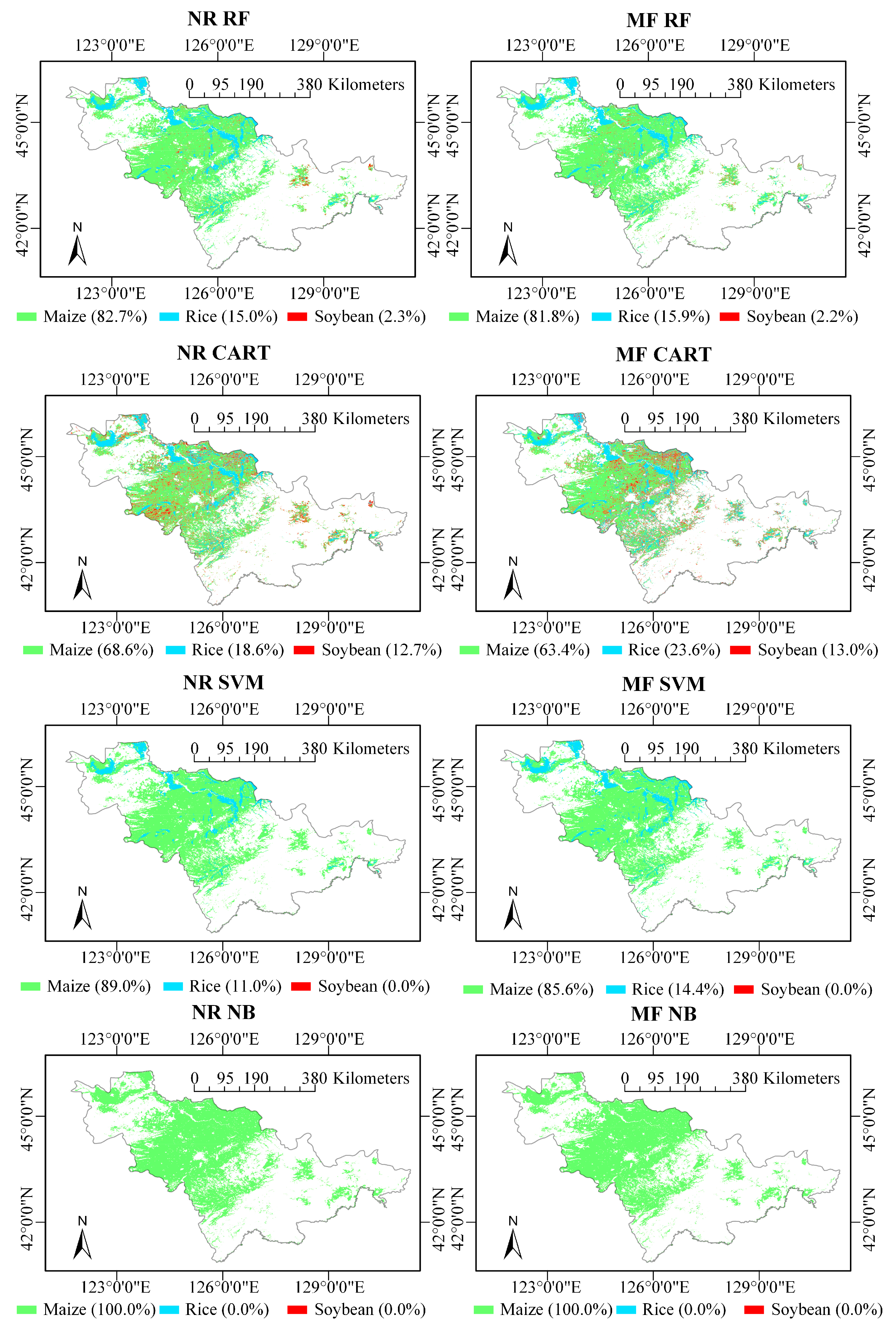
4.1. Classification Results

The crop mapping images are shown in Figure 3. The location of maize showed good consistency across the four classification results, while the location of soybean varied dramatically. Table 3 shows the crop area and corresponding classification accuracy. The choice of classifier had a more significant influence on the results than the input data did. Different classifiers produced significantly different classification results for the same classification data, with a maximum standard deviation of the maize area of 16,556.75 km2. In contrast, different classification data using the same classifier produced less different results, with the maximum standard deviation of maize area being 4083.54 km2. Notably, the SVM classifier was unable to classify soybean pixels using NR data, but it could classify them using MF data (despite accounting for a very small area). The NB classifier could not classify soybean and wheat pixels, regardless of whether NR or MF data were used.

4.2. Accuracy Assessment

The assessment of accuracy was conducted from three different perspectives, namely the accuracy of classification among classifiers, input data types, and crop types. The criteria used for evaluation were the overall accuracy and kappa coefficients. Overall accuracy is a metric that measures the proportion of correctly classified pixels to the overall amount of pixels in the image. It is a simple and easy-to-understand measure that offers an overall estimation of the robustness of the classification model. On the other hand, the kappa coefficient is a statistical measure that takes into account the agreement between the observed and expected classifications and corrects for the agreement that would be expected by chance. The kappa coefficient is in a range of −1 to 1, with 1 denoting perfect agreement, 0 denoting probability agreement, and −1 denoting total disagreement. Because it takes into account the agreement that would be predicted by chance, the kappa coefficient is a more reliable indicator than total accuracy is. Therefore, it is a more reliable measure of the performance of the classification model [42].

4.2.1. Evaluation of the Classifiers

Table 3 shows the classification result and accuracy (overall accuracy and kappa coefficient) of the RF, CART, SVM, and NB classifiers in terms of training and validation data. The four classifiers exhibited noteworthy differences in performance. The CART classifier held the highest training accuracy (overall training accuracy equaled 98.7%, and the training kappa coefficient equaled 0.977). The RF classifier held the highest overall validation accuracy (an overall validation accuracy of over 75% and a kappa coefficient of over 0.500). The SVM classifier (an overall accuracy of over 73.0% and a kappa coefficient of over 0.440) had lower training and validation accuracy than CART and RF did. The NB classifier had the worst accuracy among the four classifiers (overall validation accuracy equaled 54.9%, and the kappa coefficient equaled 0.000).

4.2.2. Evaluation of the Multi-Angle Observations

The use of multi-angle observation data could improve the classification accuracy of classifiers. Specifically, the accuracy of RF, CART, and SVM classifiers using MF data showed greater improvement than that using NR data. The overall validation accuracy of RF increased from 75.5% to 79.4%, and the validation kappa coefficient increased from 0.539 to 0.602. The overall validation accuracy of CART increased from 58.8% to 63.7%, and the validation kappa coefficient increased from 0.307 to 0.368. The overall validation accuracy of SVM increased from 73.5% to 77.5%, and the validation kappa coefficient increased from 0.450 to 0.542. However, the difference in accuracy caused by using NR and MF data (an overall accuracy of up to 4.9% and a kappa coefficient of up to 0.092) was relatively small compared to the difference caused by using different classifiers (an overall accuracy of up to 43.0% and a kappa coefficient of up to 0.977). Therefore, the choice of classifier was the dominant factor influencing classification accuracy (Table 3).

4.2.3. Accuracy Comparison among Crop Types

Table 4 and Table 5 show the producer accuracy (PA) and user accuracy (UA) measures of the training and validation datasets, respectively. Producer accuracy indicates the number of pixels properly classified in a specific class as a proportion of the total number of pixels in that class in the reference data. Producer accuracy assesses the classifier’s ability to accurately identify a specific class, indicating the probability that a certain class in the reference data (ground truth) is correctly classified in the image classification. This metric is also referred to as the commission error. A high producer accuracy indicates that the classifier effectively identifies a specific class, while a low producer accuracy suggests that the classifier may be misclassifying that class. User accuracy indicates the number of correctly classified pixels for a given class as a proportion of the total number of pixels in the image classification that are classified as that class. This metric is also known as the omission error. User accuracy evaluates the reliability of the classification for a specific class, indicating the probability that a certain class in the classified image corresponds to the same class in the reference data (ground truth). A high user accuracy indicates that the classification results for a specific class are reliable, while a low user accuracy suggests that the classifier may include pixels from other classes in the specific class [43].
The training dataset held higher PA and UA values than the validation dataset did, with mean values of 68.22% and 46.74%, respectively. Among the three crop types, maize held the highest accuracy (mean value averaged by method, input data type, training and validation, PA and UA; 83.42%), followed by rice (mean value averaged by method, input data type, training and validation, PA and UA; 62.05%), while soybean held the lowest accuracy (mean value averaged by method, input data type, training and validation, PA and UA; 26.97%). Notably, only the CART classifier produced reliable classification results for soybean.

5. Discussion and Conclusions

5.1. Discussion

5.1.1. Discussion of the Classifiers for Optical Data

The choice of classifier can greatly impact the accuracy of the classification [44,45]. In our case with MODIS optical images, the classifier is the dominant factor influencing the classification results, and the influence of NR or MF data on the results is small. Among the classifiers provided by GEE, RF has the highest validation accuracy, while CART has the highest training accuracy. SVM and RF show similar good performance for validation accuracy. NB shows the worst performance.
RF is generally considered the most accurate of the four classifiers provided by GEE. For example, a meta-analysis of 349 publications on GEE over the last decade shows that the RF algorithm is the most often employed classification classifier for satellite imagery [45]. In our case with optical data, RF shows the highest validation accuracy. However, CART holds higher training accuracy than RF does. This may be explained by several studies on crop mapping [46,47] and tree species mapping [48]. CART is suitable for areas with simple land cover categories and consistent spatial distribution, while RF is ideal for areas with complicated land cover types and disjointed spatial distribution [49]. Additionally, the quality of training samples can also affect the performance of classifiers [41]. The spatial resolution of MODIS of 500 m may not be sufficient for crop mapping studies compared to previous studies. Therefore, the components within a pixel may be more complex, and the mixed pixel effect may be more severe, affecting the quality of the training samples.
The noise in the training data also degenerates the SVM accuracy. Compared with the RF classifier [50], SVM may have a higher sensitivity to training data quality [51]. As a result, in line with the literature [52] on crop mapping that uses multi-temporal Sentinel-2 images, SVM has a lower accuracy than RF does. NB shows the worst performance because irrelevant features can easily fool it. Therefore, our research emphasizes the significance of selecting classifiers according to the intrinsic property of the study objective and the types of image data.

5.1.2. Discussion of the Multi-Angle Optical Observations

Multi-angle optical observation has been broadly utilized for Earth observation as it can capture BRDF signatures [53], and BRDF signatures have been shown to contribute to land cover classification [26,27] and vegetation architecture (e.g., LAI [29,30], LAD [28], and leaf size [31]) inversion. The variability of spectra between crops is much lower than the variability of spectra between land covers, increasing classification difficulty. However, the architecture (e.g., LAI, LAD, and leaf size) of crops may have a substantial difference, which can be well-expressed by BRDF signatures. Therefore, we propose using BRDF signatures captured by the multi-angle optical observation data for crop classification. Our results show that using multi-angle optical observations in most cases results in a moderate enhancement in the classification results compared with using only nadir reflectance data.

5.1.3. Discussion of the Accuracy Comparison among Crop Types

It has been reported that raising the number of training sets can result in a moderate improvement in classifier performance [40,41]. In our classification results, maize has the highest classification accuracy, followed by rice, while soybean has the lowest accuracy. This order corresponds to the number of points we sampled. However, when the sample size for training approaches a certain threshold, the impact of raising the sample size for training on the improvement of classification accuracy will progressively diminish and even reach a bottleneck. At this time, other methods should be employed to boost the classification accuracy, such as improving feature selection, adjusting classifier parameters, etc. [54]. Since the main crops are numerically dominant in the training sample, classifying crops that are not numerically dominant is a challenge.

5.2. Conclusions

We evaluated the potential of using BRDF signatures captured by multi-angle observation data for crop mapping using four machine learning classifiers provided by GEE and MODIS nadir BRDF-adjusted reflectance data and BRDF and albedo model parameter data. Some general conclusions are listed below:
  • Using BRDF signatures leads to a moderate improvement in classification results compared to using reflectance data from a single nadir observation direction.
  • Among the four classifiers, RF has the highest validation accuracy for crop mapping, followed by CART, SVM, and NB.
  • The selection of a classifier plays a crucial role in classification accuracy, regardless of whether NR or MF data is used.
Our study contributes to the utilization of multi-angle observation data for crop mapping. However, the usage of multi-angle remote sensing observations for crop mapping is still limited by a lack of data sources and the low spatial resolution of current multi-angle observation satellites. In addition, the use of multi-angle data will also lead to increased computational demands. The variation of input parameters may also influence the accuracy and ranking of the four classifiers.

Author Contributions

Methodology and writing—original draft preparation, Z.Z.; writing—review and editing, S.C. and T.Y.; supervision, J.-P.G.-E. and S.C.; funding acquisition Z.Z., S.C. and J.-P.G.-E. All authors have read and agreed to the published version of the manuscript.

Funding

This work was supported in part by the National Natural Science Foundation of China (No. 42201372), in part by the National Key Research and Development Program of China (No. 2020YFA0714103), in part by the Scientific and Technological Development Scheme of Jilin Province (No. 20210201138GX), and in part by the TOSCA program of the French space center (CNES).

Data Availability Statement

The Google Earth Engine can be assessed through the website (https://explorer.earthengine.google.com, accessed on 23 May 2023). The MCD43A1 product can be assessed through the website (https://developers.google.com/earth-engine/datasets/catalog/MODIS_006_MCD43A1, accessed on 23 May 2023). The MCD43A4 product can be assessed through the website (https://developers.google.com/earth-engine/datasets/catalog/MODIS_006_MCD43A4, accessed on 23 May 2023). The MCD12Q1 product can be assessed through the website (https://developers.google.com/earth-engine/datasets/catalog/MODIS_006_MCD12Q1, accessed on 23 May 2023). The random forest classifier provided by GEE can be accessed through the website (https://developers.google.com/earth-engine/apidocs/ee-classifier-smilerandomforest, accessed on 23 May 2023). The classifications and regression trees classifier provided by GEE can be accessed through the website (https://developers.google.com/earth-engine/apidocs/ee-classifier-smilecart, accessed on 23 May 2023). The support vector machine classifier provided by GEE can be accessed through the website (https://developers.google.com/earth-engine/apidocs/ee-classifier-libsvm, accessed on 23 May 2023). The Naïve Bayes classifier provided by GEE can be accessed through the website (https://developers.google.com/earth-engine/apidocs/ee-classifier-smilenaivebayes, accessed on 23 May 2023).

Acknowledgments

The authors express their gratitude to Eric Chavanon, Nicolas Lauret, and Jordan Guilleux at the University of Toulouse. The authors express their gratitude to Lisai Cao, Jian Li, and Peng Lu at the Jilin University.

Conflicts of Interest

The authors declare no conflict of interest.

Appendix A. Kernel-Based BRDF Model

The kernel-based BRDF model represents surface reflections as a linear combination of multiple models. To concentrate on surface directional reflection signatures, it separates direction-related terms from direction-independent terms in the model. The bi-directional reflectance factor, R(Ωi,Ωv), is expressed as follows:
R Ω i , Ω v = f isotropy   + f g e o m e t r y k g e o m e t r y Ω i , Ω v + f v o l u m e k v o l u m e Ω i , Ω v
Here, f represents direction-independent terms, including the isotropy scattering factor (fisotropy), geometry scattering factor (fgeometry), and volume scattering factor (fvolumn). The direction-dependent terms, k, include the geometry scattering kernel (kgeometry) and volume scattering kernel (kvolume), which are dependent on the direction of incidence, Ωi, and the direction of view, Ωv.

Appendix B. The Generation of the MCD43A1/MCD43A4 Product

The generation of the MCD43A1 BRDF/Albedo Model Parameters product involves three steps [55]: Collection of MODIS surface reflectance data: The MODIS sensors gather surface reflectance data at a 500 m spatial resolution in seven spectral bands. These data undergo preprocessing to correct for atmospheric effects, such as aerosols and water vapor. Then, to create the MCD43A1 BRDF/Albedo Model Parameters product, a 16-day composite of MODIS surface reflectance data is utilized. This composite is formed by selecting the highest-quality observations (i.e., values with optimal quality flags) from Terra and Aqua satellites over the 16-day period, taking into account factors such as cloud cover, view angle, and solar zenith angle. Finally, the BRDF model coefficients are estimated by fitting the model to the multi-date composite of MODIS surface reflectance data. This process, known as BRDF inversion, involves minimizing the difference between the observed and modeled reflectance by employing the kernel-based BRDF model.
The MCD43A4 NBAR (Nadir BRDF-Adjusted Reflectance) product is derived from the MCD43A1 BRDF/Albedo Model Parameters product. Once the BRDF model parameters are estimated, the NBAR product is generated by adjusting the surface reflectance data for the nadir view and solar zenith angles. This adjustment accounts for the anisotropic reflectance properties of Earth’s surface, providing a more consistent and accurate representation of surface reflectance [55].

Appendix C. The Generation of the MCD12Q1 Product

The generation of the annual global MCD12Q1 land cover type product involves a three-step process [26]: Remote sensing data are processed in 32-day cycles, aggregating measurements into summary data (studies including that in [56] have demonstrated that a minimum of 30 days is required to compile a dataset with minimal cloudiness impact). Remote sensing inputs for the 32-day database encompass land/water marks, skyline BRDF-adjusted reflectance, texture channels, vegetation indices, directional information, snow/ice cover, and surface temperature. Subsequently, the classification algorithm processes a series of twelve 32-day MOD12M databases and a global 1 km topographic database (EOS range) to generate seasonal land cover labels for data reduction. In the final classification phase, a sequence of 32-day databases and the earth observing system data and information system (EOSDIS) 1 km terrain database (MOD03) are provided as input to the classifier. The classifier then processes the 32-day databases and ancillary data using decision trees and neural network classification algorithms.

Appendix D. Supervised Machine Learning Classifiers in GEE

Four non-parametric machine learning classifiers provided by GEE, including random forest (RF, https://developers.google.com/earth-engine/apidocs/ee-classifier-smilerandomforest, accessed on 23 May 2023), classification and regression trees (CART, https://developers.google.com/earth-engine/apidocs/ee-classifier-smilecart, accessed on 23 May 2023), support vector machine (SVM, https://developers.google.com/earth-engine/apidocs/ee-classifier-libsvm, accessed on 23 May 2023), and Naïve Bayes (NB, https://developers.google.com/earth-engine/apidocs/ee-classifier-smilenaivebayes, accessed on 23 May 2023), were used to compare classification accuracy between single- and multi-angle observation data.
(1)
Random Forest
Random forest (RF) [57] is an ensemble learning method that combines multiple decision trees to improve the accuracy and robustness of a model. RF is famous for effectively handling large datasets with high dimensionality, providing a good balance between bias and variance, reducing the risk of overfitting by aggregating multiple decision trees, handling missing data and maintaining accuracy, and estimating feature importance. However, RF can be slow to train and predict with large trees and poor performance on imbalanced datasets [58,59].
(2)
Classification and Regression Trees
Classification and regression trees (CART) [60] is a decision tree learning technique that recursively splits the input data into subsets on the basis of the values of the input features, aiming to create pure leaf nodes (i.e., nodes containing only one class for classification or similar values for regression). CART is famous for capturing non-linear relationships and handling both categorical and continuous data. However, CART is prone to overfitting and sensitive to small changes in the data [59,61].
(3)
Support Vector Machine
Support vector machines (SVM) [62] is a supervised algorithm for binary classification tasks that finds the hyperplane that maximally separates the data into different classes. SVM is famous for handling high-dimensional data, its robustness to outliers, and its ability to capture non-linear relationships using kernel functions. However, SVM can be sensitive to the choice of kernel function and noise [59,63].
(4)
Naïve Bayes
Naïve Bayes (NB) [64] is a probabilistic algorithm that assumes independence between features given the class label. NB is famous for its fast training speed and for handling high-dimensional data. However, NB may not work well for correlated features [59,65].

References

  1. Khodadadzadeh, M.; Li, J.; Plaza, A.; Ghassemian, H.; Bioucas-Dias, J.M.; Li, X. Spectral–spatial classification of hyperspectral data using local and global probabilities for mixed pixel characterization. IEEE Trans. Geosci. Remote Sens. 2014, 52, 6298–6314. [Google Scholar] [CrossRef]
  2. Song, T.; Wang, Y.; Gao, C.; Chen, H.; Li, J. Mslan: A two-branch multi-directional spectral-spatial lstm attention network for hyperspectral image classification. IEEE Trans. Geosci. Remote Sens. 2022, 60, 5528814. [Google Scholar] [CrossRef]
  3. Mahlayeye, M.; Darvishzadeh, R.; Nelson, A. Cropping Patterns of Annual Crops: A Remote Sensing Review. Remote Sens. 2022, 14, 2404. [Google Scholar] [CrossRef]
  4. Zhen, Z.; Chen, S.; Yin, T.; Chavanon, E.; Lauret, N.; Guilleux, J.; Henke, M.; Qin, W.; Cao, L.; Li, J.; et al. Using the Negative Soil Adjustment Factor of Soil Adjusted Vegetation Index (SAVI) to Resist Saturation Effects and Estimate Leaf Area Index (LAI) in Dense Vegetation Areas. Sensors 2021, 21, 2115. [Google Scholar] [CrossRef] [PubMed]
  5. Abdelmoula, H.; Kallel, A.; Roujean, J.-L.; Gastellu-Etchegorry, J.-P. Dynamic retrieval of olive tree properties using Bayesian model and Sentinel-2 images. IEEE J. Sel. Top. Appl. Earth Observ. 2021, 14, 9267–9286. [Google Scholar] [CrossRef]
  6. Zhen, Z. Simulation de la Réflectance de la Végétation et Inversion des Propriétés Bio-optiques Basées sur un Modèle de Transfert Radiatif Tridimensionnel. Ph.D. Thesis, Université de Toulouse, Toulouse, France, 2021. [Google Scholar]
  7. Zhen, Z.; Gastellu-Etchegorry, J.-P.; Chen, S.; Yin, T.; Chavanon, E.; Lauret, N.; Guilleux, J. Quantitative Analysis of DART Calibration Accuracy for Retrieving Spectral Signatures Over Urban Area. IEEE J. Sel. Top. Appl. Earth Observ. 2021, 14, 10057–10068. [Google Scholar] [CrossRef]
  8. Duthoit, S.; Demarez, V.; Gastellu-Etchegorry, J.-P.; Martin, E.; Roujean, J.-L. Assessing the effects of the clumping phenomenon on BRDF of a maize crop based on 3D numerical scenes using DART model. Agric. For. Meteorol. 2008, 148, 1341–1352. [Google Scholar] [CrossRef]
  9. Zhen, Z.; Chen, S.; Yin, T.; Gastellu-Etchegorry, J.-P. Spatial Resolution Requirements for the Application of Temperature and Emissivity Separation (TES) Algorithm over Urban Areas. IEEE J. Sel. Top. Appl. Earth Observ. 2022, 15, 1–15. [Google Scholar] [CrossRef]
  10. Trevisan, R.G.; Shiratsuchi, L.S.; Bullock, D.S.; Martin, N.F. Improving yield mapping accuracy using remote sensing. In Precision Agriculture’19; Wageningen Academic Publishers: Wageningen, The Netherlands, 2019; pp. 1–16. [Google Scholar]
  11. Koh, K.; Hyder, A.; Karale, Y.; Kamel Boulos, M.N. Big Geospatial Data or Geospatial Big Data? A Systematic Narrative Review on the Use of Spatial Data Infrastructures for Big Geospatial Sensing Data in Public Health. Remote Sens. 2022, 14, 2996. [Google Scholar] [CrossRef]
  12. Gorelick, N.; Hancher, M.; Dixon, M.; Ilyushchenko, S.; Thau, D.; Moore, R. Google Earth Engine: Planetary-scale geospatial analysis for everyone. Remote Sens. Environ. 2017, 202, 18–27. [Google Scholar] [CrossRef]
  13. Jardim, A.M.d.R.F.; Araújo Júnior, G.d.N.; Silva, M.V.d.; Santos, A.d.; Silva, J.L.B.d.; Pandorfi, H.; Oliveira-Júnior, J.F.d.; Teixeira, A.H.d.C.; Teodoro, P.E.; de Lima, J.L. Using remote sensing to quantify the joint effects of climate and land use/land cover changes on the caatinga biome of northeast Brazilian. Remote Sens. 2022, 14, 1911. [Google Scholar] [CrossRef]
  14. Paoletti, M.E.; Haut, J.M.; Fernandez-Beltran, R.; Plaza, J.; Plaza, A.; Li, J.; Pla, F. Capsule networks for hyperspectral image classification. IEEE Trans. Geosci. Remote Sens. 2018, 57, 2145–2160. [Google Scholar] [CrossRef]
  15. Teodoro, P.E.; Teodoro, L.P.R.; Baio, F.H.R.; da Silva Junior, C.A.; dos Santos, R.G.; Ramos, A.P.M.; Pinheiro, M.M.F.; Osco, L.P.; Gonçalves, W.N.; Carneiro, A.M. Predicting days to maturity, plant height, and grain yield in soybean: A machine and deep learning approach using multispectral data. Remote Sens. 2021, 13, 4632. [Google Scholar] [CrossRef]
  16. Osco, L.P.; Junior, J.M.; Ramos, A.P.M.; Furuya, D.E.G.; Santana, D.C.; Teodoro, L.P.R.; Gonçalves, W.N.; Baio, F.H.R.; Pistori, H.; Junior, C.A.d.S. Leaf nitrogen concentration and plant height prediction for maize using UAV-based multispectral imagery and machine learning techniques. Remote Sens. 2020, 12, 3237. [Google Scholar] [CrossRef]
  17. Makhloufi, A.; Kallel, A.; Chaker, R.; Gastellu-Etchegorry, J.-P. Retrieval of olive tree biophysical properties from Sentinel-2 time series based on physical modelling and machine learning technique. Int. J. Remote Sens. 2021, 42, 8542–8571. [Google Scholar] [CrossRef]
  18. Ennouri, K.; Kallel, A. Remote sensing: An advanced technique for crop condition assessment. Math. Probl. Eng. 2019, 2019, 9404565. [Google Scholar] [CrossRef]
  19. Huang, X.; Li, S.; Li, J.; Jia, X.; Li, J.; Zhu, X.X.; Benediktsson, J.A. A multispectral and multiangle 3-D convolutional neural network for the classification of ZY-3 satellite images over urban areas. IEEE Trans. Geosci. Remote Sens. 2020, 59, 10266–10285. [Google Scholar] [CrossRef]
  20. Liang, B.; Liu, C.; Li, J.; Plaza, A.; Bioucas-Dias, J.M. Semisupervised Discriminative Random Field for Hyperspectral Image Classification. IEEE J. Sel. Top. Appl. Earth Observ. 2021, 14, 12403–12414. [Google Scholar] [CrossRef]
  21. Santana, D.C.; Teixeira Filho, M.C.M.; da Silva, M.R.; Chagas, P.H.M.d.; de Oliveira, J.L.G.; Baio, F.H.R.; Campos, C.N.S.; Teodoro, L.P.R.; da Silva Junior, C.A.; Teodoro, P.E. Machine Learning in the Classification of Soybean Genotypes for Primary Macronutrients’ Content Using UAV–Multispectral Sensor. Remote Sens. 2023, 15, 1457. [Google Scholar] [CrossRef]
  22. Baio, F.H.R.; Santana, D.C.; Teodoro, L.P.R.; Oliveira, I.C.d.; Gava, R.; de Oliveira, J.L.G.; Silva Junior, C.A.d.; Teodoro, P.E.; Shiratsuchi, L.S. Maize Yield Prediction with Machine Learning, Spectral Variables and Irrigation Management. Remote Sens. 2022, 15, 79. [Google Scholar] [CrossRef]
  23. Zhao, Q.; Yu, L.; Li, X.; Peng, D.; Zhang, Y.; Gong, P. Progress and trends in the application of Google Earth and Google Earth Engine. Remote Sens. 2021, 13, 3778. [Google Scholar] [CrossRef]
  24. Gastellu-Etchegorry, J.; Lauret, N.; Tavares, L.; Lamquin, N.; Bruniquel, V.; Roujean, J.; Hagolle, O.; Zhen, Z.; Wang, Y.; Regaieg, O. Correction of Directional Effects in Sentinel-2 and-3 Images with Sentinel-3 Time Series and Dart 3D Radiative Transfer Model. In Proceedings of IEEE International Geoscience and Remote Sensing Symposium, Kuala Lumpur, Malaysia, 17–22 July 2022; pp. 4563–4566. [Google Scholar]
  25. Bian, Z.; Qi, J.; Gastellu-Etchegorry, J.-P.; Roujean, J.-L.; Cao, B.; Li, H.; Du, Y.; Xiao, Q.; Liu, Q. A GPU-Based Solution for Ray Tracing 3-D Radiative Transfer Model for Optical and Thermal Images. IEEE Geosci. Remote Sens. 2022, 19, 1–5. [Google Scholar] [CrossRef]
  26. Strahler, A. MODIS land cover product algorithm theoretical basis document (ATBD) version 5.0. MODIS Doc. 1999, 42, 47. [Google Scholar]
  27. Jiao, Z.; Woodcock, C.; Schaaf, C.B.; Tan, B.; Liu, J.; Gao, F.; Strahler, A.; Li, X.; Wang, J. Improving MODIS land cover classification by combining MODIS spectral and angular signatures in a Canadian boreal forest. Can. J. Remote Sens. 2011, 37, 184–203. [Google Scholar] [CrossRef]
  28. Huang, W.; Niu, Z.; Wang, J.; Liu, L.; Zhao, C.; Liu, Q. Identifying crop leaf angle distribution based on two-temporal and bidirectional canopy reflectance. IEEE Trans. Geosci. Remote Sens. 2006, 44, 3601–3609. [Google Scholar] [CrossRef]
  29. Hasegawa, K.; Matsuyama, H.; Tsuzuki, H.; Sweda, T. Improving the estimation of leaf area index by using remotely sensed NDVI with BRDF signatures. Remote Sens. Environ. 2010, 114, 514–519. [Google Scholar] [CrossRef]
  30. Zhen, Z.; Chen, S.; Qin, W.; Yan, G.; Gastellu-Etchegorry, J.-P.; Cao, L.; Murefu, M.; Li, J.; Han, B. Potentials and Limits of Vegetation Indices With BRDF Signatures for Soil-Noise Resistance and Estimation of Leaf Area Index. IEEE Trans. Geosci. Remote Sens. 2020, 58, 5092–5108. [Google Scholar] [CrossRef]
  31. Goel, N.S.; Qin, W.; Wang, B. On the estimation of leaf size and crown geometry for tree canopies from hotspot observations. J. Geophys. Res. Atmos. 1997, 102, 29543–29554. [Google Scholar] [CrossRef]
  32. Han, C.; Chen, S.; Yu, Y.; Xu, Z.; Zhu, B.; Xu, X.; Wang, Z. Evaluation of Agricultural Land Suitability Based on RS, AHP, and MEA: A Case Study in Jilin Province, China. Agriculture 2021, 11, 370. [Google Scholar] [CrossRef]
  33. Wang, J. Analysis on the Grain-Production Growth and Influence Factors in Jilin Province; Jilin Agricultural University: Changchun, China, 2006. [Google Scholar]
  34. SINERGISE. Sentinel Hub. Available online: https://docs.sentinel-hub.com/api/latest/data/modis/mcd/#available-bands-and-data (accessed on 23 May 2023).
  35. You, N.; Dong, J.; Huang, J.; Du, G.; Zhang, G.; He, Y.; Yang, T.; Di, Y.; Xiao, X. The 10-m crop type maps in Northeast China during 2017–2019. Sci. Data 2021, 8, 1–11. [Google Scholar] [CrossRef]
  36. Mandal, D.; Kumar, V.; Rao, Y.S. An assessment of temporal RADARSAT-2 SAR data for crop classification using KPCA based support vector machine. Geocarto. Int. 2022, 37, 1547–1559. [Google Scholar] [CrossRef]
  37. Mitraka, Z.; Chrysoulakis, N.; Kamarianakis, Y.; Partsinevelos, P.; Tsouchlaraki, A. Improving the estimation of urban surface emissivity based on sub-pixel classification of high resolution satellite imagery. Remote Sens. Environ. 2012, 117, 125–134. [Google Scholar] [CrossRef]
  38. Useya, J.; Chen, S.; Murefu, M. Cropland Mapping and Change Detection: Toward Zimbabwean Cropland Inventory. IEEE Access 2019, 7, 53603–53620. [Google Scholar] [CrossRef]
  39. GEE. Available online: https://developers.google.com/earth-engine/guides/classification (accessed on 23 May 2023).
  40. Goldblatt, R.; You, W.; Hanson, G.; Khandelwal, A.K. Detecting the boundaries of urban areas in india: A dataset for pixel-based image classification in google earth engine. Remote Sens. 2016, 8, 634. [Google Scholar] [CrossRef]
  41. Shetty, S. Analysis of Machine Learning Classifiers for LULC Classification on Google Earth Engine; University of Twente: Enschede, The Netherlands, 2019. [Google Scholar]
  42. Richards, J.A.; Richards, J.A. Remote Sensing Digital Image Analysis; Springer: Berlin/Heidelberg, Germany, 2022; Volume 5. [Google Scholar]
  43. Jensen, J.R. Introductory Digital Image Processing: A Remote Sensing Perspective; Prentice-Hall Inc.: Hoboken, NJ, USA, 1996. [Google Scholar]
  44. Ghorbanian, A.; Kakooei, M.; Amani, M.; Mahdavi, S.; Mohammadzadeh, A.; Hasanlou, M. Improved land cover map of Iran using Sentinel imagery within Google Earth Engine and a novel automatic workflow for land cover classification using migrated training samples. ISPRS J. Photogramm. Remote Sens. 2020, 167, 276–288. [Google Scholar] [CrossRef]
  45. Amani, M.; Ghorbanian, A.; Ahmadi, S.A.; Kakooei, M.; Moghimi, A.; Mirmazloumi, S.M.; Moghaddam, S.H.A.; Mahdavi, S.; Ghahremanloo, M.; Parsian, S. Google earth engine cloud computing platform for remote sensing big data applications: A comprehensive review. IEEE J. Sel. Top. Appl. Earth Observ. 2020, 13, 5326–5350. [Google Scholar] [CrossRef]
  46. Shelestov, A.; Lavreniuk, M.; Kussul, N.; Novikov, A.; Skakun, S. Exploring Google Earth Engine platform for big data processing: Classification of multi-temporal satellite imagery for crop mapping. Front. Earth Sci. 2017, 5, 17. [Google Scholar] [CrossRef]
  47. Shelestov, A.; Lavreniuk, M.; Kussul, N.; Novikov, A.; Skakun, S. Large scale crop classification using Google earth engine platform. In Proceedings of the 2017 IEEE International Geoscience and Remote Sensing Symposium (IGARSS), Fort Worth, TX, USA, 23–28 July 2017; pp. 3696–3699. [Google Scholar]
  48. Kamal, M.; Jamaluddin, I.; Parela, A.; Farda, N.M. Comparison of Google Earth Engine (GEE)-based machine learning classifiers for mangrove mapping. In Proceedings of the 40th Asian Conference Remote Sensing, ACRS, Daejeon, Korea, 14–18 October 2019; pp. 1–8. [Google Scholar]
  49. Pan, X.; Wang, Z.; Gao, Y.; Dang, X.; Han, Y. Detailed and automated classification of land use/land cover using machine learning algorithms in Google Earth Engine. Geocarto. Int. 2022, 37, 5415–5432. [Google Scholar] [CrossRef]
  50. Mellor, A.; Boukir, S.; Haywood, A.; Jones, S. Exploring issues of training data imbalance and mislabelling on random forest performance for large area land cover classification using the ensemble margin. ISPRS J. Photogramm. Remote Sens. 2015, 105, 155–168. [Google Scholar] [CrossRef]
  51. Foody, G.M.; Pal, M.; Rocchini, D.; Garzon-Lopez, C.X.; Bastin, L. The sensitivity of mapping methods to reference data quality: Training supervised image classifications with imperfect reference data. ISPRS Int. J. Geo.-Inf. 2016, 5, 199. [Google Scholar] [CrossRef]
  52. Maponya, M.G.; Van Niekerk, A.; Mashimbye, Z.E. Pre-harvest classification of crop types using a Sentinel-2 time-series and machine learning. Comput. Electron. Agric. 2020, 169, 105164. [Google Scholar] [CrossRef]
  53. Li, J.; Chen, S.; Qin, W.; Murefu, M.; Wang, Y.; Yu, Y.; Zhen, Z. Spatio-temporal Characteristics of Area Coverage and Observation Geometry of the MISR Land-surface BRF Product: A Case Study of the Central Part of Northeast Asia. Chin. Geogr. Sci. 2019, 29, 679–688. [Google Scholar] [CrossRef]
  54. Bishop, C.M.; Nasrabadi, N.M. Pattern Recognition and Machine Learning; Springer: Berlin/Heidelberg, Germany, 2006; Volume 4. [Google Scholar]
  55. Schaaf, C.; Strahler, A.; Chopping, M.; Gao, F.; Hall, D.; Jin, Y.; Liang, S.; Nightingale, J.; Román, M.; Roy, D. MODIS MCD43 Product User Guide V005; University of Massachusetts Boston: Boston, MA, USA, 2021. [Google Scholar]
  56. Moody, A.; Strahler, A. Characteristics of composited AVHRR data and problems in their classification. Int. J. Remote Sens. 1994, 15, 3473–3491. [Google Scholar] [CrossRef]
  57. Breiman, L. Random forests. Mach. Learn. 2001, 45, 5–32. [Google Scholar] [CrossRef]
  58. Verikas, A.; Gelzinis, A.; Bacauskiene, M. Mining data with random forests: A survey and results of new tests. Pattern Recognit. 2011, 44, 330–349. [Google Scholar] [CrossRef]
  59. Lorena, A.C.; Jacintho, L.F.; Siqueira, M.F.; De Giovanni, R.; Lohmann, L.G.; De Carvalho, A.C.; Yamamoto, M. Comparing machine learning classifiers in potential distribution modelling. Expert Syst. Appl. 2011, 38, 5268–5275. [Google Scholar] [CrossRef]
  60. Breiman, L.; Friedman, J.; Stone, C.; Olshen, R. Classification and Regression Trees; Raton, B., Ed.; Taylor & Francis Ltd.: Oxfordshire, UK, 1984. [Google Scholar]
  61. Hastie, T.; Tibshirani, R.; Friedman, J.H.; Friedman, J.H. The Elements of Statistical Learning: Data Mining, Inference, and Prediction; Springer: Berlin/Heidelberg, Germany, 2009; Volume 2. [Google Scholar]
  62. Burges, C.J. A tutorial on support vector machines for pattern recognition. Data Min. Knowl. Discov. 1998, 2, 121–167. [Google Scholar] [CrossRef]
  63. Schölkopf, B.; Smola, A.J.; Bach, F. Learning with Kernels: Support Vector Machines, Regularization, Optimization, and Beyond; MIT press: Cambridge, MA, USA, 2002. [Google Scholar]
  64. Haykin, S. Neural Networks and Learning Machines, 3rd ed.; Prentice Hall: Upper Saddle River, NJ, USA, 2008. [Google Scholar]
  65. Hand, D.J.; Yu, K. Idiot’s Bayes—Not so stupid after all? Int. Stat. Rev. 2001, 69, 385–398. [Google Scholar]
Figure 1. The study area of the Jilin Province. The base map is the MODIS mosaic image of the growing season (day of year: 170–230). The RGB color is composed of bands 1 (red), 4 (green), and 3 (blue) with median reflectance. Point symbols in triangles, squares, and circles represent maize, rice, and soybean sampling points.
Remotesensing 15 02761 g001
Figure 2. The procedure of crop mapping. Dark parallelograms represent the input parameters. White rectangles represent the processes. NR: nadir reflectance data; MF: multi-angle observation factor data; RF: random forest; CART: classification and regression trees; SVM: support vector machine; NB: Naïve Bayes.
Remotesensing 15 02761 g002
Figure 3. Crop mapping images using the nadir reflectance data (NR) and multi-angle observation factor data (MF) classified by four classifiers (RF: random forest; CART: classification and regression trees; SVM: support vector machine; NB: Naïve Bayes) provided by the Google Earth Engine (GEE).
Remotesensing 15 02761 g003
Table 1. The channels (wavelengths) of the MODIS sensor. SWIR: short-wave infrared.
Band SequenceBandSpatial Resolution (m)Bandwidth (nm)
1Red500620–670
2NIR500841–876
3Blue500459–479
4Green500545–565
5N/A5001230–1250
6SWIR165001628–1652
7SWIR225002105–2155
Table 2. Input parameters for training per classifier. The values are determined by considering the GEE official help document [39] and the literature [40,41].
ParametersValues
Random forest (RF)
  The amount of decision trees to be created for rifles by class10
  The quantity of variables in each division0
  The smallest size of a terminal node1
  The percentage of input to the bag for each tree0.5
  Whether or not the out-of-bag mode should be used by the classifierFalse
Classification and regression trees (CART)
  The greatest amount of leaf nodes in each treeNone
  Create nodes only if the training set includes this many values or more1
Support vector machine (SVM)
  The process for making decisionsVoting
  The SVM typeC_SVC
  The kernel typeRBF
  Using or not using reducing algorithmsTrue
  The degree of the polynomialNone
  The gamma value in the kernel function0.5
  The coef0 value in the kernel functionNone
  The cost (C) parameter1
  The nu parameterNone
  The termination criterion toleranceNone
  The epsilon in the loss functionNone
  The class of the training data on which to train in a one-class SVMNone
Naïve Bayes (NB)
  Smoothing lambda0.000001
Table 3. Crop areas and classification accuracy. RF: random forest; CART: classification and regression trees; SVM: support vector machine; NB: Naïve Bayes. NR: nadir reflectance data; MF: multi-angle observation factor data. TA: overall training accuracy; VA: overall validation accuracy; TK: training kappa coefficient; VK: validation kappa coefficient.
ClassifierDataAreas (km2)TAVATKVK
MaizeRiceSoybean
RFNR90,835.5016,419.252542.2596.1%75.5%0.9290.539
RFMF89,836.5017,500.752459.7597.4%79.4%0.9530.602
CARTNR75,355.7520,469.0013,972.2598.7%58.8%0.9770.307
CARTMF69,580.7525,934.2514,282.0098.7%63.7%0.9770.368
SVMNR97,668.5012,128.500.0073.0%73.5%0.4420.450
SVMMF94,010.5015,786.000.5076.5%77.5%0.5310.542
NBNR109,797.000.000.0055.7%54.9%0.0000.000
NBMF109,797.000.000.0055.7%54.9%0.0000.000
Table 4. Producer accuracy (PA) and user accuracy (UA) of the training dataset. RF: random forest; CART: classification and regression trees; SVM: support vector machine; NB: Naïve Bayes. NR: nadir reflectance data; MF: multi-angle observation factor data.
ClassifierDataPAUA
MaizeRiceSoybeanMaizeRiceSoybean
RFNR98.4%93.8%90.5%94.7%98.7%95.0%
RFMF97.7%97.5%95.2%97.7%98.8%90.9%
CARTNR99.2%97.5%100.0%98.4%100.0%95.5%
CARTMF99.2%97.5%100.0%98.4%100.0%95.5%
SVMNR98.4%51.9%0.0%68.1%93.3%0.0%
SVMMF94.5%67.9%0.0%72.9%85.9%0.0%
NBNR100.0%0.0%0.0%55.7%0.0%0.0%
NBMF100.0%0.0%0.0%55.7%0.0%0.0%
Table 5. Producer accuracy (PA) and user accuracy (UA) of the validation dataset. RF: random forest, CART: classification and regression trees, SVM: support vector machine, NB: Naïve Bayes. NR: nadir reflectance data, MF: multi-angle observation factor data.
ClassifierDataPAUA
MaizeRiceSoybeanMaizeRiceSoybean
RFNR87.5%68.3%0.0%75.4%96.6%0.0%
RFMF87.5%78.0%0.0%77.8%88.9%0.0%
CARTNR62.5%53.7%60.0%66.0%78.6%14.3%
CARTMF69.6%61.0%20.0%70.9%80.6%6.2%
SVMNR98.2%48.8%0.0%67.9%95.2%0.0%
SVMMF94.6%63.4%0.0%72.6%89.7%0.0%
NBNR100.0%0.0%0.0%54.9%0.0%0.0%
NBMF100.0%0.0%0.0%54.9%0.0%0.0%
Disclaimer/Publisher’s Note: The statements, opinions and data contained in all publications are solely those of the individual author(s) and contributor(s) and not of MDPI and/or the editor(s). MDPI and/or the editor(s) disclaim responsibility for any injury to people or property resulting from any ideas, methods, instructions or products referred to in the content.

