Article

Improving Radar Data Assimilation Forecast Using Advanced Remote Sensing Data

1
Department of Atmospheric Sciences, Kyungpook National University, Daegu 41566, Republic of Korea
2
Kualanamu Meteorological Station, The Agency for Meteorology, Climatology, and Geophysics of the Republic of Indonesia (BMKG), Jl. Tengku Heran, Beringin, Deli Serdang 20552, Indonesia
*
Author to whom correspondence should be addressed.
Remote Sens. 2023, 15(11), 2760; https://doi.org/10.3390/rs15112760
Submission received: 7 April 2023 / Revised: 19 May 2023 / Accepted: 23 May 2023 / Published: 25 May 2023

Abstract

:
Assimilating the proper amount of water vapor into a numerical weather prediction (NWP) model is essential in accurately forecasting a heavy rainfall. Radar data assimilation can effectively initialize the three-dimensional structure, intensity, and movement of precipitation fields to an NWP at a high resolution (±250 m). However, the in-cloud water vapor amount estimated from radar reflectivity is empirical and assumes that the air is saturated when the reflectivity exceeds a certain threshold. Previous studies show that this assumption tends to overpredict the rainfall intensity in the early hours of the prediction. The purpose of this study is to reduce the initial value error associated with the amount of water vapor in radar reflectivity by introducing advanced remote sensing data. The ongoing research shows that errors can be largely solved by assimilating satellite all-sky radiances and global positioning system radio occultation (GPSRO) refractivity to enhance the moisture analysis during the cycling period. The impacts of assimilating moisture variables from satellite all-sky radiances and GPSRO refractivity in addition to hydrometeor variables from radar reflectivity generate proper amounts of moisture and hydrometeors at all levels of the initial state. Additionally, the assimilation of satellite atmospheric motion vectors (AMVs) improves wind information and the atmospheric dynamics driving the moisture field which, in turn, increase the accuracy of the moisture convergence and fluxes at the core of the convection. As a result, the accuracy of the timing and intensity of a heavy rainfall prediction is improved, and the hourly and accumulated forecast errors are reduced.

1. Introduction

With increasing supercomputing power, the resolutions of numerical weather prediction (NWP) models are increasing, depicting mesoscale features at a finer scale. This transition to higher-resolution NWP models has the potential to resolve 100 m scale convection and accurately predict and forecast intense and damaging rainfalls [1]. However, solely increasing the resolution of an NWP model does not ensure an accurate prediction. The routine assimilation of meteorological data is key to establishing the accuracy of an NWP, allowing the variables of the NWP model to align with real-world weather observations [2].
In forecasting extreme rainfall events, radar observations have brought prominent benefits to data assimilation systems in operational weather centers [3]. Radar reflectivity sensors identify high-resolution (±250 m) precipitation hydrometeors in clouds, and their radar radial velocities provide their motion information [4]. Xiao et al. (2005) introduced a radial velocity observation operator with the inclusion of rainwater terminal velocity and estimated the vertical velocity increment based on the dynamic balance of Richardson’s equation [5]. The results showed a reasonable wind and vertical velocity analysis, thus improving rainband movement and intensity predictions. The reflectivity from radar observations provides cloud property information for precipitating areas. Gao and Stensrud (2012) demonstrated a radar reflectivity operator that uses the background temperature from the NWP model to divide species of hydrometeors (snow, graupel, and hail), resulting in improved short-range forecasts [6]. Furthermore, Wang et al. (2013) introduced the in-cloud humidity radar reflectivity assumption wherein the environment is saturated in the presence of clouds or the radar reflectivity is higher than a certain threshold [7]. The assimilation of the water vapor from radar is supposed to provide a humid environment for maintaining convection. However, many studies show that this assumption is rudimentary and empirical, risking the overprediction of the water vapor content and rainfall in the early hours of the prediction [8]. Overcoming these problems is crucial since the storm environment is interrelated with the moisture and thermodynamic conditions of the atmosphere, which significantly impact the generation and dissipation of storms [9]. Research to alleviate the extra water vapor and spurious precipitation from radar was conducted, but uncertainty in overly drying the precipitation environment remains [10]. Recent studies have proved that the assimilation of humidity observations, such as satellite or global positioning system (GPS) data, with wind and hydrometeor observations from radar have improved the moisture fields and the initiation of forecast storms [11,12]. Furthermore, the combination of radar and satellite assimilation will overcome the limitation of the incapability of radar to provide information prior to the formation of precipitation particles.
Global positioning system radio occultation (GPSRO) observations provide water vapor information for use in an NWP with a high vertical resolution, absolute accuracy, and low noise. GPSRO data can retrieve a variety of data that can be used in NWP systems (e.g., refractivity, bending angle, and derived moisture and temperature). The assimilation of refractivity shows a good compromise when compared to the assimilation of bending angles or derived temperature and moisture [13,14]. Chang et al. (2022) showed that GPSRO refractivity can provide information about the high-moisture level (3–5 km), producing a better heavy rainfall forecast [15]. Boyaj et al. (2022) demonstrated the capability of GPSRO refractivity to enhance water vapor condensation and the top levels of ice, cloud, and rainwater, all of which improve hazardous rainfall predictions [16]. Cheng et al. (2018) showed that the assimilation of GPSRO refractivity alone enhances both the 24 h and 48 h regional rainfall forecasts, while the assimilation of GPSRO refractivity and conventional observations enhanced the 48 h forecast of light and heavy rain [17]. However, the GPSRO measurements usually have low spatiotemporal resolutions because they are random and facilitate limited observations. Therefore, assimilating the other potential water vapor observations alongside the GPSRO observations will assist in water vapor distribution.
The satellite uses infrared (IR) channels to observe the brightness temperature (BT; determined as the “radiance”), which provides continuous atmospheric state information about water vapor, temperature, winds, and cloud properties for the NWP, using the radiative transfer model (RTM) as the observation operator [18]. Satellite observations have better spatial and temporal coverage in areas where radar is not available, such as over oceans and in clear skies. Okamoto et al. (2019) and Xu et al. (2020) investigated the performance of assimilated all-sky radiance (ASR) values and showed the enhancement of hydrometeor and water vapor field information and an improvement in the accuracy of location and intensity rainfall predictions [19,20]. Zhang et al. (2019) assimilated hydrometeor and wind information from radar observations in addition to the all-sky satellite radiance values, demonstrating that all-sky satellite data increased warning leading times and improved the accuracy of mesocyclone track predictions, improving the accuracy and providing longer lead times for the mesocyclone [21]. Wang et al. (2020) obtained simultaneous satellite and radar data, establishing that satellite data assimilation enhanced large-scale temperature and moisture variables, while the addition of radar data assimilation enhanced the wind field and hydrometeors in the precipitation area [22]. These improvements caused the assimilation to spin up faster, strengthening the initial intensity of the precipitation. Jones et al. (2020) combined radar and conventional observation data together with all-sky satellite radiances, providing improved analyses and forecasts of storm environments [23].
The storm morphology and evolution within an NWP are sensitive to the wind fields. The satellite-derived winds or atmospheric motion vectors (AMVs) offer tropospheric wind with high levels of spatial and temporal coverage that radar radial velocity or conventional data cannot observe. AMVs are mainly used to identify synoptic scale airflows, but AMVs can also be used to identify mesoscale winds induced by convective clouds [24]. It is important for the mesoscale flow fields to be resolved for high-impact, convective-scale forecast events [25]. Zhao et al. (2021) showed that the assimilation of AMVs enhanced the initial wind fields at the sites of upper-level divergence and low-level convergence around the storm, causing a positive impact on the timing and intensity of heavy rainfall [26]. Kim et al. (2018) discussed the potential benefits of AMVs over East Asia, and the resulting Himawari-8 AMVs reduced forecast errors [27].
The primary objective of this study is to improve the accuracy of radar data assimilation using advanced remote sensing data. The simultaneous assimilation of radar data with all-sky radiance, GPSRO refractivity, and AMVs is introduced in this study. The impacts of GPSRO refractivity and satellite all-sky radiances on improving the water vapor fields and satellite AMVs in updating real-world atmosphere flows are investigated when combined with radar data. The contributions are assessed based on a summertime precipitation forecast using the weather research forecasting (WRF) three-dimensional variational data assimilation (3DVAR) system. Section 2 and Section 3 describe the details of the experimental methods, data, and design. Section 3 analyzes the increments and water vapor dynamics in the initial condition, as well as the result of the rainfall forecast and the verification statistics. Section 4 presents the conclusion of the study results and a discussion of areas of further study.

2. Methodology

2.1. WRF 3DVAR Data Assimilation System

The weather research forecasting data assimilation (WRFDA) system with a three-dimensional variational data assimilation (3DVAR) framework was utilized in this study [28,29]. The 3DVAR system produces a multivariate incremental analysis for relative humidity, temperature, pressure, and wind. The incremental system minimizes a cost function J x , which is essentially defined as the weighted measure of the misfit between the model trajectory and the available observations over a fixed assimilation interval, weighted by the uncertainties in the respective data [30].
J x = J b x   +   J o x = 1 2 x x b T B 1 x x b +   1 2 y 0 H x T R 1 y H x
J o x and J b x are the cost functions obtained from the observations and background, respectively. The x, x b , y 0 , B , H , and R variables represent the analysis field, first guess, observation, background error (BE) covariance matrix, nonlinear observation operator, and observation error covariance matrix, respectively. The BE covariance matrix was produced using 12 h and 24 h forecasts during the summer season from 1 August to 30 September 2020, based on the method of the National Meteorological Center (NMC) [31].

2.2. Satellite Radiance Observation Operator

A radiance observation operator is required to calculate simulated radiance data from the model state vector. The Community Radiative Transfer Model (CRTM) from the United States Joint Center for Satellite Data Assimilation (JCSDA) was used as the radiance observation operator [32]. The CRTM contains various modules: a gaseous transmittance model, surface emission and reflection model, cloud and aerosol scattering model, and a radiative transfer solver. A variational bias correction (VarBC) [33,34,35,36] was performed when assimilating the radiance data.
The radiance observation error can be defined as standard deviation of the observation minus background departure (OMB), which can be described by the cloud parameter ( C A ). The C A formulation, developed by Okamoto et al. [37,38], can be written as:
C A = B B c l r + O B c l r 2    
where O, B, and B c l r are the radiance observation, simulated all-sky radiance, and simulated clear-sky radiance, respectively. In this study, the all-sky radiance observation error was estimated using a pre-calculated look-up table (LUT) approach based on a cloud situation using C A . C A and the standard deviation of the OMB statistics were calculated during August 2020 every six hours. The   C A   was split into bins of 1 K, and the standard deviation of the OMB was computed for each C A bin. The observation error was produced by fitting the C A bins and the standard deviation of the OMB using polynomial regression, which is written as:
  y = a x + b x 2 + c x 3 + d x 4 + e x 5 + f      
where y, as the polynomial fit, represents the observation error, x is the cloud parameter ( C A ), and af are the coefficients of the polynomial fit. Before reaching a maximum STD of the OMB value, the observation error follows these polynomial fit values and the rest remain constant with the highest polynomial fit value.

2.3. GPSRO Refractivity Observation Operator

The GPSRO technique utilizes GPS radio signals received from low Earth orbit (LEO) satellites to measure the amplitude and phase of the signals. These measurements, together with the precise knowledge of the position and velocity of the LEO and GPS satellites and the assumption of a spherically symmetric refractive index, compute the vertical profiles of the ray bending angle and retrieve the atmospheric refractivity (N) through the able transform method [39]. After the ionospheric effect is removed in the neutral atmosphere, the equation of refractivity (N) as a function of the water vapor pressure e (hPa), temperature T (K), and pressure P (hPa) and can be expressed as follows [40]:
  N = 77.6 P T + 3.73 × 10 5 e T 2      
To assimilate the refractivity, the model variables of temperature, pressure, and water vapor field were interpolated into the locations of the GPSRO observations.

3. Data and Experimental Setup

3.1. Observation Data

Radar reflectivity and radial velocity were obtained from the S-band radars of the Korea Meteorological Administration (KMA) (Figure 1a). The radar data were quality controlled using the Kyungpook National University (KNU) fuzzy logic algorithm [41], which removed the anomalous propagation (AP) and non-precipitating areas of electromagnetic waves. The procedure included a quality check on a plan position indicator (PPI) before conversion to a constant altitude PPI (CAPPI). The radar data were interpolated into the same resolution and size of the NWP domain. Therefore, the resolution of the radar data for domain 2 was 3 km, and the resolution of the radar data for domain 1 was 1 km. The vertical resolution for the radar data was set to 200 m.
The satellite observations used in this study were obtained from the GK-2A geostationary satellite. In this study, channels 8 to 10 (6.3, 6.9, and 7.3 µm) were used for all-sky radiance observation. These channels are the water vapor wavelengths that are sensitive to the water vapor in the middle to upper troposphere [42].
The GPSRO is a limb measurement based on Snell’s law of refraction. GPSRO sounding data were obtained from various missions: the Constellation Observing System for Meteorology, Ionosphere and Climate 2 (COSMIC 2), the Meteorological Operational Satellite Program (Metop, A-B), Paz, TanDEM-X (Tdx), TerraSAR-X (Tsx), and the Korea Multi-Purpose Satellite-5 (Kompsat5) with an atmospheric occultation profile with moisture information 2 (wetPf2), which consists of the refractivity associated with the location point (longitude and latitude) and the height of tangent point.
The GK2A AMVs are defined as the outputs of the atmospheric movements obtained by tracking clouds or water vapor fields with satellites. To calculate the motion vectors, three consecutive images are typically used in a time series. The AMVs used in this study were from the channels shortwave infrared (SWIR—3.8 μm), water vapor (WV—6.3, 6.9, and 7.3 μm), and infrared (IR—10.5 and 11.2 μm), with observation errors of 3.26, 4.62, 3.86, 4.94, 4.29, and 4.32 m s−1, respectively. The AMVs were quality-checked before being input into the 3DVAR data assimilation. Only AMVs with a quality indicator (QI) above 0.85 were assimilated. For the horizontal resolution, the GK-2A AMVs had a resolution of 32 × 32 km.
The radiosonde, wind profiler, and automatic weather station (AWS) observation data were obtained from the stations operated by the KMA (Figure 1b). The AWS precipitation data were interpolated into the same resolution and domain size as the model grid.

3.2. Event Overviews

Four cases of heavy rainfall over the Republic of Korea during the summer were chosen to study the impact of multiscale data assimilation into NWP model forecasts. The four characteristics of the selected cases, the mesoscale precipitation induced by the Changma front (Case 1), convective systems along the Changma front (Case 2), the mesoscale convective systems (MCSs) along the Changma front (Case 3), and the convective band (Case 4), are shown in Table 1 with the forecast period.
In Case 1, at 00 UTC on 9 August 2020, the Changma front propagated from the southwest to the northeast, and a large amount of water vapor was brought by a low-level jet (purple zones) (Figure 2a). The Changma front caused heavy rainfall, with 53.0 mm of hourly rainfall recorded in Osan, Gyeonggi Province (Figure 2e). The accumulation of 9 h of rainfall reached 107.32 mm in Pogog-eup, Gyeonggi Province.
In Case 2, at 0000 UTC on 15 August 2020, it can be seen that high pressure extended westward over the North Pacific and low pressure extended westward over Northeast China, inducing the Changma front, which approached eastward over the Republic of Korea (Figure 2b). The hourly rainfall peaked 44.0 mm in Gangnam, Gyeonggi Province, at 2200 UTC, 15 August 2020 (Figure 2f). The 12 h precipitation peak reached 114.80 mm in Hoengseong, Gyeonggi Province.
In Case 3, at 1200 UTC on 2 August 2020, the low pressure over Northwest China approached the southeast region and met the high pressure from the North Pacific, causing the Changma front (Figure 2c). The MCS occurred near the front that was initiated by the low-level jet (Figure 2c). Along the low-level jet, the MCS propagated from north to south, causing heavy rainfall over Gangwon, Gyeonggi, Chungcheongnam, and Chungcheongbuk. The hourly precipitation reached 50.0 mm in Baekhak-myeon, Gyeonggi Province, at 0700 UTC 2, August 2020 (Figure 2g). The accumulation of 27 h of rainfall reached 294.64 mm in Gyeonggi Province.
On 11 July 2021 (Case 4), low pressure approached from East China and high pressure approached over the North Pacific (Figure 2d). In Case 4, the synoptic factor was weak because it was caused by the local convective systems over Gyeonggi Province. This convective system caused the peak hourly precipitation of 52.5 mm at 0700 UTC, 11 July 2020 (Figure 2h), and the 12 h precipitation peak reached 72.87 mm in Buknae, Gyeonggi Province.

3.3. Experimental Setup and Design

In this study, the WRF model was utilized as an NWP. The WRF model offers open-source code, is flexible, and has a wide range of meteorological applications. The WRF features a compressible and non-hydrostatic mass coordinate system [43].
For every case, the WRF model used three nesting domains (D01, D02, and D03) with resolutions of 9 km, 3 km, and 1 km, respectively (Figure 3). Regarding cases related to the Changma front, Cases 1 and 2 had the same domain configuration because both cases predicted a short time period (9 h and 12 h), while Case 3 was developed in larger domain area to provide more data since this case predicted a long period time (27 h) (Figure 3, Table 1). For the convective case, the domain configuration of Case 4 was designed with a focus on the location of the rainfall event. The vertical level had 60 η model layers, and the highest level was 50 hPa. The initial and lateral boundary conditions used the NCEP/FNL (National Centers for Environmental Prediction/Final Analysis) with a resolution of 1° × 1°, which was developed by the National Centers for Environmental Prediction/National Centers for Atmospheric Research (NCEP/NCAR). In the WRF forecast simulations, the Kain–Fritsch scheme was applied for domains 1 and 2 [44]. For all domains, the WRF double moment 6 class (WDM6) scheme [45], the unified Noah land surface model [46], the YSU scheme [47], and the rapid radiative transfer model (RRTM) longwave scheme and the Dudhia shortwave scheme [48] were employed for cloud microphysics, land surface, planetary boundary layer, and the atmospheric radiation process, respectively. All model parameterizations and vertical levels were the same in each domain configuration.
To understand and analyze the strengths and limitations of each moisture information data type (radar, satellite, and GPSRO) and AMV, the sequence of the four experiments (CTRL, RQV, GPS + ASR, GPS + ASR + AMV) was confirmed (Table 2), and the increment analyses and prediction from each experiment were then compared with the available observations. CTRL experiment assimilated the AWS, radiosonde, wind profiler, and radar measurements. RQV, GPS + ASR, and GPS + ASR + AMV were identical to CTRL except that RQV additionally assimilated the in-cloud water vapor from radar reflectivity. GPS + ASR was identical to RQV with the addition of GPSRO refractivity and satellite all-sky radiances assimilation, and GPS + ASR + AMV was identical to GPS + ASR and was combined with the assimilation of AMVs. All assimilation experiments were conducted with continuous cycling in a 30 min window during a 3 h period (Figure 3). Satellite all-sky radiances and the GPSRO refractivity were assimilated into D01, D02, and D03. This method allows more data to be assimilated and may improve the synoptic scale analysis. The AWS, radar, wind profiler, and radiosonde data were assimilated into D02 and D03.

3.4. Verification Method

This study selected a couple of verification statistics to objectively evaluate the performances of the forecast models. AWS observations were utilized for the verification. The quantitative verification was performed using bias and root mean square error (RMSE) metrics, which can be defined as shown below. In Case 3, the BT observation reveals that:
Bias   = 1 N i   = 1 N   P i   O i  
  RMSE   = 1 N i   = 1 N P i   O i 2  
where N represents the total number of data, P i represents the prediction, and O i represents the observation. Bias describes whether the forecast models underpredict (BIAS < 0) or overpredict (BIAS > 0) events. The RMSE determines the standard deviation of the forecast errors.
Precipitation occurrences can be verified using four categories (Hits, False Alarms, Misses, and Correct Negatives), as shown by the contingency table. The accuracy (AC) describes the quantity of correct forecasts, as defined in Equation (7). A value of one is a perfect score.
Accuracy   = Hits   +   Correct   Negatives Total
The critical measure index (CSI) determines the ratio of correct predictions. The ratio of the prediction becomes higher when Hits occurs but becomes lower when Misses and False Alarms occur. The best CSI score is a value of one.
CSI   = Hits Hits   +   Misses   +   False   Alarms
The equitable threat score (ETS) is comparable with CSI, but the ETS also considers the random chance of Hits. The ETS perfect score is a value of one.
Hits random = Hits   +   Misses Hits   +   False   Alarms Total
  ETS   = Hits     Hits random Hits   +   Misses   +   False   Alarms     Hits random
To objectively evaluate the precipitation pattern, a pattern correlation (PC) was performed. The PC is expressed in Equation (11):
R patt _ cor = i   = 1 N X obs , i X ¯ obs X pred , i X ¯ pred σ obs σ pred
where N is the number of data, X o b s and X ¯ o b s are the precipitation observation and the mean of the precipitation observation, respectively, X p r e d and X ¯ p r e d are the precipitation forecast and the mean of the precipitation forecast, respectively, and σ o b s   and σ p r e d are the standard deviation of the precipitation observation and forecast, respectively. The highest accuracy is a value of one.

4. Results

4.1. Analyzing the Increments of Initial Fields

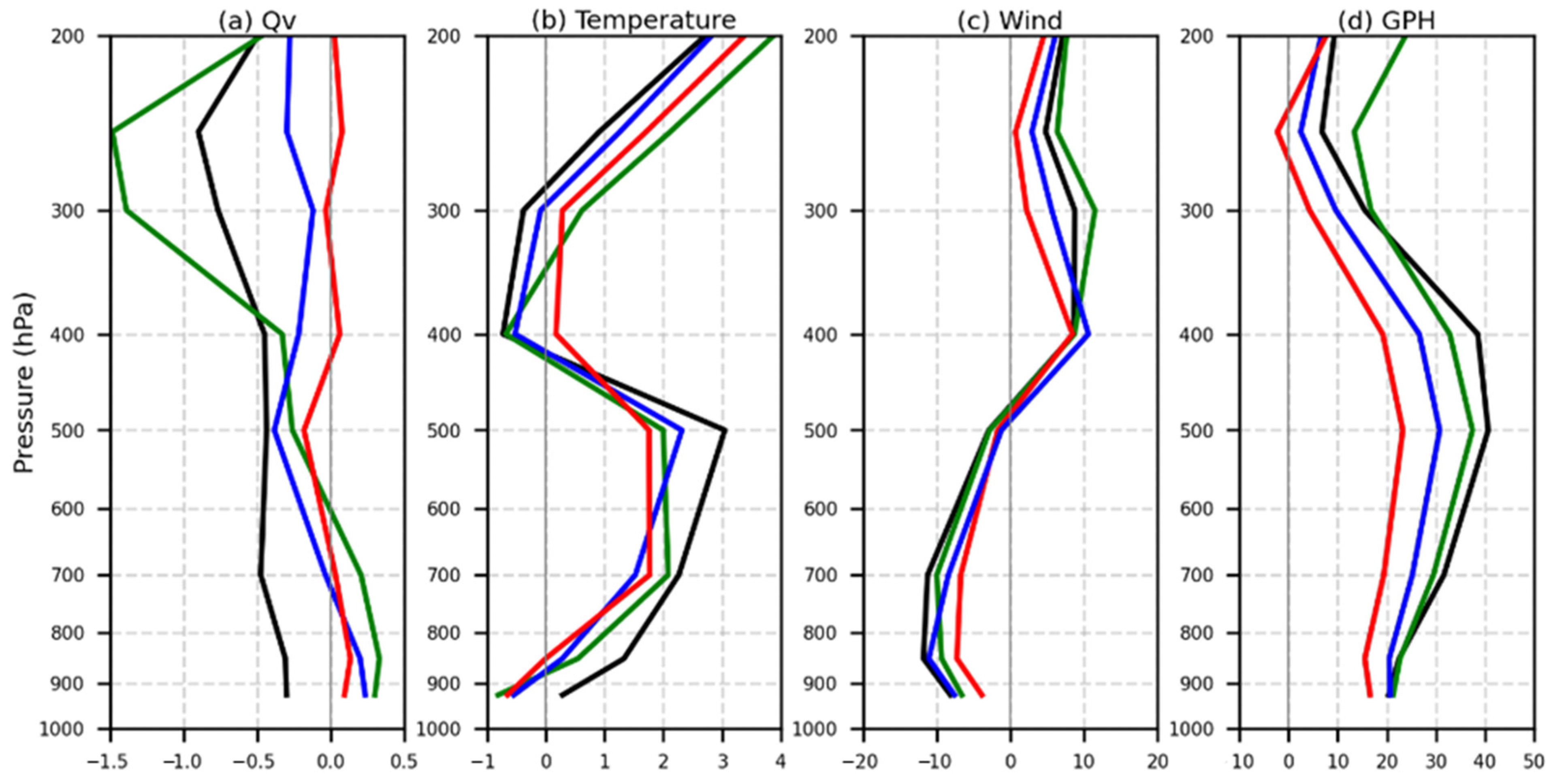
To improve the fidelity of the numerical model simulations, the initial analysis fields should demonstrate similarity to the real world. Thus, the contribution of each simulation to improving the rainfall forecast can be established by analyzing the increments of the initial fields. An enhancement in water vapor content is associated with changes in the thermodynamic process that may contribute to wind field changes. In addition, changes in dynamic winds should primarily result from changes in the pressure fields. Thus, understanding that the wind, pressure, and temperature fields are modified in the initial field through each simulation is crucial. The horizontal and vertical increments were analyzed at the end of the cycling assimilation window to evaluate the impact of each simulation. 
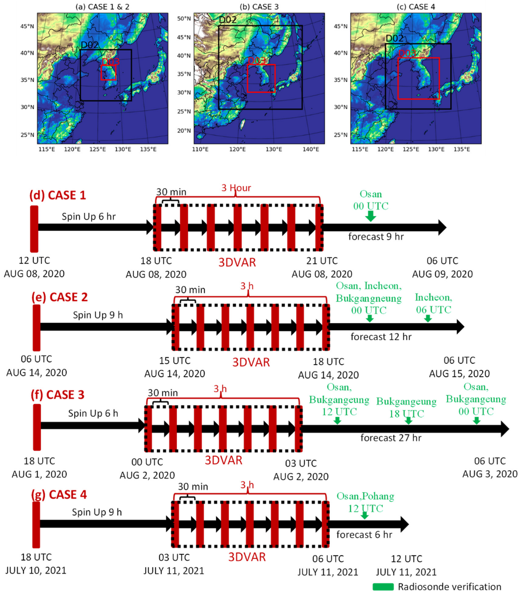
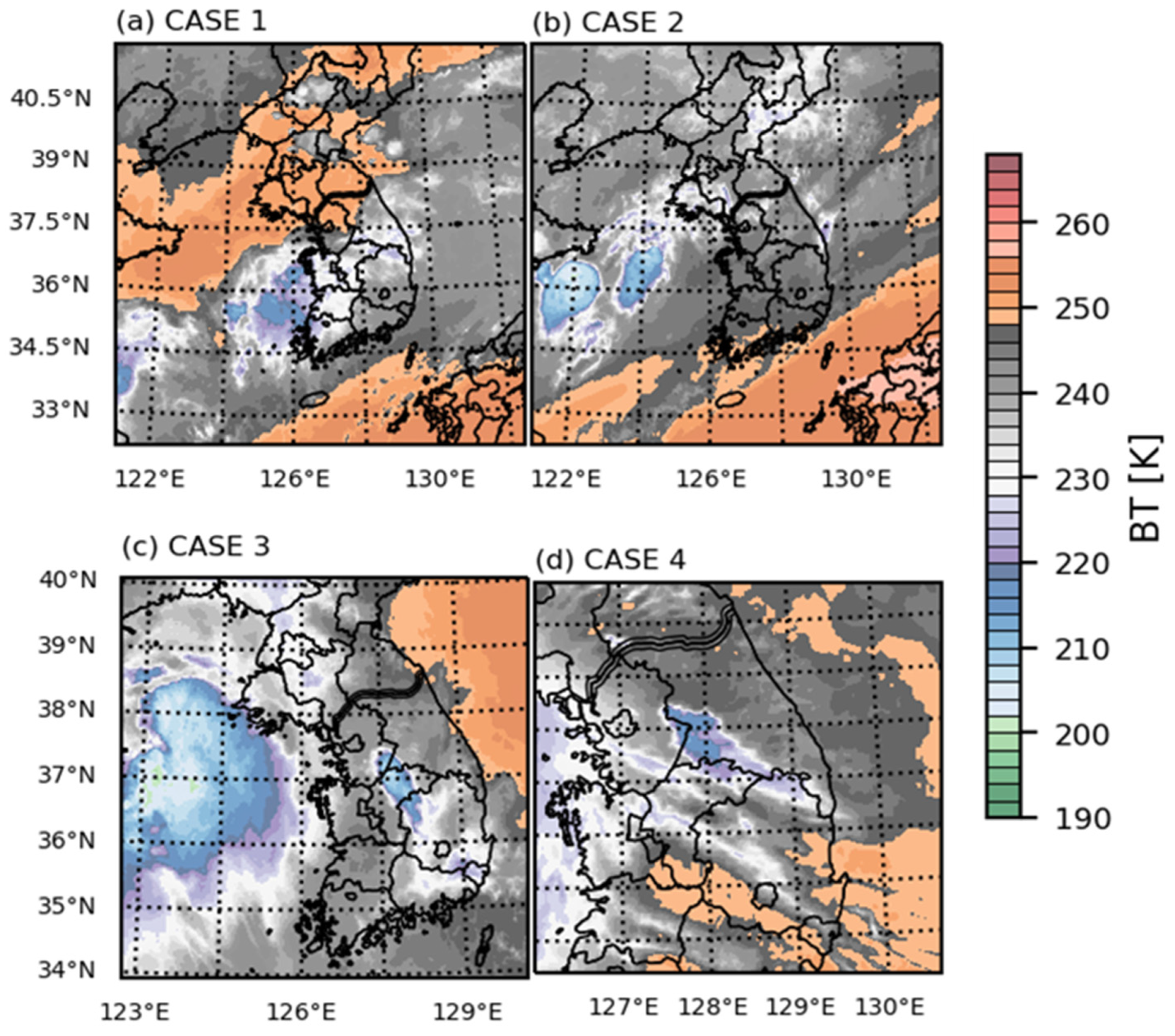
Figure 4 displays the satellite observations of the brightness temperature (K) for the channel of a 6.9 μm water vapor wavelength at the last data assimilation cycle for each case. Figure 5, Figure 6 and 
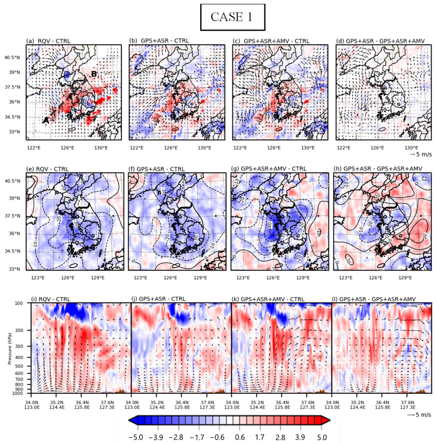
Figure 7 show the increment of the water vapor mixing ratio (g kg−1) overlaid by wind (m s−1) at 850 hPa, the perturbation pressure (hPa) overlaid by the geopotential height (meter) at 850 hPa, and the vertical (A-B line) perturbation temperature (K) overlaid by the wind (u, w × 5 m s−1) for Cases 1, 3, and 4, respectively. Domain 2 was used for domain analysis increments, but domain 2 was cropped on Cases 3 and 4, focusing on the location of the rainfall systems for a clear picture. The 850 hPa level was chosen because this level is generally used to identify air masses and to locate warm and cold fronts.
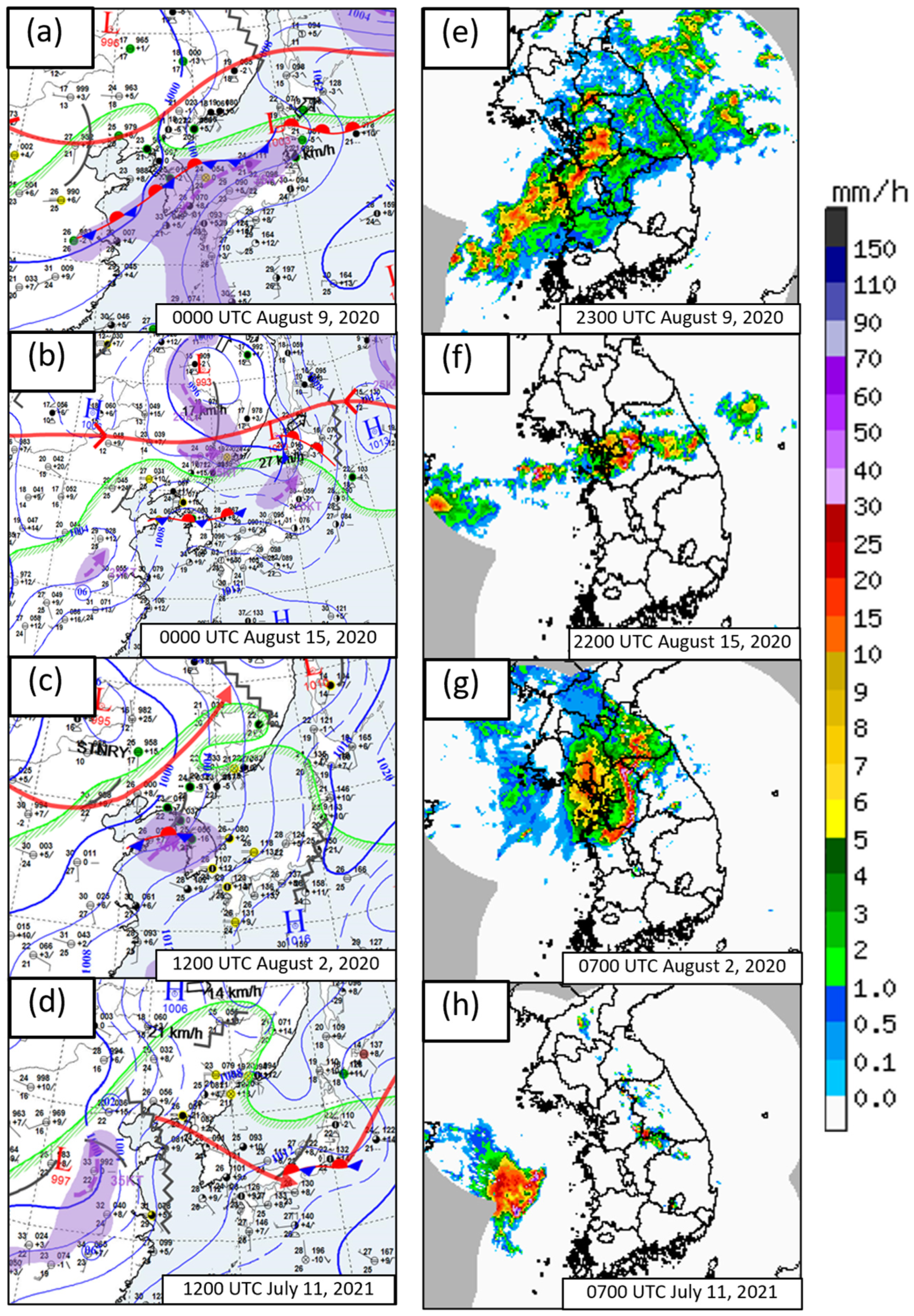
In Case 1, the BT observation from the satellite shows convective elements over the east of the Yellow Sea, denoted by BT < 220 K, which are associated with moister atmospheric conditions (Figure 4a). RQV showed a strong magnitude of the positive water vapor mixing ratio in the larger areas over the east of the Yellow Sea at approximately 4.5 g kg−1 (Figure 5a). Such an increment may cause the overprediction of rainfall. GPS + ASR also increased the water vapor mixing ratio, which was approximately 4.5 g kg−1, in smaller areas compared to RQV (Figure 5b). GPS + ASR + AMV showed similarity with GPS + ASR in the increment of the water vapor mixing ratio over the convective area (Figure 5c), as indicated by small differences in the water vapor content between GPS + ASR + AMV and GPS + ASR (Figure 5d). Clearly, the positive water vapor increments in RQV, GPS + ASR, and GPS + ASR + AMV were associated with increases in blowing wind from the northwest to the Yellow Sea of approximately 2 m s−1, 2 m s−1, and 4.5 m s−1, respectively, enhancing the convergence (Figure 5a–c). This result was mainly caused by the intensified low-pressure regions over the eastern Yellow Sea (Figure 5e–g). However, there was a slight gradient of perturbation pressure in GPS + ASR at approximately 35.8°N 124°E before the convection area was reached (Figure 5f). This increment changed the wind direction, moving from northwesterly to easterly, and weakened the convergence over the convection area (Figure 5b). GPS + ASR + AMV showed the most intensification of low perturbation pressure over the convection area at approximately 4.5 hPa (Figure 5g), increasing the wind convergence (Figure 5c). In addition, the highest gradient of geopotential height in GPS + ASR + AMV was mostly observed in the northwest, with strong northwesterly winds that brought relatively dry air (Figure 5g). Hence, there was little enhancement of the water vapor content in GPS + ASR + AMV compared to GPS + ASR, resulting in similar water vapor increments, as mentioned above (Figure 5d). The strong increase in water vapor in experiment RQV, as mentioned above (Figure 5a), resulted in the release of more latent heat, as indicated by the deep perturbation temperature centered at 500–200 hPa (Figure 5i). RQV generated a higher scale of strong perturbation temperature by approximately 4.5 K than CTRL, indicating a moister area (Figure 5i). GPS + ASR produced a warm core over the convective area for approximately 3 K centered at 500–200 hPa, with a smaller scale and magnitude than RQV (Figure 5j). Along the deep perturbation area, the updraft wind increased. GPS + ASR + AMV exhibited more wind convergence for 1.5 m s−1 at approximately 35.8°N–124°E than GPS + ASR, indicating a stronger updraft motion than in GPS + ASR (Figure 5k,l). Thus, the condensation of the water vapor in GPS + ASR + AMV was accelerated, releasing more latent heat that indicates that the perturbation temperature analysis increments were higher by 2 K and centered at 500–200 hPa when compared to GPS + ASR (Figure 5l).
In Case 2, the satellite water vapor image shows a BT lower than 220 K over the Yellow Sea at approximately 36°N–122°E and 36.6°N–124°E, indicating convective clouds (Figure 4b). Further examination of the analysis increment in Case 2 indicates that GPS + ASR + AMV exhibited more water vapor, approximately 4 g kg−1, over the two locations of the convective systems, as shown by satellite observations, compared to the other experiments. In the perturbation pressure and temperature fields, GPS + ASR + AMV increased the low perturbation pressure and the positive increment of temperature over the convergence region. In addition, it is also noteworthy that RQV showed more positive temperature perturbation increments at approximately 37.6°N–127°E at the surface to 800 hPa than other simulations, increasing winds toward the northeast. This resulted in the precipitation being shifted to the northeast in RQV.
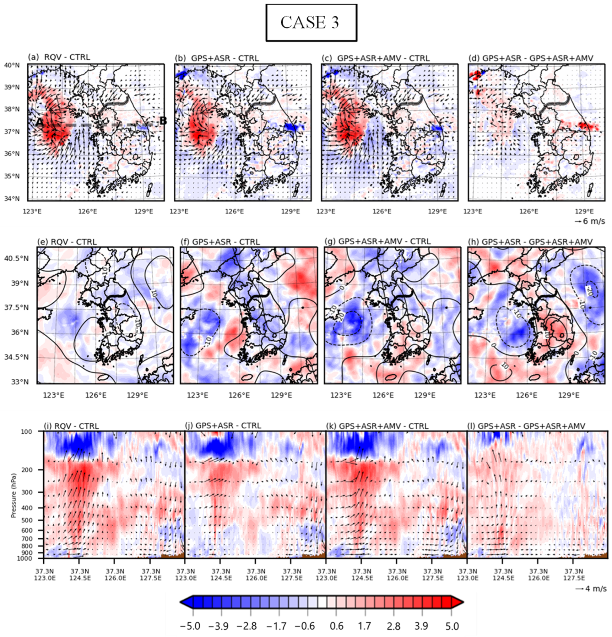
In Case 3, the BT observation reveals that the MCS approached from the north of the Yellow Sea toward the Korean Peninsula during the Changma front and shows the convective elements in the precipitation area (on the border of Gyeonggi and Gangwon Province) (Figure 4c). From Figure 6, it can be inferred that RQV, GPS + ASR, and GPS + ASR + AMV produced positive water vapor mixing ratios of approximately 5 g kg−1 and 0.8 g kg−1 over the MCS and precipitation area, respectively, compared to CTRL (Figure 6a–c). However, the coverage of the positive water vapor analysis increment area (5 g kg−1) in GPS + ASR was observed to be smaller than that of RQV (Figure 6a,b). Meanwhile, GPS + ASR + AMV increased the water vapor over the MCS area by 0.5 g kg−1 when compared to GPS + ASR (Figure 6d). The positive water vapor mixing ratio increments in RQV, GPS + ASR, and GPS + ASR + AMV were associated with the wind convergence at approximately 6 m s−1, 3 m s−1, and 5 m s−1, respectively (Figure 6a–c). This result is interrelated with the intensified low perturbation pressure over the MCS area in RQV, GPS + ASR, and GPS + ASR + AMV, with slightly different magnitudes and distributions (Figure 6e–g). RQV produced stronger increments of low pressure than GPS + ASR and GPS + ASR + AMV over 37.8°N 124.3°E at approximately 5 hPa (Figure 6e), while the other areas increased by approximately 3 hPa (Figure 6f,g). Such an increment caused stronger wind convergence. GPS + ASR increased the low perturbation pressure by approximately 2.5 hPa over most of the MCS area (Figure 6f), while GPS + ASR + AMV clearly intensified at approximately 4.5 hPa (Figure 6g). This convergence mainly came from the Yellow Sea, which broughtmoist air; hence, there was an increased in the water vapor mixing ratio over the MCS area in GPS + ASR + AMV when compared to GPS + ASR (Figure 6d). In addition, GPS + ASR + AMV produced the strongest westerly trough, extending to the precipitation area and increasing the wind toward the precipitation area that brought moist air from the MCS (Figure 6h). This result may present a rainfall distribution with larger coverage in the precipitation area. RQV increased the perturbation temperature by approximately ≥4.5 K over the core of the MCS area (approximately 37.3°N–124.5°E), centered at 300–250 hPa, when compared to CTRL (Figure 6i). GPS + ASR exhibited a higher perturbation temperature than CTRL by approximately 3 K and an updraft by approximately 1 m s−1 over the MCS area centered at the 500–200 hPa level, with a clearly shallower warm core than RQV (Figure 6j). GPS + ASR + AMV increased the perturbation temperature more than GPS + ASR by approximately 3 K and 0.5 K at the 800–500 hPa and 500–200 hPa levels, respectively (Figure 6k,l). These results were also associated with an increase in the updraft of approximately 3 m s−1, indicating that GPS + ASR + AMV produced a stronger convection of the MCS than GPS + ASR (Figure 6l).
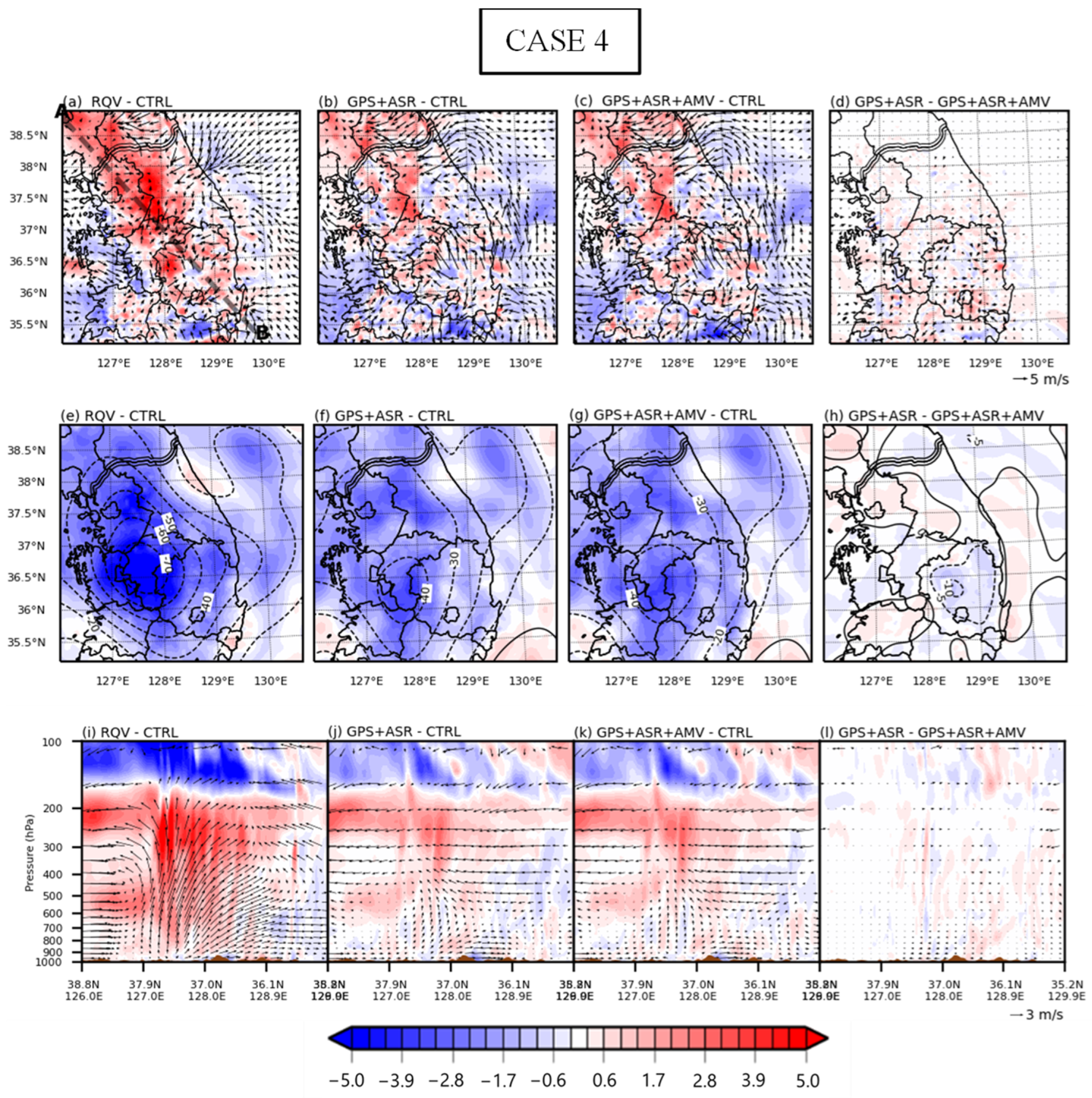
In Case 4, the satellite water vapor image shows a convective band centered between Gyeonggi and Gangwon Provinces (approximately 37.5°N–128°E) denoted by BT < 220 K (Figure 4d). From Figure 7, it can be inferred that RQV produced a larger coverage of water vapor content of approximately 5 g kg−1 when compared with the CTRL experiment (Figure 7a). Such an increment may produce a strong convective band. GPS + ASR increased the water vapor mixing ratio centered between Gyeonggi and Gangwon Provinces which was much closer to the BT observations (Figure 7b). GPS + ASR and GPS + ASR + AMV have similar water vapor contents, as indicated by small differences (Figure 7c,d). RQV, GPS + ASR, and GPS + ASR + AMV clearly increased the low perturbation pressures over the precipitation area by approximately 5, 3, and 3 hPa, respectively (Figure 7e–g), thus intensifying the wind convergence around the precipitation area by approximately 5 m s−1 (Figure 7a–c). In addition, RQV produced a much larger coverage of low perturbation pressure (Figure 7e), immensely strengthening the wind convergence (Figure 7a) when compared to GPS + ASR and GPS + ASR + AMV. GPS + ASR and GPS + ASR + AMV produced similar distributions of low perturbation pressure and wind convergence (Figure 7f,g) except that the increment of low perturbation pressure in GPS + ASR + AMV is higher by approximately 0.5 hPa over 36.2°N 128.5°E, inducing the northwesterly trough toward the convective area (Figure 7h). This result promoted stronger wind (0.5 m s−1) from the southwest, which slightly enhanced the wind convergence over the precipitation area in GPS + ASR + AMV (Figure 7d). The increased water vapor and wind convergence in RQV caused a strong updraft which accelerated the condensation of water vapor, creating a deep, warm core on the upper level of approximately 5 K, centered at 300 hPa (Figure 7i). These results suggest the development of deep convection. GPS + ASR also produced a deep, warm core at the upper level but at a smaller scale and at a lower magnitude of only 3 K (Figure 7j). GPS + ASR + AMV showed similarity to GPS + ASR (Figure 7j,k) except for the warm core in GPS + ASR + AMV, which was slightly stronger by 0.5 K at approximately 37.0°N–128.0°E (Figure 7l).
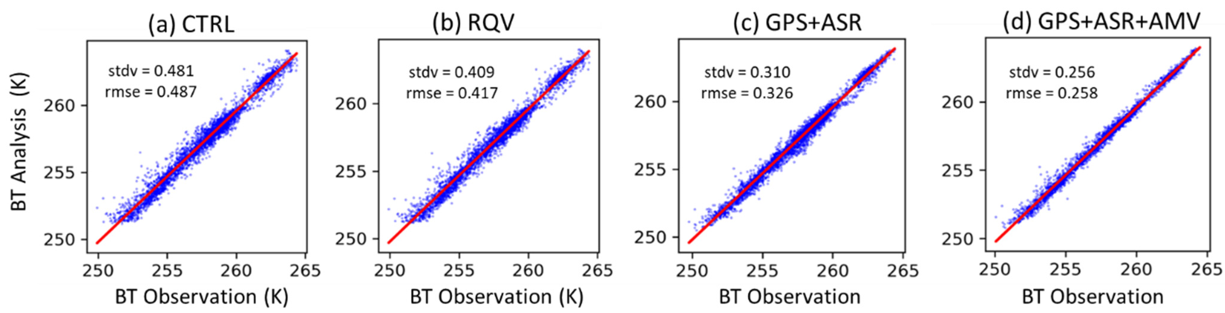
Figure 8 displays the scatter plots of the BT observations and the CRTM-simulated BT values at channel 10. Channel 10 was chosen for this analysis because this channel is more sensitive to clouds than any other water vapor channels (channel 8–10) [49]. The BT analysis for each simulation was simulated by CRTM using the pressure, temperature, water vapor, and water content of six hydrometeor types (rain, snow, ice, graupel, and hail) as input for the analysis model. Compared to CTRL, RQV reduced the standard deviation (STDV) and RMSE to 0.409 (by almost 15%) and 0.417 (by almost 14%). Meanwhile, GPS + ASR + AMV clearly simulated BT values closer to the observational values than other simulations, with reductions in the STDV to 0.256 (by almost 46%) and in the RMSE to 0.258 (by almost 47%). Further, the improvement of the BT in GPS + ASR + AMV was greatly superior to the BT in GPS + ASR (by almost 17% in the STDV and 20% in the RMSE). Such an improvement explains that the assimilation of AMVs also improved the pressure and temperature in GPS + ASR + AMV due to the link between the mass field and dynamic changes from AMV winds, leading to significant changes in the rainfall forecasts.

4.2. Analysis of Water Vapor and Dynamical Processes

To better understand the water vapor distribution and dynamics after using the modified variables in the initial fields, several kinds of weather charts are displayed for each simulation. Moisture convergence and flux represent the moisture process associated with precipitation. This study derived the water vapor convergence ( · q U ) and water vapor flux ( q U ) , which indicate that the magnitude and direction of the water vapor maintains rainfall, while the vertical velocity depicts vertical motion. A positive vertical velocity denotes a rising motion associated with precipitation. Figure 9 and Figure 10 show the water vapor convergence (g kg−1 s−1) overlaid by the water vapor flux (g kg−1 m s−1) vectors at 850 hPa and the vertical velocity (hPa h−1) overlaid by the wind (m s−1) at 700 hPa.
In Case 1, at 850 hPa, converging water vapor in the eastern region of the Yellow Sea and water vapor flux toward the precipitation area (Chungcheongnam and Gyeonggi Provinces) were generated in all experiments (Figure 9a–d). CTRL slightly captured water vapor convergence (60 × 10−6 g kg−1 s−1) in the eastern region of the Yellow Sea and flux (325 g kg−1 m s−1) toward the precipitation area (Figure 9a). RQV showed stronger and wider coverage of the water vapor convergence (90 × 10−6 g kg−1 s−1) in the Yellow Sea and flux (480 g kg−1 m s−1) toward the precipitation area than in other simulations (Figure 9b). This was mainly caused by the excessive water vapor in the initial field, as mentioned above (Figure 5a). GPS + ASR exhibited moisture convergence (75 g kg−1 m s−1) in the Yellow Sea and flux (450 g kg−1 m s−1) toward the precipitation area at a lower intensity and narrower scale than RQV (Figure 9c). Lastly, GPS + ASR + AMV evidently intensified the water vapor convergence to a greater extent than GPS + ASR by approximately 90 × 10−6 g kg−1 s−1, but the coverage was smaller than RQV (Figure 9d). The water vapor flux in GPS + ASR + AMV was of a similar magnitude to GPS + ASR at approximately 450 g kg−1 m s−1, but the coverage in GPS + ASR + AMV was smaller than GPS + ASR (Figure 9c,d). These results suggest that GPS + ASR + AMV had the optimal amount of moisture convergence and flux, leading to the accuracy of the rainfall prediction in terms of intensity and coverage. At 700 hPa, CTRL exhibited a lower vertical velocity by approximately 50 hPa h−1 when compared to the other simulations over the convergence area (east of the Yellow Sea) (Figure 10a). RQV, GPS + ASR, and GPS + ASR + AMV enhanced the strong vertical velocity above −75 hPa h−1 over the eastern region of the Yellow Sea, as expected with the enhancement of the convergence at 850 hPa (Figure 10b–d). However, RQV produced a strong vertical velocity (≥−75 hPa h−1) at a larger scale than GPS + ASR and GPS + ASR + AMV, extending to Chungcheongnam Province (Figure 10b–d). Over the inland Republic of Korea (near the northern region of Gyeonggi Area), only GPS + ASR + AMV exhibited a vertical velocity at approximately −65 hPa h−1, suggesting that only GPS + ASR + AMV may be capable of capturing significant rainfall over the northern part of the Gyeonggi Area (Figure 10d).
In Case 2, at 850 hPa, CTRL was unable to generate the convergence over the convective area as there was no wind convergence enhancement (Figure 9e), while water vapor convergence (90 × 10−6 g kg−1 s−1) and flux (280 g kg−1 m s−1) over the main convective area (approximately 36.6°N–124°E) were evidently observed in RQV, GPS + ASR, and GPS + ASR + AMV, with the largest scale observed in GPS + ASR + AMV (Figure 9f–h). GPS + ASR and GPS + ASR + AMV also showed convergence over the other convective area (36°N–122°E) (Figure 9g,h). In addition, over the inland Gyeonggi and Gangwon Provinces (the precipitation area), the magnitude of the water vapor flux in RQV was higher by approximately 100 g kg−1 m s−1 when compared to other simulations (Figure 9f). This result suggests that RQV may produce intense rainfall at the earlier hours of the forecast. Moreover, the direction of the water vapor flux in RQV was slightly turned northeast, which does not enhance the propagated west–east direction of the Changma front (Figure 9f). At 700 hPa, it can be inferred that CTRL exhibited almost zero vertical velocity when compared to other simulations over the convective area (approximately 36.6°N–124°E) (Figure 10e), which was associated with zero convergence at 850 hPa (Figure 9e). RQV, GPS + ASR, and GPS + ASR + AMV generated a vertical velocity of approximately ≥−60 hPa h−1 in the convective area (36.6°N–124°E) (Figure 10f–h), as expected with strong convergence at 850 hPa (Figure 9e–h). Moreover, GPS + ASR and GPS + ASR + AMV produced vertical velocities of 40 hPa h−1 and 45 hPa h−1, respectively, at 36°N–122°E (Figure 10g,h). This result suggests that GPS + ASR + AMV enhanced the development of the convective system along the Changma front (Figure 10h).
In Case 3, at 850 hPa, water vapor convergence was evidently seen over the MCS and precipitation area in all experiments (Figure 9i–l). However, only RQV, GPS + ASR, and GPS + ASR + AMV were able to intensify the water vapor convergence by approximately 90 × 10−6 g kg−1 s−1 at the center of the MCS (Figure 9j–l). Due to the increased water vapor convergence, the moisture flux was also increased by approximately 350 g kg−1 m s−1 (Figure 9j–l). Over the precipitation area, the water vapor convergence and flux were also intensified in RQV, GPS + ASR, and GPS + ASR + AMV, with differences in scale or magnitude (Figure 9j–l). RQV mainly generated water vapor convergence (≥75 × 10−6 g kg−1 s−1) that extended more toward Gangwon Province or on a larger scale than in GPS + ASR or GPS + ASR + AMV (Figure 9j). Meanwhile, GPS + ASR and GPS + ASR + AMV mainly produced water vapor convergence (≤75 × 10−6 g kg−1 s−1) in the precipitation area, but the coverage of water vapor convergence in GPS + ASR + AMV was larger than the coverage of water vapor convergence in GPS + ASR (Figure 9k,l). The water vapor flux toward the precipitation area in RQV was also larger by approximately 270 g kg−1 m s−1 (Figure 9j). Meanwhile, GPS + ASR and GPS + ASR + AMV produced water vapor flux values of approximately 230 g kg−1 m s−1 and 250 g kg−1 m s−1, respectively (Figure 9k,l). At 700 hPa, it can be observed that CTRL exhibited a very weak vertical velocity when compared to other simulations in the MCS and precipitation area (Figure 10i) and an associated weak enhancement of convergence at 850 hPa (Figure 9i). RQV, GPS + ASR, and GPS + ASR + AMV generated strong vertical velocities greater than 75 hPa h−1 in the MCS area (Figure 10j–l), as expected with the convergence enhancement at 850 hPa (Figure 9j–l). However, GPS + ASR mainly simulated a strong vertical velocity at a smaller scale than RQV and GPS + ASR + AMV (Figure 10k). Over the precipitation area, RQV, GPS + ASR, and GPS + ASR + AMV exhibited vertical velocities ≥−75 hPa h−1 (Figure 10j–l), but RQV had a larger scale than the other simulations (Figure 10j). In addition, GPS + ASR + AMV mainly produced a vertical velocity (≤−75 hPa h−1) over an increased coverage of the precipitation area than RQV or GPS + ASR (Figure 10l).
In Case 4, at 850 hPa, it can be inferred that CTRL generated a weak water vapor convergence and flux over the precipitation area (the northeastern part of of Chungcheongbuk Province) (Figure 9m). These results imply CTRL may not produce any precipitation. RQV showed the strongest water vapor convergence of approximately 90 × 10−6 g kg−1 s−1 over the precipitation area, which was associated with a water vapor flux of approximately 150 g kg−1 m s−1; this may result in the overestimation of rainfall (Figure 9n). GPS + ASR produced a weaker water vapor convergence (75 × 10−6 g kg−1 s−1) and flux (125 g kg−1 m s−1) compared to RQV (Figure 9o). GPS + ASR + AMV was similar to GPS + ASR, but the water vapor convergence was slightly intensified over the precipitation area by approximately 85 × 10−6 g kg−1 s−1 (Figure 9p). At 700 hPa, it can be observed that CTRL exhibited very weak vertical velocities when compared to other simulations in the precipitation area (Figure 10m), associated with a weak convergence at 850 hPa (Figure 9m). RQV generated the strongest vertical velocity of approximately 57 hPa h−1 (with a maximum of 70 hPa h−1) in the precipitation area (Figure 10n), as expected with strong convergence at the lower level (Figure 9n). GPS + ASR and GPS + ASR + AMV produced vertical velocities of approximately 32 and 37 hPa h−1, suggesting that GPS + ASR + AMV enhanced the development of the convective band more when compared to GPS + ASR, thus increasing the accuracy in predicting the maximum precipitation.

4.3. Qualitative Forecast Evaluation

The distribution of cumulative rainfall forecasts from each simulation were displayed with the AWS observation data. Figure 11 shows the cumulative rainfall generated by CTRL, RQV, GPS + ASR, and GPS + ASR + AMV for the forecast periods of Cases 1, 2, 3, and 4, respectively. For Case 1, the AWS observation showed an intense northeast-shifted rainband and two maximum precipitation areas marked by A and B, with the maximum precipitation reaching 120 mm (Figure 11a). CTRL predicted a small amount of precipitation and missed the intense rainfall over locations A and B (Figure 11b). CTRL assimilated no moisture information, causing no water to precipitate out of the air that would occur as rain. Meanwhile, RQV simulated a stronger and broader northeast-shifted rainband with the maximum precipitation reaching 200 mm over location A, but it did not predict any rainfall over location B (Figure 11c). GPS + ASR overpredicted rainfall of approximately 30 mm in the northeast-shifted rainband when compared to AWS, but it slightly improved the intense rainfall over location B by approximately 30 mm when compared to RQV (Figure 11d). The last experiment, GPS + ASR + AMV, captured a northeast-shifted rainband similar to the band in GPS + ASR, but it reduced the overestimation in some areas along the band (Figure 11e). Additionally, GPS + ASR + AMV captured a maximum precipitation of approximately 110 mm in location B that was similar to the AWS observations (Figure 11e).

4.4. Model Verification

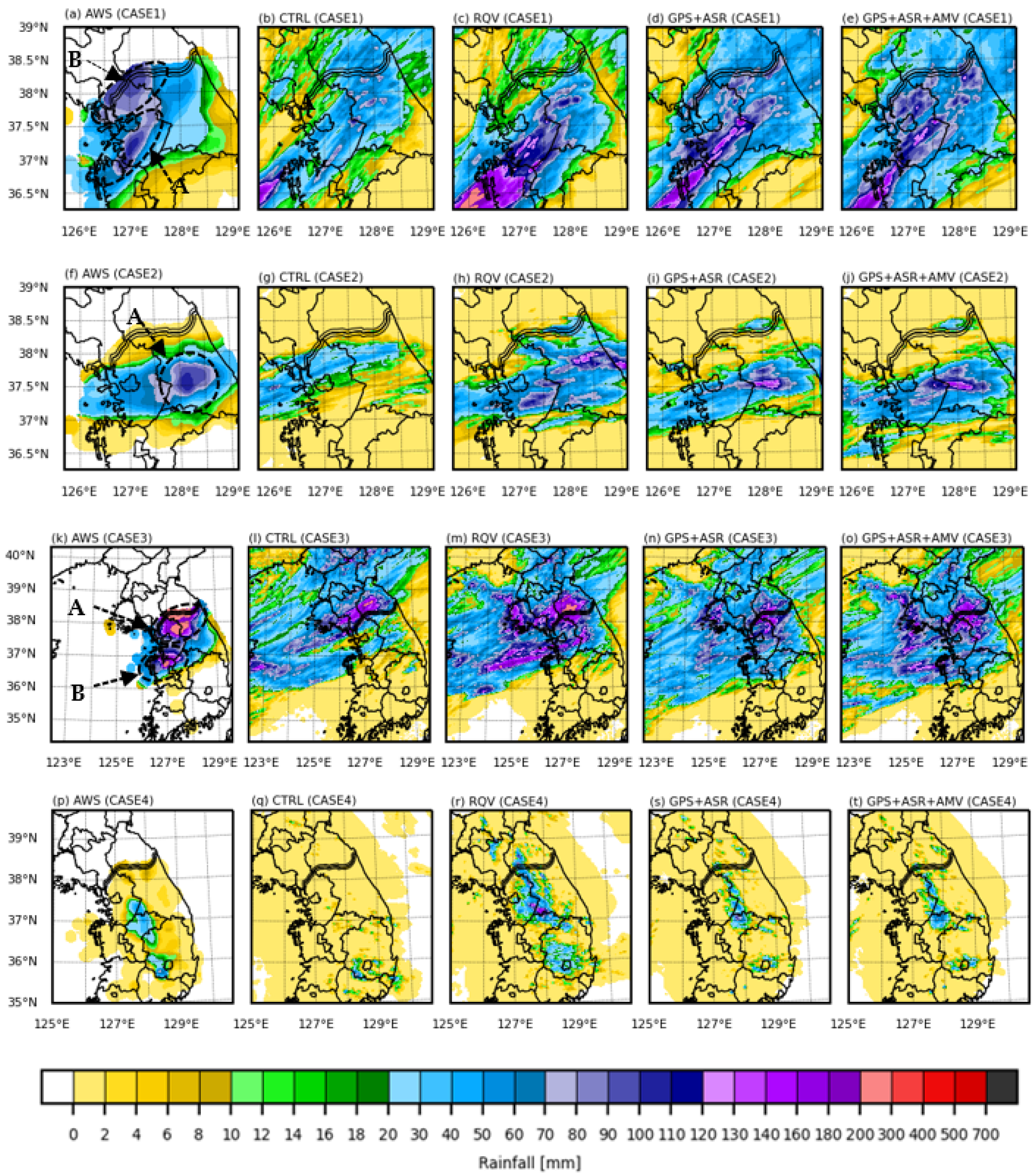
For Case 2, AWS observed an east-shifted rainband with a maximum precipitation reaching 120 mm over location A (Figure 11f). CTRL captured a weak and broken east-shifted rainband and missed the intense rainfall over location A (Figure 11g). Meanwhile, RQV generated the east-shifted precipitation well, but RQV missed the intense rainfall in location A and generated false alarms in the north and southwest of location A (Figure 11h). GPS + ASR generated the east-shifted rainband and the maximum precipitation of location A (Figure 11i). However, the east-shifted rainfall was narrower compared to the AWS observation, causing underprediction in some areas (Figure 11i). In addition, the maximum precipitation in GPS + ASR exceeded 120 mm, which was evidently overestimated when compared to AWS (Figure 11i). Meanwhile, GPS + ASR + AMV simulated the east-shifted rainfall well and more broadly than GPS + ASR while capturing the maximum precipitation of the location A; however, the intensity of the maximum precipitation overestimated the AWS (≥120 mm) (Figure 11j). Overall, GPS + ASR + AMV achieved the closest results to the AWS observation when compared to the other simulations.
For Case 3, the AWS mainly observed intense rainfall which exceeded 200 mm over locations A and B (Figure 11k). Evidently, CTRL did not generate rainfall for both locations A and B (Figure 11l). RQV generated rainfall over location A with a maximum precipitation of 200 mm (Figure 11m). However, the rainband was centered further north, causing the scale of rainfall on location A to be smaller than the AWS observations (Figure 11m). RQV also generated rainfall further north of location B (Figure 11m). Contrarily, GPS + ASR generated the rainfall centered slightly further south compared to RQV, which covered the rainfall area of location A better than RQV (Figure 11n). However, GPS + ASR underpredicted the intensity of the rainfall over location A (≥200 mm) (Figure 11n). For location B, GPS + ASR captured a slight rainfall of approximately 70 mm and clearly underestimated the AWS observations, though it reduced the underprediction by approximately 30 mm compared to the prediction of RQV (Figure 11n). Meanwhile, GPS + ASR + AMV showed a larger scale of rainfall with a higher intensity (exceeded 200 mm) in location A than the other simulations, showing better agreement with the AWS observations (Figure 11o). Moreover, GPS + ASR + AMV also captured rainfall events with intensities of ≥70 mm over location B; this is a higher intensity than other simulations and is closer to the AWS observations (Figure 11o).
A convective band occurred in Case 4 which caused rainfall in Chungcheongbuk Province and in some parts of Gyeongsangbuk Province, as observed by AWS, with a maximum precipitation of 70 mm (Figure 11p). Evidently, CTRL missed the main convective band rainfall in Chungcheongbuk Province and overestimated the small precipitation (±30 mm) in Gyeongsangbuk Province (Figure 11q). Meanwhile, RQV simulated a strong precipitation band (exceeded 120 mm), but the rainband was further north of Chungcheongbuk Province (Figure 11r). This strong rainband caused overpredictions in some areas of Gangwon Province and missed the rainfall in some areas of Chungcheongbuk Province (Figure 11r). The overestimation in Gyeongsangbuk Province also remained in RQV with larger coverage than in CTRL (Figure 11r). GPS + ASR captured the rainband further south of Chungcheongbuk Province when compared to RQV (Figure 11s). The intensity of the rainfall in GPS + ASR was mainly 70 mm (with the maximum exceeding 70 mm), and it was slightly overestimated when compared to AWS (Figure 11s). GPS + ASR + AMV also generated a precipitation similar to GPS + ASR, which may have been caused by the inclusion of AMV into the assimilation. which did not significantly influence the convective band case (Figure 11t). However, the rainfall distribution in GPS + ASR + AMV was slightly larger than in GPS + ASR, with the maximum precipitation only reaching 70 mm, which is closer to the AWS observations (Figure 11t).

4.5. Quantitative Forecast Evaluation

A quantitative verification was performed on the hourly rainfall to evaluate the forecast leading time. 
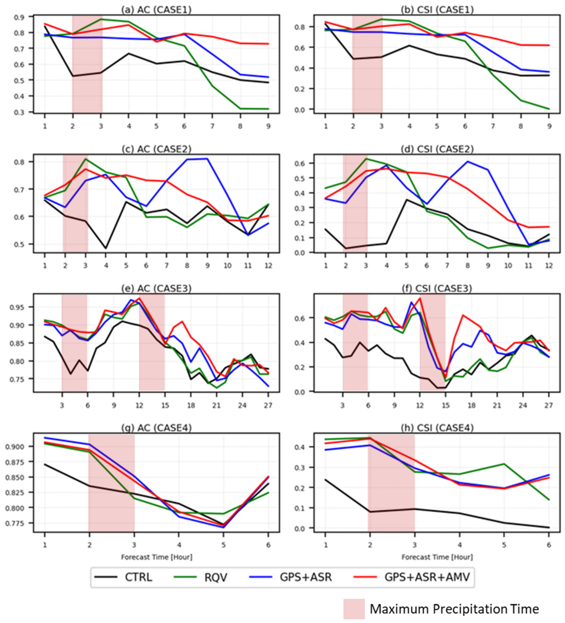
Figure 12 shows the categorical rainfall ≤ 0.1 mm (AC and CSI) using the forecast models and the AWS data of every 1 h forecast for Cases 1, 2, 3, and 4, respectively. The influence distance of the AWS in Republic of Korea was effectively 10 km × 10 km. Thus, the precipitation from the models of domain 3 averaged nine grid points when compared to the AWS.
For Case 1 (Figure 12a,b), due to the underprediction of rainfall, CTRL showed the lowest AC and CSI scores in terms of rainfall classification because CTRL missed the rainfall for all the forecast times. RQV increased the AC and CSI scores by approximately 45% only during the first 6 h compared to CTRL and had the worst AC and CSI scores relative to the other experiments. Both the AC and CSI scores of GPS + ASR also showed an increase (of approximately 35%) when compared to CTRL until the sixth hour, but at later hours, both scores were reduced. GPS + ASR + AMV increased the scores less than RQV during the first 5 h because rainfall classification only determines precipitation larger than 0.1 mm but does not determine the extent of overestimation. Overall, at most forecast times, GPS + ASR + AMV showed higher AC and CSI scores than other experiments, especially near the forecast completion.
For Case 2 (Figure 12c,d), the RQV experiment increased the AC and CSI scores by approximately 40% when compared to CTRL until the fifth hour before continuing to decrease and achieving a lower score compared to CTRL. GPS + ASR improved the AC and CSI scores by approximately 60% over time than CTR except at the sixth hour because there many false alarms occurred, while GPS + ASR + AMV increased the scores by approximately 65% during the first 9 h and by 20% after 9 h.
For Case 3 (Figure 12e,f), due to the underestimation, CTRL’s AC and CSI scores were very low due to the missed rainfall. The RQV experiment showed an improvement in the AC and CSI scores of approximately 40% during the first 15 h, but the scores continued to decrease after the 15th hour. The improvements in the AC and CSI scores in GPS + ASR were not higher than RQV, but the improvement of GPS + ASR persisted for a longer period. GPS + ASR + AMV improved by roughly 18% when compared to GPS + ASR at most forecast times except at approximately the 12–15th hours due to the prediction of more false alarms when compared to GPS + ASR during these hours. In general, GPS + ASR + AMV increased the statistics’ scores for longer forecast times than other simulations.
For Case 4 (Figure 12g,h), CTRL produced the lowest AC and CSI scores for most of the forecast times. RQV improved the AC score by ±10% when compared to CTRL during the first 2 h before decreasing. RQV mostly increased the CSI score by ±60% when compared to CTRL, except for the third and sixth hours. Considering the AC score, GPS + ASR and GPS + ASR + AMV increased the score by 5% and 7% when compared to CTRL during the first 3 h, respectively. Considering the CSI score, GPS + ASR and GPS + ASR + AMV increased the score by 50% and 58% when compared to CTRL throughout the forecast times, respectively. Overall, the best improvements were observed in GPS + ASR + AMV.
The cumulative rainfall forecasts were also verified with AWS observation data through quantitative error (RMSE and BIAS), the classification of rainfall occurrences (>0.1) (accuracy and CSI), and the pattern correlation method. Table 3 shows the quantitative verification of the cumulative rainfall for Cases 1, 2, 3, and 4, as well as the average of all cases. For Case 1 (Table 3), RQV increased the RMSE by approximately 35% compared to CTRL. This error was mainly caused by overestimation, as indicated by a BIAS value of 20.17 mm. Meanwhile, GPS + ASR showed a decrease in the RMSE by approximately 3% when compared to CTRL, with the BIAS of 9.5 mm indicating a decrease in overestimation by approximately 52% compared to RQV. GPS + ASR + AMV decreased the RMSE more, by approximately 12% when compared to CTRL, and the BIAS error was decreased by approximately 55% when compared to RQV. Considering the category classifications, the scores of all experiments were mostly comparable to CTRL. However, the best performances were achieved by GPS + ASR + AMV, with an increased score of 2% for AC and CSI when compared to CTRL. Pattern correlation indicates that RQV had the worst correlation due to the excessive overestimation, making it less correlated to the AWS observations. Meanwhile, GPS + ASR + AMV produced the best correlation, with an increase of approximately 50% compared to that of CTRL, because it captured the two locations of maximum rainfall.
For Case 2 (Table 3), compared to CTRL, all experiments showed a reduction in the RMSE or BIAS error. RQV, GPS + ASR, and GPS + ASR + AMV decreased the RMSE by approximately 32%, 45%, and 46% respectively. RQV showed a 72% reduction of BIAS, though the BIAS value of 3.44 mm indicates overestimation. Moreover, GPS + ASR and GPS + ASR + AMV decreased the BIAS error by approximately 90% and 95%, respectively. However, GPS + ASR slightly underestimated (−1.7 mm), while GPS + ASR + AMV slightly overestimated (0.55 mm). The AC and CSI scores also exhibited an improvement in all experiments compared to that of CTRL. GPS + ASR and GPS + ASR + AMV produced the best performances, with AC and CSI score improvements of 11% and 20%, respectively. This could primarily be attributed to the correction of the maximum precipitation location. PC shows an increased correlation for all experiments when compared to CTRL. RQV, GPS + ASR and GPS + ASR + AMV produced comparable correlations with 71%, 74%, and 74.5% improvements, respectively.
For Case 3 (Table 3), RQV, GPS + ASR, and GPS + ASR + AMV reduced the RMSE values by approximately 30%, 34%, and 38%, respectively. Additionally, the BIAS error indicates that RQV, GPS + ASR, and GPS + ASR + AMV reduced the underestimation by approximately 57%, 87%, and 89%, respectively. Considering the rainfall occurrences, the AC and CSI scores possess comparable values between the assimilation experiments. RQV, GPS + ASR, and GPS + ASR + AMV produced approximately 0.9%, 2.2%, and 4.4% improvements in the AC score, and improvements of approximately 0.24%, 4.35%, and 3.74% in the CSI score when compared to CTRL. The PC score reveals that GPS + ASR + AMV produced the best score, with an increased value of 60% compared to CTRL. Meanwhile, RQV and GPS + ASR increased by approximately 49% and 56%, respectively.
Considering Case 4 (Table 3), RQV produced a reduction of only roughly 0.18% in the RMSE when compared to CTRL. Additionally, RQV generated a BIAS of 2.18 mm, indicating an overestimation. GPS + ASR and GPS + ASR + AMV show comparable reductions of 18% and 19% for RMSE and 22% and 34% for the BIAS error. GPS + ASR and GPS + ASR + AMV generated similar AC and CSI scores. Both improved the AC and CSI scores by 22% and 86%, respectively, compared to those of CTRL. RQV, GPS + ASR, and GPS + ASR + AMV improved the PC values by 82%, 88%, and 96% when correlated to AWS observations.
From the average of the quantitative verification of all cases (Table 3), the lowest RMSE and BIAS error were achieved by GPS + ASR + AMV, followed by the GPS + ASR RQV, and CTRL experiments. The values of the reduction percentages of the RMSE and BIAS error in GPS + ASR + AMV reached 31% and 80% compared to CTRL. On a categorical quantitative score, GPS + ASR + AMV performed the best, with AC and CSI increases of 10% and 16%, respectively. The PC also established that GPS + ASR + AMV was the most correlated to the AWS by approximately 71%.
To further investigate the impact of the assimilation experiments on rainfall forecasts, the ETS was calculated using the simulation forecast fields and the AWS observations as the function of the rainfall threshold per hour (mm) (Figure 13). Four rainfall thresholds, light rain (0.1 ≤ R ≤ 3), moderate rain (3 ≤ R ≤ 15), heavy rain (15 ≤ R ≤ 30), and very heavy rain (R ≥ 30), were used. The ETSs of the four cases were averaged. Compared to CTRL, RQV, GPS + ASR, and GPS + ASR + AMV improved the ETS by 38%, 50%, and 59% for the light rain, respectively. For moderate rain, GPS + ASR + AMV showed the highest accuracy with a 62% improvement in the ETS compared to that of CTRL; however, RQV and GPS + ASR only produced improvements of 28% and 44%, respectively. RQV, GPS + ASR, and GPS + ASR + AMV increased the heavy rain ETS by approximately 28%, 63%, and 53%, respectively. For the very heavy rain threshold, the ETS showed a small value because the occurrence of very heavy rainfall was rare. The enhancement by the assimilation experiments was also small, and RQV, GPS + ASR, and GPS + ASR + AMV produced similar 23% increases in the ETS compared to that of CTRL. Overall, it can be inferred that the improvement in experiment assimilations primarily corresponded to light and moderate rain, with GPS + ASR + AMV showing the best improvement.

4.6. Comparison of Forecast Variables Fields

The vertical profile of the water vapor mixing ratio (g kg−1), temperature (°C), wind (m s−1), and geopotential height (m) were verified using radiosonde observations for each case. The time and location of verification were selected based on the available data and proximity to the precipitation area during the forecast period of each case. There were 12 radiosonde observations validated (Figure 3). The vertical biases were averaged using these 12 radiosonde observations.
For Q variables (Figure 14a), it was evident that the water vapor mixing ratio of CTRL underestimated the radiosonde observations at all levels. RQV reduced the underestimation in CTRL from 925 to 400 hPa and the overestimation from 925 to 600 hPa; however, the underestimation was reduced from 600 to 400 hPa. Above 400 hPa, RQV had increased the underestimation when compared to CTRL. This result showed that RQV was incapable of maintaining a high water vapor bias during the forecast, leading to frequent rainfall underestimations at the end of the forecast hours. GPS + ASR and GPS + ASR + AMV reduced the underestimation of the water vapor mixing ratio from CTRL at all levels without producing an overestimation as large as RQV from 925 to 600 hPa. A near-zero value of bias was mostly achieved by GPS + ASR + AMV at all levels. For T variables (Figure 14b), CTRL showed a warm bias below 400 hPa and above 300 hPa, but a cold bias was demonstrated between 400 and 300 hPa. All the experiments reduced the warm bias from 900 to 500 hPa and the cold bias from 400 to 300 hPa. GPS + ASR + AMV showed the most reduction in the BIAS when compared to CTRL. For wind variables (Figure 14c), CTRL produced a negative BIAS below 500 hPa and a positive BIAS above 500 hPa. At below 500 hPa, RQV, GPS + ASR, and GPS + ASR + AMV showed reductions in the negative BIAS of wind when compared to CTRL. Meanwhile, above 500 hPa, only GPS + ASR and GPS + ASR + AMV were capable of reducing the positive BIAS of wind. In general, a near-zero BIAS value was mostly produced by GPS + ASR + AMV. For geopotential height variables (Figure 14d), CTRL showed a positive BIAS value at all levels. RQV, GPS + ASR, and GPS + ASR + AMV reduced the positive BIAS of CTRL at all levels. However, GPS + ASR + AMV substantially showed the lowest BIAS at all levels when compared to the other simulations.

5. Conclusions

The performance of the 3DVAR assimilation with GPSRO refractivity, all-sky radiance, and AMV assimilation was investigated based on four heavy rainfall events during summertime in the Republic of Korea. Three cases included rainfall associated with the Changma front with different forecast periods, and one case included convective rainfall. These cases were selected because they facilitate a better understanding of the variation in impact of assimilation on the meso (short- and long-term periods) and convective scales.
To determine the contribution of each simulation in generating rainfall forecasts, the dynamical and thermodynamic increments in the initial field were analyzed. It was observed that all simulations were able to increase the water vapor content for the extreme rainfall associated with the Changma front and convective cases. However, the estimation of water vapor from the in-cloud humidity radar reflectivity in the RQV simulation exhibited extra and spurious water vapor content, overestimating the rainfall during the first 4 h. The GPSRO refractivity mainly corrected the moisture at a low-troposphere level associated with a warmer condition, triggering the enhancement of the evaporation rate. However, in this study, most cases (e.g., Cases 2, 3, and 4) had limited GPSRO refractivity observations around the rainfall systems; thus, the all-sky radiance data played major roles in providing the water vapor. GPS + ASR and GPS + ASR + AMV assimilated the all-sky radiance data, which means both cloud-affected and clear-air radiances were included. The cloud-affected radiances enhanced the water vapor and temperature structures of the cloud systems at the low- to mid-atmospheric layers. This modification was combined with the finer microphysical structure of clouds from radar in both GPS + ASR and GPS + ASR + AMV, which initialized a better structure and environment for the cloud precipitation analysis, contributing to the more accurate rainfall forecasts. The clear-air radiances also played significant roles by providing data outside the precipitation areas and prior to the formation of storm fields, initializing mass and thermal state information in larger areas which increased the long-range forecast accuracy. The additional AMVs in GPS + ASR + AMV drove significant changes in synoptic- and meso-winds, interrelating them with the pressure fields. These changes in winds were associated with enhanced wind convergence and low pressure at the lower level. Due to the adjustment of the water vapor mixing ratio and wind convergence at a low level, the intensity and acceleration of the water vapor condensation in GPS + ASR + AMV were increased, resulting in deep warming increments because of latent heat released from the condensation. This acceleration contributed to the accuracy of predicting the timing and intensity of heavy rainfall. The analysis of the observed and simulated BT values also demonstrates that GPS + ASR + AMV produced significant reductions in error statistics in the CRTM BT simulation, implying that the input of the model variables (pressure, temperature, water vapor, hydrometeors) to CRTM model was the most accurate, and the inclusion of the AMV winds corresponded with pressure and temperature through the mass field and dynamic linkage. Further, from the weather analysis, the assimilation of the AMV data changed the intensity and dynamical water vapor convergence and flux, which resulted in a more sustained heavy rainfall with an increasing lead time. However, the assimilation of AMVs had a minor impact on convective-scale storm rainfall. This is mainly because the AMV data has passed through strict quality control measures which reduced the amount of data, using only for synoptic and mesoscale data coverage.
In summary, the qualitative and quantitative cumulative rainfall verifications reveal that GPS + ASR + AMV had a better agreement for both rainfall and intensity compared to other simulations for the meso- and convective-scales. The error reduction can be as great as 31% for the RMSE and 80% for the BIAS, while the improvement in the skill scores can be up to 10% for AC, 16% for CSI, and 53% for PC compared to CTRL. In particular, the ETS indicates that GPS + ASR + AMV has the best ability to predict light and moderate rainfall. The calculation of the vertical profile bias against the radiosonde data shows that GPS + ASR + AMV demonstrated the greatest improvements in the water vapor mixing ratio, temperature, wind, and geopotential height fields when compared to the other simulations at most levels.
In this study, the 3DVAR technique was used for assimilation. However, 3DVAR is limited by issues, such as the use of static background error covariances, making it impractical for manifesting the flow-dependent feature of the atmosphere. The ensemble-based assimilation method is expected to provide flow-dependent background error covariances. Additionally, the adaptive observation error inflation (AOEI) method, which utilizes an ensemble-based data assimilation framework, is expected to enhance the assimilation of all-sky radiances [50]. In addition, only water vapor channels were used to assimilate the all-sky radiances. Assimilating other surface infrared channels will provide more benefits but will also pose various challenges and require a careful treatment of surface emissivity; thus, it is left for future research.

Author Contributions

M.I.H. wrote the original draft, assisted with data curation, and performed the formal analysis, investigation, software coding, and visualization of the research article. K.-H.M. conceptualized the paper, supervised and administered the project, performed the formal analysis, provided resources and funding, and reviewed and edited the paper. J.-W.L. provided the radar processing code and technical support. All authors have read and agreed to the published version of the manuscript.

Funding

This work is supported by the National Research Foundation of Korea (NRF) grant funded by the Korea government (MSIT) (No. 2021R1A4A1032646 and No. 2022R1A2C1012361).

Conflicts of Interest

The authors declare that they have no known competing financial interest or personal relationships that could have appeared to influence the work reported in this paper.

References

  1. Dance, S.L.; Ballard, S.P.; Bannister, R.N.; Clark, P.; Cloke, H.L.; Darlington, T.; Flack, D.L.A.; Gray, S.L.; Hawkness-Smith, L.; Husnoo, N.; et al. Improvements in Forecasting Intense Rainfall: Results from the FRANC (Forecasting Rainfall Exploiting New Data Assimilation Techniques and Novel Observations of Convection) Project. Atmosphere 2019, 10, 125. [Google Scholar] [CrossRef]
  2. Milan, M.; MacPherson, B.; Tubbs, R.; Dow, G.; Inverarity, G.; Mittermaier, M.; Halloran, G.; Kelly, G.; Li, D.; Maycock, A.; et al. Hourly 4D-Var in the Met Office UKV operational forecast model. Q. J. R. Meteorol. Soc. 2020, 146, 1281–1301. [Google Scholar] [CrossRef]
  3. Hawkness-Smith, L.; Simonin, D. Radar reflectivity assimilation using hourly cycling 4D-Var in the Met Office Unified Model. Q. J. R. Meteorol. Soc. 2021, 147, 1516–1538. [Google Scholar] [CrossRef]
  4. Min, K.; Choo, S.; Lee, D.; Lee, G. Evaluation of WRF Cloud Microphysics Schemes Using Radar Observations. Weather Forecast. 2015, 30, 1571–1589. [Google Scholar] [CrossRef]
  5. Xiao, Q.; Kuo, Y.-H.; Sun, J.; Lee, W.-C.; Lim, E.; Guo, Y.-R. Assimilation of Doppler radar observations with a regional 3DVAR system: Impact of Doppler velocities on forecasts of a heavy rainfall case. J. Appl. Meteorol. 2005, 44, 768–788. [Google Scholar] [CrossRef]
  6. Gao, J.; Stensrud, D.J. Assimilation of reflectivity data in a convective-scale, cycled 3DVAR framework with hydrometeor classification. J. Atmos. Sci. Res. 2012, 69, 1054–1065. [Google Scholar] [CrossRef]
  7. Wang, H.; Sun, J.; Fan, S.; Huang, X.-Y. Indirect assimilation of radar reflectivity with WRF 3D-Var and its impact on prediction of four summertime convective events. J. Appl. Meteorol. Climatol. 2013, 52, 889–902. [Google Scholar] [CrossRef]
  8. Lee, J.-W.; Min, K.-H.; Lee, Y.-H.; Lee, G. X-Net-Based Radar Data Assimilation Study over the Seoul Metropolitan Area. Remote Sens. 2020, 12, 893. [Google Scholar] [CrossRef]
  9. Lee, J.W.; Min, K.-H.; Lim, K.S. Comparing 3DVAR and hybrid radar data assimilation methods for heavy rain forecast. Atmos. Res. 2022, 270, 106062. [Google Scholar] [CrossRef]
  10. Gao, S.; Sun, J.; Min, J.; Zhang, Y.; Ying, Z. A Scheme to Assimilate “No Rain” Observations from Doppler Radar. Weather Forecast. 2018, 33, 71–88. [Google Scholar] [CrossRef]
  11. Pan, S.; Gao, J.; Stensrud, D.J.; Wang, X.; Jones, T.A. Assimilation of Radar Radial Velocity and Reflectivity, Satellite Cloud Water Path, and Total Precipitable Water for Convective-Scale NWP in OSSEs. J. Atmos. Ocean. Technol. 2018, 35, 60–89. [Google Scholar] [CrossRef]
  12. Yang, S.; Huang, Z.; Huang, C.; Tsai, C.; Yeh, T. A Case Study on the Impact of Ensemble Data Assimilation with GNSS-Zenith Total Delay and Radar Data on Heavy Rainfall Prediction. Mon. Weather Rev. 2020, 148, 1075–1098. [Google Scholar] [CrossRef]
  13. Kuo, Y.-H.; Sokolovskiy, S.; Anthes, R.; Andenberghe, F.V. Vandenberghe. Assimilation of GPS radio occultation data for numerical weather prediction. Terr. Atmos. Ocean. Sci. 2000, 11, 157–186. [Google Scholar] [CrossRef]
  14. Chen, S.; Kuo, Y.; Huang, C. The Impact of GPS RO Data on the Prediction of Tropical Cyclogenesis Using a Nonlocal Observation Operator: An Initial Assessment. Mon. Weather Rev. 2020, 148, 2701–2717. [Google Scholar] [CrossRef]
  15. Chang, C.C.; Yang, S.C. Impact of assimilating Formosat-7/COSMIC-II GNSS radio occultation data on heavy rainfall prediction in Taiwan. Terr. Atmos. Ocean. Sci. 2022, 33, 7. [Google Scholar] [CrossRef]
  16. Boyaj, A.; Dasari, H.P.; Rao, Y.V.R.; Ashok, K.; Hoteit, I. Assimilation of global positioning system radio occultation refractivity for the enhanced prediction of extreme rainfall events in southern India. Meteorolol. Appl. 2022, 29, e2103. [Google Scholar] [CrossRef]
  17. Cheng, W.; Xu, Y.; Deng, Z.; Gu, C. GPS Radio Occultation Data Assimilation in the AREM Regional Numerical Weather Prediction Model for Flood Forecasts. Adv. Meteorol. 2018, 2018, 1–9. [Google Scholar] [CrossRef]
  18. King, M.D.; Menzel, W.P.; Kaufman, Y.J.; Tanré, D.; Gao, B.-C.; Platnick, S.; Ackerman, S.A.; Remer, L.A.; Pincus, R.; Hubanks, P.A. Cloud and aerosol properties, precipitable water, and profiles of temperature and water vapor from MODIS. IEEE Trans. Geosci. Remote Sens. 2003, 41, 442–458. [Google Scholar] [CrossRef]
  19. Okamoto, K.; Sawada, Y.; Kunii, M. Comparison of assimilating all-sky and clear-sky infrared radiances from Himawari-8 in a mesoscale system. Q. J. R. Meteorol. Soc. 2019, 145, 745–766. [Google Scholar] [CrossRef]
  20. Xu, D.-M.; Liu, Z.-Q.; Fan, S.-Y.; Chen, M.; Shen, F.-F. Assimilating all-sky infrared radiances from Himawari-8 using the 3DVar method for the prediction of a severe storm over North China. Adv. Atmos. Sci. 2021, 38, 661–676. [Google Scholar] [CrossRef]
  21. Zhang, Y.; Stensrud, D.J.; Zhang, F. Simultaneous Assimilation of Radar and All-Sky Satellite Infrared Radiance Observations for Convection-Allowing Ensemble Analysis and Prediction of Severe Thunderstorms. Mon. Weather Rev. 2019, 147, 4389–4409. [Google Scholar] [CrossRef]
  22. Wang, J.; Zhang, L.; Guan, J.; Zhang, M. Evaluation of combined satellite and radar data assimilation with POD-4DEnVar method on rainfall forecast. Appl. Sci. 2020, 10, 5493. [Google Scholar] [CrossRef]
  23. Jones, T.A.; Skinner, P.; Yussouf, N.; Knopfmeier, K.; Reinhart, A.; Wang, X.; Bedka, K.; Smith, W., Jr.; Palikonda, R. Assimilation of GOES-16 Radiances and Retrievals into the Warn-on-Forecast System. Mon. Weather Rev. 2020, 148, 1829–1859. [Google Scholar] [CrossRef]
  24. Chen, K.; Guan, P. The Impacts of Assimilating Fengyun-4A Atmospheric Motion Vectors on Typhoon Forecasts. Atmosphere 2023, 14, 375. [Google Scholar] [CrossRef]
  25. Wu, T.-C.; Liu, H.; Majumdar, S.J.; Velden, C.S.; Anderson, J.L. Andersson. Influence of assimilating satellite derived atmospheric motion vector observations on numerical analyses and forecasts of tropical cyclone track and intensity. Mon. Weather Rev. 2014, 142, 49–71. [Google Scholar] [CrossRef]
  26. Zhao, J.; Gao, J.; Jones, T.A.; Hu, J. Impact of assimilating high-resolution Atmospheric Motion Vectors on convective scale short-term forecasts: 1. Observing system simulation experiment (OSSE). J. Adv. Model. Earth Syst. 2021, 13, e2021MS002484. [Google Scholar] [CrossRef]
  27. Kim, D.; Kim, H.M. Effect of Assimilating Himawari-8 Atmospheric Motion Vectors on Forecast Errors over East Asia. J. Atmos. Ocean. Technol. 2018, 35, 1737–1752. [Google Scholar] [CrossRef]
  28. Barker, D.M.; Huang, W.; Guo, Y.-R.; Bourgeois, A.J.; Xiao, Q.N. A three-dimensional variational data assimilation system for MM5: Implementation and initial results. Mon. Weather Rev. 2004, 132, 897–914. [Google Scholar] [CrossRef]
  29. Barker, D.M.; Huang, X.Y.; Liu, Z.; Auligne, T.; Zhang, X.; Rugg, S. The weather research and forecasting (WRF) model’s community variational/ensemble data assimilation system: WRFDA. Bull. Am. Meteorol. Soc. 2012, 93, 831–843. [Google Scholar] [CrossRef]
  30. Ide, K.; Courtier, P.; Ghil, M.; Lorenc, A.C. Unified notation for data assimilation: Operational, sequential and variational. J. Meteorol. Soc. Jpn. 1999, 75, 181–189. [Google Scholar] [CrossRef]
  31. Parrish, D.F.; Derber, J.C. The National Meteorological Center’s spectral statistical-interpolation analysis system. Mon. Weather Rev. 1992, 120, 1747–1763. [Google Scholar] [CrossRef]
  32. Han, Y.; Van Delst, P.; Liu, Q.; Weng, F.; Yan, B.; Han, Y. JCSDA Community Radiative Transfer Model (CRTM)-Version 1; NOAA Technical Report; NESDIS: Silver Spring, MD, USA, 2006. [Google Scholar]
  33. Dee, D.; Uppala, S.M. Variational bias correction of satellite radiance data in the ERA–Interim reanalysis. Q. J. R. Meteorol. Soc. 2009, 135, 1830–1841. [Google Scholar] [CrossRef]
  34. Liu, Z.; Schwartz, C.S.; Snyder, C.; Ha, S.-Y. Impact of assimilating AMSU-A radiances on forecasts of 2008 Atlantic tropical cyclones initialized with a limited-area Ensemble Kalman Filter. Mon. Weather Rev. 2012, 140, 4017–4034. [Google Scholar] [CrossRef]
  35. Zhu, Y.; Derber, J.; Collard, A.; Dee, D.; Treadon, R.; Gayno, G.; Jung, J.A. Enhanced radiance bias correction in the National Centers for Environmental Prediction’s Gridpoint Statistical Interpolation data assimilation system. Q. J. R. Meteorol. Soc. 2014, 140, 1479–1492. [Google Scholar] [CrossRef]
  36. Derber, J.C.; Wu, W.S. The use of TOVS cloud-cleared radiance in the NCEP SSI analysis system. Mon. Weather Rev. 1998, 126, 2287–2299. [Google Scholar] [CrossRef]
  37. Okamoto, K.; McNally, A.P.; Bell, W. Progress towards the assimilation of all-sky infrared radiances: An evaluation of cloud effects. Q. J. R. Meteorol. Soc. 2014, 140, 1603–1614. [Google Scholar] [CrossRef]
  38. Okamoto, K. Evaluation of IR radiance simulation for all-sky assimilation of Himawri-8/AHI in a mesoscale NWP system. Q. J. R. Meteorol. Soc. 2017, 143, 1517–1527. [Google Scholar] [CrossRef]
  39. Phinney, R.A.; Anderson, D.L. On the radio occultation method for studying planetary atmosphere. J. Geophys. Res. 1968, 73, 1819–1827. [Google Scholar] [CrossRef]
  40. Smith, E.K.; Weintraub, S. The constants in the equation for atmospheric refractivity index at radio frequencies. J. Res. Natl. Inst. Stand. Technol. 1953, 50, 39–41. [Google Scholar] [CrossRef]
  41. Ye, B.-Y.; Lee, G.; Park, H.-M. Identification and removal of non-meteorological echoes in dual-polarization radar data based on a fuzzy logic algorithm. Adv. Atmos. Sci. 2015, 32, 1217–1230. [Google Scholar] [CrossRef]
  42. Di, D.; Ai, Y.; Li, J.; Shi, W.; Lu, N. Geostationary satellite-based 6.7 μm band best water vapor information layer analysis over the Tibetan Plateau. J. Geophys. Res. Atmos. 2016, 121, 4600–4613. [Google Scholar] [CrossRef]
  43. Skamarock, W.C.; Klemp, J.B.; Dudhia, J.; Gill, D.O.; Barker, D.M.; Wang, W.; Powers, J.G. A Description of the Advanced Research WRF Version 2; National Center for Atmospheric Research Boulder Co Mesoscale and Microscale Meteorology Div.; Mesoscale and Microscale Meteorology Division, National Center for Atmospheric Research: Boulder, CA, USA, 2005. [Google Scholar]
  44. Kain, J.S.; Fritsch, J.M. Convective Parameterization for Mesoscale Models: The Kain-Fritsch Scheme. In The Representation of Cumulus Convection in Numerical Models. Meteorological Monographs; Emanuel, K.A., Raymond, D.J., Eds.; American Meteorological Society: Boston, MA, USA, 1993. [Google Scholar] [CrossRef]
  45. Lim, K.-S.S.; Hong, S.-Y. Development of an effective double-moment cloud microphysics scheme with prognostic cloud condensation nuclei (CCN) for weather and climate models. Mon. Weather Rev. 2010, 138, 1587–1612. [Google Scholar] [CrossRef]
  46. Tewari, M.; Chen, F.; Wang, W.; Dudhia, J.; LeMone, M.A.; Mitchell, K.; Cuenca, R.H. Implementation and verification of the unified NOAH land surface model in the WRF model. In Proceedings of the 20th Conference on Weather Analysis and Forecasting/16th Conference on Numerical Weather Prediction, Seattle, WA, USA, 12–16 January 2004; Volume 1115. [Google Scholar]
  47. Hong, S.Y.; Noh, Y.; Dudhia, J. A new vertical diffusion package with an explicit treatment of entrainment processes. Mon. Weather Rev. 2006, 134, 2318–2341. [Google Scholar] [CrossRef]
  48. Dudhia, J. Numerical study of convection observed during the winter monsoon experiment using a mesoscale two-dimensional model. J. Atmos. Sci. 1989, 46, 3077–3107. [Google Scholar] [CrossRef]
  49. Okamoto, K.; Hayashi, M.; Hashino, T.; Nakagawa, M.; Okuyama, A. Examination of all-sky infrared radiance simulation of Himawari-8 for global data assimilation and model verification. Q. J. R. Meteorol. Soc. 2021, 147, 3611–3627. [Google Scholar] [CrossRef]
  50. Minamide, M.; Zhang, F. Adaptive Observation Error Inflation for Assimilating All-Sky Satellite Radiance. Mon. Weather Rev. 2017, 145, 1063–1081. [Google Scholar] [CrossRef]
Figure 1. Distribution of observation data for (a) radar observations and (b) AWS, wind profiler, and radiosonde observations.
Remotesensing 15 02760 g001
Figure 2. (ad) Synthesis weather chart and (eh) radar reflectivity of 1.5 km for Case 1, Case 2, Case 3, and Case 4, respectively.
Remotesensing 15 02760 g002
Figure 3. Model domain and nesting configurations for (a) Case 1 and Case 2, (b) Case 3, and (c) Case 4. Schematic diagram of the experimental design illustrating the data assimilation cycles and forecasts for (d) Case 1, (e) Case 2, (f) Case 3, and (g) Case 4.
Remotesensing 15 02760 g003
Figure 4. Satellite observations of brightness temperature (K) for the channel of a 6.9 μm water vapor wavelength (channel 9) at the last data assimilation cycle of (a) Case 1, (b) Case 2, (c) Case 3, and (d) Case 4.
Remotesensing 15 02760 g004
Figure 5. Increments of (ad) water vapor mixing ratios (g kg−1) and wind vectors (m s−1) at 850 hPa, (eh) perturbation pressures (hPa) and geopotential heights (solid lines, meter) at 850 hPa, and (il) vertical structures of perturbation temperature (K) and wind vectors (u, w × 5 m s−1) along the line A–B from RQV − CTRL, GPS + ASR − CTRL, GPS + ASR + AMV − CTRL, and GPS + ASR + AMV − GPS + ASR at the last data assimilation cycle for Case 1.
Remotesensing 15 02760 g005
Figure 6. Same as Figure 5 except the figures apply to Case 3.
Remotesensing 15 02760 g006
Figure 7. Same as Figure 5 except the figures apply to Case 4.
Remotesensing 15 02760 g007
Figure 8. The scatter plot distributions and error statistics of BT observation against the analysis of CRTM-simulated BT values at channel 10 from (a) CTRL, (b) RQV, (c) GPS + ASR, and (d) GPS + ASR + AMV. Both observed and simulated BT values were collected from Case 1–4 (domain 2) in the last assimilation cycle.
Remotesensing 15 02760 g008
Figure 9. The water vapor convergence (shaded; g kg−1 s−1) and flux (vectors; g kg−1 m s−1) at 850 hPa from CTRL, RQV, GPS + ASR, and GPS + ASR + AMV at the last data assimilation cycle for (ad) Case 1 (eh) Case 2 (il) Case 3, and (mp) Case 4.
Remotesensing 15 02760 g009
Figure 10. The vertical velocities (hPa h−1) and horizontal winds (m s−1) at 700 hPa from CTRL, RQV, GPS + ASR, and GPS + ASR + AMV at the last data assimilation cycle for (ad) Case 1 (eh) Case 2 (il) Case 3, and (mp) Case 4.
Remotesensing 15 02760 g010
Figure 11. Cumulative precipitation (mm) distribution from AWS, CTRL, RQV, GPS + ASR, and GPS + ASR + AMV for the (ae) Case 1, (fj) Case 2, (ko) Case 3, and (pt) Case 4 forecast periods of D03. The A and B are the location of maximum precipitation.
Remotesensing 15 02760 g011
Figure 12. Hourly categorical statistics verifications for the Case 1, 2, 3, and 4 forecast periods for CTRL, RQV, GPS + ASR, and GPS + ASR + AMV.
Remotesensing 15 02760 g012
Figure 13. Average of hourly ETS of all Cases for CTRL, RQV, GPS + ASR, and GPS + ASR + AMV.
Remotesensing 15 02760 g013
Figure 14. Averaged bias values of vertical profiles for CTRL (black), RQV (green), GPS + ASR (blue), and GPS + ASR + AMV (red) against radiosondes for (a) water vapor mixing ratio (Qv, g kg−1), (b) temperature (°C), (c) wind (m s−1), and (d) geopotential height (GPH, m).
Remotesensing 15 02760 g014
Table 1. List of the four Cases.
PeriodCharacteristics
Case 18 August 2020 at 2100 UTC–9 August 2020 at 0600 UTCChangma front
Case 214 August 2020 at 1800 UTC–15 August 2020 at 0600 UTCConvective system along the Changma front
Case 32 August 2020 at 0300 UTC–3 August 2020 at 0600 UTCMCSs induced by the Changma front
Case 411 July 2021 at 0600 UTC–11 July 2021 at 1200 UTCConvective band
Table 2. Experiment design.
DataCTRLRQVGPS + ASRGPS + ASR + AMV
AWSOOOO
RadiosondeOOOO
Wind ProfilerOOOO
Radar Radial VelocityOOOO
Radar Reflectivity (Hydrometeors)OOOO
Radar Reflectivity (Water Vapor)-O--
GPSRO Refractivity--OO
Satellite All-Sky Radiance--OO
Satellite AMV---O
Table 3. RMSE, BIAS, AC, CSI, and pattern correlation (PC) of cumulative rainfall from CTRL, RQV, GPS + ASR, and GPS + ASR + AMV against AWS observations for Cases 1, 2, 3, and 4, respectively, and the average of all cases.
ExperimentRMSE (mm)BIAS (mm)ACCSIPC
Case 1CTRL31.57−10.940.810.880.4
RQV48.2820.170.860.920.3
GPS + ASR30.439.50.880.940.61
GPS + ASR + AMV27.8690.890.960.64
Case 2CTRL28.62−11.970.760.690.21
RQV19.953.440.810.820.73
GPS + ASR15.21−1.70.830.80.82
GPS + ASR + AMV15.20.550.850.840.83
Case 3CTRL52.05−19.290.800.8270.51
RQV36.06−8.680.810.8290.76
GPS + ASR34.3−2.420.820.8630.8
GPS + ASR + AMV32.21−2.040.830.8580.82
Case 4CTRL10.81−1.660.630.280.27
RQV10.792.180.730.510.52
GPS + ASR8.81.290.770.520.51
GPS + ASR + AMV8.681.090.770.530.53
AverageCTRL30.48−10.960.750.670.34
RQV28.774.270.800.770.57
GPS + ASR22.182.160.810.780.68
GPS + ASR + AMV20.982.150.830.790.71
Disclaimer/Publisher’s Note: The statements, opinions and data contained in all publications are solely those of the individual author(s) and contributor(s) and not of MDPI and/or the editor(s). MDPI and/or the editor(s) disclaim responsibility for any injury to people or property resulting from any ideas, methods, instructions or products referred to in the content.

