A New Region-Based Minimal Path Selection Algorithm for Crack Detection and Ground Truth Labeling Exploiting Gabor Filters

Abstract

Cracks are fractures or breaks that occur in materials such as concrete, metals, rocks, and other solids. Various methods are used to detect and monitor cracks; among many of them, image-based methodologies allow fast identification of the distress and easy quantification of the percentage of cracks in the scene. Two main categories can be identified: classical and deep learning approaches. In the last decade, the tendency has moved towards the use of the latter. Even though they have proven their outstanding predicting performance, they suffer some drawbacks: a “black-box” nature leaves the user blind and without the possibility of modifying any parameters, a huge amount of labeled data is generally needed, a process that requires expert judgment is always required, and, finally, they tend to be time-consuming. Accordingly, the present study details the methodology for a new algorithm for crack segmentation based on the theory of minimal path selection combined with a region-based approach obtained through the segmentation of texture features extracted using Gabor filters. A pre-processing step is described, enabling the equalization of brightness and shadows, which results in better detection of local minima. These local minimal are constrained by a minimum distance between adjacent points, enabling a better coverage of the cracks. Afterward, a region-based segmentation technique is introduced to determine two areas that are used to determine threshold values used for rejection. This step is critical to generalize the algorithm to images presenting close-up scenes or wide cracks. Finally, a geometrical thresholding step is presented, allowing the exclusion of rounded areas and small isolated cracks. The results showed a very competitive F1-score (0.839), close to state-of-the-art values achieved with deep learning techniques. The main advantage of this approach is the transparency of the workflow, contrary to what happens with deep learning frameworks. In the proposed approach, no prior information is required; however, the statistical parameters may have to be adjusted to the particular case and requirements of the situation. The proposed algorithm results in a useful tool for researchers and practitioners needing to validate their results against some reference or needing labeled data for their models. Moreover, the current study could establish the grounds to standardize the procedure for crack segmentation with a lower human bias and faster results. The direct application of the methodology to images obtained with any low-cost sensor makes the proposed algorithm an operational support tool for authorities needing crack detection systems in order to monitor and evaluate the current state of the infrastructures, such as roads, tunnels, or bridges.

1. Introduction

Cracks are fractures or breaks that occur in materials such as concrete, metals, rocks, and other solids. They can occur due to various factors, including structural stresses, temperature changes, chemical reactions, or mechanical damage. Cracks can range from hairline fractures to large, gaping openings, and can significantly affect the strength and stability of materials [1,2]. Various methods are used to detect and monitor cracks, including visual inspection, nondestructive testing, and advanced imaging techniques.

In civil engineering, cracks in buildings and infrastructure can be a serious issue as they can lead to structural instability [3,4], water infiltration, noise performance decrease [5], surface roughness [6], and other problems. Understanding the causes and mechanisms of crack formation is essential for preventing and mitigating their impact [7].

Cracks have an intrinsic randomness that makes them unpredictable and hard to model and assess [8]. Nevertheless, they present a common property; they grow following a linear shape or a set of gridded lines that break the homogeneity of the surface. These breaks generate a fast rate of change in the slope of the surface, provoking an obstacle for the incoming light, which can be seen by the human eye as a dark area.

This aspect makes image-based methodologies very suitable and appropriate for the task of automatic detection systems [9,10], allowing fast identification of the distress and easy quantification of the percentage of cracks in the scene [11,12]. Various image processing and analysis techniques can be used to detect and analyze cracks in images. These techniques include edge detection [13,14,15], thresholding [16,17,18,19], morphological operations [20,21,22], wavelet-decomposition [23,24,25], and machine-learning-based approaches among the most diffused ones [26,27,28].

The tendency in the last decade has moved towards the use of these last ones, especially deep learning techniques [29,30,31,32,33,34]. Even though they have proven their value in predicting performance, they suffer some drawbacks. Generally, neural networks are referred to as “black-box” systems due to the lack of insight in the intermediate layers, leaving the user only with the final result [35,36,37]; however, in recent years, great efforts have been made to obtain a more complete view of these intermediate processes [38,39]. When the outcome is not accurate, it is hard to explain the rationales behind it. Moreover, another concern associated with this type of technique lies in the huge amount of labeled data required [7,26]. Usually, this labeling process requires expert judgment and tends to be very tedious. Finally, a major issue often neglected is the human error inherited by the system [40]. Whereas in a more simple task such as classification, i.e., humans, animals, or vehicles in images, this problem does not arise, for the particular case of road cracks segmentation a high accuracy is needed; therefore, human error becomes more noticeable when the results are analyzed in detail. In order to avoid these biases and the tedious task of labeling by hand, some researchers have followed the path of traditional methods.

In [41], the authors developed an image processing toolbox for crack detection and characterization. The toolbox is structured in four main modules: (i) image preprocessing, including algorithms for image smoothing, white lane markings detection, pixel intensity normalization and saturation; (ii) crack detection, based on pattern classification techniques; (iii) crack characterization into types, notably classifying detected cracks as longitudinal, transversal, or miscellaneous, and including a severity-level assignment; (iv) evaluation routines, to compute ROC curves, and standard metrics such as recall, precision, or F-measure.

In [42,43], the authors proposed a minimal path searching (MPS) algorithm by considering solely the darkest points in a window kernel as nodes. Then, the path between adjacent nodes was retrieved using a Dijkstra algorithm [44] based on an ad hoc cost function. The algorithm was developed to work for thin cracks, under a fixed view position, and with a fixed scale. Over time, some improvements have been proposed, with the aim of enhancing computational time [45,46] and minimizing the number of local minima [47,48].

In another study [49], a scheme based on the Gabor filter for crack detection was proposed; specifically, a filter bank consisting of multiple oriented Gabor filters was used. Results reported in this paper only showed a couple of pictures from two different acquisition systems, with values of precision and recall up to 95% and 78%, respectively for the LRIS (Laser Road Imaging System) (https://www.pavemetrics.com/wp-content/uploads/2016/03/LRIS_Flyer.pdf) acquisition system and 66% and 90% with a commercial camera.

Generally, these studies working with traditional approaches develop the methodologies to fit their particular exigences and the results are often compared only with instances belonging to their dataset without much variance. In this study, the capacity for generalization of the algorithm was a key desired feature. For this reason, the DeepCrack (DC) dataset was chosen to analyze the performance of our results.

The current work details a new methodology to obtain high-precision crack segmentation from images. To perform this, a new algorithm, based on the theory of minimal path selection combined with a region-based approach obtained through segmentation of texture features extracted using Gabor filters, was developed; the given name is Region-Based Minimal Path Searching (RB-MPS). Among the intermediate steps in the algorithm, a new pre-processing step defined as PCA Gaussian is presented, enabling equalization of brightness and shadows in the scene, which results in better detection of local minima. These local minimal are constrained by a minimum distance between adjacent points, enabling a better coverage of the cracks. Afterward, a region-based segmentation technique is introduced to determine two areas that are used to determine threshold values used for rejection. This step is critical to generalize the algorithm to images presenting close-up scenes or wide cracks. Finally, a thresholding step based on geometrical properties is presented; this step allows for excluding rounded areas and small isolated cracks. This improvements are summarized as follows:

• Preprocessing: Brightness and shadow equalization using PCA Gaussian.
• Textural features extracted using Gabor filters as input for the detection of local minima.

  -

  Minimal distance between two adjacent minima.

  -

  Region-based local minima (RBLM).

• New region-based rejection strategy.
• Final thresholding based on area and eccentricity properties.

The main advantage of the proposed approach is the transparency of the workflow, contrary to what happens with deep learning frameworks. In the proposed approach, no prior information is required; however, the statistical parameters may have to be adjusted to the particular case and requirements of the situation. The proposed algorithm results in a useful tool for researchers and practitioners needing to validate their results against some reference or needing labeled data for their models. Moreover, the current study could establish the grounds to standardize the procedure for crack segmentation with a lower human bias and faster results. The direct application of the methodology to images obtained with any low-cost sensor makes the proposed algorithm an operational support tool for authorities needing crack detection systems in order to monitor and evaluate the current state of the infrastructures, such as roads, tunnels, or bridges.

2. Theory Background

In this section, we proceed to briefly describe the theoretical background for the development of the RB-MPS algorithm. The authors believe that including the theory and pseudocode of previous work enlightens readers regarding the development and improvements of the proposed work. The pseudocode can be found in Appendix A. The following subsections expose the concepts behind the original Dijkstra algorithm, Gabor filters, and the approach for minimal path finding for crack detection.

2.1. Dijkstra Algorithm

In 1959, the computer scientist Edsger W. Dijkstra published, in a three-page article, his work for solving the problem of finding the shortest route between two cities in the Netherlands using a simplified map or, in a more generic form, the problem to find the minimal path between two points given some constraints [44]. The algorithm is based on graph theory, where the graphs are data structures that are used to depict connections between nodes (or vertex) and are connected amid them between edges.

Starting from a specific starting node of a graph, it aims to find a path to the given goal node having the smallest cost. It achieves this by maintaining a tree of paths originating at the start node and extending those paths one edge at a time, based on the lowest cost, until its termination criterion is satisfied.

A relevant application of the algorithm that resembles the one applied to cracks is a maze problem, where the start and exit are the source and destination nodes, the walls of the maze are the constraints where the path cannot pass through, and the goal is to obtain the shortest distance to the exit. The general idea of the algorithm is listed in the following steps and further detailed in the pseudocode Algorithm 1.

• The algorithm starts by setting for all the nodes the cost to infinity and the attribute visited to false, meaning that they have not been visited yet. The algorithm will try to improve them step by step.
• The cost from source to itself is set to zero. In this way, the algorithm starts from the source node.
• Create a set Q of all the unvisited nodes.
• Iterate over Q.
• Find the node u with the smallest cost. In the first iteration, this will be the source.
• Mark the current node as visited.
• Remove u from the queue in Q.
• For the current node, consider all of its unvisited neighbors and calculate their tentative cost through the current node.
• Compare the newly calculated tentative distance to the one currently assigned to the neighbor and assign the smaller one.
• Add the current node u to the path.
• End when the target node has been visited or if every node in the unvisited set is unreachable.

2.2. Gabor Filters for Crack Detection

The Gabor filters, named after Dennis Gabor, are linear filters used in myriad image processing applications for edge detection, texture analysis, feature extraction, etc. They are governed by the basic conception of vision information processing by multiple channel filtration in the mammalian visual structure. These filters have been shown to possess optimal localization properties in both spatial and frequency domains, and, thus, are well-suited for texture segmentation problems.

Gabor filters are special classes of band-pass filters, i.e., they allow a certain “band” of frequencies and reject the others. A Gabor filter can be viewed as a sinusoidal signal of particular frequency and orientation, modulated by a Gaussian wave. The general form of the Gabor filter is

$$g(x,y)=s(x,y)w(x,y)$$

(1)

where $s(x,y)$ is the Gaussian envelope and $w(x,y)$ is a complex sinusoidal.

The Gaussian envelope can be termed as

$$s(x,y)=\frac{1}{2\pi {\sigma }_x{\sigma }_y}{e}^{-\frac{1}{2}[{\left(\frac{x^{\prime }}{{\sigma }_{x^{\prime }}}\right)}^2+{\left(\frac{y^{\prime }}{{\sigma }_{y^{\prime }}}\right)}^2]}$$

(2)

where $x^{\prime }=xcos\theta +ysin\theta$; $y^{\prime }=-xsin\theta +ycos\theta$, with $\theta$ being the angle and ${\sigma }_x$, ${\sigma }_y$ the scale factors of the neighborhood. On the other hand, using Euler’s identity, the complex sinusoidal can be termed as

$$w(x,y)=e^{j(2\pi {\omega }_0{x}^{\prime }+\varphi )}=cos(2\pi {\omega }_o{x}^{\prime }+\varphi )+jsin(2\pi {\omega }_o{x}^{\prime }+\varphi )$$

(3)

where $\omega$ is the frequency and $\varphi$ is the phase offset.

From Equations (1)–(3), the Gabor filter consists of a real component and an imaginary component.

The real part is termed as

$$g_r(x,y)=\frac{1}{2\pi {\sigma }_x{\sigma }_y}{e}^{-\frac{1}{2}[{\left(\frac{x^{\prime }}{{\sigma }_{x^{\prime }}}\right)}^2+{\left(\frac{y^{\prime }}{{\sigma }_{y^{\prime }}}\right)}^2]}\{cos[2\pi {\omega }_0(xcos\theta +ysin\theta )+\varphi ]\}$$

(4)

The imaginary component of the complex Gabor filter is termed as

$$g_i(x,y)=\frac{1}{2\pi {\sigma }_x{\sigma }_y}{e}^{-\frac{1}{2}[{\left(\frac{x^{\prime }}{{\sigma }_{x^{\prime }}}\right)}^2+{\left(\frac{y^{\prime }}{{\sigma }_{y^{\prime }}}\right)}^2]}\{sin[2\pi {\omega }_0(xcos\theta +ysin\theta )+\varphi ]\}$$

(5)

Equations (4) and (5) can be jointly written in terms of aspect ratio $\left(\gamma \right)$ (i.e., the ellipticity of the Gabor filter) and wavelength $\left(\lambda \right)$ of the sinusoidal factor:

$$g(x,y)=\frac{\gamma }{2\pi {\sigma }^2}{e}^{-\frac{1}{2}\left[\frac{x^{\prime 2}+{\gamma }^2{y}^{\prime 2}}{{\sigma }^2}\right]}{e}^{j(\frac{2\pi x^{\prime }}{\lambda }+\varphi )}$$

(6)

where $\gamma =\frac{{\sigma }_x}{{\sigma }_y}$.

Particularly for crack detection, a filter bank is generated using Gabor filters. The filter bank contains a multiorientation filter. The number of orientations depends on the application where the Gabor filter is applied. As the number of orientations increases, the output results are more accurate, but the computational time and complexity of the system increase. All other parameters used to generate Gabor kernels are defined experimentally. The Gabor filter of a given orientation is then convoluted with the input preprocessed image. After the completion of convolution, the real component of the response out of the kernel is thresholded to generate a binary output image.

Finally, the binary images resulting from the differently oriented filters are combined by logical OR operation to produce an output image that contains detected crack segments.

2.3. Minimal Paths for Crack Detection

In this section, we limit ourselves to describe the core steps of the algorithm presented in [42,43] (this is the author’s interpretation and the reader is referred to the quoted articles for a deeper understanding). For a deeper understanding, the pseudocode is presented in Algorithm 2. The algorithm consists mainly of the following steps:

• Definition of the kernel size.
• Identification of local minima based on the statistic of the whole image.
• Estimation of potential minimal paths and associated cost using Dijkstra algorithm considering the local minima as nodes.
• Potential paths rejection or acceptance based on a statistic of the costs of potential minimal paths.
• Skeletonization of the partial result and cleaning of the spurious “branches” and “loops”.
• Width growth by absorbing dark pixels neighboring the currently detected skeleton, according to a threshold test.

3. Materials and Methods

During the present chapter, images from a benchmark dataset named after their work in [50,51], “DeepCrack”, were used. Unlike most traditional methods that use their own dataset, this database is composed of 537 labeled images of cracks of different natures, ranging from roads to walls, with a high variance and different scale. This dataset constitutes one of the most diffused datasets in the literature. In the following chapter, different examples drawn from this dataset are used to expose the different steps in the new proposed methodology.

3.1. Preprocessing: Brightness and Shadow Equalization

The first addition proposed by the author is a preprocessing step, namely, flat-field, in order to homogenize bright and shadow areas in the image. This preprocessing is required since these artifacts have an important impact on the steps of the methodology, from [43]: “We suppose that images have no lighting defaults, i.e., halos or a nonuniform lighting are removed by a preprocessing step, if needed”.

Brightness is the perception elicited by the luminance of an object, while shadows are dark areas where light is blocked by an opaque object. Usually, these effects can affect the results or methodologies proposed; therefore, the need to obtain an artifact-free image is markedly significant.

The key concept we apply in this work is a simple but effective approach. The components are firstly modeled by a smoothed version of the image. Subsequently, the image is corrected by a point-wise division between the image and the component. Finally, the corrected image is scaled using the mean of the original image, as can be appreciated in Equation (7):

$$I_{FF}=\overline{I}\left(I\circ S^{-1}\right)$$

(7)

where $\overline{I}$ is the mean value of the image, $S^{-1}$ is the inverse of the shading component, and the Hadamard product ∘ is used to express the point-wise multiplication.

In order to smooth the image, a Gaussian filter is applied; this filter needs a value $\sigma$, which determines the degree of smoothing applied to the image. The determination of $\sigma$ is far from being trivial since a small value of sigma includes finer detail and yields a shading component too similar to the image, leading to a flat-fielded image that shifts and narrows the histogram too much. On the other hand, a higher value of sigma does not have any influence and yields a result similar to the original input image. Figure 1 elucidates the effect of underestimation of sigma with a value of $\sigma =2$.

It can be noticed how the shading component obtained using a small value of sigma produces a similar image to the original one; therefore, the point-wise multiplication yields the values close to one, which leads to the resulting flat-fielded image being close to the mean original value without much dynamic range.

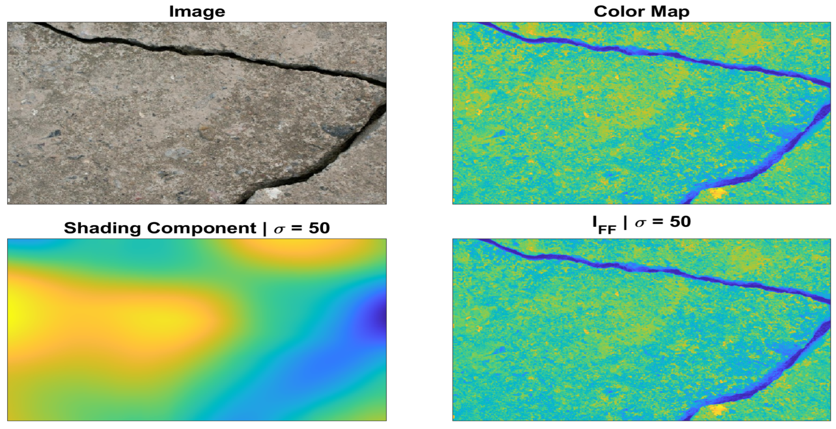
On the other hand, Figure 2 elucidates the effect of overestimation of sigma with a value of $\sigma =50$. In this case, it can be noticed how the shading component obtained using a big value of sigma produces uncorrelated values with respect to the position of the shadow/bright areas. This leads the resulting flat-fielded image to be close to the original image without much correction.

In order to solve this issue, the authors propose a new approach and assign the name PCA Gaussian to it. The methodology consists of creating a bank of Gaussian’s filtered images with different sigma values. Then, a principal component analysis (PCA) analysis allows obtaining the coefficients to combine the different levels into a unique feature, keeping the spatial information. The methodology is analogous to working with a multilevel pyramid scheme, in which the different levels detect different frequencies in the image.

Figure 3 shows the Gaussian bank for the presented example. It can be noticed how the details in the filtered image decrease as the sigma increases.

Figure 4 presents the results for this example. In the bottom left part of the figure, the resulting shading component obtained with the PCA Gaussian methodology is displayed. It can be appreciated how the new shading component combines the low- and the high-frequency components, yielding a better description of the brightness/shading phenomena. The bottom right part of the figure presents the corrected flat-fielded image. The result maintains the darkness within the cracks and corrects the brighter parts in the rest of the scene.

3.2. Textural Features Using Gabor Filters

Texture in the context of image analysis is considered as the regular repetition of an element or pattern on a surface. The use of textural features extracted with Gabor filters yields valuable extra information that can be used for many different purposes.

In this work, the goal is to extract the textural features with the Gabor filters in order to identify regions with different probabilities for cracks to develop. We follow the basic approach described in [52] to perform texture segmentation. Firstly, a bank of Gabor filters is designed using different frequencies ($\lambda$) and orientations ($\theta$). Each pair of frequencies and orientations localizes different information in the input image. Regularly sampled orientations between $0^{\circ }$ and ${150}^{\circ }$ in steps of ${30}^{\circ }$ are considered, while for wavelength, increasing powers of two starting from $4/\sqrt{2}$ up to the hypotenuse length of the input image are taken into account. These combinations of frequency and orientation are taken from [52]. Only the magnitude response of the filter is considered. The aspect ratio of Gaussian in the spatial domain ($\gamma$) defines the ratio of the semimajor and semiminor axes of the Gaussian envelope. This parameter controls the ellipticity of the Gaussian envelope. In this work, a value of $\gamma =2$ was found to yield better results due to the similarities between the elliptical shape of the filter and the cracks. Figure 5 shows the filter bank.

Each row represents the orientation of the filter and each column represents the wavelength. For a better representation, each kernel was resized, and on the top row for each column, the size of the kernel is shown. Furthermore, it can be noticed how the columns at higher frequencies are richer in detail.

Figure 6 closely shows the 30th filter, for the wavelength $\lambda =90.51$, orientation $\theta ={120}^{\circ }$, and aspect ratio $\gamma =2$. On the left side of the figure, the 3D shape of the filter can be appreciated.

In order to avoid local variations, each channel is filtered using a Gaussian low-pass filter to smooth the Gabor magnitude information. Sigma is chosen to match the Gabor filter that extracted each feature. A total of 36 features were extracted at different frequencies and orientations. Figure 7 presents one new example and exposes the result of the filtered response.

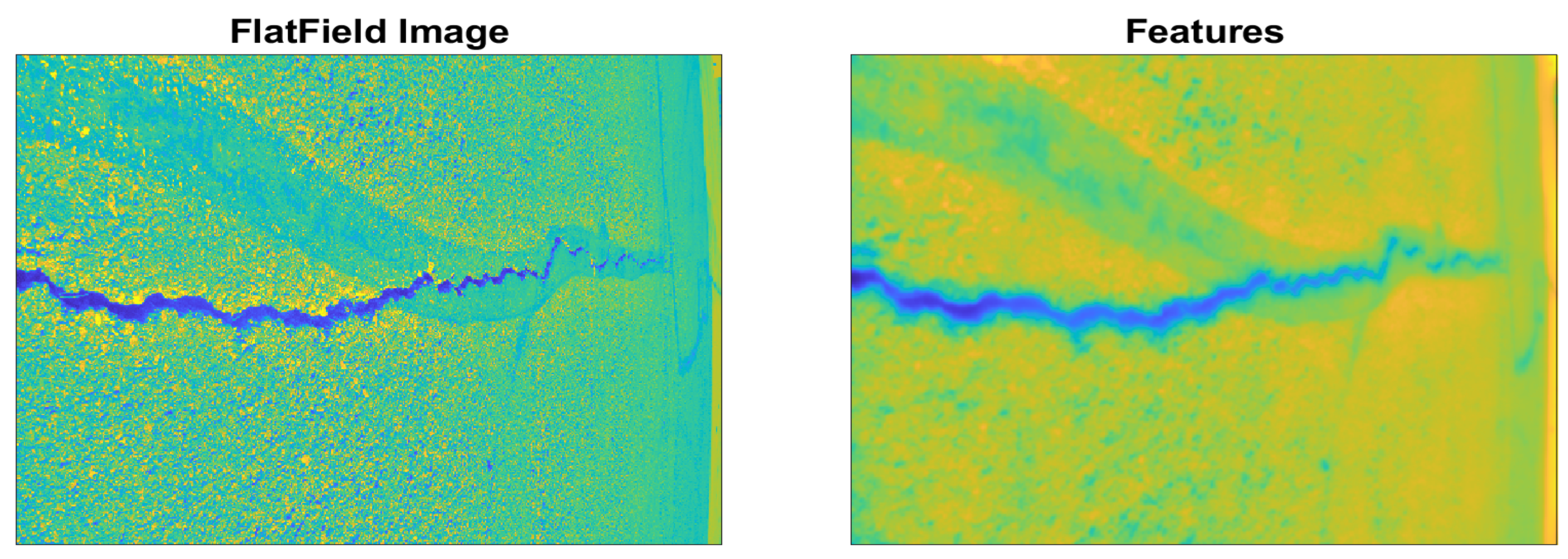
The resulting filtered magnitudes are concatenated in depth alongside the spatial information. This additional information help to group regions that are spatially closer. PCA is used to move from a 36D representation of each pixel in the input image into a 1D intensity value for each pixel. Figure 8 shows the output obtained for the example being analyzed.

Finally, we present in Figure 9 the difference between the Gabor features extracted on the original image against the Gabor features extracted from the flat-field corrected image. The longest wavelengths can influence the extraction of features whenever the global gradient of brightness is important, such as in the example presented. It is intuitive from the image to understand the effect the flat-field correction has on the results, yielding more pattern-orientated, rather than intensity-orientated, results. In other words, it gives more weight to the cracks/roughness rather than the gradient of intensities.

3.3. Local Minima

Local minima detection is the process where the lowest values of intensity are found within a small area. The minimum value is compared against a threshold obtained analyzing the statistics of the image. From [43], the window size was chosen to be $8\times 8$, which yields results that balance accuracy and computational time, while the threshold is obtained as follows: $S_a={\mu }_a-{\sigma }_a$, where ${\mu }_a$ is the mean intensity of the image and ${\sigma }_a$ is its standard deviation. Local minima detection is a key step in RB-MPS. Indeed, the detected local minima are used as nodes in the path finding algorithm. Therefore, an underestimation of the nodes leads to potential missed paths, and an overestimation leads to a higher concentration of short paths, which overloads the computational cost and biases the statistical estimation used for rejection. Moreover, a high concentration of nodes leads to a generation of closed paths. This issue is not considered in the previous version of the algorithm [42,43]. The new modifications proposed in this step of the study are mainly two:

∘

Minimal distance between two adjacent minima.

∘

Detection of local minima from two regions.

3.3.1. Adjacent Local Minima

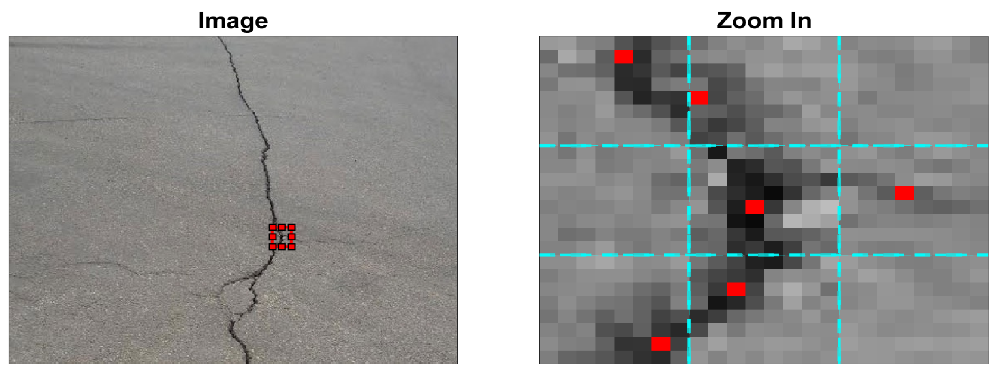
The procedure for the original local minima is presented in Figure 10 with a new instance from the dataset. As can be appreciated, the windows are represented by a grid in cyan color. The size of the window that has been already mentioned is $8\times 8$ and, inside each window, the minimum is marked with a red point. On the left side of the figure, the entire image is presented; a blue square indicates the zoomed-in area that is presented on the right side of the figure.

The adjacent local minima, or repulsion of nodes, is a minimal distance defined by the user in which the nodes cannot lay next to each other. To introduce this concept, Figure 11 is presented. The figure shows a synthetic gray image with all its values equal to $0.5$. A series of values lower than $0.5$ are presented with different colors, red, green, yellow, and blue, for the corresponding quadrants I, II, IV, and V. At the same time, each color has its own range of values from $0<I_{color}<0.5$, with the darkest being the lowest ones. On the right side of the figure, the local minima obtained with the original method are presented. As can be appreciated, the red and the dark green points end up lying next to each other.

Figure 12 presents the result obtained with the repulsion modification. The center image shows a minimal distance between adjacent points of 1 pixel, while the right image shows a minimal distance of 2 pixels.

In the present work, a minimal distance of $d_{min}=2px$ is adopted. Figure 13 compares the same image with the two methods. As can be appreciated, the repulsion method promotes a better alignment between points, as well as better coverage along the crack.

3.3.2. Region-Based Local Minima

The second part of this subsection is the region-based local minima. Using the extracted Gabor features, a segmentation is obtained in order to separate two areas based on their textural content. The local minima are found separately for each region. For the first region, the global local minima are calculated from the entire feature image using a global threshold $T_1={\mu }_{GF}-1.5{\sigma }_{GF}$, where ${\mu }_{GF}$ is the mean of Gabor features and ${\sigma }_{GF}$ its standard deviation, then only the points falling within the region with the lowest values from the Gabor features (Region 1) are maintained. For the second region, the flat-fielded image is used to determine the local minima; in this case, a regional threshold $T_2$ is obtained considering the values from Region 2 and is equal to $T_2={\mu }_{FF\cap R2}-2.5{\sigma }_{FF\cap R2}$, where ${\mu }_{FF\cap R2}$ is the mean of the intensity values from the flat-fielded image only in Region 2 and ${\sigma }_{FF\cap R2}$ its standard deviation. Finally, the union of these two points yields the local minima. Figure 14 shows the decisional flow chart used in this step.

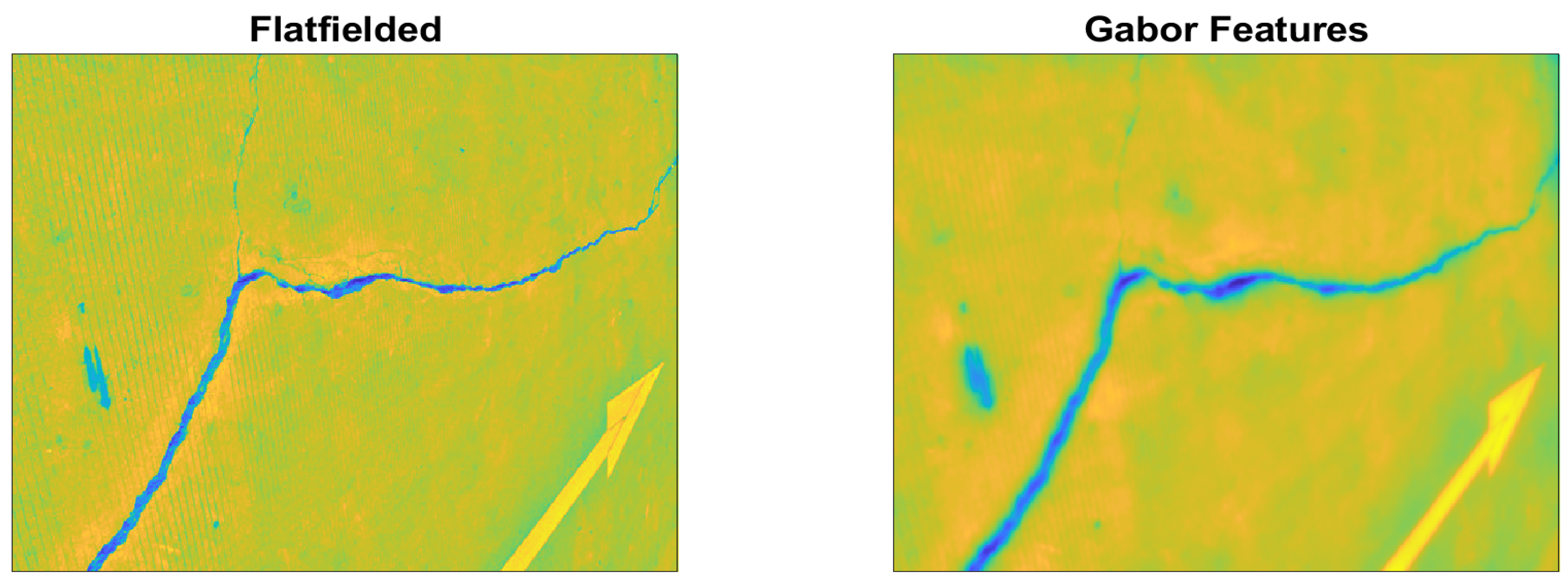
In the following Figure 15, we present the image used to illustrate the procedure. On the left side, the flat-fielded image is presented, while on the right side, the extracted Gabor features are presented. The Gabor features emphasize the area where the biggest crack is present, but it loses the definition of the finer details.

Based on this fact, the image is segmented into two areas from the textural features, as shown in Figure 16. To perform this, a K-means clustering-based algorithm for image segmentation was performed on the 36D image with all the magnitude responses concatenated in depth as well as the spatial coordinates. K was chosen equal to 3, then the lowest region was defined as Region 1 and the other two as Region 2. It can be appreciated on the right side of the image that the yellow label “Region 1” represents the potential position of the biggest cracks and the violet label “Region 2” represents the background of the scene.

Figure 17 shows, separately, the obtained points for each region. On the left side of the figure, the Gabor features extracted alongside the obtained points for Region 1 show the concentration of points falling within the big crack. On the right side, the flat-fielded image alongside the points found for Region 2 represent the background and therefore have a bigger constant equal to 2.5, compared with the 1.5 used for Region 1 in the feature image.

Subsequently, Figure 18 is presented, displaying a comparison between the original method and the proposed modification. As can be noticed, the proposed new method allows separating the identified local minima into two categories; on the right side of the image, the points coming from Region 1 are marked in red, while the ones coming from Region 2 are in green. Furthermore, the use of different constants for each threshold value gives more flexibility to the user who can adjust them depending on the particular case.

To highlight the importance of the flat-field correction when extracting the features, which then are used to segment the regions, the example from Figure 9 is recalled and displayed alongside the segmentation for each case in Figure 19. As can be noticed, on the right side of the image, the segmentation after correcting the brightness guides the segmentation to consider only the major crack.

Finally, Figure 20 is presented below; in this case, a new example is shown to expose the impact of the proposed methodology regarding the total number of points. As can be noticed from the image, the total amount of points is reduced almost two times compared to the original methodology, which mostly lies in the background area. As stated in the introduction of Section 3.3, the total number of points has a huge impact in terms of computational time when calculating the minimal paths between nodes.

3.4. Minimal Paths

The concept behind the minimal path selection is based on the theory of the Dijkstra algorithm already described in Section 2.1. Using the fundamental principles of graph theory, the minimal path between two nodes is found by defining a cost function. As already stated, cracks present a common property, i.e., they are usually formed in a shape of a line or a set of gridded lines that break the homogeneity of the surface. These breaks, having a fast rate of change in the slope of the surface, generate an obstacle for the incoming light which is seen by the human eye as a dark area. In other words, the cracks are generally captured in the images as the darkest areas and they follow a random path. Therefore, in the context of crack detection, the cost function to be minimized was defined, taking into account these considerations. The cost function was defined as follows:

$$c\left(p_{ij}\right)=\sum _{m=i}^{j}I\left(m\right)$$

(8)

where $c\left(p_{ij}\right)$ is the cost of the path from i to j, $x_i$ is the source point, $x_j$ is the destination point, and m is a pixel within the path; using this cost does not constrain the shape nor the length of the selected paths.

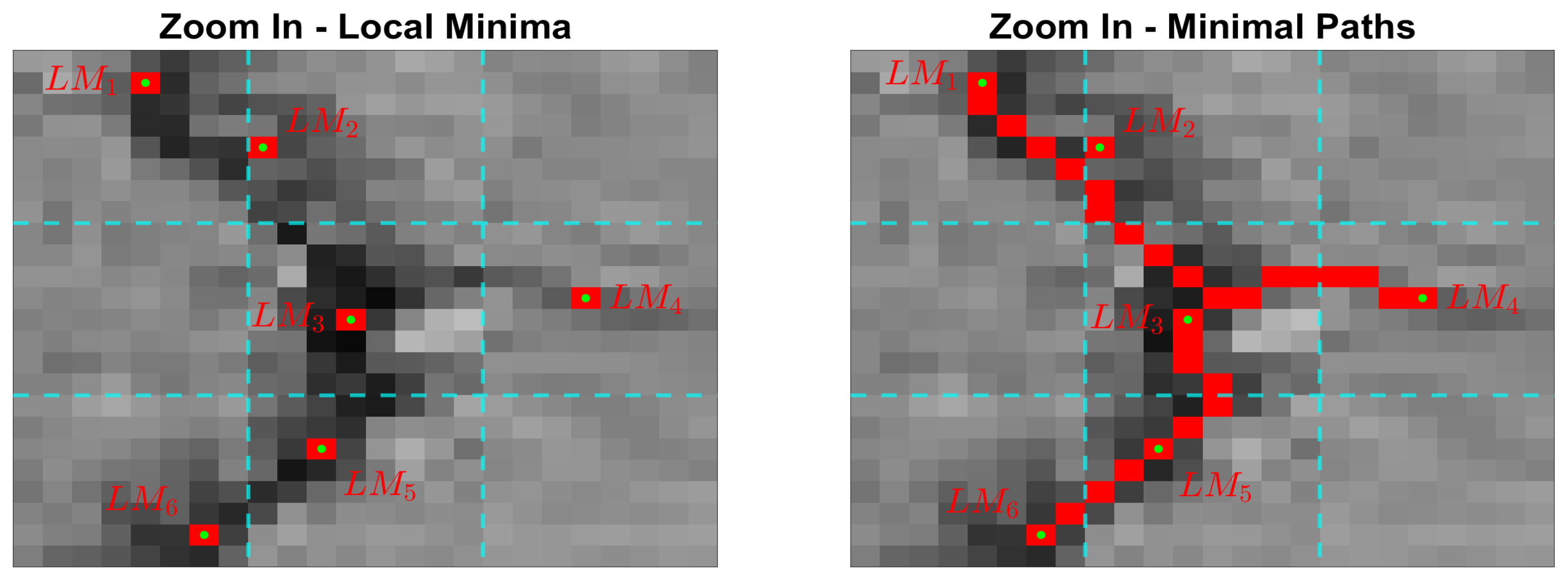
Figure 21 shows the image used to present the modifications in this section. On the right side, a zoomed-in portion is presented with the associated local minima. As can be appreciated, 6 local minima are present in the example.

An important aspect that is not clearly explained in [42,43] is the fact that some paths are overlapped, leading to a biased accumulation of the costs. In order to elucidate this issue, we analyze the total number of combinations. This number is obtained by calculating the number of possible combinations for each node to all the others. This is performed using Equation (9).

$${}_n^{}{\mathrm{C}}_k=\frac{n!}{\left(n-k\right)!k!}$$

(9)

where k is the number of combinations and n is the number of nodes. In this particular case, $n=6$ and $k=2$, since the nodes can only be set as start or end, and the total number of possible combinations $C=15$.

Figure 22 presents the same zoomed-in portion. On the left side of the image, the local minima can be appreciated, while on the right side, is the obtained minimal path.

Figure 23 presents the number of times a pixel is traversed along the path. As can be appreciated, all the pixels within the paths are at least crossed $n-1$ times, and the central is crossed 11 times. It is also important to notice that the window we are analyzing at this moment will be shifted; therefore, again, some paths will be considered twice. A solution to these problems is introduced in the next subsection.

3.5. Acceptance-Rejection of Paths

The next step in the algorithm foresees the acceptance or the rejection of the paths that satisfy a certain condition based on a defined limit. This threshold is estimated on the statistics of the so-far obtained paths. At this step, the goal is to select paths with the lowest mean intensities and not the shortest ones; therefore, the threshold is estimated with a normalized version of the cost by simply dividing the previous cost in Equation (8) by the length of the path:

$$c\left(p_{ij}\right)=\frac{1}{len\left(p_{ij}\right)}\sum _{m=i}^{j}I\left(m\right)$$

(10)

where $len\left(p_{ij}\right)$ is the length of the path in pixels. Then, the threshold is calculated as follows:

$$T_C={\mu }_c-k{\sigma }_c$$

(11)

where ${\mu }_c$ is the mean of the costs, ${\sigma }_c$ is their standard deviation, and $k=1$, which was determined empirically. Figure 24 shows the results obtained with the original method. On the left side of the figure, the image with the paths found is presented, while on the right side, the paths that satisfied the condition are displayed.

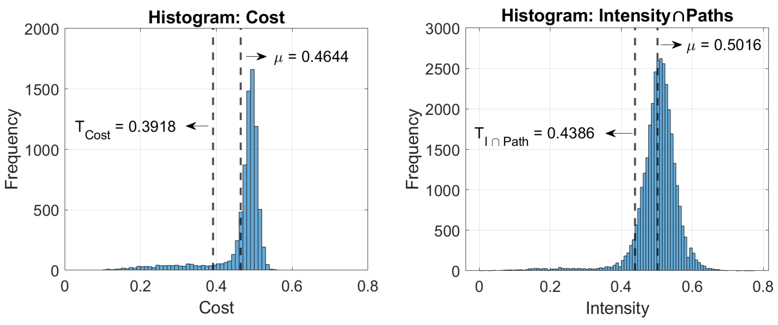
As anticipated in the previous subsection, a specific issue was identified in the procedure since some paths cross the same pixel several times. This fact influences the calculation of this threshold since the estimate is biased towards the deepest cracks that are traveled several times. Therefore, the threshold is overestimated while the found paths are underestimated. Two potential solutions addressing this issue are proposed. First, since the statistics of the cost function follow roughly a bimodal distribution, calculating the $T_c$ with Equation (11) shifts the value towards the darkest points in the image, and the solution is foreseen to determine the threshold based on a Gaussian fit on the upper mode.

Figure 25 shows a comparison between the threshold determined over the statistics of the Costs and the proposed Gaussian fit threshold. As can be noticed by the vertical dashed lines, the threshold in the original methodology is lower than the one proposed.

In the following Figure 26, results obtained with the original threshold and with the first solution are introduced. It can be noticed how this threshold covers more secondary cracks that in the first case are omitted.

The second solution proposes that the threshold can be obtained directly by considering the mean and standard deviation of the intersection between the image and the so-far detected paths, instead of calculating the cost for each path and estimating the threshold from the population of costs. In other words, it considers only the intensity levels of the detected paths. The threshold is named global threshold and is determined as follows:

$$T_{Global}={\mu }_{I\cap Paths}-k{\sigma }_{I\cap Paths}$$

(12)

where ${\mu }_{I\cap Paths}$ is the mean of the intensity levels of the so-far identified paths, ${\sigma }_c$ is their standard deviation, and $k=1$ remains the same as before. Figure 27 shows the histograms for both cases.

On the left side of the figure, the histogram of the costs is presented, while on the right side is the histogram of the intensities. It can be noticed in the latter how the histogram can be better fitted by a normal distribution. Indeed, this solution is the equivalent of considering the paths as traveled only once, since Equation (10) is no other than the mean intensity of the path.

Figure 28 shows a comparison between the paths obtained using the original cost threshold from Equation (11) vs. the global threshold from Equation (12). As can be noticed, the image from the right, corresponding to the global threshold method, yields results in between the original threshold method and the Gaussian fit method.

In the present new version of this algorithm, the global threshold is used following the methodology proposed in Section 3.3.2 for local minima. The region-based concept is also extrapolated for the calculation of the thresholds. Figure 29 presents the image and the identified regions.

For each region found in Section 3.3.2, a different threshold is calculated. The calculation of the thresholds follows the notions introduced in the previous section. This allows better control of the thresholds in the different zones. Particularly, the zone identified with the lowest feature values typically matches the biggest crack of the region. Therefore, the threshold for the paths falling within this region considers the addition of the standard deviation rather than the subtraction of it.

$$\left\{\begin{array}{c}{T}_1={\mu }_{I_1\cap Path{s}_1}-k_1{\sigma }_{I_2\cap Path{s}_2}\\ T_2={\mu }_{I_2\cap Path{s}_2}+k_2{\sigma }_{I_2\cap Path{s}_2}\end{array}\right.$$

(13)

where $k_1=1$ and $k_2=0.6$. Figure 30 presents the histograms for both cases. In the figure, the Y-axes are plotted in a logarithmic scale. In the figure, the upper histogram represents the methodology presented in Section 3.5, obtaining the threshold with Equation (11), while the lower graph presents two histograms, one for each region, and the determined thresholds for the particular example presented.

As can be noticed, the upper threshold is slightly higher than the global threshold, i.e., $T_{global}\le T_1$; this allows the detecting of a higher amount of cracks in the foreground. Furthermore, the lower threshold is slightly lower than the global one, i.e., $T_{global}\ge T_2$; this reduction helps to filter some of the paths falling within this area. Figure 31 shows the comparison of the paths found using the original, the global, and the region-based thresholds.

Analyzing the results, it can be appreciated how the proposed improvements yield a higher amount of true positives in the background area compared with the original methodology. Nevertheless, a higher amount of false positives is also present. It seems to indicate that the global methodology yields better results but, after this step, the original algorithm foresees a global skeletonization procedure and a crack length filtering. Therefore, short cracks are disfavored and the critical point in this algorithm obtains connected cracks.

3.6. Skeletonization and Region Growth

This two steps are foreseen in the original algorithm; this was introduced in Section 2.3 as steps 5 and 6, respectively. In this work, these two steps were kept unchanged. For the skeletonization step, two types of nodes are identified: branch points and end points. To determine them, an internal function from Matlab^®, called bwmorph, is used, both to skeletonize the paths and to find the points of interest.

The region growth procedure consists of iteratively absorbing dark pixels neighboring the currently detected crack, according to a threshold test. For further details, the reader is referred to [43].

3.7. Geometric Threshold

As a final step, a new filtering procedure on the found regions is proposed. Using an internal function from Matlab^®, called bwconncomp, two properties are analyzed for each connected region: area and eccentricity. While the definition of the first is redundant, the latter is a property measured on an equivalent ellipse that has the same second moments as the identified region. The elongation of that ellipse is measured by its eccentricity e, a number ranging from 0 to 1. A value of $e=0$ represents the limiting case of a circle, while a value of $e=1$ represents the limiting case of infinite elongation (no longer an ellipse but a parabola), in our case, a line segment. The eccentricity is calculated as follows:

$$e=\sqrt{1-\frac{b^2}{a^2}}$$

(14)

where a is the length of the semimajor axis and b is the length of the semiminor axis.

The combination of these two properties determines the regions to be filtered. The combination is shown in the following

Table 1. Properties.

Category	Area	Eccentricity
I	10–25	0.975
II	25–50	0.950
III	50–250	0.900
IV	>250	0.850

.

4. Results

Figure 32 shows the results obtained for four different examples. For each image in the figure, the main cracks were presented in green, the secondary cracks in blue, and the filtered regions in red.

In all four images, the green cracks represent the main crack belonging to Region 2 defined in the previous sections. Cracks displayed in blue represent secondary cracks belonging to Region 1. In red, the small regions filtered in this last step can be appreciated. In A, the image presents a perspective view, the image presents thin cracks and several secondary cracks, and three small regions were filtered belonging to Category III from Table 1. In B, a wide crack is presented; as can be noticed, this type of crack yields results not as good compared with the other cases, and the detection of secondary cracks is not accurate. Moreover, the image present a watermark, which elevates the complexity of the scene; the images with watermarks were chosen to be left in the dataset since they represent a typical challenge that DL models solve quite well. In C, a crack with medium width and with a short secondary crack is presented, and several small regions belonging to Category I are rejected. Finally, in D, an image with a view from the top is presented; in the scene, a big oil stain can be appreciated together with a main thin crack: the big oil stain belongs to Category IV and is rejected since it does not fulfill the eccentricity criteria.

A and D present a particular situation regarding the blue areas, i.e., the secondary cracks. It can be noticed that some small parts of the blue areas indeed belong to the primary or main crack. In order to adjust this, blue regions are analyzed as to whether they fall within a green crack or not. In the case that they fall within a green crack, they are considered as if they were part of it and they are absorbed. On the other hand, blue regions having free endpoints are retained as secondary cracks together with disjointed areas. Figure 33 highlights the incorporation of blue segments to the green ones. In addition, some secondary cracks growing from the main crack are retained and some other unconnected areas are present.

Finally, Figure 34 shows the comparison between the results obtained with our method RB-MPS and the original MPS algorithm. The presented examples are displayed vertically and each method is represented on each column, respectively. Images A, C, E, and G present the results with RB-MPS while B, D, F, and H present the results obtained with MPS.

In the first row, it can be appreciated how the MPS algorithm has good accuracy regarding the main crack. However, the detected secondary cracks of A are omitted in B. The next row presents an example of a wide crack; as can be seen, the MPS methodology does not detect any crack. This is due to the distribution of pixel intensities since the present image contains a high number of dark pixels belonging to the crack. Therefore, at the moment to accept paths, none of them satisfy the condition and become rejected. On the other hand, the result obtained with RB-MPS is not optimal, but the region-based approach allows them to keep the paths and still finds a good amount of paths inside the crack. Continuing downwards, the following row presents images E and F. In this case, the detection with MPS is not quite accurate since some internal parts within the crack are missing, while the result with RB-MPS shows a really good performance. Finally, images G and H present the last example. In this case, the results in H show a big stain detected as a crack, while, as shown in Figure 33, the stain is filtered in the last step of the procedure.

In order to provide a quantitative comparison, a set of evaluation metrics are used to assess the performance of the results. These metrics measure the similarity between the predicted and the ground truth regions based on the number of true positives (TP), true negatives (TN), false positives (FP), and false negatives (FN) generated by the model. Precision, recall, and F1-score are commonly used metrics for binary classification tasks and are widely used in crack segmentation.

∘

Precision: Precision measures the proportion of true positives among the predicted positive samples. Precision is a useful metric when the cost of false positives is high, such as in medical diagnosis. It is calculated as follows:

$$Prec=\frac{TP}{TP+FP}$$

(15)

∘

Recall: Recall measures the proportion of true positives among the actual positive samples. Recall is a useful metric when the cost of false negatives is high, such as in fraud detection. It is calculated as follows:

$$Rec=\frac{TP}{TP+FN}$$

(16)

∘

F1-Score:F1 is the harmonic mean of precision and recall and is used to balance the trade-off between them. F1-score is a useful metric when both false positives and false negatives are equally important, and there is an imbalance in the class distribution. It is calculated as follows:

$$F1=\frac{2·Prec·Rec}{Prec+Rec}$$

(17)

A distance of 2 pixels between the detection and the reference segmentation for the calculation of the TP rate is accepted in the same manner as in [43].

Table 2. Metrics RB-MPS vs. MPS.

	Precision		Recall		F1
	RB-MPS	MPS	RB-MPS	MPS	RB-MPS	MPS
Find Paths	0.3133	0.1346	0.9541	0.8785	0.4255	0.1505
Clean Paths	0.7019	0.4695	0.9105	0.7455	0.7626	0.3162
Skeleton	0.7692	0.5412	0.9472	0.8263	0.8100	0.4944
Final	0.8144	0.5694	0.9407	0.8102	0.8386	0.5536

shows the mean of the metrics obtained at each step of the procedure for both methodologies. As can be noticed in every single step, our RB-MPS outperforms the MPS. It is important to note that the biggest differences can be seen in the first two steps of the procedure. Indeed, this is a combined consequence of the lower number of local minima and the region-based rejection strategy.

Table 3. Metrics MPS vs. RB-MPS vs. DC.

	Precision	Recall	F1
MPS [42,43]	0.5694	0.8102	0.5536
RB-MPS	0.8144	0.9407	0.8386
DC [50]	0.8610	0.8690	0.8650

displays the results compared against the results presented in DeepCrack. It can be noticed how the deep learning approach yields better results in terms of precision, while our approach has a higher recall value. A high recall value means that the number of FN is quite low, while a higher value of precision translates into a lower number of FP. It can be noticed in the case of the DC approach how the recall and precision values are more balanced, while in our approach this difference is slightly more acute. The explanation behind this difference is mainly due to the incorporation of the secondary cracks in our approach, which yield a higher number of FP, impacting the precision rate value.

In order to give a visual demonstration, Figure 35 is presented. The figure shows a comparison of the results obtained with the different methods. The first row presents the original images extracted from the dataset. Then, the second row named B, presents the ground truth data which were labeled by hand by experts. The third row, named C, shows the results obtained with the DeepCrack network. Row D presents the results obtained with the MPS algorithm. Finally, row E shows the results obtained with the RB-MPS. The results obtained with RB-MPS perform slightly worse in situations where the crack width is considerable, such as the first column case. On the other hand, the MPS algorithm completely fails to identify this type of crack. The second and third column examples show how the DC has a continuous estimation map, i.e., nonbinary, yielding an effect of degrading. Regarding MPS vs. RB-MPS, the results are quite similar, with a slightly higher rate of false detection coming from the MPS. Finally, the last example in the fourth column shows an exogenous flower in the middle of the crack. In this case, our algorithm outperforms DC and MPS. Further discussion can be found in the next section.

5. Discussion and Future Works

Even though the Results section showed a couple of examples of the final results, through Section 3, different steps from the proposed new version of this algorithm were introduced along with some results.

Table 4. Steps MPS vs. RB-MPS.

	MPS [42,43]	RB-MPS	Upgrade
Preprocessing	No Details	Flat-Field	New
Kernel	8 × 8	8 × 8	Same
Local Minima	Global	Adjacent Gabor-Region-Based	New
Paths Finding	Dijsktra	Dijsktra	Same
Rejection	Global	Region-Based	New
Skeletonization	Branch and Loops	Branch and Loops	Same
Width Grow	Absorption	Absorption	Same
Geometric Threshold	No	Yes	New

resumes the differences in the steps, comparing the original algorithm and the proposed one.

Starting from the top, the first row highlights how the original algorithm does not present any details regarding the preprocessing step used. In this study, a new flat-fielded methodology was proposed. The new Gaussian PCA was proven to improve the accuracy of the new algorithm through the workflow and in the final outcomes. This step is rarely made explicit or detailed; even with deep learning approaches, this preprocessing step is taken for granted, even though it has a big impact on the following steps.

Secondly, the kernel dimensions influence the computational time of the Dijkstra minimal path search, since the distance between nodes increases. Moreover, too-small window sizes can yield unconnected paths, which is undesired since small paths are removed. Therefore, the kernel size was left unchanged based on the results shown from [43].

Third, the local minima present two new improvements. First, the adjacent repulsion allows the local minima not to be placed side by side, and, thus, they better cover the crack length. This improves the path connections which otherwise are at risk of becoming detached. Secondly, the segmentation obtained by using Gabor filters allows two regions to be distinguished. These regions give rise to the new region-based approach. In this particular step, the new approach yields a lower number of local minima, i.e., nodes in the algorithm; therefore, this number has a huge impact on the computational time. The lower quantity of points is more visible in the background, meaning that the new approach keeps the points laying in the main crack while reducing the amount of them in the background zone.

Next, for the rejection/acceptance of the paths, an important problem was detected. Indeed, the original version of the algorithm overestimated the threshold since the statistic calculated over the cost considered paths traversing some pixels several times, biasing the threshold towards the darkest values; this resulted in some neglected secondary cracks. The region-based approach was incorporated to overcome these problems, and this aspect became one of the main advantages of our work since the algorithm is able to better identify secondary cracks. Furthermore, another big issue was identified in cases where the crack represented a high proportion of the scene, such as the wide cracks or close-up images. The problem was corrected by considering the global thresholding approach for each region; this is a key concept that allowed us to overcome these problems and better generalize the algorithm.

Concerning the minimal path finding algorithm, i.e., Dijkstra, the skeletonization and the width growth, no further modifications were introduced, and the same concepts described in the original algorithm hold. As a final step, the geometric threshold step was incorporated; this step is very important since the overestimated regions are filtered, such as in the case of rounded shape objects or very short thin cracks.

Finally, the results showed close to state-of-the-art results using deep learning approaches. From a quantitative point of view, the metrics from the DC showed a slightly higher F1-score, yielding more balanced precision and recall metrics. In the case of MPS, the final F1-score is quite low; this is mainly explained because the algorithm was developed for thin cracks captured with a zenithal camera. Therefore, in this case, where the dataset was complex and had a lot of variance, several cases, such as the one presented in the first column in Figure 35, failed to detect any crack. On the other hand, our RB-MPS algorithm was developed to overcome this problem and to better generalize the results. This is clear from the metrics results; however, the in-balance that can be seen in between the precision and recall indicates that the algorithm tends to yield a higher value of FN than FP. Particularly, a higher number of FPs influence the precision, yielding lower values, but as already stated, the ground truth labeling often neglects the secondary cracks, therefore our RB-MPS algorithm yields lower values of precision compared with the DC. This problem is recurrent in other crack databases since the labeling procedure is carried out manually with a high subjectivity from the expert. The authors believe that this issue must be deepened and studied in order to obtain a more standardized procedure for crack labeling.

A clear visual demonstration is presented in Figure 35, and the results obtained with RB-MPS perform slightly worse in situation where the crack width is considerable, such as in the first column case. The reason behind this behavior is the kernel size and the region-growth procedure. This problem open the possibilities for future work and can be easily tackled using a multilevel tackled scheme to estimate cracks at different scales. Following the discussion of Figure 35, the results presented for the DC showed a continuous estimation map of the crack; this can be explained due to the choice of the weighted cross-entropy loss, in terms of probability, that combines the outputs at each side with the final fused estimation. This concept is interesting and could be exploited in order to fuse both approaches, opening the field to interesting new results.

On the other hand, still referring to Figure 35, it was interesting to notice how the new addition, regarding the geometric threshold to determine the regions to be filtered, allowed the exclusion of exogenous elements in the images, such as the flower in the corresponding figure, or the oil stain in Figure 32. This is an excellent improvement, but must be calibrated carefully since it is scale-dependent. The values presented in this work were calibrated to yield the best results with the current dataset.

The main downside of the current algorithm is the computational speed. Indeed, the current algorithm speed is dependent on the total number of local minima found. On average for the dataset, the total time for each image sized 544 × 384 is about 65 s using the suggested parameters. In addition, in the case of not-satisfactory results, the calibration for the optimal parameters requires the user to supervise the algorithm for each instance. In the case of a large amount of data, an advised workflow is the following: run the entire dataset with the suggested parameters, check for unsatisfactory results, and adjust the parameters in order to obtain the desired results.

Here, the typical discussion between traditional and deep learning approaches opens up once again. Indeed, both methodologies have their advantages and drawbacks. For this particular application, DL models yield more balanced results and with higher metrics values (F1). However, they are usually solved using supervised learning, meaning that a lot of labeled data are needed, which is a tedious, prone-to-error, and time-consuming task. Furthermore, the “black-box” nature of the DL makes them indecipherable and impossible to correct when the results are erroneous. Conversely, the proposed “traditional” approach yields slightly lower metric values for the particular dataset. Nevertheless, these metrics could be biased since the current algorithm does not consider secondary cracks; hence, the values are lower. However, the main advantage of the proposed methodology is its transparency and its parametric nature, meaning that it could be adapted for each particular case and corrected in case the results are not satisfactory.

6. Conclusions

Cracks are fractures or breaks that occur in materials such as concrete, metals, rocks, and other solids. Cracks have an intrinsic randomness that makes them unpredictable and hard to model and assess. This aspect makes image-based methodologies very suitable and appropriate for the task of automatic detection systems. Although machine and deep learning algorithms have demonstrated their potential in the last decade, their “black-box” nature remains a gap to be filled in order to clearly explain the underlying principles of the phenomena under investigation or to assess counterintuitive outcomes. At the cost of losing computational efficiency, traditional image processing can track intermediate processes and can serve as a valuable tool for crack segmentation.

The present study proposed a framework for a new algorithm for crack segmentation based on the theory of minimal path selection combined with a region-based approach obtained through the segmentation of texture features extracted using Gabor filters. Starting from the concept introduced in [43], several modification were proposed in order to generalize the algorithm. Firstly, a preprocessing step was incorporated in order to homogenize the scene in terms of light and shadows. This preprocessing step improved the false rate detection of local minima, yielding a lower amount of points, which translates into lower computational burden at the time to calculate the path between nodes. Moreover, a slight modification in the local minima identification forced adjacent points to respect a minima distance, breaking the local accumulation of points in certain areas, thus homogenizing the distribution of detected points in the scene. Afterward, a region-based segmentation technique was introduced to determine two regions in the image: one with the potential position of the crack, and the second region considering the background. This region-based approach was a key improvement that enhanced the detection of secondary cracks and improved the rejection of false paths and the generalization of the algorithm, particularly for close-up scenes or wide cracks. Finally, a thresholding step based on geometrical properties was presented, allowing for excluding rounded areas and small isolated cracks.

The main advantage of this study is the transparency of the workflow, contrary to what happens with deep learning approaches. This transparency allows understanding and correcting outcomes in cases where the algorithm does not work correctly. Moreover, in order to use the deep learning frameworks, a huge amount of data is needed and each instance needs to be labeled by hand. In the proposed approach, prior information is not required. However, the statistical parameters may have to be adjusted to the particular case and requirements of the situation. The proposed algorithm results in a useful tool for researchers and practitioners needing to validate their results against some reference or needing labeled data for their models. Moreover, the current study could establish the grounds to standardize the procedure for crack segmentation with a lower human bias and to speed up the procedure. The direct application of the methodology to images obtained with any low-cost sensor makes the proposed algorithm an operational support tool for authorities needing crack detection systems in order to monitor and evaluate the current state of infrastructures such as roads, tunnels, or bridges.