Estimation of Instantaneous Air Temperature under All-Weather Conditions Based on MODIS Products in North and Southwest China

Abstract

Air temperature ($T_a$) is a common meteorological element involved in many fields, such as surface energy exchange and water circulation. Consequently, accurate $T_a$ estimation is essential for the establishment of hydrological, climate, and environmental models. Unlike most studies concerned with the estimation of daily $T_a$ from land surface temperature, this study focused on the estimation of instantaneous $T_a$ from Moderate Resolution Imaging Spectroradiometer (MODIS) atmospheric profile products aboard the Terra and Aqua satellites. The applicability of various estimation methods was examined in two regions with different geomorphological and climate conditions, North and Southwest China. Specifically, the spatiotemporal trend of $T_a$ under clear sky conditions can be reflected by the atmospheric profile extrapolation and average methods. However, the accuracy of $T_a$ estimation was poor, with root mean square error (RMSE) ranging from 3.5 to 5.2 °C for North China and from 4.0 to 7.7 °C for Southwest China. The multiple linear regression model significantly improved the accuracy of $T_a$ estimation by introducing auxiliary data, resulting in RMSE of 1.6 and 1.5 °C in North China and RMSE of 2.2 and 2.3 °C in Southwest China for the Terra and Aqua datasets, respectively. Since atmospheric profile products only provide information under clear sky conditions, a new multiple linear regression model was established to estimate the instantaneous $T_a$ under cloudy sky conditions independently from atmospheric profile products, resulting in RMSE of 1.9 and 1.9 °C in North China and RMSE of 2.5 and 2.8 °C in Southwest China, for the Terra and Aqua datasets, respectively. Finally, instantaneous $T_a$ products with high accuracy were generated for all-weather conditions in the study regions to analyze their $T_a$ spatial patterns. The accuracy of $T_a$ estimation varies depending on MODIS datasets, regions, elevation, and land cover types.

1. Introduction

Air temperature ($T_a$), typically measured at a sheltered height of 2 m above ground level [1], is a crucial parameter in various applications such as vector-borne disease bionomics [2], hydrology [3], and climate change [4,5]. $T_a$ is principally obtained from observations of ground-based meteorological stations with high temporal resolution and accuracy [6]. However, it can only cover a limited spatial range and cannot accurately reflect the spatial heterogeneity of $T_a$, especially in areas with significant variations in climate and altitude. Regional-scale distribution patterns of $T_a$ are easily obtained by interpolation, such as the inverse distance weighted, kriging, and spline methods [7,8]. However, it is difficult to generate high-accuracy $T_a$ data by these methods due to the limited number of stations in areas with complex natural environments and scarce meteorological data [9,10,11].

Compared with ground-based observation products, remote sensing satellites provide continuous surface and atmospheric parameters over a large region, resulting in temporal and spatial distribution data of $T_a$ [12]. Generally, remote-sensing-based $T_a$ estimation methods can be divided into four groups. The first category is the temperature-vegetation index (TVX), which is based on the assumption that the temperature of dense vegetation is in equilibrium with $T_a$ within the canopy [13,14]. This method establishes a negative correlation between land surface temperature (LST) and vegetation index (VI); the saturated VI value is then utilized to estimate $T_a$. The shortcomings are the need to remove excess cloud or water body information within the window and the consequent uncertainties when applied to areas with sparse vegetation [15]. The second class is the energy balance method, which utilizes the energy conversion process to estimate $T_a$ based on the surface heat flux balance equation [16,17]. The main drawback of this method is its complexity and the requirement for numerous parameters. It is difficult for remote sensing technology to simultaneously provide information on multiple parameters, especially in a large-scale region [18]. According to the principle of energy balance, the $T_a$ can also be estimated by using the energy conservation equation in the local scale mesoscale model [19,20]. It can consider various thermodynamic processes in the atmosphere and solve the $T_a$ distribution through numerical algorithms. However, it has disadvantages in estimating $T_a$, such as low resolution and difficulties in collecting and transmitting meteorological data. Thirdly, statistical analysis methods such as simple and multiple regression models can explore the relationship between $T_a$ and other variables directly. Their advantages lie in model simplicity and convenient application [21,22,23]. Fourthly, some studies utilized machine learning methods such as random forest, neural networks, and support vector machines to estimate $T_a$ accurately from remote sensing data [24,25,26]. Such studies usually require more computing resources and time. In addition, machine learning methods are usually black-box models, which are inadequate to provide a clear explanation of the relationship between model inputs and outputs. Therefore, the simple and intuitive linear regression models were adopted in this study, aiming to reflect the contribution of each variable to the output more directly.

Moderate Resolution Imaging Spectroradiometer (MODIS) datasets have been widely used in the $T_a$ estimation approaches mentioned above. Most of them are based on LST provided by MOD11A1 and MYD11A1 products [27,28]. For instance, Yoo et al. [6] applied LST to estimate the daily maximum and minimum $T_a$ for two megacities. In contrast, fewer studies have focused on the atmospheric profile products provided by MOD07_L2 and MYD07_L2. Some studies showed the potential advantage of MODIS atmosphere profile products to estimate $T_a$. Bisht et al. [29] proposed an approach to estimate $T_a$ based entirely on MOD07_L2 atmospheric profile products through the linear relationships between $T_a$ and altitude for different air pressure zones. $T_a$ of Limpopo River was estimated by utilizing MOD07_L2 atmospheric profile products and applying the vertical lapse rate of $T_a$ [30]. Unfortunately, the remote sensing data of this approach were affected by cloudiness and were only applicable to clear sky conditions. $T_a$ in the east part of the Qaidam Basin in China and the Southern Great Plains in the USA under all-weather conditions was estimated by Zhu et al. [31] based on the MODIS atmospheric profile products and LST provided by MOD06_L2.

The effectiveness of the atmospheric profile products in $T_a$ estimation has been demonstrated in different areas [32]. However, its adaptability in large-scale complex subsurface conditions still lacks effective validation and comparative analyses among different methods. Additionally, the study areas were small, and the climate and elevation changes in the regions were not prominent. Therefore, this study evaluated the applicability of the estimation scheme in two areas with completely different topography and climate conditions. Apart from verifying the applicability of the atmospheric profile products, this study is committed to further improving the accuracy of $T_a$ estimation. So far, the linear regression model is one of the most popular statistical models for estimation using MODIS products [33,34,35]. Therefore, high accuracy $T_a$ was expected by a multiple regression method in combination with LST products and other auxiliary datasets.

Since atmospheric profile products can only provide $T_a$ information under clear sky conditions, $T_a$ estimation under cloudy sky conditions is a crucial focus of this study. The instantaneous $T_a$ under cloudy sky conditions was estimated by simple and multiple linear regression models. Moreover, the instantaneous $T_a$ under all-weather conditions and the spatial distribution patterns of $T_a$ in the study areas were analyzed. Meanwhile, the study incorporated two different datasets from the MODIS sensors onboard the Terra and Aqua satellites to explore the influence of datasets on estimation accuracy.

The instantaneous $T_a$ is vital for meteorological processes and weather forecasting due to its near-real-time characteristics. Additionally, the instantaneous $T_a$ at the moment of satellite overpass is the basis for determining other daily temperature statistics [36]. It provides indispensable inputs to remote sensing models for evapotranspiration [37], net radiation [38], and soil moisture [39]. However, this study found that previous studies have mainly focused on daily minimums and maximums or the average $T_a$ over a given period [6,21,35,40], with little attention paid to the estimation of instantaneous $T_a$. Consequently, the primary focus of this study is to estimate instantaneous $T_a$ at the time of satellite overpass under clear and cloudy sky conditions.

In summary, the main objectives of this paper were the following: (1) to verify the applicability of atmospheric profile products in the estimation of instantaneous $T_a$ under clear sky conditions and enhance the accuracy of estimation by introducing LST and auxiliary data; (2) to estimate the instantaneous $T_a$ under cloudy sky conditions using regression methods, generate the instantaneous $T_a$ under all-weather conditions in the study area and analyze its spatial distribution pattern; (3) to compare the applicability of different estimation approaches and the difference in instantaneous $T_a$ estimation based on the Terra and Aqua datasets; and (4) to apply the estimation methods to two regions with entirely different topography and climate factors (North and Southwest China) to verify the applicability of the parameterization scheme.

2. Study Area and Materials

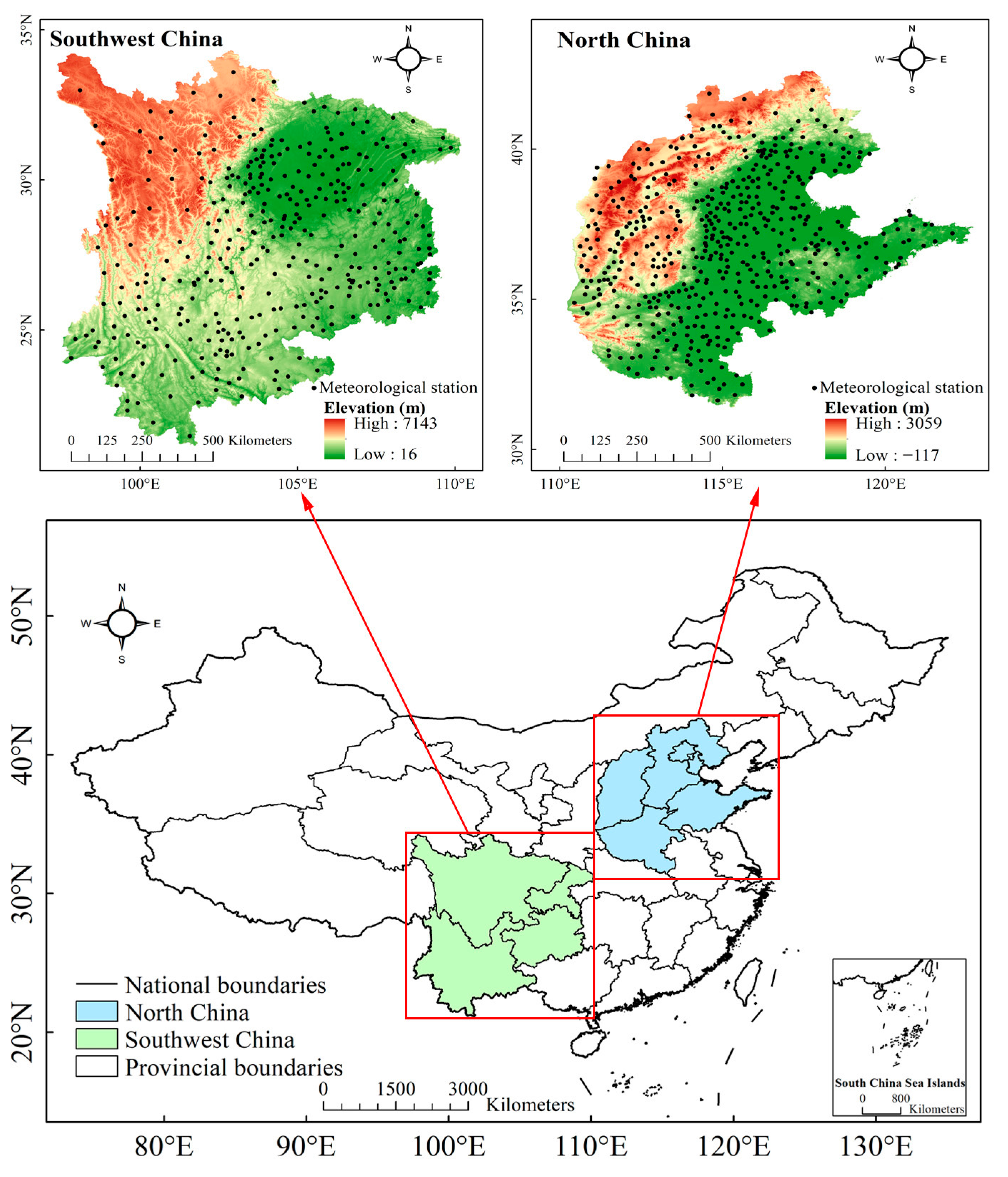
2.1. Study Area

The present study was conducted in two regions, namely North and Southwest China, with completely different geomorphological and climatic conditions (Figure 1).

2.1.1. North China

The definition of North China differs slightly according to the source. In this study, according to the administrative division, the Shanxi, Shandong, Hebei, and Henan provinces and the cities of Beijing and Tianjin were classified into North China [41]. The latitude and longitude range is 110°15′–122°43′E and 31°23′–42°37′N, respectively. North China is a semi-humid region with a temperate continental monsoon climate. Precipitation is unevenly distributed during the year and primarily occurs in summer [42]. Its northern and western regions are mountainous, and the vegetation types are mainly woodland and grassland; the central and eastern regions are extensive plains and represent the main crop production areas in China [43,44].

2.1.2. Southwest China

In this study, the southwest region, excluding Tibet, was selected as the study area (97°21′–110°11′E, 21°03′–34°19′N). It includes the Sichuan, Yunnan, and Guizhou provinces and Chongqing city, with a total area of approximately 10.5 × 10⁵ km². Southwest China has a complex topographic structure with plateaus and mountains [45]. The terrain is high in the west and low in the east [46]. The climate of the region is dominated by the subtropical monsoon climate, tropical monsoon forest climate, and the unique plateau climate of the Tibetan Plateau [47]. In addition, the vertical climate varies, and the annual precipitation decreases from southeast to northwest.

2.2. Datasets

2.2.1. MODIS Datasets

The remote sensing data for this study were obtained from the MODIS Terra and Aqua satellites with overpass times of approximately 10:30 a.m. and 1:30 p.m. (local time), respectively. Specifically, the MOD03, MOD06_L2, MOD07_L2, and MOD13_A2 products correspond to the Terra satellite platform, while the MYD03, MYD06_L2, and MYD07_L2 products correspond to the Aqua satellite platform.

The MOD07_L2 and MYD07_L2 atmospheric profile products include the atmospheric temperature profiles and the surface pressure distribution with a spatial resolution of 5 km [48]. The temperature profiles are distributed through 20 vertical atmospheric pressure levels (5, 10, 20, 30, 50, 70, 100, 150, 200, 250, 300, 400, 500, 620, 700, 780, 850, 920, 950, and 1000 hPa). They are determined through regression based on the statistical relationship between observed radiances and the corresponding atmospheric profile. However, MOD07_L2 and MYD07_L2 products can only provide temperature profiles and surface pressure under clear sky conditions. The MOD06_L2 and MYD06_L2 products contain optical and physical parameters of clouds that are used to determine cloud properties. Unlike MOD11A1 or MYD11A1 products, the LST is available in the MOD06_L2 and MYD06_L2 products for both clear and cloudy sky conditions. The LST data in the MOD06_L2 and MYD06_L2 products, with a spatial resolution of 5 km, is derived from the MOD11_L2 and MYD11_L2 products, National Centers for Environmental Prediction (NCEP) grid analysis, and Data Assimilation Office (DAO) data [29]. Bisht et al. [29] verified the LST obtained from the MOD06_L2 product against ground measurements. Their results showed that the RMSEs of daytime and nighttime LST estimates from the MOD06_L2 are 3.80 and 2.54 K, respectively. Thus, in this study, the LST was retrieved from MOD06_L2 and MYD06_L2 rather than MOD11A1 and MYD11A1 products. The solar zenith angle (SZA) was extracted from MOD03 and MYD03 products with a spatial resolution of 1 km. Additionally, the 16-day Normalized Difference Vegetation Index (NDVI) was extracted from the MOD13A2 product with a spatial resolution of 1 km.

2.2.2. Meteorological and Digital Elevation Model Datasets

Two additional datasets—Shuttle Radar Topography Mission’s digital elevation model (SRTM DEM) product and a meteorological dataset—were also employed. Specifically, hourly $T_a$ observations from 502 national meteorological stations in North China and 364 stations in Southwest China were used. Since the target of this study was the estimation of instantaneous $T_a$, only the $T_a$ observations closest to the Terra and Aqua satellites’ overpass time were used. It should be noted that the measurement errors of the meteorological dataset may have a potential impact in assessing the accuracy of the $T_a$ estimation. Measurement errors may increase the discrepancy between the estimated and actual $T_a$. The data quality has been preliminarily controlled by the data providing platform. The elevation was obtained from the SRTM DEM dataset, which has a spatial resolution of 90 m. To facilitate the analysis of the spatial distribution pattern of $T_a$ in combination with MODIS products, it was resampled using the nearest neighbor method to match the spatial resolution of the MODIS products.

3. Methodology

In this study, we adopted and compared different methods for the estimation of instantaneous $T_a$ from MODIS products and auxiliary data. Specifically, the approaches for $T_a$ estimation under clear sky conditions are the atmospheric profile extrapolation, average, and multiple linear regression methods. Meanwhile, the approaches for $T_a$ estimation under cloudy sky conditions include the simple and multiple linear regression models. The atmospheric profile extrapolation and average methods for clear sky $T_a$ and the simple linear regression for cloudy-sky $T_a$ were entirely based on MODIS products without any auxiliary data. As for the multiple linear regression method, auxiliary data, such as $T_a$ observations and the DEM dataset were introduced as input information under clear and cloudy sky conditions.

3.1. Estimation of Instantaneous $T_a$ under Clear Sky Conditions

3.1.1. Atmospheric Profile Extrapolation

The atmospheric profile extrapolation method estimates $T_a$ based on the linear relationship between $T_a$ and altitude at different pressure levels. Bisht and Bras [29] assumed that the vertical decrement rate of $T_a$ is 6.5 K·km⁻¹. However, the $T_a$ decrement rate has spatial and temporal variability, meaning that setting it as a constant would result in significant errors. Therefore, the method of Zhu et al. [31] was applied in this study. They estimated the direct temperature decrement rate by the temperature difference and the atmospheric pressure difference between the two atmospheric layers closest to the surface in the MOD07_L2 product. This effectively overcomes the limitations of the Bisht and Bras method. The calculation can be expressed as follows:

$$T_{a1,clear}=T_a^{L1}+\frac{T_a^{L2}-T_a^{L1}}{P_a^{L2}-P_a^{L1}}\left(P^S-P^{L1}\right)$$

(1)

where $T_{a1,clear}$ is $T_a$ retrieved by the atmospheric profile extrapolation method, $P^S$ is the surface pressure level obtained from MOD07_L2 or MYD07_L2 products, $P^{L1}$ is the lowest pressure level of the MOD07_L2 or MYD07_L2 products in this study, $P^{L2}$ is the nearest level above $P^{L1}$, and $T_a^{L1}$ and $T_a^{L2}$ are the atmospheric temperatures retrieved at a pressure level $P^{L1}$ and $P^{L2}$, respectively.

According to the surface pressure value of each pixel, the 16th–20th pressure levels of the atmospheric profile products corresponded to North China, and the 13th–20th pressure levels corresponded to Southwest China. In addition, many studies directly selected the air temperature ($T_a^{L1}$) corresponding to the nearest pressure band ($P^{L1}$) of the surface in atmospheric profile products to represent the near-surface $T_a$ [38,49]. However, this approach has poor applicability compared with the atmospheric profile extrapolation method; therefore, it was not considered in this study.

3.1.2. Average Method

Zhu et al. [31] showed that the atmospheric profile extrapolation method tends to underestimate $T_a$ due to the uncertainty of the MOD07_L2 product and the error in the parameterization of near-surface $T_a$. Meanwhile, LST retrieved from MOD06_L2 overestimates instantaneous $T_a$. Based on the revealed statistical relationships, an average parameterization scheme was proposed to retrieve $T_a$ under clear sky conditions [32]:

$$T_{a2,clear}=\frac{T_{a1,clear}+T_s}{2}$$

(2)

where $T_{a2,clear}$ represents $T_a$ under clear sky conditions estimated by the average method, $T_{a1,clear}$ represents $T_a$ under clear sky conditions assessed by the atmospheric profile extrapolation method and $T_s$ represents the LST data provided by the MOD06_L2 or MYD06_L2 products.

3.1.3. Multiple Linear Regression Model

The multiple linear regression method can reliably predict the near-surface $T_a$ with high accuracy [33,50,51]. This model expresses the relationship between a response variable and multiple predictor variables through parameters estimated by linear inputs and least squares [52]. In this context, $T_a$ and LST strongly correlate, but their relationship is very complex [36,53,54]. Furthermore, $T_a$ is a physical quantity that reflects the degree of coldness and heat of the atmosphere and has strong mobility. It is influenced by various environmental factors, including vegetation coverage and terrain, which must be considered when selecting predictor variables for the model. Therefore, $T_a$ calculated by the atmospheric profile extrapolation method under clear sky conditions, LST from MOD06_L2 and MYD06_L2, NDVI [55], SZA [56], and elevation [57] were defined as the independent variables. Specifically, NDVI is an indicator factor that reflects the vegetation growth status and vegetation coverage of the underlying surface. Different vegetation covers reflect and absorb solar radiation differently, thus affecting $T_a$ estimation. The influence of the SZA on $T_a$ is manifested in the total solar radiation reaching the ground. The SZA is negatively correlated with total solar radiation. Smaller SZA results in greater solar radiation reaching the ground, making SZA an indispensable factor. The influence of elevation on $T_a$ is mainly reflected in the vertical lapse rate of $T_a$, while the high terrain has a blocking effect on the monsoon, which is not conducive to the heat dissipation of the basin terrain. The aspect of the mountain slopes, whether shaded or sunny, can also affect $T_a$. The hourly $T_a$ observed at the meteorological stations was the dependent variable. The multiple linear regression estimation model of $T_a$ under clear sky conditions can be expressed as follow:

$$T_{a3,clear}=A+B_1\times X_1+B_2\times X_2+B_3\times X_3+\dots +B_n\times X_n$$

(3)

where $T_{a3,clear}$ is the $T_a$ produced by the multiple linear regression model under clear sky conditions, A is a constant term,$B_n$ (n = 1, 2, 3, …) is the regression coefficient, and $X_n$ (n = 1, 2, 3, …) is the independent variable.

The regression model in which all variables are involved is not necessarily optimal. Consequently, the multiple stepwise regression method was adopted to test and filter the independent variables. In this study, 70% of the observations were randomly selected as the dependent variable to establish the equations. The remaining 30% of the samples were exploited for validation. Since the samples were selected randomly, ten repetitions of the experiment were conducted for cross-validation to assess the stability of the model.

3.2. Estimation of Instantaneous $T_a$ under Cloudy Sky Conditions

3.2.1. Simple Linear Regression Model

Since MOD07_L2 and MYD07_L2 only provide the atmospheric profile data under clear sky conditions, the methods described in Section 3.1 can only realize remote sensing estimation of clear sky $T_a$. Studies by Stisen et al. [58] and Vancutsem et al. [8] have confirmed a strong linear relationship between LST and $T_a$, enabling remote sensing estimation of cloudy sky $T_a$ through regression method. Therefore, on the basis of the $T_a$ estimation under clear sky conditions, a simple linear regression model for $T_a$ estimation under cloudy sky conditions can be established pixel by pixel. The relational expression is:

$$T_{a1,cloudy}=M+N\times T_s$$

(4)

where M is the constant term, N is the slope, and $T_s$ is the LST from MOD06_L2 and MYD06_L2.

Specifically, the daily $T_a$ under clear sky conditions was defined as the dependent variable, and the daily LST under clear sky conditions was defined as the independent variable. The LST under cloudy sky conditions is substituted into the regression equations to carry out the remote sensing estimation of instantaneous $T_a$ under cloudy sky conditions.

3.2.2. Multiple Linear Regression Model

Similar to $T_a$ under clear sky conditions, $T_a$ under cloudy conditions can be obtained by multiple linear regression models. The multiple stepwise linear regression model with LST, NDVI, SZA, and elevation as independent variables was used to obtain the $T_a$ values under cloudy sky conditions. The independent variables in this method are listed in

Table 1. The independent variables of the multiple linear regression model.

Clear Sky Conditions	Cloudy Sky Conditions	Data Source
LST	LST	MOD06_L2 and MYD06_L2
NDVI	NDVI	MOD13A2
SZA	SZA	MOD03 and MYD03
Elevation	Elevation	SRTM DEM
$T_{a1,clear}$	-	The clear sky $T_a$ from atmospheric profile extrapolation method

. The estimation model of $T_a$ under cloudy sky conditions applying the multiple linear regression method can be defined as follow:

$$T_{a2,cloudy}=C+D_1\times Y_1+D_2\times Y_2+D_3\times Y_3+\dots +D_n\times Y_n$$

(5)

where $T_{a2,cloudy}$ is the $T_a$ produced by the multiple linear regression model under cloudy sky conditions, C is a constant term,$D_n$ (n = 1, 2, 3, …) is the regression coefficient and $Y_n$ (n = 1, 2, 3, …) is the independent variable.

3.3. Statistical Metrics

Four statistical metrics were applied to evaluate the accuracy of the different estimation methods, as in Jia et al. [59], namely, Pearson’s correlation coefficient (r), bias (B), mean absolute error (MAE), and root mean square error (RMSE). The equations expressing these metrics are as follows:

$$r=\frac{{\sum }_{i=1}^n\left(x_i-\overline{x}\right)\left(y_i-\overline{y}\right)}{\sqrt{{\sum }_{i=1}^n{(x_i-\overline{x})}^2{\sum }_{i=1}^n{\left(y_i-\overline{y}\right)}^2}}$$

(6)

$$B=\frac{{\sum }_{i=1}^n\left(x_i-y_i\right)}{n}$$

(7)

$$MAE=\frac{1}{n}{\displaystyle \sum }_{i=1}^n\left|x_i-y_i\right|$$

(8)

$$RMSE=\sqrt{\frac{1}{n}{\displaystyle \sum }_{i=1}^n{\left(x_i-y_i\right)}^2}$$

(9)

where n is the sample size, $x_i$ and $y_i$ represent the estimated and observed $T_a$, respectively, $\overline{x}$ and $\overline{y}$ denote the average values of $x_i$ and $y_i$, respectively, and the subscript i represents the sample number at the $ith$ position.

4. Results

4.1. Accuracy of Instantaneous $T_a$ Estimation under Clear Sky Conditions

In this study, the instantaneous $T_a$ estimates at meteorological stations in the study regions from 2016 to 2017 were compared with the observed $T_a$ to generate the estimation accuracy.

4.1.1. Atmospheric Profile Extrapolation and Average Method

The values of r, B, MAE, and RMSE of atmospheric profile extrapolation and the average method are presented in

Table 2. Accuracy of instantaneous air temperature ($T_a$ ) estimation under clear sky conditions produced by atmospheric profile extrapolation ($T_{a1,clear}$ ) and average method ($T_{a2,clear}$ ).

Study Area	Variable	Data Source	r	B/°C	MAE/°C	RMSE/°C
North China	$T_{a1,clear}$	Terra	0.949	−0.2	4.3	5.2
		Aqua	0.951	0.1	2.9	4.0
	$T_{a2,clear}$	Terra	0.951	0.0	2.8	3.5
		Aqua	0.969	0.2	3.5	4.2
Southwest China	$T_{a1,clear}$	Terra	0.762	−0.3	5.8	7.7
		Aqua	0.758	−0.2	4.6	6.7
	$T_{a2,clear}$	Terra	0.868	0.0	2.8	4.0
		Aqua	0.844	−0.1	3.1	4.4

. $T_{a1,clear}$ and $T_{a2,clear}$ had strong correlations with $T_a$ observations in both regions, with r ranging from 0.94 to 0.97 in North China and 0.75 to 0.87 in Southwest China.

Specifically, in North China, the $T_a$ inferred by the atmospheric profile extrapolation method based on the Terra dataset tends to underestimate, with the B of −0.2. The average method produced better simulation results for instantaneous $T_a$ under clear sky conditions in the model validation stage, and MAE and RMSE were reduced by 1.5 and 1.7 °C, respectively. As for the $T_a$ inferred using the Aqua dataset, the atmospheric profile extrapolation method overestimated $T_a$. The overestimation increased after averaging $T_{a1, clear}$ and MYD06_L2 LST conversely. This suggests that the estimated $T_a$ obtained by the atmospheric profile extrapolation method may not always underestimate in all cases.

In the case of Southwest China, the $T_a$ values obtained with the atmospheric profile extrapolation method based on the Terra and Aqua datasets were underestimated. In comparison, MAEs (2.8 and 3.1 °C) of the average method estimation results were reduced by 3.0 and 1.5 °C, respectively. Similarly, RMSEs (4.0 and 4.1 °C) were also much lower than that of the atmospheric profile extrapolation method (7.7 and 6.7 °C). Therefore, the average method performs well in Southwest China.

4.1.2. Multiple Linear Regression Model

The LST, NDVI, SZA, elevation, clear sky $T_a$ calculated by atmospheric profile extrapolation and hourly $T_a$ observations were substituted into the multiple stepwise regression model to obtain the instantaneous $T_a$ with higher accuracy. It is worth noting that, to ensure the applicability of the multiple regression equations, equations were created on a daily basis. The statistical metrics of $T_a$ estimation’s accuracy for ten replicate experiments and their average values were calculated, as shown in Figure 2 and

Table 3. Average accuracy of ten $T_{a3,clear}$ estimations.

Study Area	Data Source	r	B/°C	MAE/°C	RMSE/°C
North China	Terra	0.991	0.0	1.1	1.6
	Aqua	0.991	0.0	1.1	1.5
Southwest China	Terra	0.959	0.0	1.6	2.2
	Aqua	0.950	0.0	1.6	2.3

.

It is clear that the accuracy difference among the ten estimation results is not significant, which confirms that the model is stable. Obviously, the multiple linear regression model performs much better compared with the atmospheric profile extrapolation and average methods. The average values of r for both regions were above 0.95, and the absolute values of B were less than 0.001 °C. The average MAEs of $T_a$ estimation on clear days in North China for the MODIS Terra and Aqua datasets were both 1.1 °C, being reduced by 1.7 and 1.9 °C compared with the minimum MAEs of the first two methods, respectively. Similarly, the average RMSEs were 1.6 and 1.5 °C, having decreased by 1.9 and 2.5 °C, respectively. Meanwhile, the average MAEs in Southwest China were both 1.6 °C, and they decreased by 1.2 and 1.5 °C compared to the first two methods, respectively. The average RMSEs were 2.2 and 2.3 °C, being reduced by 1.8 and 2.1 °C, respectively. The accuracy of instantaneous $T_a$ under clear sky conditions estimated using the MODIS Terra and Aqua, datasets are not significantly divergent.

4.2. Accuracy of Instantaneous $T_a$ Estimation under Cloudy Sky Conditions

4.2.1. Simple Linear Regression Model

The regression model of clear sky $T_a$ and MOD06_L2 or MYD06_L2 LST was established in this study. It should be noted that the $T_a$ with higher accuracy between the atmospheric profile extrapolation and average method was adopted here. The LST under cloudy sky conditions was applied to the regression model to carry out the remote sensing estimation of instantaneous $T_a$ under cloudy conditions. Thus, it lays the foundation for $T_a$ estimation under all-weather conditions. Its overall accuracy is shown in

Table 4. Accuracy of instantaneous $T_a$ estimation under cloudy sky conditions obtained with simple linear regression ($T_{a1,cloudy}$ ) model based on $T_{a1,clear}$ or $T_{a2,clear}$.

Study Area	Data Source	r	B/°C	MAE/°C	RMSE/°C
North China	Terra	0.890	−0.2	3.8	4.6
	Aqua	0.945	0.7	3.1	3.9
Southwest China	Terra	0.813	−0.3	3.5	4.5
	Aqua	0.823	−0.1	3.4	4.4

.

In North China, the validation results show that the MAEs of $T_a$ estimation under cloudy sky conditions using the Terra and Aqua datasets were 3.8 and 3.1 °C, and the RMSEs were 4.6 and 3.9 °C, respectively. Meanwhile, in the case of Southwest China, the MAEs were 3.5 and 3.4 °C, and the RMSEs were 4.5 and 4.4 °C, respectively. The overestimation or underestimation of $T_a$ was evident and slightly lower than the estimation accuracy of $T_a$ under clear sky conditions.

The comparison of the three methods under clear sky conditions confirmed that the accuracy of the instantaneous $T_a$ estimated by the multiple linear regression model is significantly higher. Accordingly, $T_{a3,clear}$ and the MOD06_L2 and MYD06_L2 LST were applied to establish the regression model. The independent variables were substituted into the multiple linear regression equations with the smallest RMSE among the ten regressions to generate $T_{a3,clear}$. The results were used to create a linear equation with LST to obtain the instantaneous $T_a$ estimates under cloudy sky conditions. The accuracy is presented in

Table 5. Accuracy of instantaneous $T_a$ estimation under cloudy sky conditions produced by a simple linear regression model ($T_{a2,cloudy}$ ) based on $T_{a3,clear}$.

Study Area	Data Source	r	B/°C	MAE/°C	RMSE/°C
North China	Terra	0.895	0.0	3.6	4.5
	Aqua	0.948	0.0	2.5	3.3
Southwest China	Terra	0.848	−0.1	3.4	4.3
	Aqua	0.901	0.0	2.6	3.4

.

Compared with Table 4, the absolute values of B, MAE, and RMSE were reduced but not significantly. For instance, in North China, the MAEs of the Terra and Aqua datasets were only reduced by 0.2 and 0.6 °C, and the RMSEs were only reduced by 0.1 and 0.6 °C, respectively. Even if the higher accuracy $T_a$ under clear sky conditions were applied as input information, the improvement of the accuracy of the instantaneous $T_a$ on cloudy days was not significant. This systematic error always exists when the simple regression model is adopted to estimate $T_a$ under cloudy sky conditions, making $T_a$ overestimated or underestimated to a relatively different extent. Therefore, it is necessary to verify the applicability of the simple regression model itself for the estimation of $T_a$ under cloudy sky conditions. In such a situation, the actual observed values of $T_a$ were regressed with LST instead of the estimated $T_a$ values.

The validation results (

Table 6. Accuracy of instantaneous $T_a$ estimation under cloudy sky conditions produced by a simple linear regression model based on $T_a$ observations.

Study Area	Data Source	r	B/°C	MAE/°C	RMSE/°C
North China	Terra	0.916	0.0	3.5	4.3
	Aqua	0.961	0.0	2.5	3.0
Southwest China	Terra	0.917	−0.2	3.4	4.0
	Aqua	0.946	−0.1	2.4	2.9

) demonstrate that even when the observations of $T_a$ were introduced into the model, the errors of the instantaneous $T_a$ under cloudy sky conditions were still significant. Specifically, the RMSEs estimated by the independent variables of LST from the Terra and Aqua datasets were 4.3 and 3.0 °C for North China and 4.0 and 2.9 °C for Southwest China, respectively. Compared to the multivariate linear regression model that uses estimated values as input information, the difference in accuracy is not significant. The RMSEs in North China decreased only by 0.2 and 0.3 °C, and in Southwest China, they decreased by 0.3 and 0.5 °C, respectively. This indicates an obvious systematic error in the simple regression model itself. The linear relationship between $T_a$ and LST under different elevations and vegetation types cannot be accurately estimated under cloudy sky conditions.

4.2.2. Multiple Linear Regression Model

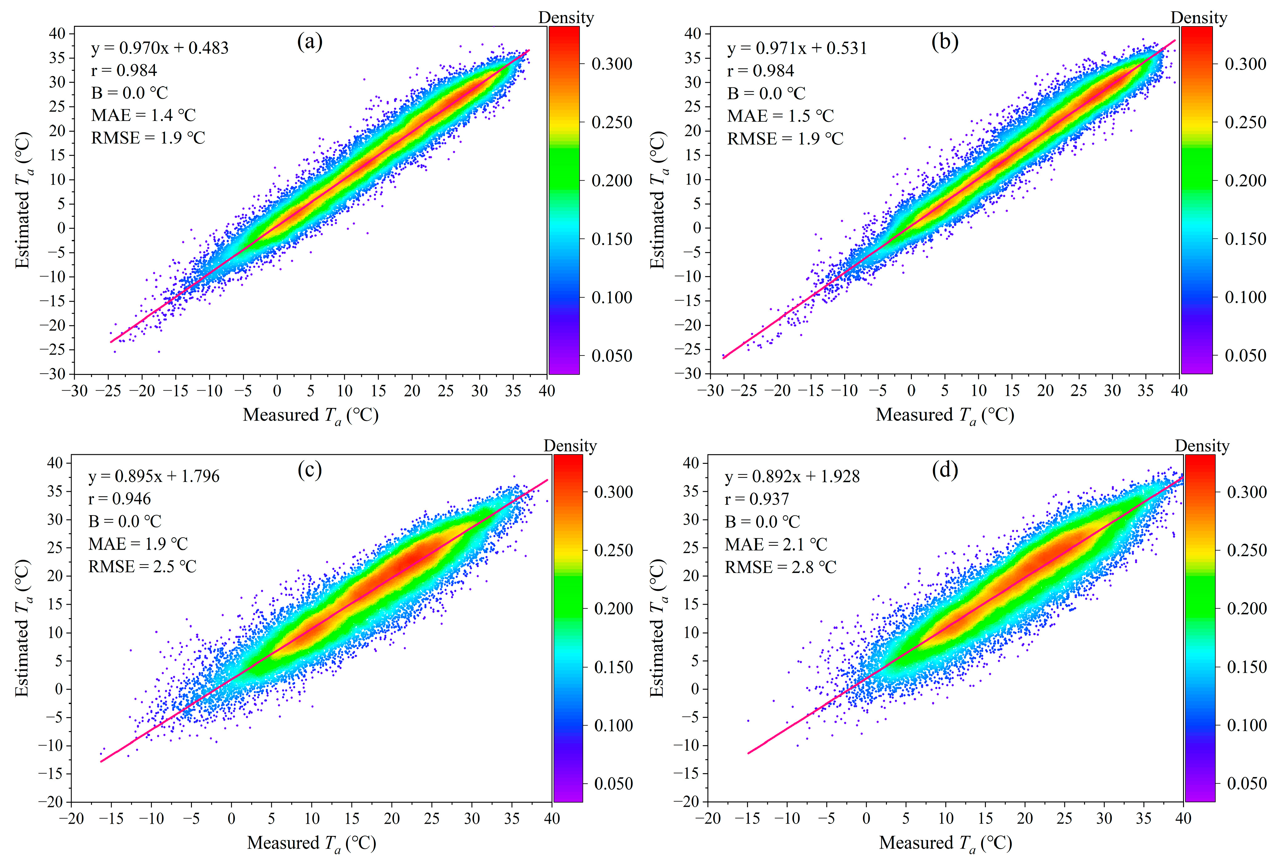
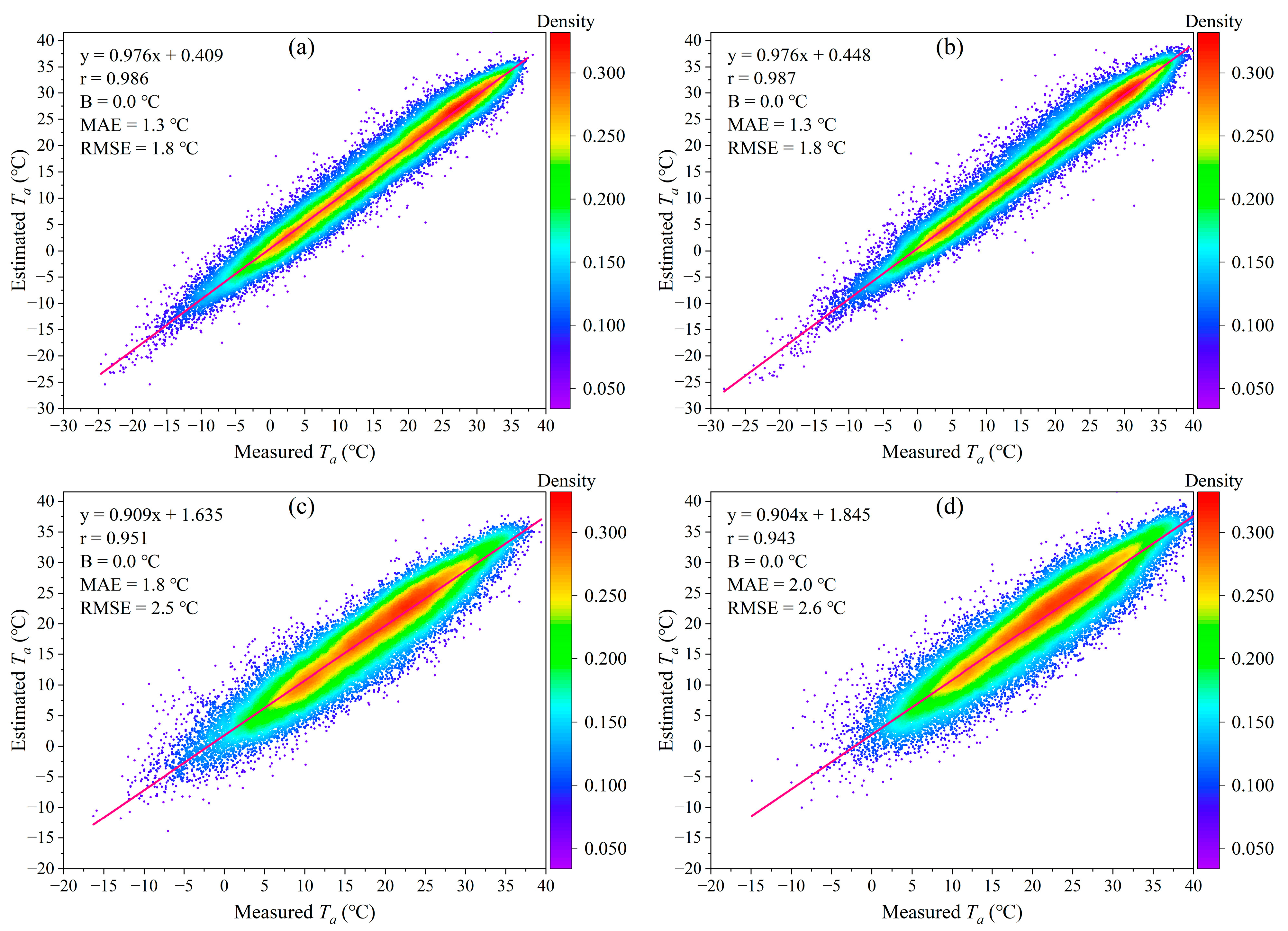
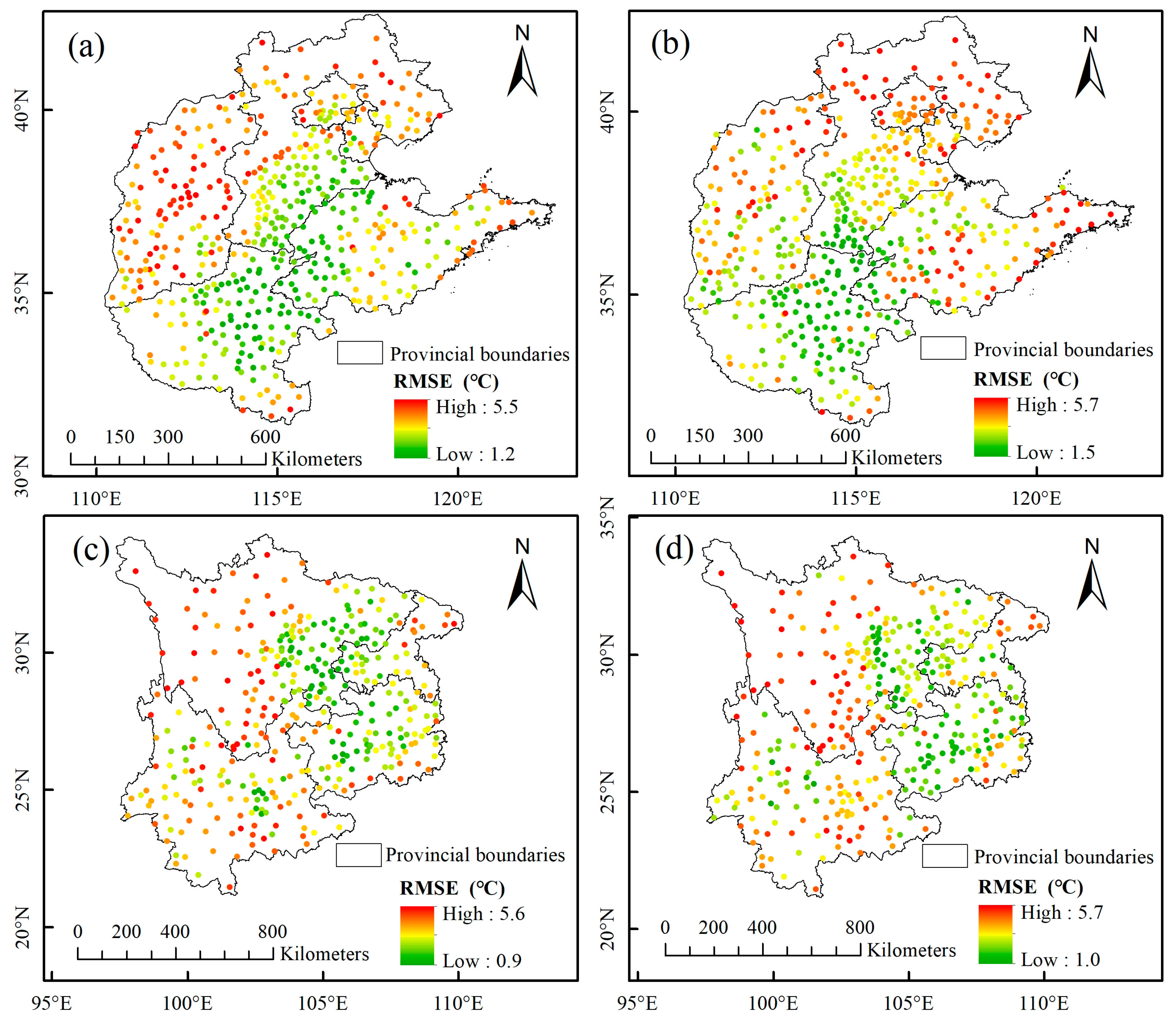
As in the case of $T_a$ under clear sky conditions, multiple stepwise linear regression was applied for the estimation of ${\mathrm{T}}_{\mathrm{a}}$ under cloudy sky conditions. The independent variables were LST (MOD06_L2/MYD06_L2), NDVI, SZA, and elevation. The actual observations were the dependent variables. Similarly, 70% of the samples were randomly selected to establish the multiple regression equation, and the remaining 30% of the samples were used for validation. The validation results are presented in Figure 3.

Compared with Table 5, it is clear that the multiple linear regression model produces better results for $T_a$ estimation than the simple linear regression model. The r values for the two regions were greater than 0.93, and the absolute values of B were less than 0.01 °C. The MAEs for the Terra and Aqua datasets of North China decreased by 2.2 and 1.1 °C, and the RMSEs were reduced by 2.6 and 1.4 °C, respectively. In Southwest China, the MAEs decreased by 1.5 and 0.6 °C, and the RMSEs decreased by 1.8 and 0.7 °C, respectively. In conclusion, the applicability of the multiple linear regression method to $T_a$ estimation is higher than a simple linear regression model under cloudy sky conditions. $T_a$ under cloudy sky conditions is not as accurate as under clear sky conditions, but all four statistics show that this is still acceptable given that the regression model for cloudy sky conditions does not involve atmospheric profile products. Furthermore, the LST under cloudy conditions may be subject to uncertainty due to varying cloud cover. The uncertainty of LST under cloudy sky conditions may lead to deviations in the coefficients corresponding to LST in the multiple regression model, resulting in errors in $T_a$ estimation.

4.3. Accuracy of Instantaneous $T_a$ Estimation under All-Weather Conditions

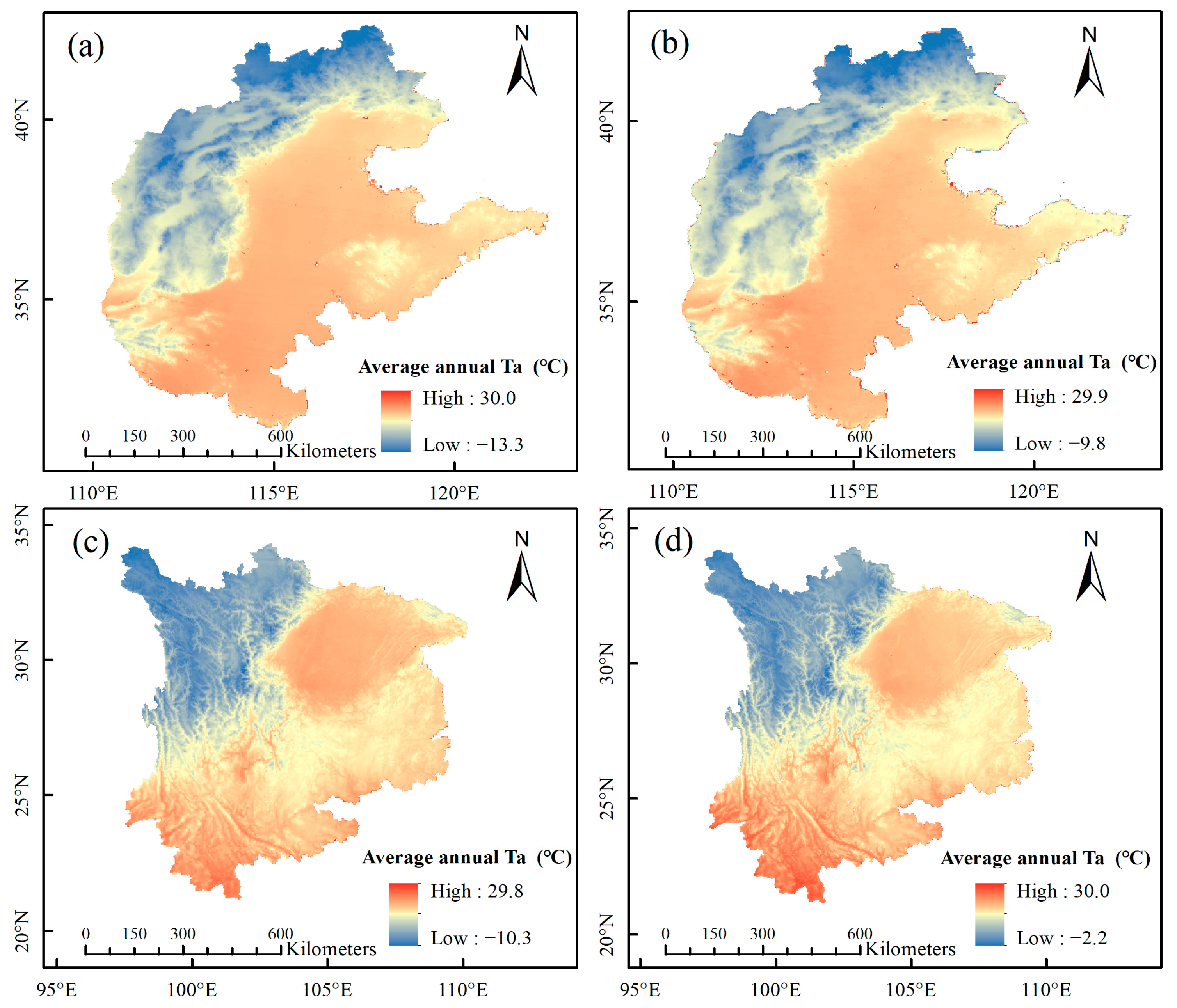
Based on the parameterization scheme described in Section 4.1 and Section 4.2, it is possible to obtain highly accurate instantaneous $T_a$ under all-weather conditions from the MODIS products, DEM, and observation datasets. The scatter diagram comparing estimated $T_a$ and measured $T_a$ in North and Southwest China is presented in Figure 4.

On the whole, the r, B, MAE, and RMSE calculated for North China through Terra and Aqua datasets were 0.986, 0.0 °C, 1.3 °C, 1.8 °C, and 0.987, 0.0 °C, 1.3 °C, and 1.8 °C, respectively; for Southwest China, they were 0.951, 0.0 °C, 1.8 °C, 2.5 °C, and 0.943, 0.0 °C, 2.0 °C, and 2.6 °C, respectively.

The discrepancy exists in $T_a$ estimation based on the MODIS Terra and Aqua datasets. The reason may be that the Terra and Aqua satellites operate in different orbits, resulting in different observation times and angles in the same area, so their solar zenith angles are different. As mentioned in Section 3.1, the influence of the SZA on $T_a$ is manifested in the total solar radiation reaching the ground, and the SZA is negatively correlated with the total solar radiation. Differences in total solar radiation may have contributed to major differences in $T_a$ estimates for the two datasets.

In order to further analyze the spatial uncertainty of the estimated $T_a$, the accuracy of the $T_a$ estimated by each meteorological station was calculated. Figure 5 shows the statistical metric RMSE of each meteorological station in North and Southwest China. Specifically, the RMSE at the meteorological station scale for North China is higher in the western and northern plateau regions and lower in the central plain regions. For Southwest China, the RMSE is higher in the plateau of the northwest region and lower in the basin and plain regions. Overall, compared with the spatial distribution of elevation in Figure 1, the $T_a$ estimation model performs better for meteorological stations located in plains and basins with lower elevations than those in plateaus with higher elevations. Complex terrain can reduce the correlation between $T_a$ and other variables, which may lead to model uncertainty in $T_a$ estimation.

The accuracy of instantaneous $T_a$ estimation varied somewhat with different land cover types. Therefore, the RMSEs of meteorological stations within each land cover type were demonstrated in the two study areas. Land cover types include cultivated land, woodland, grassland, and constructive land. The RMSEs of each land cover type are shown in

Table 7. RMSE of instantaneous $T_a$ estimation of land cover types (°C).

Study Area	Data Source	Cultivated Land	Woodland	Grassland	Constructive Land
North China	Terra	2.0	3.0	3.0	2.0
	Aqua	2.6	3.6	3.2	2.7
Southwest China	Terra	2.5	2.5	2.8	2.4
	Aqua	2.7	2.8	2.9	2.7

. For North China, the accuracy of $T_a$ estimation is ranked from high to low as cultivated land, constructive land, grassland, and woodland. The RMSEs for constructive land and construction land are relatively close, as are those for woodland and grassland. For Southwest China, the descending order of estimation accuracy is constructive land, cultivated land, woodland, and grassland. The accuracy difference between the four land cover types is not significant. In general, the estimation model exhibits better performance for stations situated in areas with constructive and cultivated land but displays relatively poor performance in regions characterized by woodland and grassland. Each land cover type corresponds to a different elevation, which is the main reason for differences in $T_a$ estimation. Specifically, for meteorological stations in North China, the average elevations of cultivated land, woodland, grassland, and constructive land are 300.63 m, 566.91 m, 841.10 m, and 227.20 m, respectively. In Southwest China, the average elevations for these land cover types are 1125.62 m, 1246.78 m, 1682.55 m, and 997.05 m, respectively. Woodland and grassland are primarily distributed in mountainous and hilly areas with higher elevations, while cultivated land and constructive land are largely influenced by human activities and mainly distributed in low-elevation plains and mountainous, hilly areas with lower elevations. In addition, cultivated land and construction land often have relatively simple land cover and uniform surface characteristics, resulting in higher estimation accuracy of $T_a$. There are variations in the precision of identical land cover types between the two study regions. In terms of woodland and grassland, the accuracy in Southwest China is higher than that in North China. Conversely, North China exhibits greater accuracy in estimating $T_a$ for cultivated and construction land, compared to Southwest China.

As mentioned in the introduction, most previous studies have focused on daily minimums and daily maximums or the average $T_a$ over a given period but rarely on the instantaneous $T_a$. The following two studies that used a similar method to estimate instantaneous $T_a$ are mentioned in this study. Based on the MODIS datasets, Xu et al. [60] took NDVI, water vapor pressure, surface albedo, and elevation as four influencing factors, used multiple regression analysis to fit the instantaneous $T_a$ under clear sky conditions. The RMSE of the estimation result is 2.3 °C; the accuracy is lower than that in this study. The estimation accuracy of $T_a$ is slightly different from that in Southwest China, but the RMSE difference with that in North China is more than 0.7 °C. Xu et al. [61] developed a statistical method for instantaneous $T_a$ using MODIS Aqua dataset and meteorological dataset. Four regression models with different independent variables resulted in MAE ranging from 2.2 to 2.3 °C. The estimation accuracy is slightly lower than that in this study (MAE ranges from 1.3 to 2.0 °C). Different from this study, the above two studies only involved the instantaneous $T_a$ under clear sky conditions but did not consider the instantaneous $T_a$ under cloudy sky conditions. In addition, the regression equations in this study were established on a daily scale, while the regression equations of the above two studies were the same for each day.

Our study demonstrates the feasibility of multiple stepwise regression models for $T_a$ estimation. However, there are several uncertainties associated with these models. Firstly, the variables selected for the multiple stepwise regression models were retrieved mainly from MODIS products, which may lead to varying results if the dataset changes. Secondly, the coefficient estimates in the multiple stepwise regression model are calculated based on the sample dataset, resulting in inherent errors and uncertainties. Thirdly, if the model exhibits multicollinearity, the prediction results may be uncertain. Additionally, if too many predictor variables are used in the multiple stepwise regression model, it may result in overfitting problems, which can negatively impact the models’ estimation accuracy. In order to mitigate these uncertainties, we performed quality control on the datasets, carefully selected features, and evaluated the model’s performance using various evaluation metrics.

4.4. Spatial Distribution of $T_a$ in North and Southwest China

The average annual $T_a$ under all-weather conditions was calculated. The spatial distribution of the average annual $T_a$ estimated with the Terra and Aqua datasets in North (Figure 6a,b) and Southwest China (Figure 6c,d) are presented. It should be especially emphasized that the average annual $T_a$ here represents the annual mean values of instantaneous $T_a$ at the time of satellite overpasses, which is somewhat different from the average annual $T_a$ in the traditional sense of meteorology.

The spatial distribution of $T_a$ is significantly influenced by altitude. Considering the spatial distribution of elevation in the study area (Figure 1), the $T_a$ values at high altitudes were significantly lower than those at low altitudes. Specifically, the overall distribution of the annual average $T_a$ in North China was higher in the south than the north, and in the east than the west. In Southwest China, the estimated $T_a$ showed a distribution where it was lower in the northwest than in the southeast. The annual average $T_a$ in the Sichuan Basin was significantly higher, while the western Sichuan Plain, which has a higher altitude, showed a lower $T_a$.

To illustrate the relationship between $T_a$ and elevation more accurately, the meteorological stations were divided into 17 zones in North China and 38 zones in Southwest China according to the elevation, with an initial elevation of 1 m and an interval of 100 m. Figure 7 presents the scatter plot of the estimated annual mean $T_a$ and its mean height for the elevation zones. To demonstrate the accuracy of the estimates, the $T_a$ observations at the meteorological stations were also introduced for comparison. The results display a significant negative correlation between elevation and $T_a$. The $T_a$ in Southwest China varies more than that in North China due to the elevation factor. In addition, even in the same elevation range, the $T_a$ in Southwest China is higher than that in North China due to climate and other natural factors.

5. Discussion

This study showed that the establishment of a multiple linear regression model is accurate in estimating $T_a$. However, the model’s performance is inadequate for small sample sizes. To ensure the stability of this model, the relationship between estimation accuracy and the sample size was analyzed. Meanwhile, the contribution of independent variables to $T_a$ estimation is different, the relative importance of them was expressed in this study to measure the effect of the independent variables on the dependent variable.

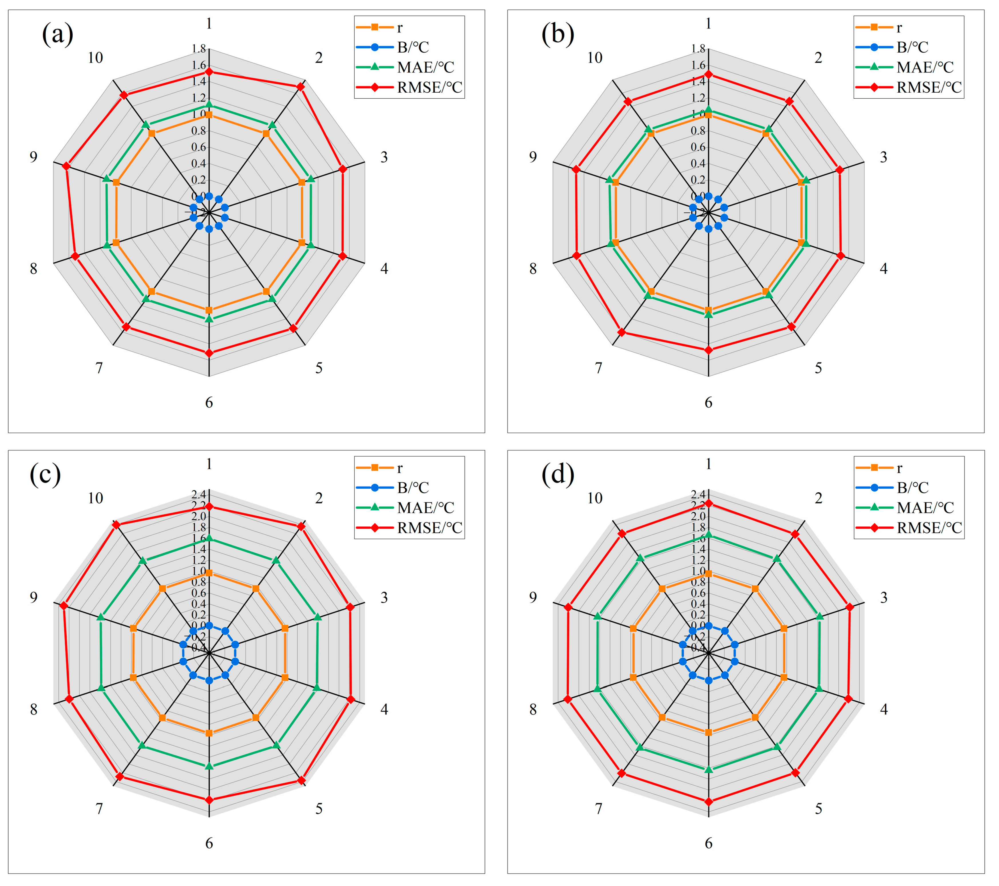
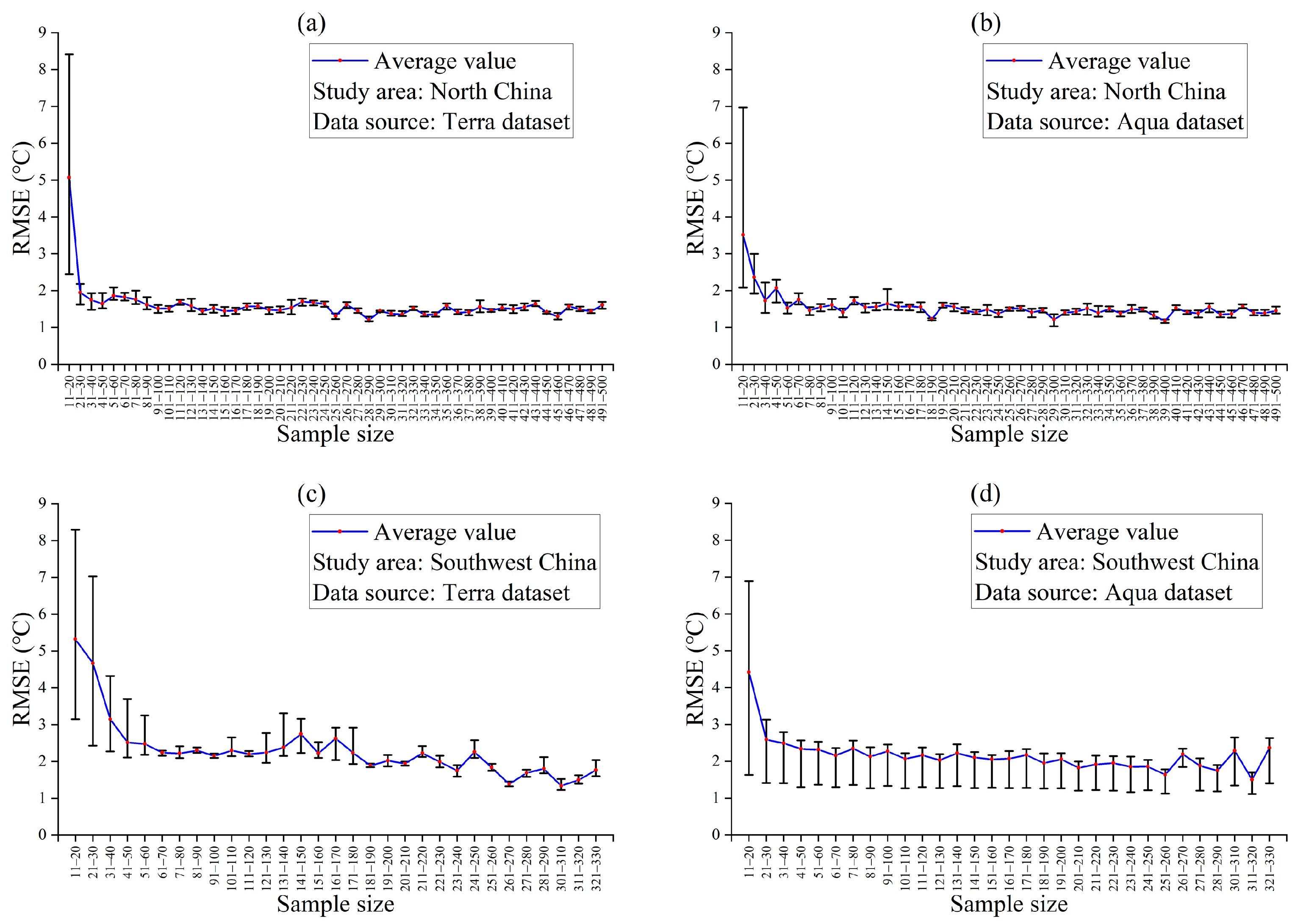
5.1. Effect of Sample Size on the Multiple Linear Regression Model

In the course of this study, there were some days with small sample sizes for estimating the instantaneous $T_a$ on clear days by the multiple stepwise linear regression method. This was mainly because MODIS atmospheric profile products only provide input information under clear sky conditions. In this vein, the applicability of linear regression is related to the sample size, as previously confirmed [62,63,64]. With limited sample information, the conclusions may be unreliable when the usual stepwise regression method is applied to analyze the effect of each explanatory variable x on the dependent variable y. To avoid the influence of a small sample size on the estimation results, the relationship between the statistical metric RMSE and the sample size was analyzed. Figure 8 shows the maximum, minimum, and average values of RMSE for the ten estimation results for each sample size. In addition, the sample size was divided into 49 groups in North China and 31 groups in Southwest China to analyze this relationship more accurately, with an initial number of 11 and an interval of 10.

According to the results, the RMSE of the model evaluation index was closer to the stable value with an increased sample size. The RMSEs tend to be 1.5 and 2.5 °C in North and Southwest China, respectively. In particular, the maximum, minimum, and average values of RMSE were significantly higher in the case of a sample size <30. Specifically, for sample size ranges between 11 and 20, the positive errors (difference between the maximum and average values) of RMSE for ten estimation results based on the MODIS Terra and Aqua datasets of North China were 3.3 and 3.5°C, respectively; the negative errors (absolute value of the difference between the minimum and the mean) were 2.6 and 1.4 °C, respectively. The positive errors of RMSE for Southwest China were 3.0 and 2.5 °C, while the negative errors were 2.2 and 2.8 °C, respectively. If the sample size ranges from 21 to 30, the positive errors of RMSE in North China were 0.6 and 0.2 °C, and the negative errors were 0.4 and 0.3 °C, respectively. The positive errors of RMSE in Southwest China were 2.4 °C and 0.5 °C, and the negative errors were 2.2 °C and 1.2 °C, respectively.

In summary, both positive and negative errors are significantly higher if the sample size ranges from 11 to 30. This indicates that the model is unstable in this case and potentially increases the overall error due to the randomness of the model itself. Therefore, the multiple regression equation was not established for a given day with a sample size <30 in this study.

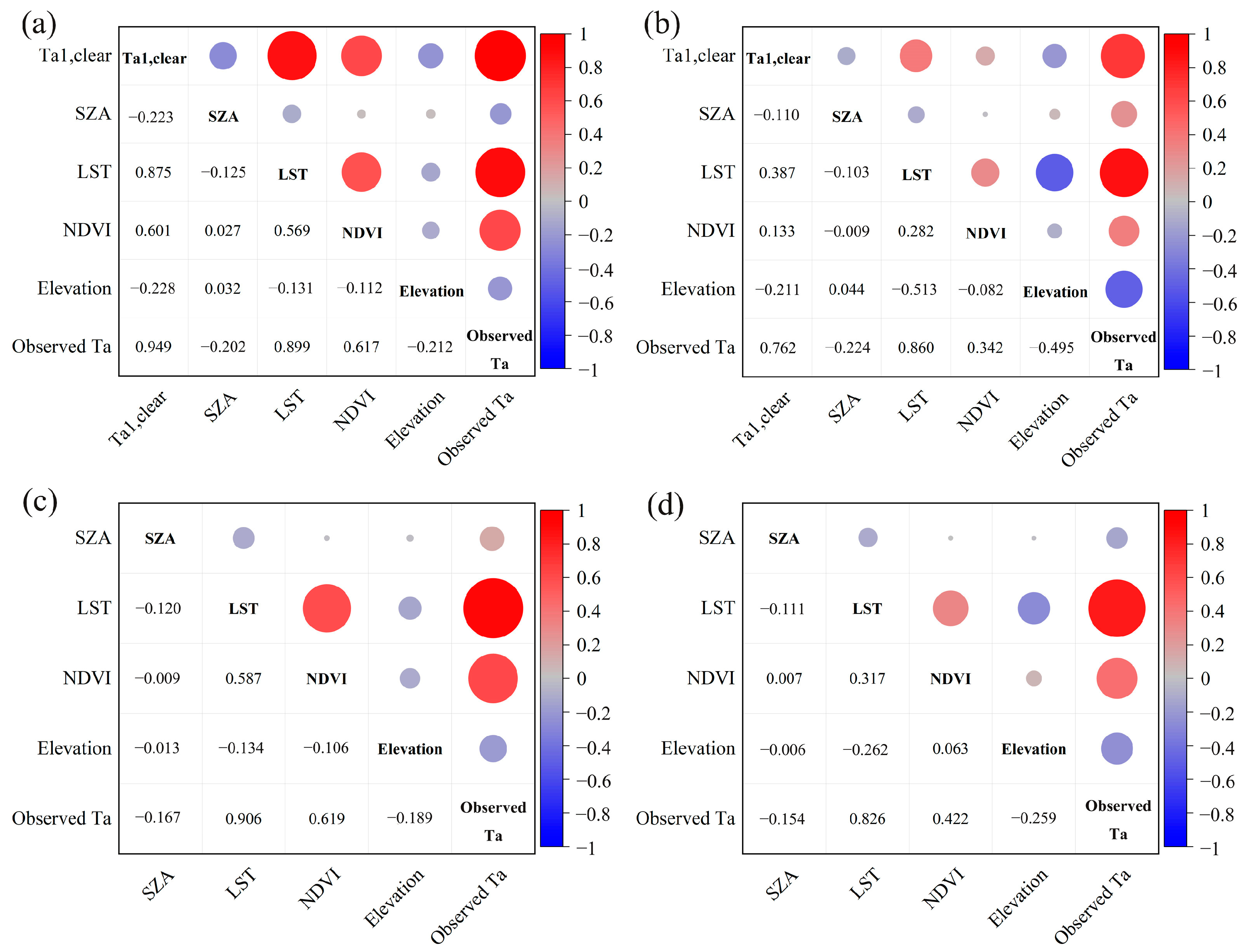
5.2. The Correlation of Variables and Relative Importance of Each Independent Variable

As mentioned in Section 3.1 and Section 3.2, $T_{a1,clear}$ (only for clear sky conditions), LST, NDVI, SZA, and elevation were selected as independent variables and observed $T_a$ was dependent variable. Stepwise regression was applied to construct multiple regression models. In order to explore the correlation of the variables, this study calculated the correlation coefficient of the variables. The value range of the correlation coefficient ranges from −1 to 1, and its absolute value is a measure that characterizes the correlation between two variables. The correlation results of each variable are shown in Figure 9. Specifically, the observed $T_a$ has a significant positive correlation with $T_{a1,clear}$, LST and NDVI, and a negative correlation with elevation and SZA.

Correlation analysis can indicate the close relationship between the dependent variable and $T_a$, but additional analysis is necessary to explain the degree to which each dependent variable contributes to $T_a$ estimation. To ensure comparability of the effects of different variables, the regression coefficient ${\beta }_i$ is typically transformed into a dimensionless standard regression coefficient [65], as shown in the following equation [66]:

$$b_i={\beta }_i\times \sigma \left(X_i\right) / \sigma \left(Y\right)$$

(10)

where ${\beta }_i$ is the regression coefficient of $X_i$, $b_i$ is the standardized regression coefficient of $X_i$, $\sigma \left(X_i\right),$ and $\sigma \left(Y\right)$ are the standard deviations of the independent variable $X_i$ and the dependent variable Y, respectively.

The standard regression coefficient eliminates the impact of the dimension of the variable $X_i$ and it is comparable. It could evaluate the relative significance of predictors, which represent the expected change in the response variable while keeping other predictors fixed [40]. The greater the absolute value of $b_i$, the more significant the contribution of its corresponding independent variable $X_i$ on Y. In order to intuitively compare the relative size of the standardized regression coefficients to measure the contribution degree of dependent variables to regression equations, the absolute value of $b_i$ under clear and cloudy sky conditions are shown in

Table 8. The $b_i$ of independent variables for clear and cloudy sky conditions.

Weather Conditions	Study Area	Data Source	${\mathit{T}}_{\mathit{a}1,\mathit{c}\mathit{l}\mathit{e}\mathit{a}\mathit{r}}$	LST	SZA	NDVI	Elevation
Clear sky conditions	NorthChina	Terra	0.296	0.232	0.200	0.044	0.551
		Aqua	0.304	0.172	0.242	0.068	0.617
	Southwest China	Terra	0.339	0.149	0.155	0.066	0.656
		Aqua	0.321	0.160	0.257	0.087	0.694
Cloudy sky conditions	NorthChina	Terra	-	0.438	0.193	0.067	0.492
		Aqua	-	0.512	0.189	0.066	0.427
	Southwest China	Terra	-	0.361	0.248	0.105	0.536
		Aqua	-	0.517	0.320	0.079	0.484

. It should be noted that since the regression equation in this study was established on a daily scale, the average of the absolute values of $b_i$ for each independent variable of all regression equations was calculated.

The contribution of five independent variables based on the Terra dataset to $T_a$ estimation under clear sky conditions in North China is elevation, $T_{a1,clear}$, LST, SZA, and NDVI in descending order. For other clear sky conditions, the contribution of independent variables in descending order is elevation, $T_{a1,clear}$, SZA, LST, and NDVI. Specifically, the contribution of independent variables $T_{a1,clear}$, elevation, and NDVI in Southwest China to $T_a$ estimation is greater than that in North China, while the LST contributes more in North China than in Southwest China. Under cloudy sky conditions, the overall contribution of four independent variables from the Terra and Aqua dataset, in descending order, are elevation, LST, SZA, and NDVI, and LST, elevation, SZA, and NDVI, respectively. Moreover, the contribution of elevation, SZA, and NDVI in Southwest China is greater than those in North China, and the contribution of LST in North China is higher than that in Southwest China.

On the whole, the elevation contributes the most and has the greatest impact on $T_a$ estimation. The influence of elevation on $T_a$ is reflected in the fact that as the altitude increases, atmospheric pressure decreases, leading to a decrease in air density and, thus a decrease in $T_{a }$ [67]. The contribution degree of elevation in Southwest China is greater than that in North China. Therefore, the difference in topographical conditions may be one of the influencing factors for the difference in $T_a$ estimation in the two study regions. It is followed by LST, $T_{a1,clear}$, and SZA. NDVI has relatively little influence on $T_a$ estimation compared with other independent variables, and its contribution degree in Southwest China is greater than that in North China. In conclusion, the independent variables contribute differently to $T_a$ estimates in the two study regions, which may lead to differences in $T_a$ estimation of them.

6. Conclusions

The instantaneous $T_a$ was estimated under clear and cloudy sky conditions from 2016 to 2017 in North and Southwest China based on MODIS products provided by the Terra and Aqua satellites, actual $T_a$ observations and DEM datasets. In particular, this study focused on the application of MODIS atmospheric profile products in $T_a$ estimation. Moreover, the accuracy of different approaches was examined.

Under clear sky conditions, the $T_a$ estimates obtained by the atmospheric profile extrapolation and average methods had a strong correlation with the $T_a$ observations (r ranging from 0.758 to 0.969). However, the accuracy of these two estimation methods was poor, with RMSE ranging from 3.5 to 5.2 °C for North China and from 4.0 to 7.7 °C for Southwest China. If the $T_a$ obtained by the atmospheric profile extrapolation method is significantly underestimated; the average method can minimize the underestimation and achieve higher accuracy. The accuracy of the $T_a$ estimates under clear sky conditions obtained with the multiple linear regression model were significantly improved by introducing auxiliary data. The average RMSEs of $T_a$ estimated using the Terra and Aqua datasets in North China were reduced by 1.9 and 2.4 °C, respectively, compared with the minimum RMSEs of the previous two methods. Similarly, the RMSEs in Southwest China decreased by 1.8 and 2.2 °C, respectively. The multiple stepwise regression method is also well-suited for use under cloudy sky conditions, with RMSE of 1.9 for both the Terra and Aqua datasets in North China and RMSEs of 2.5 and 2.8 °C in Southwest China. For all estimation models based on the two types of datasets in the two study regions, $T_a$ accuracy estimated under cloudy sky conditions is lower than that under clear sky conditions. The reason for this phenomenon might be related to the uncertainty of LST under cloudy sky conditions due to the influence of different cloud cover. Therefore, the following methods are used to reduce the uncertainty of LST: other related variables are added as independent variables to assist in the prediction of $T_a$; the accuracy and stability of the model are evaluated by cross-validation to ensure the reliability of the model. Furthermore, the MAEs and RMSEs under all-weather conditions calculated for North China were both 1.3 °C and 1.8 °C, while for Southwest China, they were 1.8, 2.0 °C, and 2.5, 2.6 °C, respectively.

The accuracy of instantaneous $T_a$ estimation is influenced by complex factors. The results of the study show that the estimation model in this study has high applicability in two regions with different geomorphological and climatic conditions. Specifically, the $T_a$ estimation model performs better for meteorological stations located in plains and basins with lower elevations compared to those in plateaus with higher elevations. Among all the independent variables, elevation has the greatest impact on $T_a$ estimation. The contribution degree of elevation in Southwest China is greater than in North China. It performs well for stations located in constructive land and cultivated land and performs poorly in woodland and grassland areas. In addition, the accuracy of $T_a$ estimation is not identical if the input datasets are from different satellites with different overpass times. For Southwest China, the accuracy of $T_a$ estimated by the Terra dataset is higher than that of the Aqua dataset, while the opposite is true in North China.

References

1. Wang, C.; Bi, X.; Luan, Q.; Li, Z. Estimation of Daily and Instantaneous Near-Surface Air Temperature from MODIS Data Using Machine Learning Methods in the Jingjinji Area of China. Remote Sens. 2022, 14, 1916. [Google Scholar] [CrossRef]
2. Nieto, H.; Sandholt, I.; Aguado, I.; Chuvieco, E.; Stisen, S. Air temperature estimation with MSG-SEVIRI data: Calibration and validation of the TVX algorithm for the Iberian Peninsula. Remote Sens. Environ. 2011, 115, 107–116. [Google Scholar] [CrossRef]
3. Lofgren, B.M.; Hunter, T.S.; Wilbarger, J. Effects of using air temperature as a proxy for potential evapotranspiration in climate change scenarios of Great Lakes basin hydrology. Great Lakes Res. 2011, 37, 744–752. [Google Scholar] [CrossRef]
4. Harvell, C.D.; Mitchell, C.E.; Ward, J.R.; Altizer, S.; Dobson, A.P.; Ostfeld, R.S.; Samuel, M.D. Climate warming and disease risks for terrestrial and marine biota (Review). Science 2002, 296, 2158–2162. [Google Scholar] [CrossRef]
5. Westerling, A.L.; Hidalgo, H.G.; Cayan, D.R.; Swetnam, T.W. Warming and Earlier Spring Increase Western U.S. Forest Wildfire Activity. Science 2006, 313, 940–943. [Google Scholar] [CrossRef]
6. Yoo, C.; Im, J.; Park, S.; Quackenbush, L.J. Estimation of daily maximum and minimum air temperatures in urban landscapes using MODIS time series satellite data. ISPRS-J. Photogramm. Remote Sens. 2018, 137, 149–162. [Google Scholar] [CrossRef]
7. Shamir, E.; Georgakakos, K.P. MODIS Land Surface Temperature as an Index of Surface Air Temperature for Operational Snowpack Estimation. Remote Sens. Environ. 2014, 152, 83–98. [Google Scholar] [CrossRef]
8. Vancutsem, C.; Ceccato, P.; Dinku, T.; Connor, S.J. Evaluation of MODIS land surface temperature data to estimate air temperature in different ecosystems over Africa. Remote Sens. Environ. 2010, 114, 449–465. [Google Scholar] [CrossRef]
9. Asplin, M.G.; Floyer, J.A.; McKendry, I.G.; Moore, R.D.; Stahl, K. Comparison of approaches for spatial interpolation of daily air temperature in a large region with complex topography and highly variable station density. Agric. For. Meteorol. 2006, 139, 224–236. [Google Scholar]
10. Wloczyk, C.; Borg, E.; Richter, R.; Miegel, K. Estimation of instantaneous air temperature above vegetation and soil surfaces from Landsat 7 ETM+ data in northern Germany. Int. J. Remote Sens. 2011, 32, 9119–9136. [Google Scholar] [CrossRef]
11. Williamson, S.N.; Hik, D.S.; Gamon, J.A.; Kavanaugh, J.L.; Flowers, G.E. Estimating Temperature Fields from MODIS Land Surface Temperature and Air Temperature Observations in a Sub-Arctic Alpine Environment. Remote Sens. 2014, 6, 946–963. [Google Scholar] [CrossRef]
12. Kloog, I.; Chudnovsky, A.; Koutrakis, P.; Schwartz, J. Temporal and spatial assessments of minimum air temperature using satellite surface temperature measurements in Massachusetts, USA. Remote Sens. Environ. 2012, 432, 85–92. [Google Scholar] [CrossRef] [PubMed]
13. Czakowski, K.P.; Goward, S.N. Thermal Remote Sensing of Near Surface Environmental Variables: Application Over the Oklahoma. Prof. Geogr. 2000, 52, 345. [Google Scholar] [CrossRef]
14. Prihodko, L.; Goward, S.N. Estimation of air temperature from remotely sensed surface observations. Remote Sens. Environ. 1997, 60, 335–346. [Google Scholar] [CrossRef]
15. Zhu, W.; Lu, A.; Jia, S. Estimation of daily maximum and minimum air temperature using MODIS land surface temperature products. Remote Sens. Environ. 2013, 130, 62–73. [Google Scholar] [CrossRef]
16. Sun, L.; Sun, R.; Li, X.; Liang, S.; Zhang, R. Monitoring surface soil moisture status based on remotely sensed surface temperature and vegetation index information. Agric. For. Meteorol. 2012, 166–167, 175–187. [Google Scholar] [CrossRef]
17. Zhang, R.; Rong, Y.; Tian, J.; Su, H.; Li, Z.; Liu, S. A Remote Sensing Method for Estimating Surface Air Temperature and Surface Vapor Pressure on a Regional Scale. Remote Sens. 2015, 7, 6005–6025. [Google Scholar] [CrossRef]
18. Pape, R.; Lffler, J. Modelling spatio-temporal near-surface temperature variation in high mountain landscapes. Ecol. Model. 2004, 178, 483–501. [Google Scholar] [CrossRef]
19. Bhati, S.; Mohan, M. WRF model evaluation for the urban heat island assessment under varying land use/land cover and reference site conditions. Theor. Appl. Climatol. 2016, 126, 385–400. [Google Scholar] [CrossRef]
20. Chen, F.; Yang, X.; Zhu, W. WRF simulations of urban heat island under hot-weather synoptic conditions: The case study of Hangzhou City, China. Atmos. Res. 2014, 138, 364–377. [Google Scholar] [CrossRef]
21. Noi, P.T.; Kappas, M.; Degener, J. Estimating Daily Maximum and Minimum Land Air Surface Temperature Using MODIS Land Surface Temperature Data and Ground Truth Data in Northern Vietnam. Remote Sens. 2016, 8, 1002. [Google Scholar] [CrossRef]
22. Benali, A.; Carvalho, A.C.; Nunes, J.P.; Carvalhais, N.; Santos, A. Estimating Air Surface Temperature in Portugal Using MODIS Lst Data. Remote Sens. Environ. 2012, 124, 108–121. [Google Scholar] [CrossRef]
23. Janatian, N.; Sadeghi, M.; Sanaeinejad, S.H.; Bakhshian, E.; Farid, A.; Hasheminia, S.M.; Ghazanfari, S. A statistical framework for estimating air temperature using MODIS land surface temperature data. Int. J. Climatol. 2017, 37, 1181–1194. [Google Scholar] [CrossRef]
24. Hrisko, J.; Ramamurthy, P.; Yu, Y.Y.; Yu, P.; Melecio-Vazquez, D. Urban air temperature model using GOES-16 LST and a diurnal regressive neural network algorithm. Remote Sens. Environ. 2020, 237, 111495. [Google Scholar] [CrossRef]
25. Ruiz-Álvarez, M.; Alonso-Sarria, F.; Gomariz-Castillo, F. Interpolation of instantaneous air temperature using geographical and MODIS derived variables with machine learning techniques. ISPRS Int. J. Geo Inf. 2019, 8, 382. [Google Scholar] [CrossRef]
26. Yao, R.; Wang, L.C.; Huang, X.; Li, L.; Sun, J.; Wu, X.J.; Jiang, W.X. Developing a temporally accurate air temperature dataset for Mainland China. Sci. Total Environ. 2020, 706, 136037. [Google Scholar] [CrossRef]
27. Peón, J.; Recondo, C.; Calleja, J.F. Improvements in the estimation of daily minimum air temperature in peninsular Spain using MODIS land surface temperature. Int. J. Remote Sens. 2014, 35, 5148–5166. [Google Scholar] [CrossRef]
28. Recondo, C.; Corbea-Pérez, A.; Peón, J.; Pendás, E.; Ramos, M.; Calleja, J.F.; Pablo, M.Á.d.; Fernández, S.; Corrales, J.A. Empirical Models for Estimating Air Temperature Using MODIS Land Surface Temperature (and Spatiotemporal Variables) in the Hurd Peninsula of Livingston Island, Antarctica, between 2000 and 2016. Remote Sens. 2022, 14, 3206. [Google Scholar] [CrossRef]
29. Bisht, G.; Bras, R.L. Estimation of net radiation from the MODIS data under all sky conditions: Southern Great Plains case study. Remote Sens. Environ. 2010, 114, 1522–1534. [Google Scholar] [CrossRef]
30. Jocik, A.M. Estimate Ambient Air Temperature at Regional Level Using Remote Sensing Techniques. Master’s Thesis, International Institute for Geo-Information Science and Earth Observation (ITC), Enschede, The Netherlands, 2004. [Google Scholar]
31. Zhu, W.; Lu, A.; Jia, S.; Yan, J.; Mahmood, R. Retrievals of all-weather daytime air temperature from MODIS products. Remote Sens. Environ. 2017, 189, 152–163. [Google Scholar] [CrossRef]
32. Zhang, W.; Zhang, B.; Zhu, W.; Tang, X.; Li, F.; Liu, X.; Yu, Q. Comprehensive assessment of MODIS-derived near-surface air temperature using wide elevation-spanned measurements in China. Sci. Total Environ. 2021, 800, 149535. [Google Scholar] [CrossRef] [PubMed]
33. Shi, L.; Liu, P.; Kloog, I.; Lee, M.; Kosheleva, A.; Schwartz, J. Estimating daily air temperature across the Southeastern United States using high-resolution satellite data: A statistical modeling study. Environ Res. 2016, 146, 51–58. [Google Scholar] [CrossRef] [PubMed]
34. Shen, S.; Leptoukh, G.G. Estimation of surface air temperature over central and eastern Eurasia from MODIS land surface temperature. Environ. Res. Lett. 2011, 6, 045206. [Google Scholar] [CrossRef]
35. Xu, Y.; Knudby, A.; Ho, H. Estimating daily maximum air temperature from MODIS in British Columbia, Canada. Int. J. Remote Sens. 2014, 35, 8108–8121. [Google Scholar] [CrossRef]
36. Meyer, H.; Katurji, M.; Appelhans, T.; Müller, M.U.; Nauss, T.; Roudier, P.; Zawar-Reza, P. Mapping Daily Air Temperature for Antarctica Based on MODIS LST. Remote Sens. 2016, 8, 732. [Google Scholar] [CrossRef]
37. Garcia, M.; Fernández, N.; Villagarcía, L.; Domingo, F.; Puigdefábregas, J.; Sandholt, I. Accuracy of the Temperature–Vegetation Dryness Index using MODIS under water-limited vs. energy-limited evapotranspiration conditions. Remote Sens. Environ. 2014, 149, 100–117. [Google Scholar] [CrossRef]
38. Bisht, G.; Venturini, V.; Islam, S.; Jiang, L. Estimation of the net radiation using MODIS (Moderate Resolution Imaging Spectroradiometer) data for clear sky days. Remote Sens. Environ. 2005, 97, 52–67. [Google Scholar] [CrossRef]
39. Zhao, S.; Yang, Y.; Qiu, G.; Qin, Q.; Yao, Y.; Xiong, Y.; Li, C. Remote detection of bare soil moisture using a surface-temperature-based soil evaporation transfer coefficient. Int. J. Appl. Earth Obs. 2010, 12, 351–358. [Google Scholar] [CrossRef]
40. Yang, Y.; Cai, W.; Yang, J. Evaluation of MODIS Land Surface Temperature Data to Estimate Near-Surface Air Temperature in Northeast China. Remote Sens. 2017, 9, 410. [Google Scholar] [CrossRef]
41. Bai, H.; Gong, Z.; Sun, G.; Li, L.; Zhou, L. Influence of Meteorological Elements on Summer Vegetation Coverage in North China. Chin. J. Atmos. Sci. 2022, 46, 27–39. (In Chinese) [Google Scholar]
42. Huang, Y.; Wang, H. Is the Regional Precipitation Predictable in Decadal Scale? A Possible Approach for the Decadal Prediction of the Summer Precipitation Over North China. Earth. Space Sci. 2020, 7, e2019EA000986. [Google Scholar] [CrossRef]
43. Song, C.; Huang, X.; Les, O.; Ma, H.; Liu, R. The Economic Impact of Climate Change on Wheat and Maize Yields in the North China Plain. Int. J. Environ. Res. Public Health 2022, 19, 5707. [Google Scholar] [CrossRef] [PubMed]
44. Wu, J.; Cheng, G.; Wang, N.; Shen, H.; Ma, X. Spatiotemporal Patterns of Multiscale Drought and Its Impact on Winter Wheat Yield over North China Plain. Agronomy 2022, 12, 1209. [Google Scholar] [CrossRef]
45. Zheng, G.; Li, Y.; Chen, Q.; Zhou, X.; Gao, G.; Li, M.; Duan, T. The increasing predominance of extreme precipitation in Southwest China since the late 1970s. Atmos. Ocean. Sci. Lett. 2022, 15, 45–50. [Google Scholar] [CrossRef]
46. Sun, H.; Wang, X.; Fan, D.; Sun, O.J. Contrasting vegetation response to climate change between two monsoon regions in Southwest China: The roles of climate condition and vegetation height. Sci. Total Environ. 2022, 802, 149643. [Google Scholar] [CrossRef]
47. Pei, J.; Niu, Z.; Wang, L.; Huang, N.; Cao, J. Quantifying the spatio-temporal variations and impact factors for vegetation coverage in the karst regions of Southwest China using Landsat data and Google Earth engine. Proc. SPIE 2018, 10780, 107800E. [Google Scholar]
48. Huang, F.; Zhan, W.; Wang, Z.-H.; Voogt, J.; Hu, L.; Quan, J.; Liu, C.; Zhang, N.; Lai, J. Satellite identification of atmospheric-surface-subsurface urban heat islands under clear sky. Remote Sens. Environ. 2020, 250, 112039. [Google Scholar] [CrossRef]
49. Seddon, A.W.R.; Macias-Fauria, M.; Long, P.R.; Benz, D.; Willis, K.J. Sensitivity of global terrestrial ecosystems to climate variability. Nature 2016, 531, 229–232. [Google Scholar] [CrossRef]
50. Orellana-Samaniego, M.L.; Ballari, D.; Guzman, P.; Ospina, J.E. Estimating monthly air temperature using remote sensing on a region with highly variable topography and scarce monitoring in the southern Ecuadorian Andes. Theor. Appl. Climatol. 2021, 144, 949–966. [Google Scholar] [CrossRef]
51. Huang, R.; Zhang, C.; Huang, J.; Zhu, D.; Wang, L.; Liu, J. Mapping of Daily Mean Air Temperature in Agricultural Regions Using Daytime and Nighttime Land Surface Temperatures Derived from TERRA and AQUA MODIS Data. Remote Sens. Environ. 2015, 7, 8728–8756. [Google Scholar] [CrossRef]
52. Noi, P.T.; Degener, J.; Kappas, M. Comparison of Multiple Linear Regression, Cubist Regression, and Random Forest Algorithms to Estimate Daily Air Surface Temperature from Dynamic Combinations of MODIS LST Data. Remote Sens. 2017, 9, 398. [Google Scholar] [CrossRef]
53. Bappa, S.A.; Malaker, T.; Mia, M.R.; Islam, M.D. Spatio-temporal variation of land use and land cover changes and their impact on land surface temperature: A case of Kutupalong Refugee Camp, Bangladesh. Heliyon 2022, 8, e10449. [Google Scholar] [CrossRef] [PubMed]
54. Zakšek, K.; Schroedter-Homscheidt, M. Parameterization of air temperature in high temporal and spatial resolution from a combination of the SEVIRI and MODIS instruments. ISPRS-J. Photogramm. Remote Sens. 2009, 64, 414–421. [Google Scholar] [CrossRef]
55. Kankeo, D.; Hind, M. Relation between NDVI and Maximum Air Temperature on Clear DaysCertification of the Estimation Method using NDVI for Vegetation Mitigation Effects on Air Temperature. J. Jpn. Soc. Hydrol. Water Resour. 1996, 9, 271–279. [Google Scholar] [CrossRef]
56. Cresswell, M.P.; Morse, A.P.; Thomson, M.C.; Connor, S.J. Estimating surface air temperatures, from Meteosat land surface temperatures, using an empirical solar zenith angle model. Int. J. Remote Sens. 1999, 20, 1125–1132. [Google Scholar] [CrossRef]
57. Wang, R.; Yao, X.; Shi, Y.; Wu, C.; Liu, B. Study on air temperature estimation and its influencing factors in a complex mountainous area. PLoS ONE 2022, 17, e0272946. [Google Scholar]
58. Stisen, S.; Sandholt, I.; Nørgaard, A.; Fensholt, R.; Eklundh, L. Estimation of diurnal air temperature using MSG SEVIRI data in West Africa. Remote Sens. Environ. 2007, 110, 262–274. [Google Scholar] [CrossRef]
59. Jia, S.; Zhu, W.; Lu, A.; Yan, T. A statistical spatial downscaling algorithm of TRMM precipitation based on NDVI and DEM in the Qaidam Basin of China. Remote Sens. Environ. 2011, 115, 3069–3079. [Google Scholar] [CrossRef]
60. Xu, W.; Sun, R.; Jin, Z.; Hu, B. Estimation of near surface air temperature based on MODIS data. Meteorol. Environ. Sci. 2015, 38, 1–6. (In Chinese) [Google Scholar]
61. Xu, Y.; Qin, Z.; Shen, Y. Study on the estimation of near-surface air temperature from MODIS data by statistical methods. Int. J. Remote Sens. 2012, 33, 7629–7643. [Google Scholar] [CrossRef]
62. Hanley, J.A. Simple and multiple linear regression: Sample size considerations (Article). J. Clin. Epid. 2016, 79, 112–119. [Google Scholar] [CrossRef] [PubMed]
63. Jan, S.-L.; Shieh, G. Sample size calculations for model validation in linear regression analysis. BMC Med. Res. Method 2019, 19, 54. [Google Scholar] [CrossRef] [PubMed]
64. Kovács, D.; Király, P.; Tóth, G. Sample-size dependence of validation parameters in linear regression models and in QSAR. SAR QSAR Environ. Res. 2021, 32, 247–268. [Google Scholar] [CrossRef]
65. Mayer, L.; Younger, M. Estimation of Standardized Regression Coefficients. J. Amer. Stat. Assoc. 1976, 71, 154. [Google Scholar] [CrossRef]
66. Liu, S. The Contributory Big or Small of Every Variability to Regression Analyse and Realize in Multivariable Regression. J. Math. Med. 2005, 18, 524–525. (In Chinese) [Google Scholar]
67. Barry, R.G. Mountain Weather and Climate; Cambridge University Press: New York, NY, USA, 2008. [Google Scholar]
Figure 1. Geographic location of the study areas and distribution of meteorological stations.
Remotesensing 15 02701 g001
Figure 2. Accuracy of ten instantaneous T a estimations obtained with multiple linear regression model ( T a 3 , c l e a r ): (a) North China, Terra dataset; (b) North China, Aqua dataset; (c) Southwest China, Terra dataset; (d) Southwest China, Aqua dataset.
Remotesensing 15 02701 g002
Figure 3. Accuracy of instantaneous T a estimation under cloudy sky conditions produced by multiple linear regression model ( T a 3 , c l o u d y ): (a) North China, Terra dataset; (b) North China, Aqua dataset; (c) Southwest China, Terra dataset; (d) Southwest China, Aqua dataset.
Remotesensing 15 02701 g003
Figure 4. Accuracy of instantaneous T a estimation under all-weather conditions: (a) North China, Terra data; (b) North China, Aqua dataset; (c) Southwest China, Terra dataset; (d) Southwest China, Aqua dataset.
Remotesensing 15 02701 g004
Figure 5. RMSE of instantaneous T a estimation meteorological stations: (a) North China, Terra dataset; (b) North China, Aqua dataset; (c) Southwest China, Terra dataset; (d) Southwest China, Aqua dataset.
Remotesensing 15 02701 g005
Figure 6. Spatial distribution of average annual T a estimation from 2016 to 2017: (a) North China, Terra dataset; (b) North China, Aqua dataset; (c) Southwest China, Terra dataset; (d) Southwest China, Aqua dataset.
Remotesensing 15 02701 g006
Figure 7. Scatter plot between observed (red dots), estimated (blue dots) T a and elevation: (a) North China, Terra dataset; (b) North China, Aqua dataset; (c) Southwest China, Terra dataset; (d) Southwest China, Aqua dataset.
Remotesensing 15 02701 g007
Figure 8. Relationship between sample size and RMSE of T a estimation: (a) North China, Terra dataset; (b) North China, Aqua dataset; (c) Southwest China, Terra dataset; (d) Southwest China, Aqua dataset.
Remotesensing 15 02701 g008
Figure 9. The correlation between each variable and T a : (a) North China, clear sky conditions; (b) Southwest China, clear sky conditions; (c) North China, cloudy sky conditions; (d) Southwest, cloudy sky conditions.
Remotesensing 15 02701 g009