
Improving the Spatial Accuracy of UAV Platforms Using Direct Georeferencing Methods: An Application for Steep Slopes


Abstract
:
1. Introduction
2. Materials and Methods
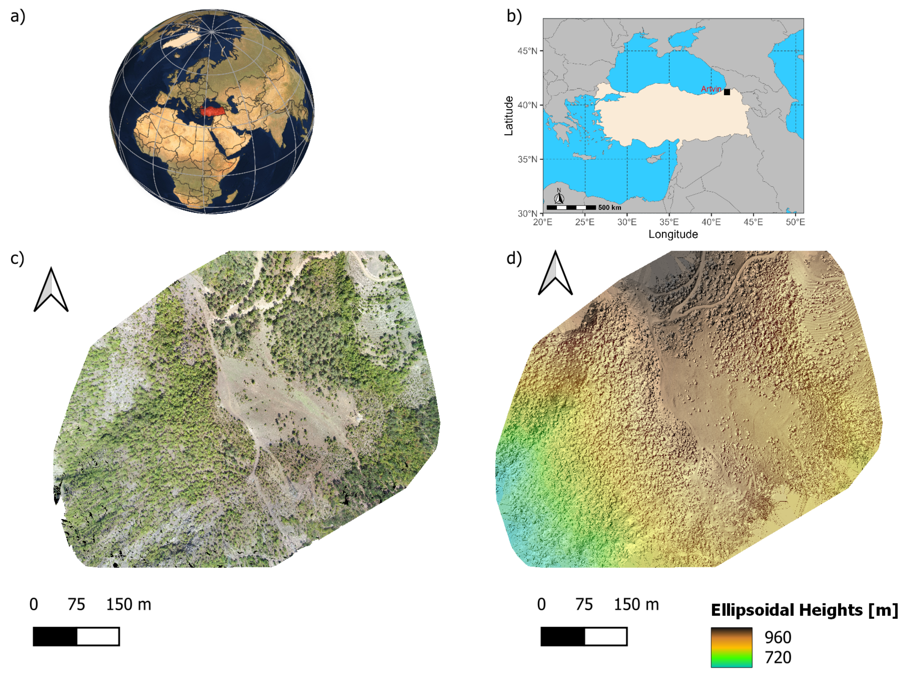
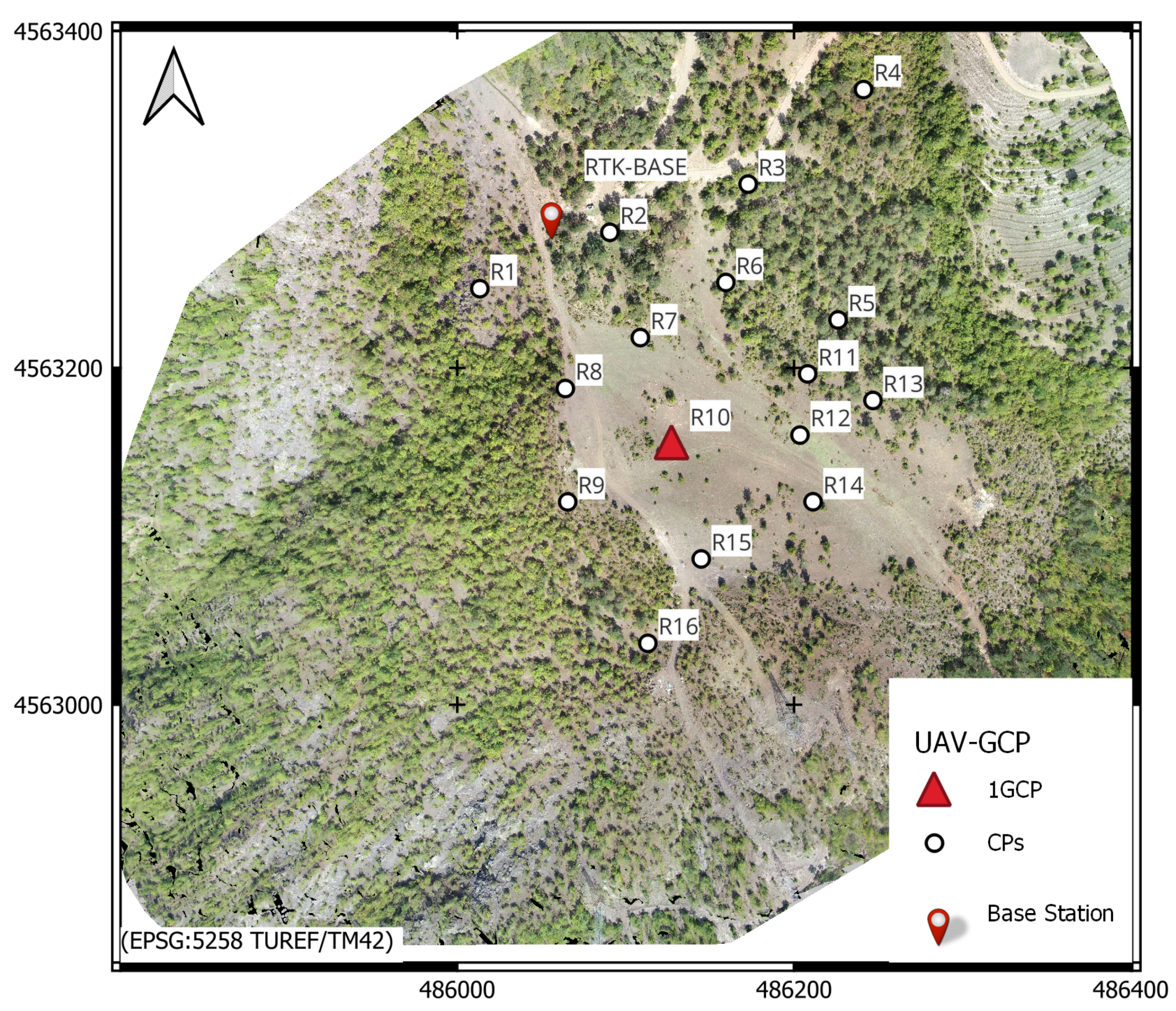
2.1. Study Area
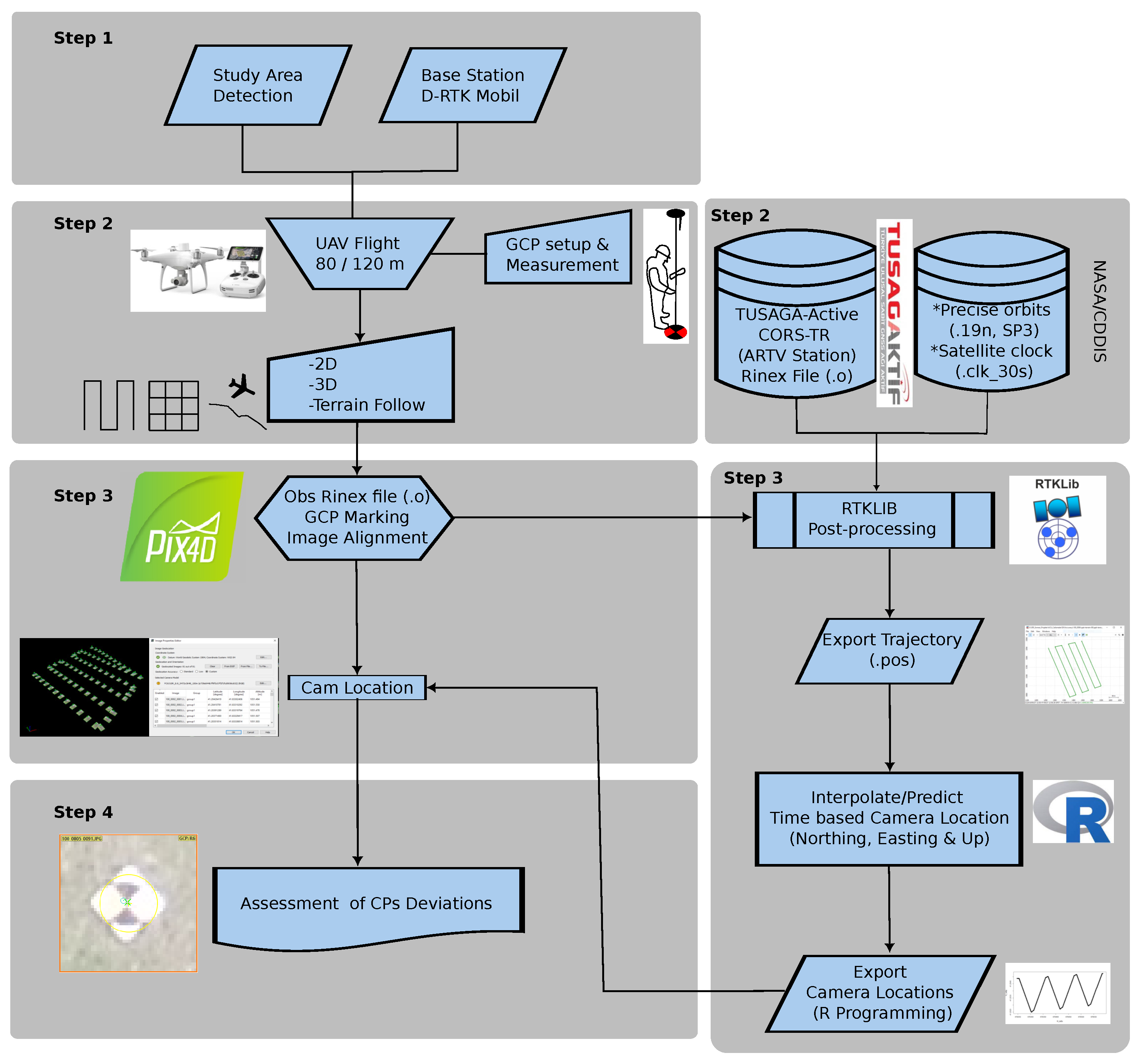
2.2. Methodology
- Mission planning (field survey, pre-flight and flight parameter settings);
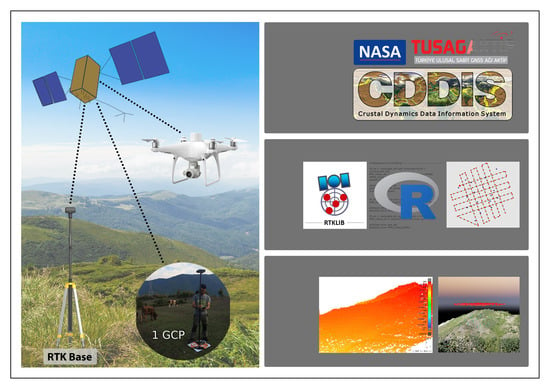
- Data collection (ground control and checkpoint placement and survey, UAV image acquisition, camera calibration, 1-s Continuously Operating Reference Station-Türkiye (CORS-TR) data);
- Data processing based on various techniques (bundle block adjustment and image-based matching, RTK and PPK data processing);
- Horizontal and vertical accuracy evaluation (data and error analysis, evaluation of camera and checkpoint (CP) coordinate differences).

2.3. Data Collection
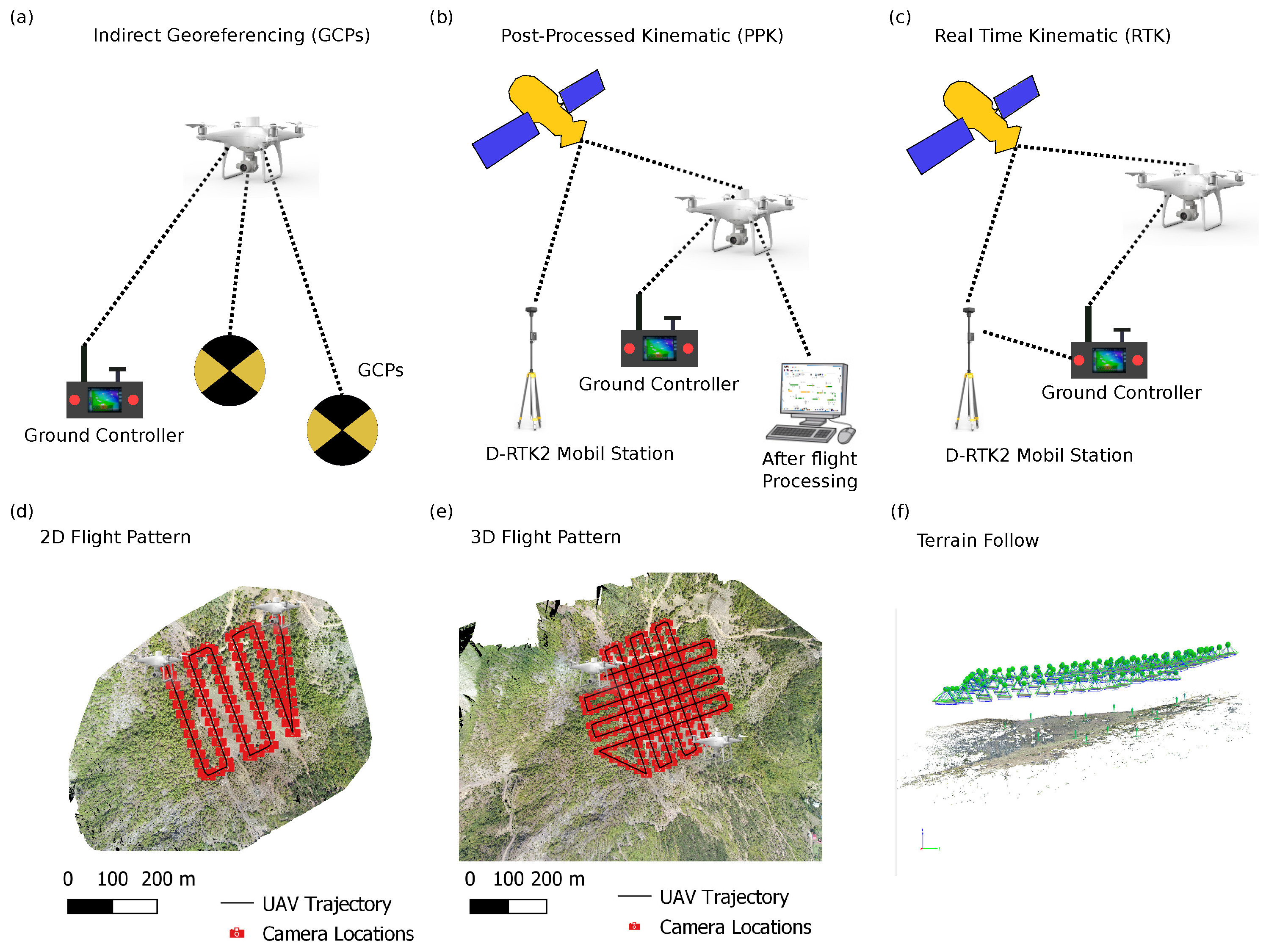
2.3.1. Ground Control Points
2.3.2. Real-Time Kinematic (RTK)
2.3.3. Post-Processing Kinematic (PPK)
2.4. Image Processing
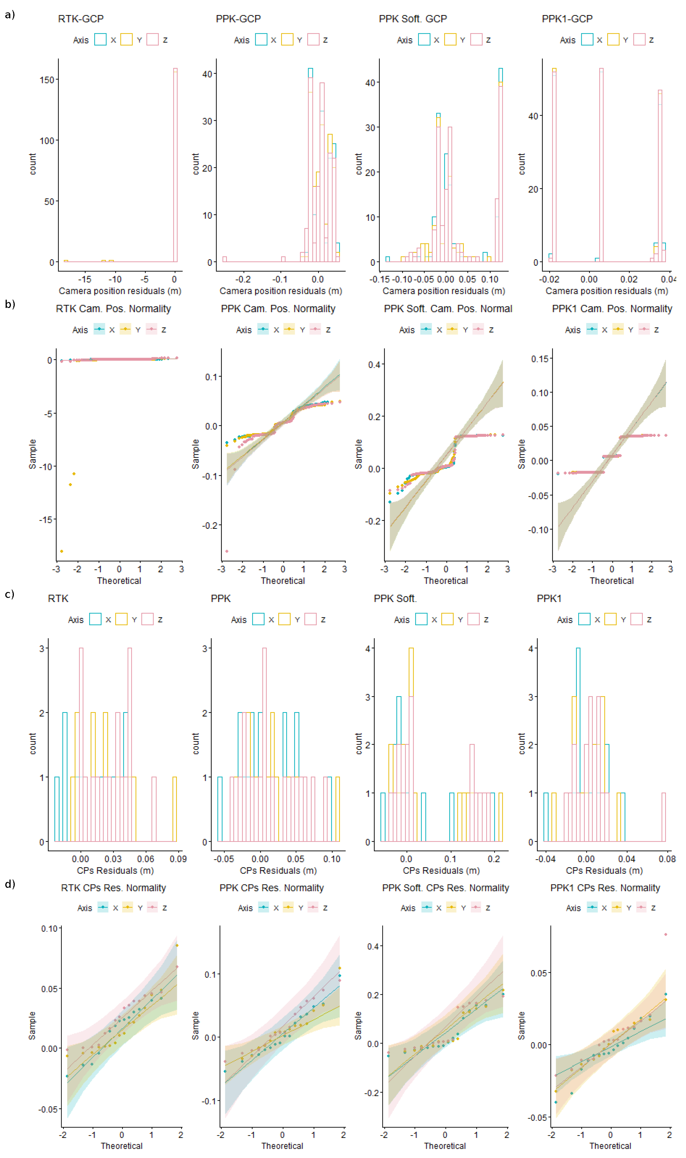
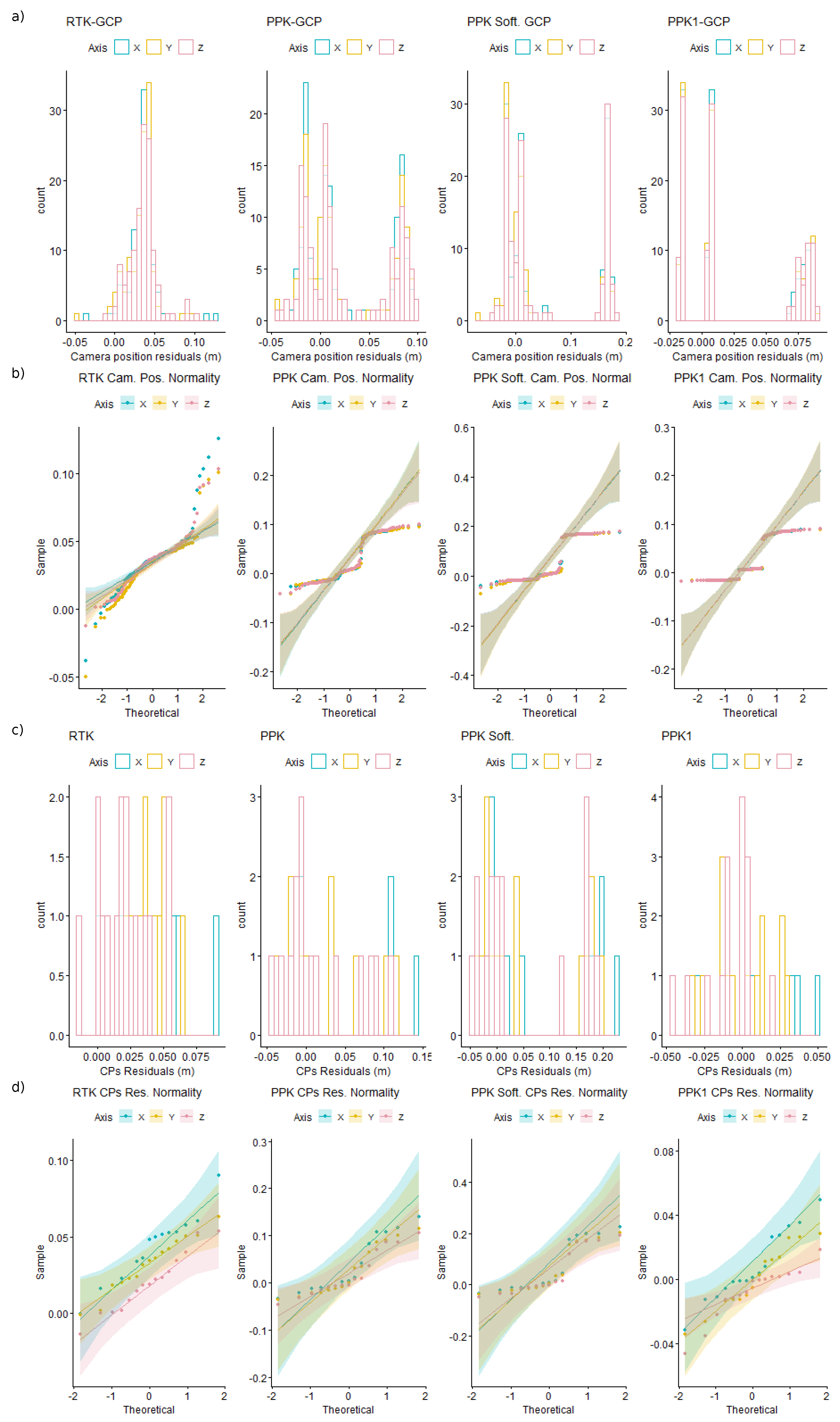
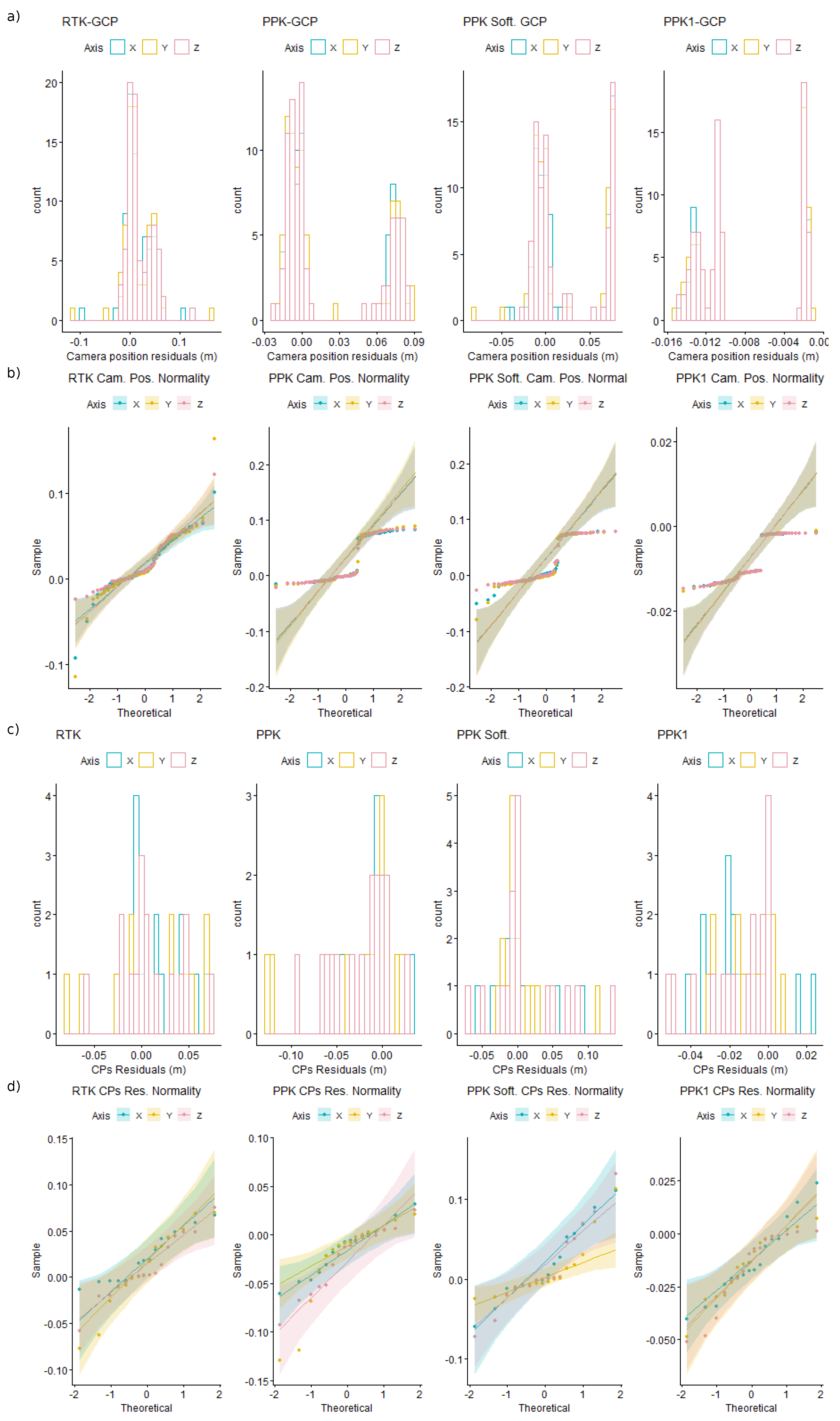
2.5. Accuracy Assessment
3. Results
3.1. Accuracy of RTK Ground Control Points
3.2. Accuracy of Post-Processing Kinematic
3.3. Accuracy of Post-Processing Kinematic and 1 GCP
4. Discussion
5. Conclusions
Author Contributions
Funding
Data Availability Statement
Acknowledgments
Conflicts of Interest
Abbreviations
| 2D | two-dimensional |
| 3D | three-dimensional |
| ARTV | Artvin |
| ASPRS | American Society for Photogrammetry and Remote Sensing |
| BBA | bundle block adjustment |
| CDDIS | Crustal Dynamics Data Information System |
| CP | checkpoint |
| CORS-TR | Continuously Operating Reference Station-Türkiye |
| ÇOMÜ | Çanakkale onsekiz mart üniversitesi |
| DRTK2 | DJI D-RTK 2 mobile station |
| DSM | digital surface model |
| EPSG | European petroleum survey group |
| GCP | ground control point |
| GCS | ground control station |
| GMT | Greenwich mean time |
| GNSS | Global Navigational Satellite Systems |
| GSD | ground sampling distance |
| IGS | International GNSS Service |
| IMU | Inertial Measurement Unit |
| INS | Inertial Navigation Systems |
| KML | keyhole markup language |
| Lat | latitude |
| Long | longitude |
| M3C2 | multiscale model to model cloud comparison |
| MVS | multi-view stereo |
| NASA | National Aeronautics and Space Administration |
| PPK | post-processing kinematic |
| PPM | part-per-million |
| RINEX | Receiver Independent Exchange Format |
| RMSE | root mean square error |
| RPAS | remotely piloted aircraft systems |
| RTK | real-time kinematic |
| SfM | structure from motion |
| TM | transverse mercator |
| TUREF | Turkish national reference frame |
| UAS | unmanned aerial system |
| UAV | unmanned aerial vehicle |
Appendix A


References
- Czapiewski, S. Assessment of the Applicability of UAV for the Creation of Digital Surface Model of a Small Peatland. Front. Earth Sci. 2022, 10, 834923. [Google Scholar] [CrossRef]
- Brovkina, O.; Cienciala, E.; Surový, P.; Janata, P. Unmanned aerial vehicles (UAV) for assessment of qualitative classification of Norway spruce in temperate forest stands. Geo-Spat. Inf. Sci. 2018, 21, 12–20. [Google Scholar] [CrossRef]
- Garg, P. Unmanned Aerial Vehicles; Mercury Learning and Information: Herndon, VA, USA, 2021. [Google Scholar]
- Kovanič, L.; Blistan, P.; Rozložník, M.; Szabó, G. UAS RTK/PPK photogrammetry as a tool for mapping the urbanized landscape, creating thematic maps, situation plans and DEM. Acta Montan. Slovaca 2022, 26, 649–660. [Google Scholar] [CrossRef]
- Padró, J.C.; Muñoz, F.J.; Planas, J.; Pons, X. Comparison of four UAV georeferencing methods for environmental monitoring purposes focusing on the combined use with airborne and satellite remote sensing platforms. Int. J. Appl. Earth Obs. Geoinf. 2019, 75, 130–140. [Google Scholar] [CrossRef]
- Taddia, Y.; Stecchi, F.; Pellegrinelli, A. Coastal mapping using dji phantom 4 RTK in post-processing kinematic mode. Drones 2020, 4, 9. [Google Scholar] [CrossRef]
- Erenoglu, R.C.; Erenoglu, O.; Arslan, N. Accuracy Assessment of Low Cost UAV Based City Modelling for Urban Planning. Teh. Vjesn.—Tech. Gaz. 2018, 25, 1708–1714. [Google Scholar] [CrossRef]
- Zeybek, M.; Biçici, S. Road Distress Measurements Using UAV. Türk Uzaktan Algılama CBS Dergisi 2020, 1, 13–23. [Google Scholar]
- Mancini, F.; Dubbini, M.; Gattelli, M.; Stecchi, F.; Fabbri, S.; Gabbianelli, G. Using unmanned aerial vehicles (UAV) for high-resolution reconstruction of topography: The structure from motion approach on coastal environments. Remote Sens. 2013, 5, 6880–6898. [Google Scholar] [CrossRef]
- Carrera-Hernández, J.J.; Levresse, G.; Lacan, P. Is UAV-SfM surveying ready to replace traditional surveying techniques? Int. J. Remote Sens. 2020, 41, 4818–4835. [Google Scholar] [CrossRef]
- Barry, P.; Coakley, R. Fiedl Accuracy Test of RPAS Photogrammetry. Int. Arch. Photogramm. Remote Sens. Spat. Inf. Sci. 2013, XL-1/W2, 27–31. [Google Scholar] [CrossRef]
- Furukawa, Y.; Ponce, J. Accurate, Dense, and Robust Multiview Stereopsis. IEEE Trans. Pattern Anal. Mach. Intell. 2010, 32, 1362–1376. [Google Scholar] [CrossRef] [PubMed]
- Elkhrachy, I. 3D Structure from 2D Dimensional Images Using Structure from Motion Algorithms. Sustainability 2022, 14, 5399. [Google Scholar] [CrossRef]
- Bemis, S.P.; Micklethwaite, S.; Turner, D.; James, M.R.; Akciz, S.; Thiele, S.T.; Bangash, H.A. Ground-based and UAV-Based photogrammetry: A multi-scale, high-resolution mapping tool for structural geology and paleoseismology. J. Struct. Geol. 2014, 69, 163–178. [Google Scholar] [CrossRef]
- Westoby, M.; Brasington, J.; Glasser, N.; Hambrey, M.; Reynolds, J. ‘Structure-from-Motion’ photogrammetry: A low-cost, effective tool for geoscience applications. Geomorphology 2012, 179, 300–314. [Google Scholar] [CrossRef]
- Eltner, A.; Hoffmeister, D.; Kaiser, A.; Karrasch, P.; Klingbeil, L.; Stöcker, C.; Rovere, A. UAVs for the Environmental Sciences Methods and Applications; wbg Academic: Darmstadt, Germany, 2022. [Google Scholar]
- Nesbit, P.R.; Hubbard, S.M.; Hugenholtz, C.H. Direct Georeferencing UAV-SfM in High-Relief Topography: Accuracy Assessment and Alternative Ground Control Strategies along Steep Inaccessible Rock Slopes. Remote Sens. 2022, 14, 490. [Google Scholar] [CrossRef]
- Zeybek, M.; Biçici, S. 3D Dense Reconstruction of Road Surface from UAV Images and Comparison of SfM Based Software Performance. Turk. J. Remote Sens. GIS 2021, 2, 96–105. [Google Scholar] [CrossRef]
- Famiglietti, N.A.; Cecere, G.; Grasso, C.; Memmolo, A.; Vicari, A. A Test on the Potential of a Low Cost Unmanned Aerial Vehicle RTK/PPK Solution for Precision Positioning. Sensors 2021, 21, 3882. [Google Scholar] [CrossRef] [PubMed]
- Zhang, H.; Aldana-Jague, E.; Clapuyt, F.; Wilken, F.; Vanacker, V.; Van Oost, K. Evaluating the potential of post-processing kinematic (PPK) georeferencing for UAV-based structure- from-motion (SfM) photogrammetry and surface change detection. Earth Surf. Dyn. 2019, 7, 807–827. [Google Scholar] [CrossRef]
- Belloni, V.; Fugazza, D.; Di Rita, M. UAV-Based Glacier Monitoring: GNSS Kinematic Track Post-processing and Direct Georeferencing for Accurate Reconstructions in Challenging Environments. Int. Arch. Photogramm. Remote Sens. Spat. Inf. Sci. 2022, XLIII-B1-2, 367–373. [Google Scholar] [CrossRef]
- Bláha, M.; Eisenbeiss, H.; Grimm, D.; Limpach, P. Direct georeferencing of UAVS. Int. Arch. Photogramm. Remote Sens. Spat. Inf. Sci. 2012, XXXVIII-1, 131–136. [Google Scholar] [CrossRef]
- Whitehead, K.; Hugenholtz, C.H. Applying ASPRS Accuracy Standards to Surveys from Small Unmanned Aircraft Systems (UAS). Photogramm. Eng. Remote Sens. 2015, 81, 787–793. [Google Scholar] [CrossRef]
- Agüera-Vega, F.; Carvajal-Ramírez, F.; Martínez-Carricondo, P. Assessment of photogrammetric mapping accuracy based on variation ground control points number using unmanned aerial vehicle. Measurement 2017, 98, 221–227. [Google Scholar] [CrossRef]
- James, M.R.; Robson, S.; D’Oleire-Oltmanns, S.; Niethammer, U. Optimising UAV topographic surveys processed with structure-from-motion: Ground control quality, quantity and bundle adjustment. Geomorphology 2017, 280, 51–66. [Google Scholar] [CrossRef]
- Elkhrachy, I. Accuracy Assessment of Low-Cost Unmanned Aerial Vehicle (UAV) Photogrammetry. Alex. Eng. J. 2021, 60, 5579–5590. [Google Scholar] [CrossRef]
- Iizuka, K.; Ogura, T.; Akiyama, Y.; Yamauchi, H.; Hashimoto, T.; Yamada, Y. Improving the 3D model accuracy with a post-processing kinematic (PPK) method for UAS surveys. Geocarto Int. 2022, 37, 4234–4254. [Google Scholar] [CrossRef]
- Liu, X.; Lian, X.; Yang, W.; Wang, F.; Han, Y.; Zhang, Y. Accuracy Assessment of a UAV Direct Georeferencing Method and Impact of the Configuration of Ground Control Points. Drones 2022, 6, 30. [Google Scholar] [CrossRef]
- Salas López, R.; Terrones Murga, R.E.; Silva-López, J.O.; Rojas-Briceño, N.B.; Gómez Fernández, D.; Oliva-Cruz, M.; Taddia, Y. Accuracy Assessment of Direct Georeferencing for Photogrammetric Applications Based on UAS-GNSS for High Andean Urban Environments. Drones 2022, 6, 388. [Google Scholar] [CrossRef]
- Cirillo, D.; Cerritelli, F.; Agostini, S.; Bello, S.; Lavecchia, G.; Brozzetti, F. Integrating Post-Processing Kinematic (PPK)–Structure-from-Motion (SfM) with Unmanned Aerial Vehicle (UAV) Photogrammetry and Digital Field Mapping for Structural Geological Analysis. ISPRS Int. J. Geo-Inf. 2022, 11, 437. [Google Scholar] [CrossRef]
- Zeybek, M. Accuracy assessment of direct georeferencing UAV images with onboard global navigation satellite system and comparison of CORS/RTK surveying methods. Meas. Sci. Technol. 2021, 32, 065402. [Google Scholar] [CrossRef]
- Yildirim, Ö.; Mekik, Ç.; Bakici, S. TUSAGA-AKTİF CORS-TR Sisteminin Tapu ve Kadastro Genel Müdürlüğüne Katkıları. Jeodezi Jeoinformasyon Derg. 2011, 104, 134–139. [Google Scholar]
- Estey, L.H.; Meertens, C.M. TEQC: The Multi-Purpose Toolkit for GPS/GLONASS Data. GPS Solut. 1999, 3, 42–49. [Google Scholar] [CrossRef]
- Noll, C.E. The crustal dynamics data information system: A resource to support scientific analysis using space geodesy. Adv. Space Res. 2010, 45, 1421–1440. [Google Scholar] [CrossRef]
- Takasu, T.; Yasuda, A. Development of the low-cost RTK-GPS receiver with an open source program package RTKLIB. In Proceedings of the International Symposium on GPS/GNSS, Seogwipo-si, Republic of Korea, 4–6 November 2009; Volume 1, pp. 1–6. [Google Scholar]
- Cleveland, W.S.; Grosse, E.; Shyu, W.M. Local Regression Models. In Statistical Models in S; Routledge: Oxfordshire, UK, 2017; Volume 35, pp. 309–376. [Google Scholar] [CrossRef]
- R Core Team. R: A Language and Environment for Statistical Computing; R Foundation for Statistical Computing: Vienna, Austria, 2022. [Google Scholar]
- Cleveland, W.S.; Devlin, S.J. Locally weighted regression: An approach to regression analysis by local fitting. J. Am. Stat. Assoc. 1988, 83, 596–610. [Google Scholar] [CrossRef]
- Kuhn, M.; Johnson, K. Applied Predictive Modeling; Springer Nature: Berlin/Heidelberg, Germany, 2013; pp. 1–600. [Google Scholar] [CrossRef]
- Arnold, T.; Kane, M.; Lewis, B.W. Linear Smoothers; CRC Press: Boca Raton, FL, USA, 2019; pp. 75–122. [Google Scholar] [CrossRef]
- Ruppert, D.; Matteson, D.S. Statistics and Data Analysis for Financial Engineering; Springer Texts in Statistics; Springer: New York, NY, USA, 2015; pp. 75–122. [Google Scholar] [CrossRef]


| Flight Height | ||
|---|---|---|
| Capture Mode | 80 m | 120 m |
| RTK/PPK 2D | 3.42 | 4.66 |
| RTK/PPK 3D | NA | 6.50 |
| (RTK/PPK) Terrain-Following | 1.87 | 3.12 |
| Method | Altitude | (m) | (m) |
|---|---|---|---|
| RTK 2D | 80 m | 0.038 | 0.039 |
| 120 m | 0.044 | 0.046 | |
| PPK 2D | 80 m | 0.033 | 0.059 |
| 120 m | 0.031 | 0.062 | |
| PPK1 2D | 80 m | 0.023 * | 0.024 * |
| 120 m | 0.019 | 0.033 | |
| PPK Soft. 2D | 80 m | 0.033 | 0.157 |
| 120 m | 0.032 | 0.073 | |
| RTK 3D | 80 m | - | - |
| 120 m | 0.044 | 0.115 | |
| PPK 3D | 80 m | - | - |
| 120 m | 0.020 | 0.130 | |
| PPK1 3D | 80 m | - | - |
| 120 m | 0.014 ** | 0.088 | |
| PPK Soft. 3D | 80 m | - | - |
| 120 m | 0.026 | 0.046 | |
| RTK Terrain-Following | 80 m | 0.045 | 0.047 |
| 120 m | 0.040 | 0.050 | |
| PPK Terrain-Following | 80 m | 0.030 | 0.096 |
| 120 m | 0.045 | 0.094 | |
| PPK1 Terrain-Following | 80 m | 0.024 | 0.025 |
| 120 m | 0.035 | 0.032 ** | |
| PPK Soft. Terrain-Following | 80 m | 0.033 | 0.181 |
| 120 m | 0.040 | 0.050 |
Disclaimer/Publisher’s Note: The statements, opinions and data contained in all publications are solely those of the individual author(s) and contributor(s) and not of MDPI and/or the editor(s). MDPI and/or the editor(s) disclaim responsibility for any injury to people or property resulting from any ideas, methods, instructions or products referred to in the content. |
© 2023 by the authors. Licensee MDPI, Basel, Switzerland. This article is an open access article distributed under the terms and conditions of the Creative Commons Attribution (CC BY) license (https://creativecommons.org/licenses/by/4.0/).
Share and Cite
Zeybek, M.; Taşkaya, S.; Elkhrachy, I.; Tarolli, P. Improving the Spatial Accuracy of UAV Platforms Using Direct Georeferencing Methods: An Application for Steep Slopes. Remote Sens. 2023, 15, 2700. https://doi.org/10.3390/rs15102700
Zeybek M, Taşkaya S, Elkhrachy I, Tarolli P. Improving the Spatial Accuracy of UAV Platforms Using Direct Georeferencing Methods: An Application for Steep Slopes. Remote Sensing. 2023; 15(10):2700. https://doi.org/10.3390/rs15102700
Chicago/Turabian StyleZeybek, Mustafa, Selim Taşkaya, Ismail Elkhrachy, and Paolo Tarolli. 2023. "Improving the Spatial Accuracy of UAV Platforms Using Direct Georeferencing Methods: An Application for Steep Slopes" Remote Sensing 15, no. 10: 2700. https://doi.org/10.3390/rs15102700