Article

Tree Species Classification in Subtropical Natural Forests Using High-Resolution UAV RGB and SuperView-1 Multispectral Imageries Based on Deep Learning Network Approaches: A Case Study within the Baima Snow Mountain National Nature Reserve, China

Co-Innovation Center for Sustainable Forestry in Southern China, Nanjing Forestry University, Nanjing 210037, China
*
Author to whom correspondence should be addressed.
Remote Sens. 2023, 15(10), 2697; https://doi.org/10.3390/rs15102697
Submission received: 22 March 2023 / Revised: 8 May 2023 / Accepted: 19 May 2023 / Published: 22 May 2023
(This article belongs to the Section Forest Remote Sensing)

Abstract

:
Accurate information on dominant tree species and their spatial distribution in subtropical natural forests are key ecological monitoring factors for accurately characterizing forest biodiversity, depicting the tree competition mechanism and quantitatively evaluating forest ecosystem stability. In this study, the subtropical natural forest in northwest Yunnan province of China was selected as the study area. Firstly, an object-oriented multi-resolution segmentation (MRS) algorithm was used to segment individual tree crowns from the UAV RGB imagery and satellite multispectral imagery in the forests with different densities (low (547 n/ha), middle (753 n/ha) and high (1040 n/ha)), and parameters of the MRS algorithm were tested and optimized for accurately extracting the tree crown and position information of the individual tree. Secondly, the texture metrics of the UAV RGB imagery and the spectral metrics of the satellite multispectral imagery within the individual tree crown were extracted, and the random forest algorithm and three deep learning networks constructed in this study were utilized to classify the five dominant tree species. Finally, we compared and evaluated the performance of the random forest algorithm and three deep learning networks for dominant tree species classification using the field measurement data, and the influence of the number of training samples on the accuracy of dominant tree species classification using deep learning networks was investigated. The results showed that: (1) Stand density had little influence on individual tree segmentation using the object-oriented MRS algorithm. In the forests with different stand densities, the F1 score of individual tree segmentation based on satellite multispectral imagery was 71.3–74.7%, and that based on UAV high-resolution RGB imagery was 75.4–79.2%. (2) The overall accuracy of dominant tree species classification using the light-weight network MobileNetV2 (OA = 71.11–82.22%), residual network ResNet34 (OA = 78.89–91.11%) and dense network DenseNet121 (OA = 81.11–94.44%) was higher than that of the random forest algorithm (OA = 60.00–64.44%), among which DenseNet121 had the highest overall accuracy. Texture metrics improved the overall accuracy of dominant tree species classification. (3) For the three deep learning networks, the changes in overall accuracy of dominant tree species classification influenced by the number of training samples were 2.69–4.28%.

1. Introduction

As the main part of the terrestrial ecosystem, forests play an important role in maintaining biodiversity, improving the ecological environment and mitigating climate change [1,2,3]. Natural forests have abundant biodiversity, which is essential for maintaining the stability of forest ecosystems [4,5,6]. Trees are the foundation of the forest ecosystem, and the composition of tree species is one of the key indicators to measure forest biodiversity [7]. The composition and spatial distribution of tree species are critical for forest resource management and forest biodiversity monitoring [8], which can be also used as an indicator of species richness to assess the potential of forest ecosystem services [9], explore aboveground biomass changes [10] and reveal competition among tree species [11]. The traditional method of obtaining tree species information mainly depends on the field inventory. However, this is time-consuming and labor-intensive [12,13]. Furthermore, tree species information is typically collected using sample plots, so the spatially continuous information is normally ignored [7]. Particularly in the natural forests with complex structures, it is difficult to obtain the fine-scale spatial distribution of tree species using a field inventory approach [14]. Remote sensing can provide multi-dimensional and spatially continuous information on forests, which makes it possible to access tree species composition in a timely and efficient manner [15].
Multispectral remote sensing can provide lots of spectral (or texture) and spatially continuous information about forests, which plays a key role in the identification of tree species [16,17]. However, due to the limitations of spatial and spectral resolution, traditional optical imagery is normally used to classify forest types [18]. Yu et al. [19] used SPOT-5 imagery to identify forest types in Pangu Forest Farm in the Daxing’an Mountains, and the overall accuracy of classification was 76.0%. With an improvement in spatial and spectral resolution, optical imagery can be used to identify the dominant tree species [20]. Cho et al. [21] used high-resolution WorldView-2 imagery (resolution = 0.5–2 m) to classify three dominant tree species in the native forests of South Africa, with an overall accuracy of 87.2–91.4%. Immitzer et al. [14] used 8-band WorldView-2 imagery combined with the random forest algorithm to classify 10 types of tree species in temperate forests, and the overall accuracy was 82.0%. Moreover, the combination of spectral indices and texture metrics can generally improve the accuracy of dominant tree species classification [22,23]. Deur et al. [24] used multispectral WorldView-3 satellite imagery to classify dominant tree species in deciduous mixed forests. The results showed that the overall accuracy of classification can be improved by 7.0–10.0% after adding texture metrics. Ferreira et al. [25] classified eight dominant tree species from Brazil’s semi-deciduous forests using the visible bands of WorldView-3 imagery combined with texture metrics. Compared with using the visible bands only, the average producer accuracy was improved by 22.0–34.0%.
Unmanned aerial vehicles (UAVs) can operate at a lower attitude to obtain ultra-high spatial resolution data [26]. In recent years, due to the advantages of low cost, high efficiency and fine precision, the application of UAVs in assessing forest regeneration, monitoring forest health and detecting individual trees has increased rapidly. Reis et al. [27] used UAVs to access multispectral images and classify them to evaluate the status of forest renewal, and the performance was good (OA = 94.0%). Dash et al. [28] obtained multispectral images of time series based on UAVs and simulated early stress on trees using non-parametric methods, which had a high classification accuracy (kappa = 0.694). Nuijten et al. [29] used a digital aerial photogrammetry point cloud (DAP) acquired via UAVs to segment individual tree crowns of deciduous forests in different seasons, with an accuracy of 55.0–77.1%. The high-resolution imagery of UAVs contains fine-scale forest canopy information [30], which can be used for the segmentation and detection of individual tree crowns. Marques et al. [31] used the clustering segmentation method to segment Chestnut trees from UAV high-resolution imagery with an accuracy of 97.0%. The object-oriented multi-resolution segmentation (MRS) algorithm aims to divide remote sensing imagery into objects with the same shape or spectral characteristics [32], in which the spectral variation in various ground objects could be reduced so the statistical and classification accuracy could be properly improved [33,34]. Xu et al. [35] used the MRS algorithm to segment individual trees from high-resolution RGB ortho-imagery, and the accuracy was 76.9%. However, most of the previous studies applied the MRS algorithm to plantation or the forest stands with simple structures, and there are few studies on the extraction of individual trees using the MRS algorithm in subtropical natural forests.
Deep learning is an algorithm that uses successive neural layers to reveal deeper features and more metaphysical information of images [36]. A convolutional neural network (CNN) in deep learning is commonly used to analyze the spatial features of remote sensing images, such as edges and textures, which could be suitable for tree species identification [37]. Natesan et al. [38] used a residual convolutional network to classify three types of tree species, named red pine, white pine and non-pine, in a coniferous mixed forest, with an overall classification of 80.1%. Schiefer et al. [37] used a U-Net convolutional neural network to classify nine dominant tree species in temperate forests, and the overall classification was 83.2%. Meanwhile, previous studies showed that the combination of CNN and high-resolution satellite images had a high accuracy for the identification of dominant tree species in mixed forests. Guo et al. [39] used three types of convolutional neural networks combined with WorldView-3 imagery to classify seven types of tree species in coniferous and broadleaf mixed forests. The results showed that the DenseNet model had the highest classification accuracy (OA = 75.1–78.1%). Yan et al. [40] used five types of CNN models combined with WorldView-3 imagery to classify six dominant tree species in a mixed plantation, and the results showed that the improved GoogLeNet model had the highest classification accuracy (OA = 82.7%). Compared with traditional machine learning algorithms, deep learning networks can improve the accuracy of dominant tree species classification [41]. Onishi et al. [42] used a ResNet model to classify dominant tree species in coniferous mixed forests. Compared with the support vector machine algorithm, the overall classification accuracy was improved by 5.8–13.1%. Zhang et al. [43] used ResNet50, KNN and BP neural network algorithms to classify 10 types of urban tree species, and the results showed that the overall accuracy of ResNet50 was, on average, 30% higher than KNN and BP neural network algorithms. However, there are few studies combining deep learning network algorithms with multi-source remote sensing data for dominant tree species classification, and the potential of using deep learning network algorithms to identify the dominant tree species in subtropical natural forests needs to be explored.
In view of the above research gaps, this study selected a subtropical natural forest in northwest Yunnan province of China as the study area and obtained high-resolution ortho-imagery (spatial resolution = 0.23 m) based on a fixed-wing UAV and sub-meter (spatial resolution = 0.5 m) multispectral imagery based on the SuperView-1 satellite. The random forest algorithm and three deep learning networks (lightweight network MobileNetV2, residual network ResNet34 and dense network DenseNet121) were constructed to classify the five dominant tree species. The main objectives of this paper are as follows: (1) to compare the segmentation accuracy of individual trees in forests with different stand densities (low (547 n/ha), middle (753 n/ha) and high (1040 n/ha)) from UAV high-resolution ortho-imagery and satellite multispectral imagery; (2) to compare and evaluate the overall accuracy of three deep learning networks and random forest algorithms combined with spectral and texture metrics for dominant tree species classification in natural forests; (3) to explore the variations in the overall accuracy of dominant tree species classification using three deep learning networks while reducing the number of training samples.
The workflow containing several steps of data processing is shown in Figure 1. In this study, we obtained high-resolution images from fixed-wing UAVs and multispectral imagery from the SuperView-1 satellite and then combined these with an individual tree segmentation algorithm, machine learning and multiple deep learning networks to identify the dominant tree species in the subtropical natural forests of northwest Yunnan province. Firstly, the RGB images obtained by the UAV were aligned to generate high-resolution ortho-imagery. Secondly, the object-oriented MRS algorithm was used to generate individual tree crown boundaries. Finally, the extracted individual tree crown metrics (i.e., multispectral and texture metrics) were combined with the random forest algorithm and three deep learning networks to classify the five dominant tree species.

2. Materials and Methods
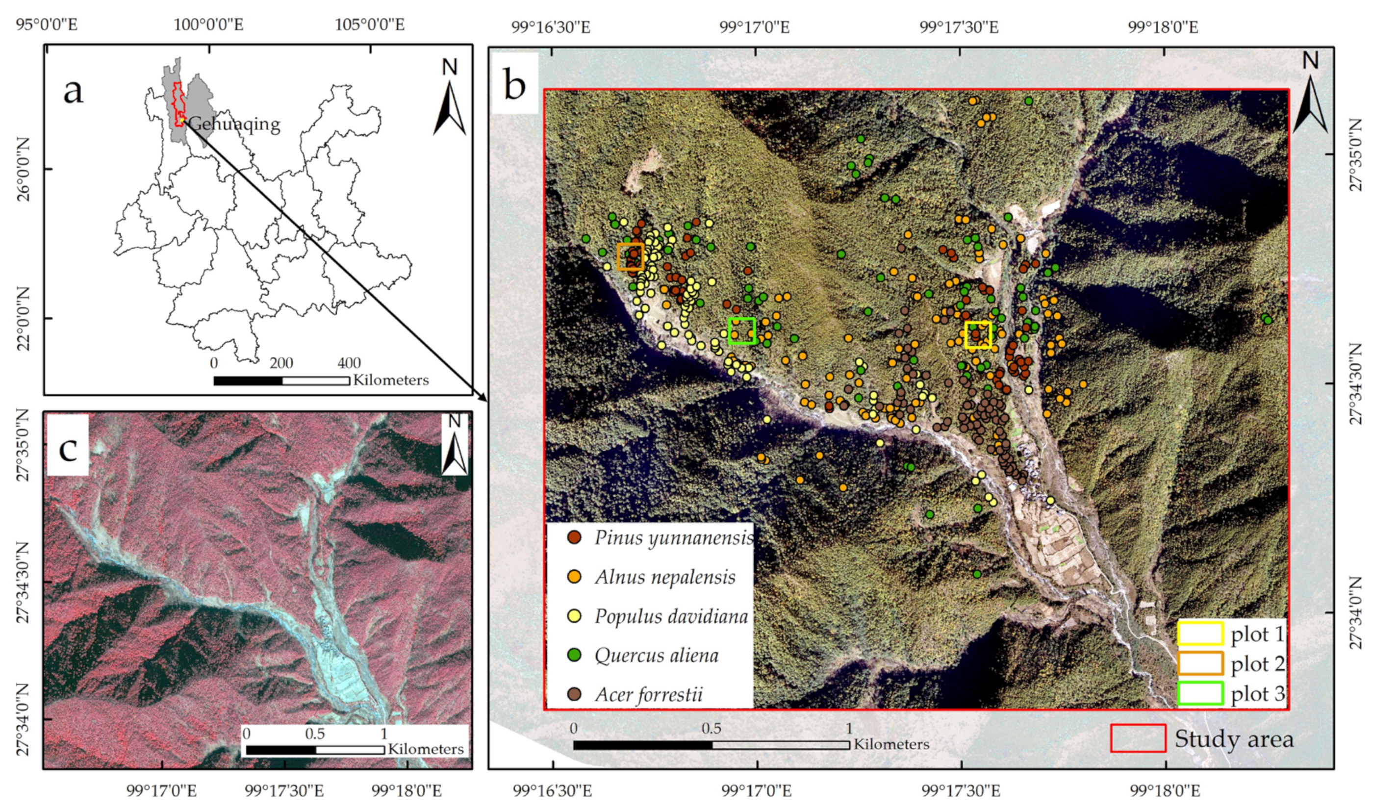
2.1. Study Area

Gehuaqing (GHQ) is located in Weixi County, south of Diqing Tibetan Autonomous Prefecture, Northwest Yunnan Province of China, and the south of Baima Snow Mountain National Nature Reserve (98°57′–99°25′E, 27°24′–28°36′N), as shown in Figure 2. The elevation ranges from 2100 m to 3500 m. The study area belongs to the plateau mountain monsoon climate, which can be divided into two seasons: dry and wet. In the winter half year (November to April of the next year), the weather is sunny, and rainfall is reduced, showing the characteristics of dry season climate, while in the summer half year (May to October), the study area has more clouds and concentrated rain, forming the rainy season. The annual average temperature is 9.5 °C, the average temperature of the coldest month (January) is 1.5 °C and that of hottest month (July) is 17.3 °C. The annual average rainfall is 845.1 mm. The rate of forest coverage in the study area is 76.2%, and the dominant forest types can be divided into cold temperate conifer forests and deciduous broadleaf forests. The dominant conifer species is Yunnan pine (Pinus yunnanensis), and the dominant broadleaf species can be divided into four types: Nepal alder (Alnus nepalensis), aspen (Populus davidiana), Oriental white oak (Quercus aliena) and maple (Acer forrestii).

2.2. Field Measurements

Considering factors, such as altitude, slope and tree species types, a total of 450 trees in the study area were selected and measured. The measurement includes individual tree species and position information, diameter at breast height, tree top height and crown width. The position of the individual tree was recorded using a Trimble® real-time kinematic (RTK) R4 GNSS with centimeter-level accuracy. The tree top height was measured via Vertex IV® hypsometer. The tape was used to measure crown width, and the results were expressed as the average of two values measured in vertical directions of tree crown. Statistics for five dominant tree species parameters are aggregated in Table 1.

2.3. Remote Sensing Data

A fixed-wing UAV equipped with RGB camera (Sony ILCE-6000) was used to obtain RGB images from 7 November to 8 November 2018. The weather condition was clear without clouds. The UAV flew at an altitude of 800 m relative to the ground, with a speed of 20 m/s, a forward overlap ratio of more than 80% and the average ground sample distance was 0.23 m. The satellite multispectral imagery was shot by SuperView-1 satellite on 4 December 2018, with approximately 0% cloud cover and covering the whole study area. The multispectral imagery included five bands of panchromatic (450–890 nm), blue (450–520 nm), green (520–590 nm), red (630–690 nm) and near-infrared (690–890 nm), in which the spatial resolution of panchromatic band was 0.5 m and that of spectral bands was 2 m.

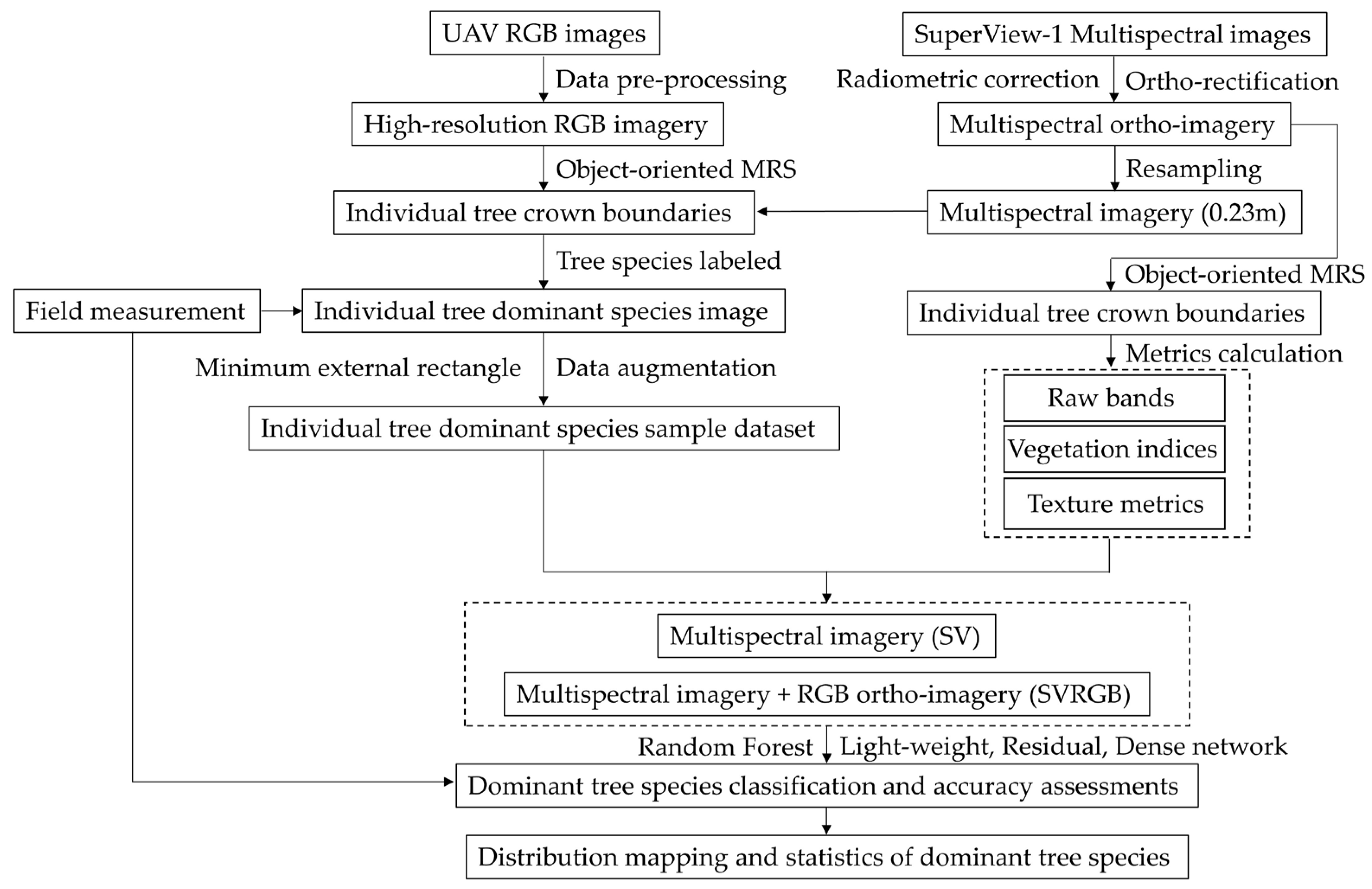
2.4. Data Pre-Processing

Before stitching RGB images, the RGB images with poor quality (including blurred images and images that did not reach the target height at the intersection point of the flight path) were removed. The images were matched using the GPS data and inertial measurement units (IMUs) during flight, and the matched images were stitched to obtain high-resolution RGB imagery.
The pre-processing of multispectral imagery included radiometric calibration, atmospheric correction and Rational Polynomial Coefficient (RPC) ortho-rectification. Firstly, radiometric calibration and atmospheric correction were used to convert digital number (DN) values into reflectance. Secondly, the image after ortho-rectification was fused by using the misalignment impact (RMI) fusion method [44] to obtain sub-meter-resolution multispectral imagery. Thirdly, 200 ground control points were selected from RGB and multispectral ortho-imageries to co-register the multispectral imagery to RGB imagery using spline algorithm, and the correction error was controlled within 0.01 m. Finally, the nearest neighbor method was used for resampling to obtain spatially matched RGB and multispectral ortho-imageries.

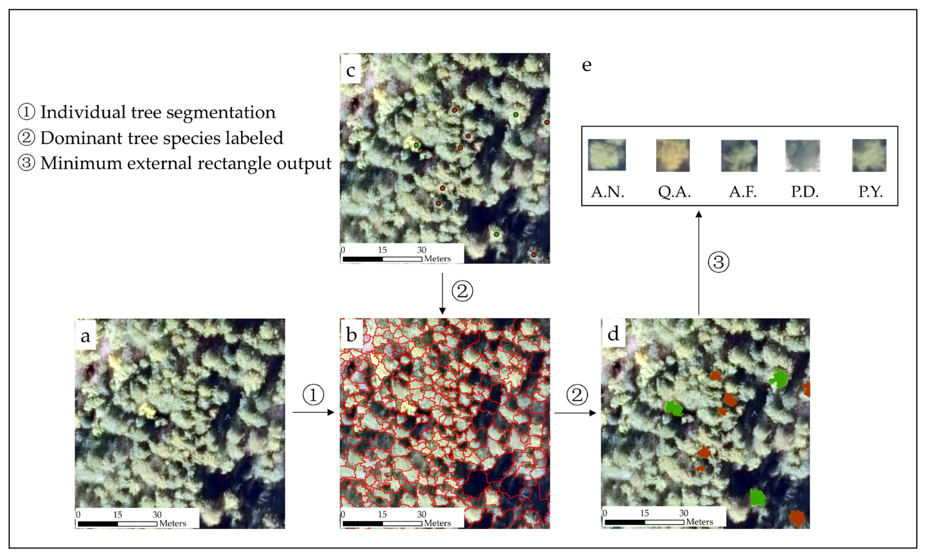
2.5. Sample Dataset of Individual Tree

The establishment of the sample dataset of individual trees was based on the pre-processed images, combined with the segmentation results and the position information of individual trees obtained from field measurement to generate the dominant tree species images, and minimum external rectangle method was used to output these images. The detailed process is shown in Figure 3. Firstly, the pre-processed image (Figure 3a) was segmented by an object-oriented MRS algorithm (Figure 3①) to generate the segmented image (Figure 3b). Secondly, combined with the position information of individual trees obtained from field measurement (Figure 3c), the dominant tree species types were labeled (Figure 3②) on the segmented image. Thirdly, the tree crown of each labeled dominant tree species type (Figure 3d) was output via minimum external rectangle (Figure 3③) method to obtain the tree crown images of individual tree dominant species (Figure 3e). Finally, data augmentation was performed based on tree crown images of dominant individual tree species to obtain a sample dataset for training.
With the help of the position of individual tree samples, the images were labeled and classified for the training of deep learning networks. The sample dataset of individual trees was divided into five types, including 118 Nepal alder (A.N.), 80 Oriental white oak (Q.A.), 97 Aspen (P.D.), 80 Maple (A.F.) and 75 Yunnan pine (P.Y.).

2.5.1. Data Augmentation

In this study, data augmentation was performed on the individual tree samples to increase the number of training samples. The data augmentation methods include rotation and brightening, such as rotating the image clockwise by 90°, counterclockwise by 90°, 180° and brightening by 50% [45,46,47,48]. After data augmentation, the number of sample datasets was increased to five times. A detailed description is shown in Table 2.
Training an epoch in a deep learning network represents complete model training with all the data of the training samples. To avoid network overfitting, the validation data were used to evaluate the accuracy of the deep learning network after each set of training. In this paper, 80% of the sample dataset was randomly selected for model training and 20% for model validation.

2.5.2. Remote Sensing Sample Dataset of Individual Trees

To take advantage of the texture metrics of high-resolution RGB imagery, the SuperView-1 satellite multispectral imagery (SV) was resampled and stacked with the RGB imagery (RGB) to obtain the post-stacked image (SVRGB). Therefore, multispectral and post-stacked images were used for dominant tree species classification and generated two individual tree sample datasets, named “SV” and “SVRGB”. All the sample datasets included 2250 samples and five dominant tree species (i.e., Nepal alder, Oriental white oak, Aspen, Maple and Yunnan pine). A detailed description is shown in Table 2.

2.6. Spectral and Texture Metrics Calculation

After the individual tree crowns were segmented, spectral data were extracted from the multispectral imagery, and a set of vegetation indices was calculated. Then, the high-resolution RGB imagery was used to calculate seven texture metrics of each band (blue, green and red band) for a total of 21 metrics. The meanings and calculation formulas for spectral indices variables and texture metrics of individual trees are shown in Table 3 and Table 4.

2.7. Random Forest and Deep Learning Network Classifier

2.7.1. Random Forest

Random forest algorithm creates several CART-like trees, and each tree is trained with the original training samples to vote on the most popular class of the input variables, and the output class is determined by the majority vote of the tree [58,59]. The training samples were used to train the random forest classifier, and the validation samples were used to evaluate the classification accuracy. The training and validation samples were randomly divided into 80% and 20% of the total samples for each tree species, respectively.

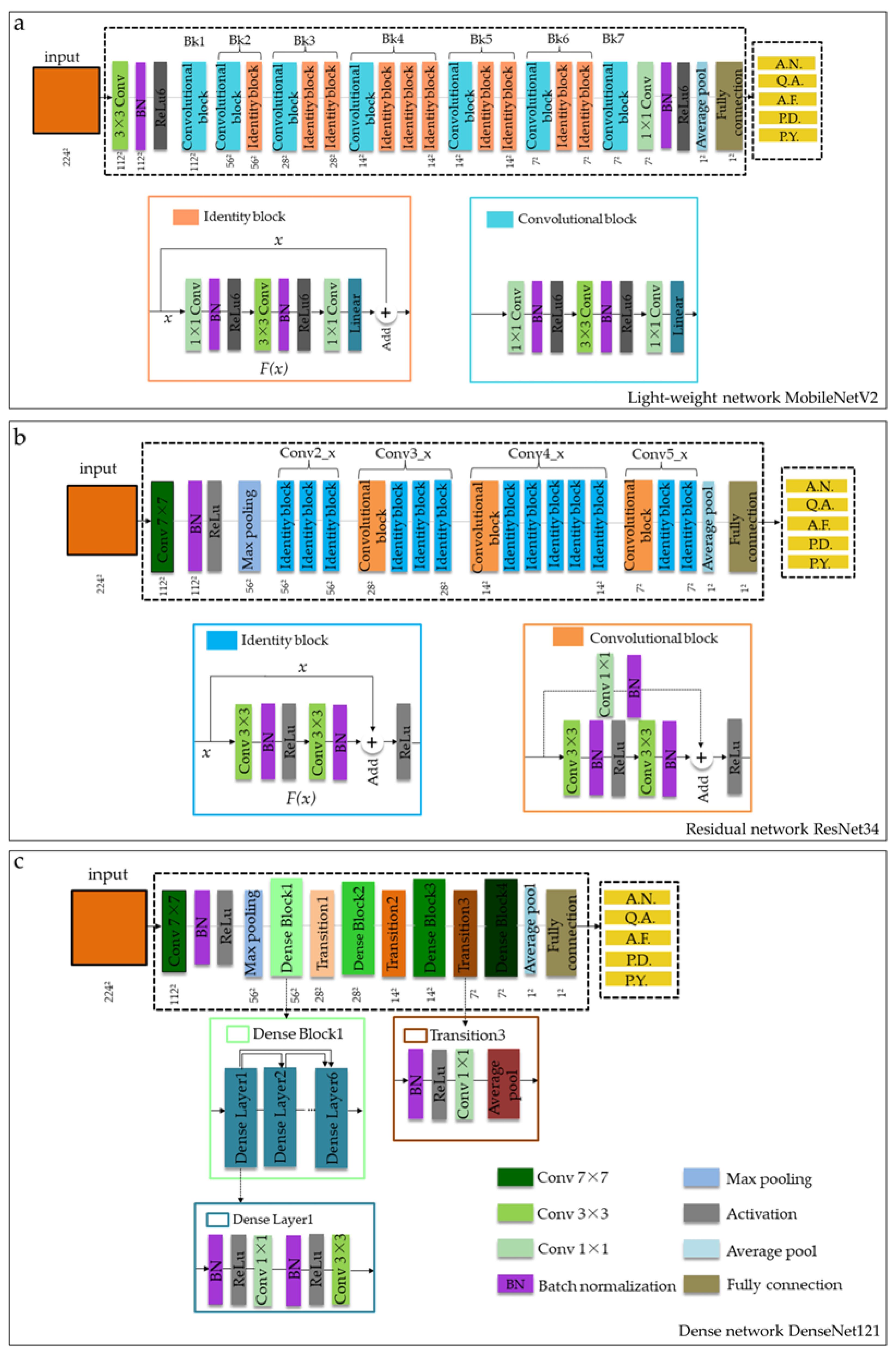
2.7.2. Deep Learning Networks

A deep learning network is a framework consisting of a stack of several convolutional layers, pooling layers and fully connected layers [38]. The convolutional layer is used to extract features from the input image, the pooling layer is responsible for reducing the dimension of the image and the fully connected layer classifies the image by probability. Three deep learning networks were used to classify dominant tree species in this study, namely, the lightweight network MobileNetV2 [60], the residual network ResNet34 [61] and the dense network DenseNet121 [62].
(1)
Lightweight network MobileNetV2
The core of the MobileNetV2 model is the “inverted residual structure”. In the structure, the tensor depth containing the input feature image is firstly boosted by 1 × 1 convolution; then, the output is provided to 3 × 3 depth-wise convolution, and finally, 1 × 1 convolution is used to reduce the dimension of the feature image. Each convolution is followed by batch normalization and ReLu6 activation functions. However, ReLu6 function can easily cause the loss of low-dimension feature information in the image; thus, linear activation function is selected in the dimensionality reduction stage.
The overview MobileNetV2 model is shown in Figure 4a. This framework consists of 55 training layers, including 2 regular convolutional layers, 17 inverted residual feature layers (containing 51 convolutional layers) and 2 fully connected layers. The MobileNetV2 model is composed of 7 inverted residual convolution groups (Bk1-Bk7), each of which includes a number of basic residual convolution units, and then passes the input feature image to the next layer.
(2)
Residual network ResNet34
The ResNet34 model consists of stacked blocks called “residual structure”. The main branch of this residual structure consists of two 3 × 3 convolutional layers, and the connecting line is the shortcut branch, which serves to skip one or more layers during model training. The ResNet34 model solves the problem that deep learning networks are difficult to train and introduces the idea of deep residual learning, which effectively weakens the gradient disappearance problem.
The overview ResNet34 model is shown in Figure 4b. This framework consists of 35 training layers, including 1 convolutional layer, 16 residual feature layers (containing 32 convolutional layers) and 2 fully connected layers. The ResNet34 model is composed of four residual convolution groups, each of which includes one or more basic residual convolution units. The first convolution group performs only one convolution operation and has a convolution kernel size of 7 × 7. The second to fifth convolution groups contain many consistent residual units, named Conv2_x, Conv3_x, Conv4_x and Conv5_x.
(3)
Dense network DenseNet121
Compared with ResNet34 model, DenseNet121 model proposes a more radical dense connection mechanism: all layers are connected to each other, and each layer will receive the output of all previous layers as additional input. Different from ResNet34 model’s element-level addition, DenseNet121 model uses concatenation method for image feature fusion. The specific expression is shown in Formulas (4) and (5) [62]. The dense layers in the DenseNet121 model can be directly connected to the input and residual gradients; thus, the phenomenon of gradient disappearance can be further mitigated.
x l = H l x l 1 + x l 1
x l = H l x 0 , x 1 , , x l 1
xl represents the input at layer l, xl−1 represents the output of layer l − 1, Hl(xl−1) represents the nonlinear transformation for the output of layer l – 1 and [x0, x1, , xl−1] represents concatenation of outputs from layers 0 to l − 1.
The overview DenseNet121 model is shown in Figure 4c. This framework consists of 125 training layers, including 1 convolutional layer, 4 dense blocks (containing 116 convolutional layers), 3 transition layers (each transition layer has 1 convolutional layer and 1 average pooling layer) and 2 fully connected layers. The DenseNet121 model is composed of 4 dense blocks, including 6, 12, 24 and 16 dense layers, which are connected to each other.
All the code in this study was completed in PyCharm v. 2019.3 using the “torch-vision” and “tqmd” packages. The training of the three deep learning networks took 10.5 h on an NVIDIA GPU (GeForce RTX 3050, 4G). Each deep learning network was trained for 100 epochs, with a batch size of 32, an initial learning rate of 0.001 and a learning rate fall of 0.1.

2.8. Validation of Individual Tree Segmentation and Tree Species Classification

In this paper, an object-oriented multi-resolution segmentation (MRS) algorithm was used to segment individual trees from high-resolution RGB and spectral imageries in ecognition software, and the background information was removed to obtain the individual tree crowns. The MRS algorithm calculates the heterogeneity index for two adjacent objects to be segmented and compares it with the threshold value. If the heterogeneity index is smaller than the threshold value, the two objects are merged; otherwise, they will be detached [63]. The main parameters of the object-oriented MRS algorithm include scale, shape and compactness. In this study, a series of scale parameters ranging from 10 to 90 was set, and the optimal scale was found via enumeration method with step size of five. The optimal shape and compactness parameters were also calculated based on this approach.
The position information of individual trees obtained from field measurement was combined with the tree crown boundary extracted using the algorithm to evaluate the segmentation accuracy. Three measures were used to evaluate the accuracy of individual tree segmentation: recall (r, represented the rate of tree detection), precision (p, represented the detection trees precision) and F1 score (F1, represented the overall accuracy). The equations are as follows [64,65]:
r = N t N t + N o
p = N t N t + N c
F 1 = 2 r × p r + p
Nt is the number of detected trees that exist in field position, No is the number of trees that are not detected by algorithm and Nc is the number of detected trees that do not exist in the field.
The overall accuracy (OA) and Kappa accuracy were used to evaluate the accuracy of the classification. The three selected typical plots contained 90 field measurement samples, and the classification accuracy was calculated by comparing the tree species types classified by the algorithm with those field measurements. The OA was calculated through the total number of correctly classified samples divided by the total number of samples [66]. Kappa accuracy is calculated using the following formula:
k = p o p e 1 p e
p e = i = 1 c a i × b i n 2
po presents the overall classification accuracy; ai represents the number of true samples for specific class; bi represents the number of samples predicted for specific class; n represents the number of samples.

2.9. Effects of the Number of Training Samples on the Performance of Dominant Tree Species Classification

The training of deep learning networks generally requires a large number of samples, and the performance of deep learning networks is more robust when the number of given samples is sufficient [67]. Based on the SVRGB sample dataset, 20%, 40%, 60% and 80% of the total samples of each dominant tree species were randomly selected to train the three deep learning network classifiers, we and calculated the overall accuracy of dominant tree species classification.

3. Results

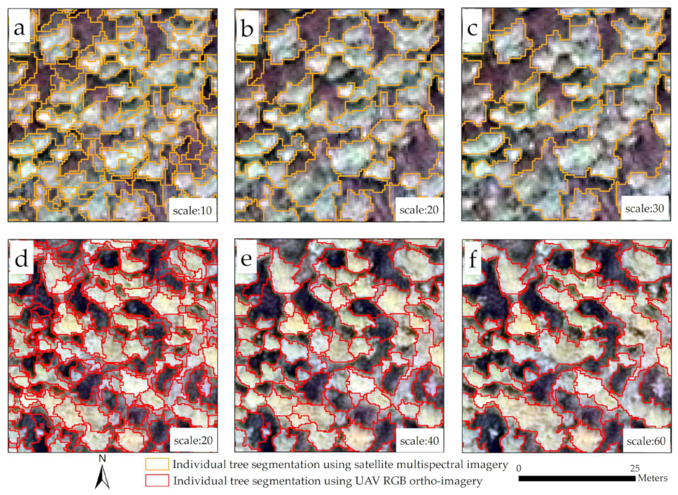
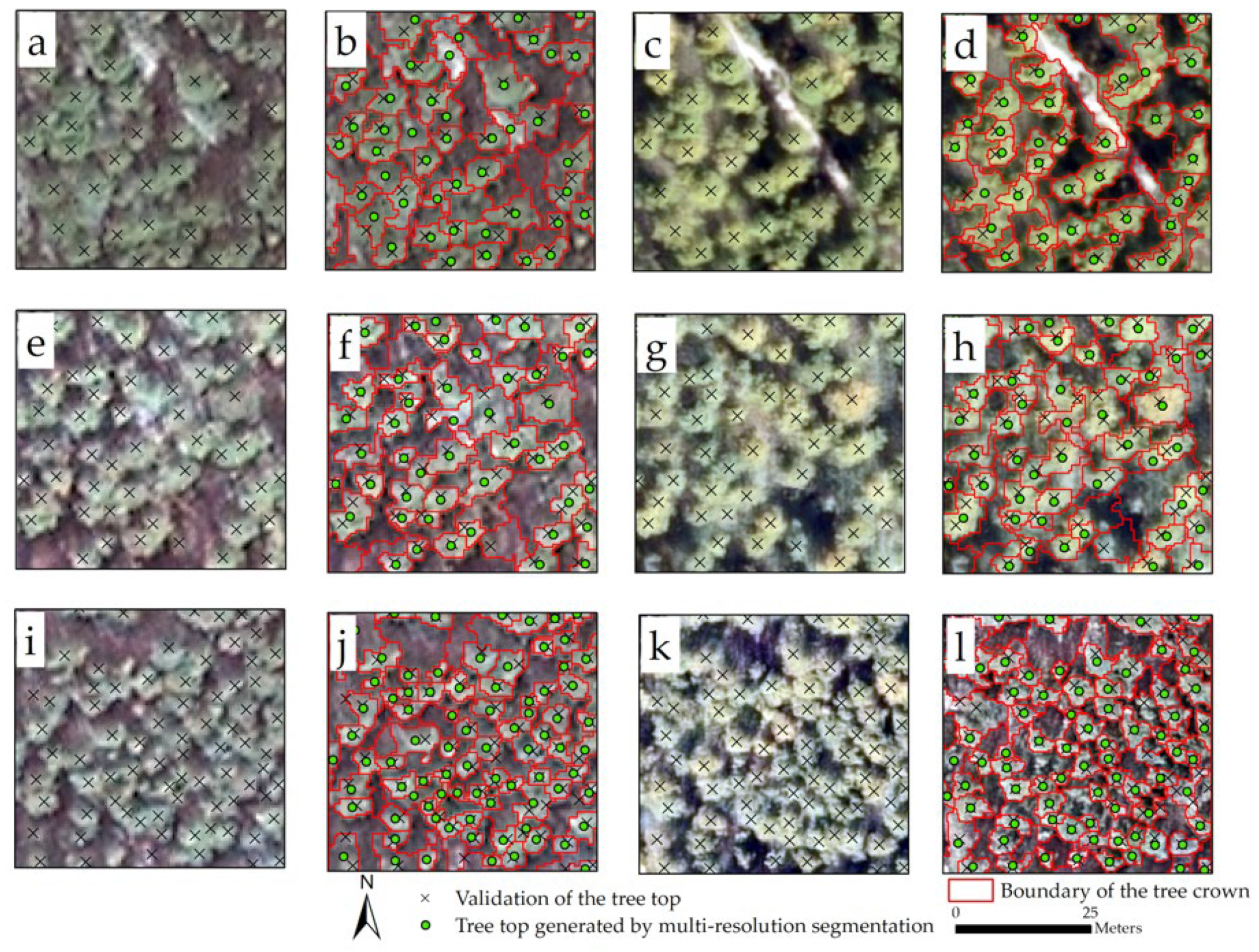
3.1. Individual Tree Segmentation

As shown in Figure 5, the results showed that when the scale factor was 20, the segmented vector layer could be well matched to each tree crown from the multispectral imagery. However, when the scale factor was 10, over-segmentation occurred, with a tree crown being divided into two or more vector layers; when the scale factor was 30, part of the crowns faced under-segmentation. For UAV RGB imagery, the best segmentation performance was obtained when the scale factor was 40. However, when the scale factors were 20 or 60, the individual tree segmentation results could not be well matched to the tree canopy.
As shown in Table 5 and Figure 6, the object-oriented MRS algorithm performed well in the forests with different stand densities (low, middle and high) and had an average overall accuracy greater than 70% (Table 4). For the satellite multispectral imagery, the MRS algorithm had the best detection rate (68.3%) and F1 score (74.7%) in the forests with low density. Under high-density forests, the detection rate of trees was 62.8% and the F1 score was 72.6%. In the middle-density forests, the detection rate of trees was 59.6% and the F1 score was 71.3%. For the UAV high-resolution RGB imagery, the MRS algorithm had the best detection rate (73.1%) and F1 score (79.2%) in the forests with middle density. Under low-density forests, the detection rate of trees was 65.9% and the F1 score was 76.1%. In high-density forests, the detection rate of trees was 66.7% and the F1 score was 75.4%.
The performances of individual tree segmentation using multispectral imagery and high-resolution RGB imagery are shown in Table 6, with the average overall accuracy above 65%. For satellite multispectral imagery, the detection rate of trees was 60.7%, the precision was 75.0% and the F1 score was 67.1%. For the UAV high-resolution RGB imagery, the detection rate of trees was 70.7%, the precision was 74.1% and the F1 score was 72.4%.

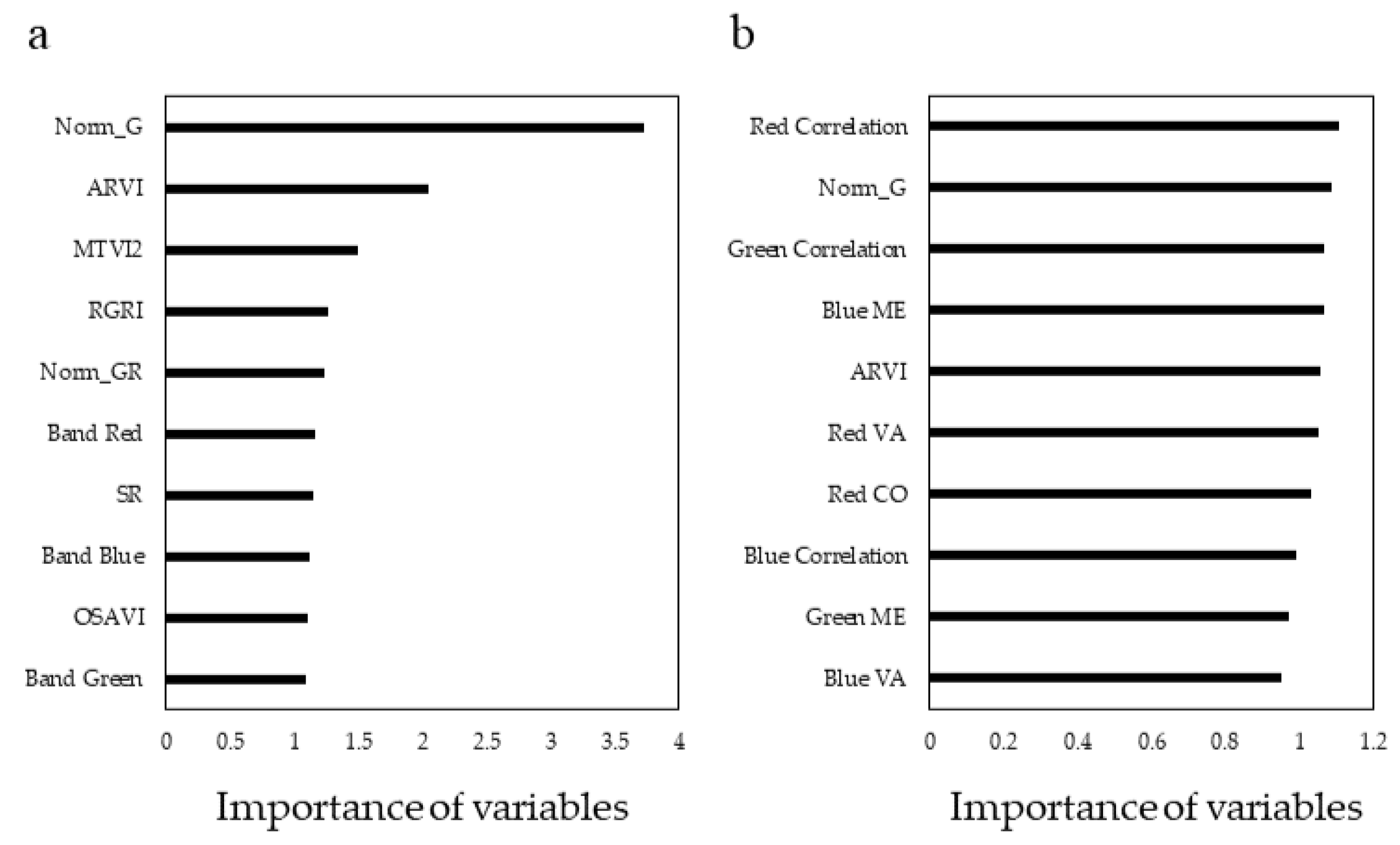
3.2. Feature Optimization and Analysis

The importance analysis of metrics showed that normalized greenness (Norm_G), atmospherically resistant vegetation index (ARVI) and modified triangular vegetation index 2 (MTVI2) of spectral indices were most important for the dominant tree species classification (Figure 7a). With the addition of texture metrics, the contrast of the red band (red correlation), the normalized greenness (Norm_G), and the contrast of the green band (green correlation) ranked in the top three of the ten most important metrics (Figure 7b).

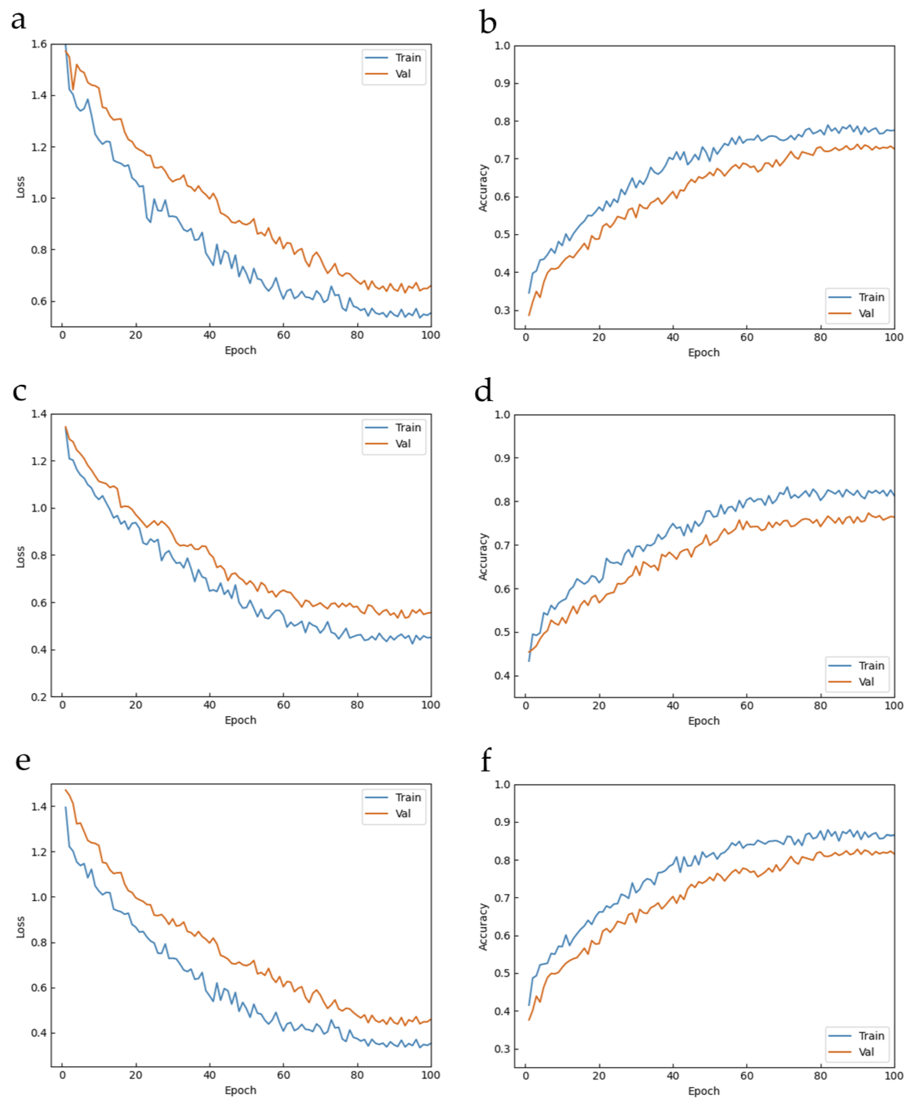
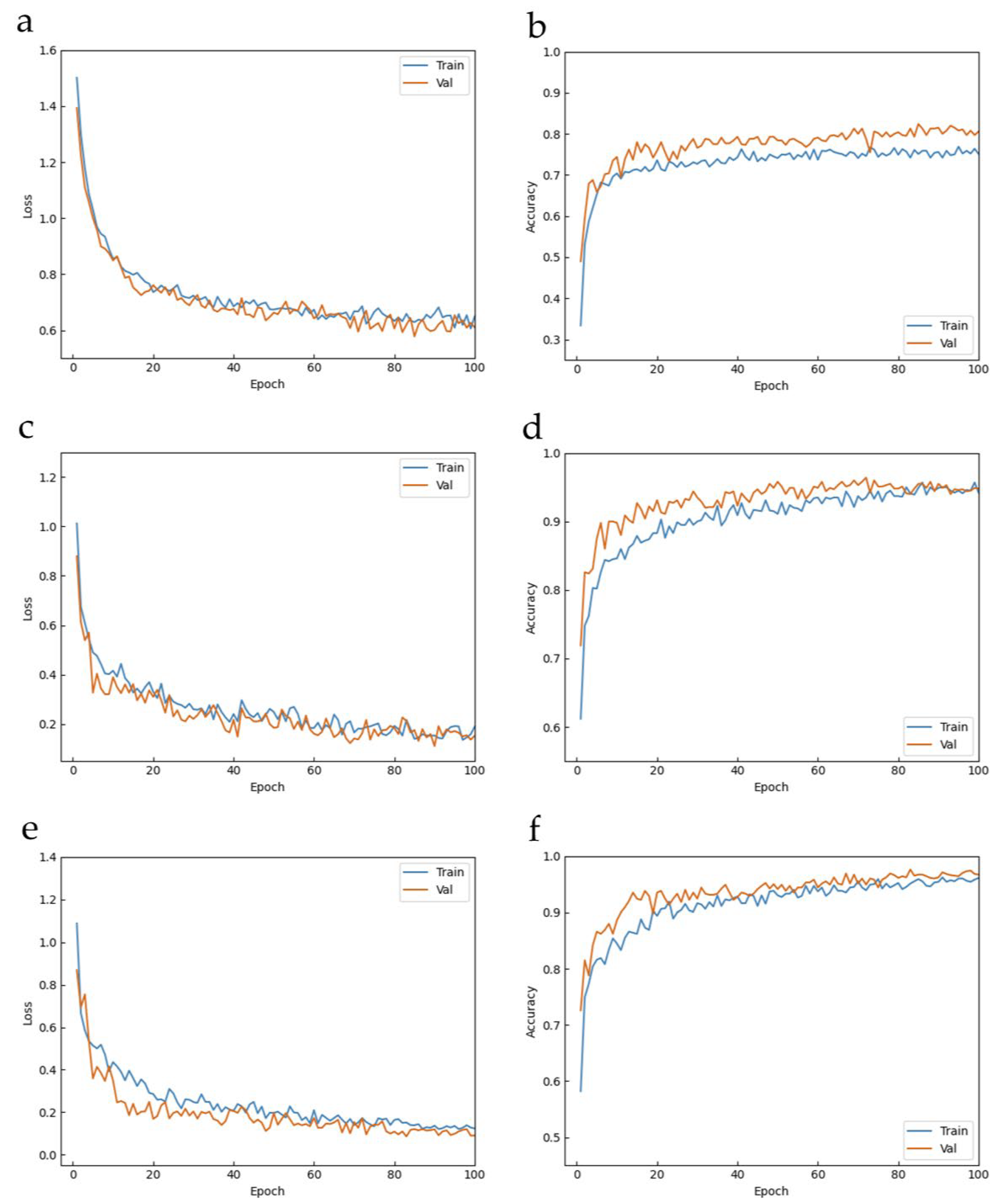
3.3. Training of Deep Learning Networks

In order to compare the classification performances of deep learning networks on different data sources, the satellite multispectral imagery (SV) sample dataset, the multispectral imagery and high-resolution RGB imagery post-stacked image (SVRGB) sample dataset were used to train the deep learning network classifier. For the SV sample dataset, the training processes of the lightweight network MobileNetV2, the residual network ResNet34 and the dense network DesnseNet121 are shown in Figure 8. The blue curve represented the changes in loss value and accuracy in the training samples, and the orange curve represented the changes in loss value and accuracy in the validation samples. Figure 8a shows that the loss values of the lightweight network MobileNetV2 remained stable after 80 epochs. The changes in accuracy also embodied a similar trend in Figure 8b. Figure 8c,d show that the changes in loss value and accuracy in the residual network ResNet34 tended to steady after 70 epochs. Figure 8e,f show that the changes in training loss value and accuracy in the dense network DenseNet121 showed a similar trend to that of the lightweight network MobileNetV2, which stabilized after 80 epochs of iteration.
Similar to the SV sample dataset, three deep learning networks were trained with the SVRGB sample dataset. The overall convergence of this sample dataset was faster than that of the SV sample dataset. As shown in Figure 9a,c, the loss values of the lightweight network MobileNetV2 and the residual network ResNet34 became stable after 60 epochs. In Figure 9b,d, the changes in accuracy remained steady after 60 epochs. The changes in training loss value and accuracy in the dense network DenseNet121 remained stable after 70 epochs, as shown in Figure 9e,f.

3.4. Accuracy Assessment

Table 7 shows the confusion matrix of five dominant tree species classification using the random forest algorithm combined with two groups of metrics. For spectral metrics, the overall accuracy of the dominant tree species classification was 60.00%, and the Kappa accuracy was 47.80%. For the combination of spectral and texture metrics, the overall accuracy of the dominant tree species classification was 64.44%, and the Kappa accuracy was 53.61%. The dominant tree species classification accuracy of using two groups of metrics improved successively, indicating that texture metrics had a positive impact on the dominant tree species classification (OA and Kappa accuracy increased by 4.44% and 5.81%, respectively). Among the five dominant tree species classifications, using the combination of spectral and texture metrics had the best performance (OA was 64.44%, Kappa accuracy was 53.61%).
Table 8 and Table 9 show the confusion matrix of five dominant tree species classifications using the three deep learning networks based on SV and SVRGB sample datasets, respectively. For the SV sample dataset, the average overall accuracy of the three deep learning networks was over than 70%. Dense network DenseNet121 had the highest overall accuracy (OA = 81.11%, Kappa accuracy = 75.53%). The overall accuracy of residual network ResNet34 was followed (OA = 78.89%, Kappa accuracy = 72.86%). Lightweight network MobileNetV2 had the lowest overall accuracy (OA = 71.11%, Kappa accuracy = 63.01%). For the SVRGB sample dataset, the average overall accuracy of the three deep learning networks was more than 80%. Among them, the overall accuracy of dense network DenseNet121 was 94.44%, and the Kappa accuracy was 92.79%, which showed the best classification performance. The overall accuracy of residual network ResNet34 was 91.11%, and the Kappa accuracy was 88.49%, whereas the overall accuracy of lightweight network MobileNetV2 was 82.22%, and the Kappa accuracy was 77.09%. Compared with the SV sample dataset, the average overall accuracy of dominant tree species classification based on the SVRGB sample dataset was improved by 11.11–13.33%.
Therefore, the overall accuracy of the dominant tree species classification of the three deep learning networks (OA = 71.11–94.44%) was higher than that of the random forest algorithm (OA = 60.00–64.44%). Among them, dense network DenseNet121 had the highest overall accuracy (OA = 81.11–94.44%).

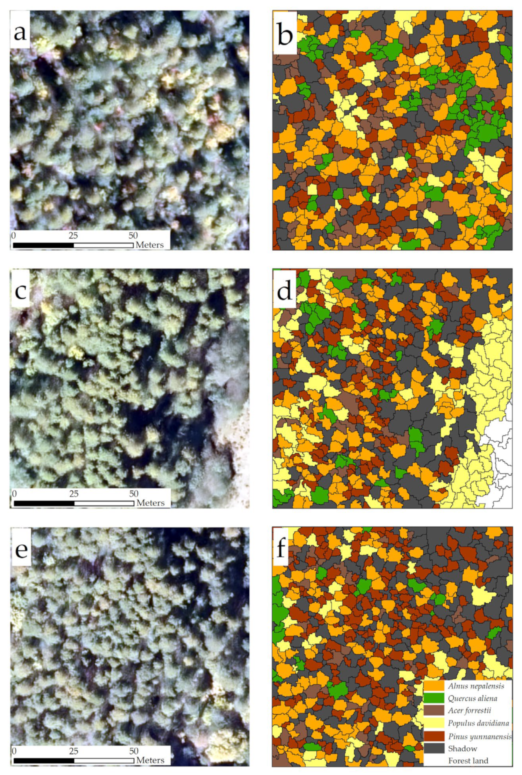
3.5. Mapping of Five Dominant Tree Species

In this paper, the best deep learning network (dense network DenseNet121) was applied to the remote sensing images of individual trees to predict the dominant tree species. It took about 0.5 s to predict each individual tree remote sensing image and obtained the tree species type of the image. Figure 10 shows the mapping of five dominant tree species classifications in three plots (100 × 100 m). In general, Yunnan pine and Nepal alder tree species were dominant in distribution and quantity. In plot 1, the distribution of Nepal alder (A.N.) tree species was more extensive, and the distribution of Oriental white oak (Q.A.) tree species was more concentrated. In plot 2, the number of Yunnan pine (P.Y.) tree species was similar to that of Nepal alder, while aspen (P.D.) tree species were mainly distributed in the eastern of the plot. In plot 3, the number of Nepal alder tree species was the highest and widely distributed. The number of Yunnan pine tree species was second and concentrated in the southwest of the plot.

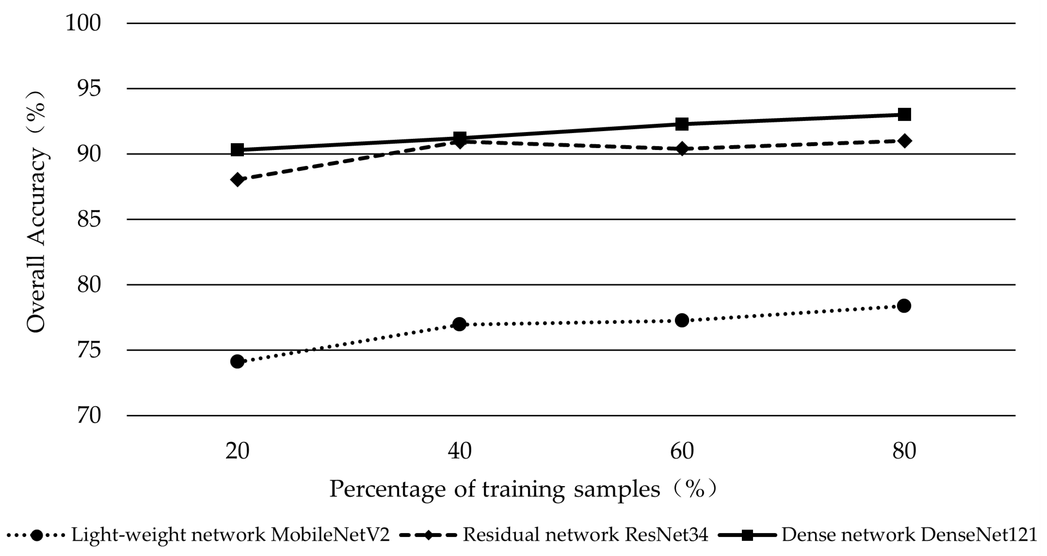
3.6. Effects of the Number of Training Samples on the Classification Performance of Three Deep Learning Networks

The number of training samples has little effect on the overall accuracy of dominant tree species classification using three deep learning networks, as shown in Figure 11. When the number of training samples varied by 20–80% of the total samples of each dominant tree species (the interval was 20%), the overall accuracy of the dominant tree species classification using three deep learning networks changed slightly (the change in OA was 2.69–4.28%). For lightweight network MobileNetV2, the overall accuracy of the dominant tree species classification was 74.09–78.37%. For the residual network ResNet34, the overall accuracy of the dominant tree species classification was 88.05–91.02%. For dense network DenseNet121, the overall accuracy of the dominant tree species classification was 90.32–93.01%.

4. Discussion

4.1. Influence of Different Data Sources on Individual Tree Segmentation

In this study, UAV RGB imagery and satellite multispectral imagery were applied for individual tree segmentation. Compared with the multispectral imagery, the individual tree segmentation accuracy of RGB imagery was higher. The reason is that RGB imagery has higher spatial resolution and clearer canopy boundaries. The lower the spatial resolution, the larger the range of ground objects contained in one pixel, thus potentially interfering with the segmentation of the target object [68]. Moreover, high-resolution RGB images have abundant texture information of tree crown edges, which can be used to accurately extract individual tree crowns [28,69]. Zhou et al. [70] segmented individual trees from high-resolution RGB images, reaching a better segmentation accuracy. However, the complex stand structure, high canopy density and high stand density in natural forests adversely affected the individual tree segmentation. In this paper, although our tree species classification accuracy was high, the individual tree segmentation accuracy was relatively low. It is relatively difficult to segment individual trees in complex stands, which has also been confirmed by previous studies. Xu et al. [35] used three methods to segment individual trees in subtropical natural forests and classified eight types of dominant tree species. The accuracy of the advanced multiresolution segmentation method was highest (F1 score = 82.5%), and the image-based multiresolution segmentation method exhibited the lowest accuracy (F1 score = 78.6%), which is similar to the results (F1 score = 72.4%) obtained in this paper by using RGB images for individual tree segmentation. Zhong et al. [71] used LiDAR point cloud and hyperspectral images for individual tree segmentation in natural forests, and the total accuracy was 84.6%. Compared with our individual tree segmentation results, this accuracy was higher. However, the LiDAR point cloud provides three-dimensional information of the forest canopy structure [72], which can be better used for individual tree segmentation. The data source of this study was two-dimensional images, which do not have this advantage in the process of individual tree segmentation. After the individual tree segmentation was completed, we optimized the segmentation results using a splitting and merging method to match the tree crowns. Although the accuracy of individual tree segmentation in this study was relatively low, the classification accuracy was improved by using the optimized crown boundaries. There is a certain risk, but this risk could be acceptable considering the characteristics of natural forests, such as complex stands and extremely high canopy density. In the future, better methods and data are needed to improve the accuracy of individual tree segmentation in complex stands, so as to provide guidance for forest application.

4.2. Performance of Deep Learning Networks and Effect of Texture metrics on Tree Species Classification

Since the combination of multispectral and RGB data could provide not only spectral information but also texture metrics of the forests, the dominant tree species classification showed a higher accuracy. Previous studies have shown that the combination of many metrics generally showed higher accuracy for dominant tree species classification [73,74]. Gini et al. used texture metrics to improve classification accuracy, and they proved that the use of texture increased OA by 20% [75]. In this study, the random forest algorithm and three deep learning networks were used to classify five dominant tree species. For the random forest algorithm, the addition of texture metrics improved the overall accuracy of dominant tree species classification (the OA was increased by 4.44%). This result was consistent with the conclusion of previous studies. This result occurred because the addition of texture features makes the description of tree species more comprehensive, and the algorithm can identify more features related to the target tree species during classification, thereby improving the classification accuracy. For the deep learning networks, the combination of UAV high-resolution RGB imagery and satellite multispectral imagery enabled the models to learn the features from forest edge and texture, and, thus, the overall accuracy of dominant tree species classification was also improved (the OA was increased by 11.11–13.33%).
In the past, there have been studies using deep learning networks combined with multi-source remote sensing data to improve the overall accuracy of dominant tree species classification [67,76]. However, most previous studies applied deep learning networks to the forests with relatively simple structures. Here, we explored the potential of deep learning networks for the classification of dominant tree species in subtropical natural forests. The result showed that the overall accuracy of dominant tree species classification using the three deep learning networks was higher than that of the random forest algorithm. Previous studies have also proved this point. Onishi et al. [42] used a convolutional neural network (CNN) and SVM algorithm to classify seven classes, and the classification accuracy of CNN was 5.8–13.1% higher than SVM. Zhang et al. [43] used three convolutional neural networks (CNNs) and two machine learning (ML) algorithms to classify tree species; the classification accuracy of CNNs was higher than 70%, while that of ML algorithms was less than 70%. Among the three deep learning networks, dense network had the best performance (81.11–94.44%). The tree species dataset has more complex features, and the convolutional layers in the dense network structure are densely connected with each other, which is more suitable for extracting high-level features. In this paper, three deep learning networks were combined with multi-source remote sensing data to classify five dominant tree species in subtropical natural forests. Compared with the random forest algorithm, the deep learning networks had the potential to identify dominant tree species in subtropical natural forests. However, since the study area selected for tree species classification is only three plots, it is still necessary to explore the large-scale tree species classification.

4.3. Effect of Variation in the Number of Training Samples on Classification Accuracy

Although the variation in training samples had little effect on the overall accuracy of dominant tree species classification using the three deep learning networks, the increased number of training samples had a positive impact on the dominant tree species classification. Hartling et al. divided the total samples into several proportions (10%, 30%, 50% and 70%) to train DenseNet network and found that the overall accuracy of dominant tree species classification increased when the number of samples increased [67]. In this paper, with the increased number of training samples, the overall accuracy of the dominant tree species classification was also improved (the OA was increased by 2.69–4.28%). Furthermore, among the three deep learning networks, the dense network DenseNet121 outperformed the other two models, indicating that it was able to learn deeper information from the sample dataset and, therefore, had strong robustness to the training samples.

5. Conclusions

In this paper, UAV high-resolution RGB imagery and satellite multispectral imagery were obtained, combined with the three deep learning networks and random forest algorithm to identify five dominant tree species in the subtropical natural forest of northwest Yunnan province of China. It was preliminarily confirmed that the deep learning network can be combined with multi-source remote sensing data for the classification of dominant tree species in natural forests. In addition, individual tree segmentation was carried out in natural forests with different stand densities, indicating that the objected-oriented MRS method can be applied to individual tree extraction in natural forests. We found that the individual tree segmentation of UAV high-resolution RGB imagery was better than that of satellite multispectral imagery. A total of 12 spectral indices and 7 texture metrics were extracted from the multispectral imagery and UAV RGB imagery, and the top 10 metrics were selected via the permutation-based importance based on the RF algorithm. In general, Norm_G, ARVI, MTVI2, red correlation and green correlation are the most important metrics in the classification of dominant tree species. Additionally, we found that the overall accuracy of dominant tree species classification using three deep learning networks was higher than that of the random forest algorithm. The addition of texture metrics improved the overall accuracy of dominant tree species classification. For the three deep learning networks, the changes in overall accuracy of dominant tree species classification influenced by the number of training samples were minor, and the classification accuracy of the dense network was higher than that of the other two deep learning networks. This study demonstrated that deep learning networks have the potential to classify dominant tree species in natural forests. However, to further explore their robustness, deep learning networks need to be tested in other study areas and more tree species types.

Author Contributions

Conceptualization, L.C.; methodology, X.C. and X.S.; software, X.C.; validation, X.C. and X.S.; formal analysis, X.C.; writing—original draft preparation, X.C.; writing—review and editing, X.C., X.S. and L.C.; visualization, X.C.; supervision, L.C.; funding acquisition, L.C. All authors have read and agreed to the published version of the manuscript.

Funding

This research was funded by the National Natural Science Foundation of China (31922055) and the Priority Academic Program Development of Jiangsu Higher Education Institutions (PAPD).

Acknowledgments

We gratefully acknowledge staff in Yunnan Baima Snow Mountain National Nature Reserve for assistance with data collection and sharing their rich knowledge and working experience of the local forest ecosystems. The authors also acknowledge the graduate students from the department of forest management at Nanjing Forestry University for providing suggestions for improving this study.

Conflicts of Interest

The authors declare no conflict of interest.

References

  1. Chang, E.H.; Tian, G.L.; Chiu, C.Y. Soil Microbial Communities in Natural and Managed Cloud Montane Forests. Forests 2017, 8, 33. [Google Scholar] [CrossRef]
  2. Liu, Y.Y.; Bian, Z.Q.; Ding, S.Y. Consequences of Spatial Heterogeneity of Forest Landscape on Ecosystem Water Conservation Service in the Yi River Watershed in Central China. Sustainability 2020, 12, 1170. [Google Scholar] [CrossRef]
  3. Zald, H.S.J.; Spies, T.A.; Harmon, M.E.; Twery, M.J. Forest Carbon Calculators: A Review for Managers, Policymakers, and Educators. J. For. 2016, 114, 134–143. [Google Scholar] [CrossRef]
  4. Brockerhoff, E.G.; Barbaro, L.; Castagneyrol, B.; Forrester, D.I.; Gardiner, B.; González-Olabarria, J.R.; Lyver, P.O.B.; Meurisse, N.; Oxbrough, A.; Taki, H.; et al. Forest biodiversity, ecosystem functioning and the provision of ecosystem services. Biodivers. Conserv. 2017, 26, 3005–3035. [Google Scholar] [CrossRef]
  5. Hartley, M.J. Rationale and methods for conserving biodiversity in plantation forests. For. Ecol. Manag. 2002, 155, 81–95. [Google Scholar] [CrossRef]
  6. Hooper, D.U.; Chapin, F.S.; Ewel, J.J.; Hector, A.; Inchausti, P.; Lavorel, S.; Lawton, J.H.; Lodge, D.M.; Loreau, M.; Naeem, S.; et al. Effects of biodiversity on ecosystem functioning: A consensus of current knowledge. Ecol. Monogr. 2005, 75, 3–35. [Google Scholar] [CrossRef]
  7. Modzelewska, A.; Fassnacht, F.E.; Stereńczak, K. Tree species identification within an extensive forest area with diverse management regimes using airborne hyperspectral data. Int. J. Appl. Earth Obs. Geoinf. 2020, 84, 101960. [Google Scholar] [CrossRef]
  8. Piiroinen, R.; Fassnacht, F.E.; Heiskanen, J.; Maeda, E.; Mack, B.; Pellikka, P. Invasive tree species detection in the Eastern Arc Mountains biodiversity hotspot using one class classification. Remote Sens. Environ. 2018, 218, 119–131. [Google Scholar] [CrossRef]
  9. Jonsson, M.; Bengtsson, J.; Gamfeldt, L.; Moen, J.; Snäll, T. Levels of forest ecosystem services depend on specific mixtures of commercial tree species. Nat. Plants 2019, 5, 141–147. [Google Scholar] [CrossRef]
  10. Ali, A.; Mattsson, E. Disentangling the effects of species diversity, and intraspecific and interspecific tree size variation on aboveground biomass in dry zone homegarden agroforestry systems. Sci. Total Environ. 2017, 598, 38–48. [Google Scholar] [CrossRef]
  11. Fichtner, A.; Hardtle, W.; Li, Y.; Bruelheide, H.; Kunz, M.; von Oheimb, G. From competition to facilitation: How tree species respond to neighbourhood diversity. Ecol. Lett. 2017, 20, 892–900. [Google Scholar] [CrossRef] [PubMed]
  12. Dalponte, M.; Bruzzone, L.; Gianelle, D. Fusion of hyperspectral and LIDAR remote sensing data for classification of complex forest areas. IEEE Trans. Geosci. Remote Sens. 2008, 46, 1416–1427. [Google Scholar] [CrossRef]
  13. Ghosh, A.; Fassnacht, F.E.; Joshi, P.K.; Koch, B. A framework for mapping tree species combining hyperspectral and LiDAR data: Role of selected classifiers and sensor across three spatial scales. Int. J. Appl. Earth Obs. Geoinf. 2014, 26, 49–63. [Google Scholar] [CrossRef]
  14. Immitzer, M.; Atzberger, C.; Koukal, T. Tree Species Classification with Random Forest Using Very High Spatial Resolution 8-Band WorldView-2 Satellite Data. Remote Sens. 2012, 4, 2661–2693. [Google Scholar] [CrossRef]
  15. McRoberts, R.E.; Tomppo, E.O. Remote sensing support for national forest inventories. Remote Sens. Environ. 2007, 110, 412–419. [Google Scholar] [CrossRef]
  16. Feret, J.-B.; Asner, G.P.; Sensing, R. Tree Species Discrimination in Tropical Forests Using Airborne Imaging Spectroscopy. IEEE Trans. Geosci. Remote Sens. 2013, 51, 73–84. [Google Scholar] [CrossRef]
  17. Li, J.L.; Hu, B.X.; Noland, T.L. Classification of tree species based on structural features derived from high density LiDAR data. Agric. For. Meteorol. 2013, 171, 104–114. [Google Scholar] [CrossRef]
  18. Bhardwaj, A.; Sam, L.; Akanksha; Martin-Torres, F.J.; Kumar, R. UAVs as remote sensing platform in glaciology: Present applications and future prospects. Remote Sens. Environ. 2016, 175, 196–204. [Google Scholar] [CrossRef]
  19. Yu, Y.; Li, M.; Fu, Y. Forest type identification by random forest classification combined with SPOT and multitemporal SAR data. J. For. Res. 2018, 29, 1407–1414. [Google Scholar] [CrossRef]
  20. Fassnacht, F.E.; Latifi, H.; Stereńczak, K.; Modzelewska, A.; Lefsky, M.; Waser, L.T.; Straub, C.; Ghosh, A. Review of studies on tree species classification from remotely sensed data. Remote Sens. Environ. 2016, 186, 64–87. [Google Scholar] [CrossRef]
  21. Cho, M.A.; Malahlela, O.E.; Ramoelo, A.J. Assessing the utility WorldView-2 imagery for tree species mapping in South African subtropical humid forest and the conservation implications: Dukuduku forest patch as case study. Int. J. Appl. Earth Obs. Geoinf. 2015, 38, 349–357. [Google Scholar] [CrossRef]
  22. Johansen, K.; Phinn, S. Mapping indicators of riparian vegetation health using IKONOS and Landsat-7 ETM+ image data in Australian tropical savannas. In Proceedings of the IGARSS 2004, 2004 IEEE International Geoscience and Remote Sensing Symposium, Anchorage, AK, USA, 20–24 September 2004; Volume 1553, pp. 1559–1562. [Google Scholar]
  23. Mallinis, G.; Koutsias, N.; Tsakiri-Strati, M.; Karteris, M. Object-based classification using Quickbird imagery for delineating forest vegetation polygons in a Mediterranean test site. ISPRS J. Photogramm. Remote Sens. 2008, 63, 237–250. [Google Scholar] [CrossRef]
  24. Deur, M.; Gasparovic, M.; Balenović, I. Tree Species Classification in Mixed Deciduous Forests Using Very High Spatial Resolution Satellite Imagery and Machine Learning Methods. Remote Sens. 2020, 12, 3926. [Google Scholar] [CrossRef]
  25. Ferreira, M.P.; Wagner, F.H.; Aragão, L.E.O.C.; Shimabukuro, Y.E.; de Souza Filho, C.R. Tree species classification in tropical forests using visible to shortwave infrared WorldView-3 images and texture analysis. ISPRS J. Photogramm. Remote Sens. 2019, 149, 119–131. [Google Scholar] [CrossRef]
  26. Zhang, J.; Hu, J.B.; Lian, J.Y.; Fan, Z.J.; Ouyang, X.J.; Ye, W.H. Seeing the forest from drones: Testing the potential of lightweight drones as a tool for long-term forest monitoring. Biol. Conserv. 2016, 198, 60–69. [Google Scholar] [CrossRef]
  27. Reis, B.P.; Martins, S.V.; Fernandes, E.I.; Sarcinelli, T.S.; Gleriani, J.M.; Leite, H.G.; Halassy, M. Forest restoration monitoring through digital processing of high resolution images. Ecol. Eng. 2019, 127, 178–186. [Google Scholar] [CrossRef]
  28. Dash, J.P.; Watt, M.S.; Pearse, G.D.; Heaphy, M.; Dungey, H.S. Assessing very high resolution UAV imagery for monitoring forest health during a simulated disease outbreak. ISPRS J. Photogramm. Remote Sens. 2017, 131, 1–14. [Google Scholar] [CrossRef]
  29. Nuijten, R.; Coops, N.; Goodbody, T.; Pelletier, G. Examining the Multi-Seasonal Consistency of Individual Tree Segmentation on Deciduous Stands Using Digital Aerial Photogrammetry (DAP) and Unmanned Aerial Systems (UAS). Remote Sens. 2019, 11, 739. [Google Scholar] [CrossRef]
  30. Chen, L.; Jia, J.; Wang, H.J. An overview of applying high resolution remote sensing to natural resources survey. Remote Sens. Nat. Resour. 2019, 31, 1–7. [Google Scholar]
  31. Marques, P.; Pádua, L.; Adão, T.; Hruška, J.; Peres, E.; Sousa, A.; Sousa, J.J. UAV-Based Automatic Detection and Monitoring of Chestnut Trees. Remote Sens. 2019, 11, 855. [Google Scholar] [CrossRef]
  32. Ryherd, S.; Woodcock, C. Combining Spectral and Texture Data in the Segmentation of Remotely Sensed Images. Photogramm. Eng. Remote Sens. 1996, 62, 181–194. [Google Scholar]
  33. Blaschke, T. Object-based contextual image classification built on image segmentation. In Proceedings of the IEEE Workshop on Advances in Techniques for Analysis of Remotely Sensed Data, Greenbelt, MD, USA, 27–28 October 2003; pp. 113–119. [Google Scholar]
  34. Elisabeth, A.A. The Importance of Scale in Object-based Mapping of Vegetation Parameters with Hyperspectral Imagery. Photogramm. Eng. Remote Sens. 2007, 73, 905–912. [Google Scholar] [CrossRef]
  35. Xu, Z.; Shen, X.; Cao, L.; Coops, N.C.; Goodbody, T.R.H.; Zhong, T.; Zhao, W.; Sun, Q.; Ba, S.; Zhang, Z.; et al. Tree species classification using UAS-based digital aerial photogrammetry point clouds and multispectral imageries in subtropical natural forests. Int. J. Appl. Earth Obs. Geoinf. 2020, 92, 102173. [Google Scholar] [CrossRef]
  36. Kattenborn, T.; Leitloff, J.; Schiefer, F.; Hinz, S. Review on Convolutional Neural Networks (CNN) in vegetation remote sensing. Isprs J. Photogramm. Remote Sens. 2021, 173, 24–49. [Google Scholar] [CrossRef]
  37. Schiefer, F.; Kattenborn, T.; Frick, A.; Frey, J.; Schall, P.; Koch, B.; Schmidtlein, S. Mapping forest tree species in high resolution UAV-based RGB-imagery by means of convolutional neural networks. Isprs J. Photogramm. Remote Sens. 2020, 170, 205–215. [Google Scholar] [CrossRef]
  38. Natesan, S.; Armenakis, C.; Vepakomma, U. Resnet-Based Tree Species Classification Using Uav Images. Int. Arch. Photogramm. Remote Sens. Spat. Inf. Sci. 2019, XLII-2/W13, 475–481. [Google Scholar] [CrossRef]
  39. Guo, X.; Li, H.; Jing, L.; Wang, P. Individual Tree Species Classification Based on Convolutional Neural Networks and Multitemporal High-Resolution Remote Sensing Images. Sensors 2022, 22, 3157. [Google Scholar] [CrossRef]
  40. Yan, S.J.; Jing, L.H.; Wang, H. A New Individual Tree Species Recognition Method Based on a Convolutional Neural Network and High-Spatial Resolution Remote Sensing Imagery. Remote Sens. 2021, 13, 479. [Google Scholar] [CrossRef]
  41. Xi, Z.; Hopkinson, C.; Rood, S.B.; Peddle, D.R. See the forest and the trees: Effective machine and deep learning algorithms for wood filtering and tree species classification from terrestrial laser scanning. ISPRS J. Photogramm. Remote Sens. 2020, 168, 1–16. [Google Scholar] [CrossRef]
  42. Onishi, M.; Ise, T. Explainable identification and mapping of trees using UAV RGB image and deep learning. Sci. Rep. 2021, 11, 903. [Google Scholar] [CrossRef]
  43. Zhang, C.; Xia, K.; Feng, H.; Yang, Y.; Du, X. Tree species classification using deep learning and RGB optical images obtained by an unmanned aerial vehicle. J. For. Res. 2020, 32, 1879–1888. [Google Scholar] [CrossRef]
  44. Li, H.; Jing, L.; Tang, Y.; Ding, H. An Improved Pansharpening Method for Misaligned Panchromatic and Multispectral Data. Sensors 2018, 18, 557. [Google Scholar] [CrossRef] [PubMed]
  45. Lim, W.; Choi, K.; Cho, W.; Chang, B.; Ko, D.W. Efficient dead pine tree detecting method in the Forest damaged by pine wood nematode (Bursaphelenchus xylophilus) through utilizing unmanned aerial vehicles and deep learning-based object detection techniques. For. Sci. Technol. 2022, 18, 36–43. [Google Scholar] [CrossRef]
  46. Long, Y.; Gong, Y.; Xiao, Z.; Liu, Q.J. Accurate Object Localization in Remote Sensing Images Based on Convolutional Neural Networks. IEEE Trans. Geosci. Remote Sens. 2017, 55, 2486–2498. [Google Scholar] [CrossRef]
  47. Cheng, G.; Zhou, P.; Han, J. Learning Rotation-Invariant Convolutional Neural Networks for Object Detection in VHR Optical Remote Sensing Images. IEEE Trans. Geosci. Remote Sens. 2016, 54, 7405–7415. [Google Scholar] [CrossRef]
  48. Zhang, W.; Sun, X.; Fu, K.; Wang, C.; Wang, H. Object Detection in High-Resolution Remote Sensing Images Using Rotation Invariant Parts Based Model. IEEE Geosci. Remote Sens. Lett. 2014, 11, 74–78. [Google Scholar] [CrossRef]
  49. Ju, C.-H.; Tian, Y.-C.; Yao, X.; Cao, W.-X.; Zhu, Y.; Hannaway, D. Estimating Leaf Chlorophyll Content Using Red Edge Parameters. Pedosphere 2010, 20, 633–644. [Google Scholar] [CrossRef]
  50. Kaufman, Y.J.; Tanré, D. Strategy for direct and indirect methods for correcting the aerosol effect on remote sensing: From AVHRR to EOS-MODIS. Remote Sens. Environ. 1996, 55, 65–79. [Google Scholar] [CrossRef]
  51. Verstraete, M.M.; Pinty, B. Designing optimal spectral indexes for remote sensing applications. IEEE Trans. Geosci. Remote Sens. 1996, 34, 1254–1265. [Google Scholar] [CrossRef]
  52. Haboudane, D.; Miller, J.R.; Pattey, E.; Zarco-Tejada, P.J.; Strachan, I.B. Hyperspectral vegetation indices and novel algorithms for predicting green LAI of crop canopies: Modeling and validation in the context of precision agriculture. Remote Sens. Environ. 2004, 90, 337–352. [Google Scholar] [CrossRef]
  53. Peñuelas, J.; Gamon, J.A.; Griffin, K.L.; Field, C.B. Assessing community type, plant biomass, pigment composition, and photosynthetic efficiency of aquatic vegetation from spectral reflectance. Remote Sens. Environ. 1993, 46, 110–118. [Google Scholar] [CrossRef]
  54. Darvishzadeh, R.; Atzberger, C.; Skidmore, A.K.; Abkar, A.A. Leaf Area Index derivation from hyperspectral vegetation indicesand the red edge position. Int. J. Remote Sens. 2009, 30, 6199–6218. [Google Scholar] [CrossRef]
  55. Fraser, R.H.; Sluijs, J.v.d.; Hall, R.J.J. Calibrating Satellite-Based Indices of Burn Severity from UAV-Derived Metrics of a Burned Boreal Forest in NWT, Canada. Remote Sens. 2017, 9, 279. [Google Scholar] [CrossRef]
  56. Yuan, J.; Niu, Z.; Fu, W. Model simulation for sensitivity of hyperspectral indices to LAI, leaf chlorophyll, and internal structure parameter. In Proceedings of the Geoinformatics 2007: Remotely Sensed Data and Information, Nanjing, China, 8 August 2007. [Google Scholar] [CrossRef]
  57. Gamon, J.; Surfus, J. Assessing leaf pigment content and activity with a reflectometer. New Phytol. 1999, 143, 105–117. [Google Scholar] [CrossRef]
  58. Breiman, L. Random Forests. Mach. Learn. 2001, 45, 5–32. [Google Scholar] [CrossRef]
  59. Zhu, R.; Zeng, D.; Kosorok, M.R.J. Reinforcement Learning Trees. J. Am. Stat. Assoc. 2015, 110, 1770. [Google Scholar] [CrossRef]
  60. Sandler, M.; Howard, A.; Zhu, M.L.; Zhmoginov, A.; Chen, L.C. MobileNetV2: Inverted Residuals and Linear Bottlenecks. In Proceedings of the 31st IEEE/CVF Conference on Computer Vision and Pattern Recognition (CVPR), Salt Lake City, UT, USA, 18–23 June 2018; pp. 4510–4520. [Google Scholar]
  61. He, K.M.; Zhang, X.Y.; Ren, S.Q.; Sun, J. Deep Residual Learning for Image Recognition. In Proceedings of the 2016 IEEE Conference on Computer Vision and Pattern Recognition (CVPR), Seattle, WA, USA, 27–30 June 2016; pp. 770–778. [Google Scholar]
  62. Huang, G.; Liu, Z.; van der Maaten, L.; Weinberger, K.Q. Densely Connected Convolutional Networks. In Proceedings of the 30th IEEE/CVF Conference on Computer Vision and Pattern Recognition (CVPR), Honolulu, HI, USA, 21–26 July 2016; pp. 2261–2269. [Google Scholar]
  63. Benz, U.C.; Hofmann, P.; Willhauck, G.; Lingenfelder, I.; Heynen, M. Multi-resolution, object-oriented fuzzy analysis of remote sensing data for GIS-ready information. ISPRS J. Photogramm. Remote Sens. 2004, 58, 239–258. [Google Scholar] [CrossRef]
  64. Goutte, C.; Gaussier, E. A Probabilistic Interpretation of Precision, Recall and F-Score, with Implication for Evaluation. In Advances in Information Retrieval, Proceedings of the 27th European Conference on IR Research, ECIR 2005, Santiago de Compostela, Spain,21–23 March 2005; Springer: Berlin/Heidelberg, Germany, 2005; pp. 345–359. [Google Scholar]
  65. Sokolova, M.; Japkowicz, N.; Szpakowicz, S. Beyond Accuracy, F-Score and ROC: A Family of Discriminant Measures for Performance Evaluation. In AI 2006: Advances in Artificial Intelligence, Proceedings of the 19th Australian Joint Conference on Artificial Intelligence, Hobart, Australia, 4–8 December 2006; Springer: Berlin/Heidelberg, Germany, 2006; pp. 1015–1021. [Google Scholar]
  66. Nevalainen, O.; Honkavaara, E.; Tuominen, S.; Viljanen, N.; Hakala, T.; Yu, X.; Hyyppä, J.; Saari, H.; Pölönen, I.; Imai, N.; et al. Individual Tree Detection and Classification with UAV-Based Photogrammetric Point Clouds and Hyperspectral Imaging. Remote Sens. 2017, 9, 185. [Google Scholar] [CrossRef]
  67. Hartling, S.; Sagan, V.; Sidike, P.; Maimaitijiang, M.; Carron, J. Urban Tree Species Classification Using a WorldView-2/3 and LiDAR Data Fusion Approach and Deep Learning. Sensors 2019, 19, 1284. [Google Scholar] [CrossRef]
  68. Wang, X.; Tan, L.; Fan, J. Performance Evaluation of Mangrove Species Classification Based on Multi-Source Remote Sensing Data Using Extremely Randomized Trees in Fucheng Town, Leizhou City, Guangdong Province. Remote Sens. 2023, 15, 1386. [Google Scholar] [CrossRef]
  69. Lisein, J.; Pierrot-Deseilligny, M.; Bonnet, S.; Lejeune, P. A Photogrammetric Workflow for the Creation of a Forest Canopy Height Model from Small Unmanned Aerial System Imagery. Forests 2013, 4, 922–944. [Google Scholar] [CrossRef]
  70. Zhou, X.; Zhang, X. Individual Tree Parameters Estimation for Plantation Forests Based on UAV Oblique Photography. IEEE Access 2020, 8, 96184–96198. [Google Scholar] [CrossRef]
  71. Zhong, H.; Lin, W.S.; Liu, H.R.; Ma, N.; Liu, K.K.; Cao, R.Z.; Wang, T.T.; Ren, Z.Z. Identification of tree species based on the fusion of UAV hyperspectral image and LiDAR data in a coniferous and broad-leaved mixed forest in Northeast China. Front. Plant Sci. 2022, 13, 964769. [Google Scholar] [CrossRef]
  72. Drake, J.B.; Dubayah, R.O.; Knox, R.G.; Clark, D.B.; Blair, J.B. Sensitivity of large-footprint lidar to canopy structure and biomass in a neotropical rainforest. Remote Sens. Environ. 2002, 81, 378–392. [Google Scholar] [CrossRef]
  73. Hartling, S.; Sagan, V.; Maimaitijiang, M. Urban tree species classification using UAV-based multi-sensor data fusion and machine learning. GISci. Remote Sens. 2021, 58, 1–26. [Google Scholar] [CrossRef]
  74. Matsuki, T.; Yokoya, N.; Iwasaki, A. Hyperspectral Tree Species Classification of Japanese Complex Mixed Forest with the Aid of Lidar Data. IEEE J. Sel. Top. Appl. Earth Obs. Remote Sens. 2015, 8, 2177–2187. [Google Scholar] [CrossRef]
  75. Gini, R.; Sona, G.; Ronchetti, G.; Passoni, D.; Pinto, L. Improving Tree Species Classification Using UAS Multispectral Images and Texture Measures. ISPRS Int. J. Geo-Inf. 2018, 7, 315. [Google Scholar] [CrossRef]
  76. Nezami, S.; Khoramshahi, E.; Nevalainen, O.; Pölönen, I.; Honkavaara, E. Tree Species Classification of Drone Hyperspectral and RGB Imagery with Deep Learning Convolutional Neural Networks. Remote Sens. 2020, 12, 1070. [Google Scholar] [CrossRef]
Figure 1. The workflow of dominant tree species classification in subtropical natural forests of northwest Yunnan province using multi-source fine-scale remote sensing data and deep learning network approaches.
Remotesensing 15 02697 g001
Figure 2. Overview of the Gehuaqing (GHQ) study site. (a) Map of Yunnan province and the location of Gehuaqing; (b) UAV high-resolution RGB imagery and spatial distribution of individual trees measured in the field work; (c) high-resolution satellite multispectral imagery of the study site.
Remotesensing 15 02697 g002
Figure 3. Steps for constructing the sample dataset of individual trees. (a) Ortho-imagery of the study area (RGB display); (b) individual tree crown boundaries generated via object-oriented MRS algorithm; (c) individual tree samples obtained from field measurement (the red and green dots are individual trees of Yunnan pine and Oriental white oak); (d) crowns of dominant individual tree species; (e) tree crown images of dominant individual tree species. See Table 1 for short descriptions of the dominant tree species.
Remotesensing 15 02697 g003
Figure 4. Framework of the three deep learning networks. (a) Lightweight network MobileNetV2 framework; (b) residual network ResNet34 framework; (c) dense network DenseNet121 framework.
Remotesensing 15 02697 g004
Figure 5. Sensitivity analysis of individual tree segmentation using object-oriented MRS algorithm (plot size: 50 × 50 m). (ac) MRS segmentation using satellite multispectral imagery (the segmentation scale factors are 10, 20 and 30, respectively); (df) MRS segmentation using UAV RGB imagery (the segmentation scale factors are 20, 40 and 60, respectively).
Remotesensing 15 02697 g005
Figure 6. The multispectral imagery and high-resolution RGB imagery with the positions of individual trees (test data), tree tops and tree crowns were detected via the object-oriented MRS algorithm in the forests with three stand densities (low (N = 41), middle (N = 52) and high (N = 78)). (a,e,i) Multispectral imagery; (b,f,j) individual tree segmentation using the multispectral imagery combined with MRS algorithm in the three plots; (c,g,k) high-resolution RGB imagery; (d,h,l) individual tree segmentation using the high-resolution RGB imagery combined with MRS algorithm in the three plots.
Remotesensing 15 02697 g006
Figure 7. The importance values of the ten most important metrics of the random forest algorithm used for the dominant tree species classification. (a) Dominant tree species classification using spectral indices; (b) dominant tree species classification using spectral and texture metrics. Note: red correlation represents the correlation degree of red band. Red VA represents the variance in the red band; red CO represents the contrast of the red band. See Table 3b for short descriptions of the spectral and texture metrics.
Remotesensing 15 02697 g007
Figure 8. Training processes of the three deep learning networks based on SV sample dataset. (a) Change in loss value in the lightweight network MobileNetV2; (b) change in accuracy in lightweight network MobileNetV2; (c) change in loss value in the residual network ResNet34; (d) change in accuracy in the residual network ResNet34; (e) change in loss value in the dense network DenseNet121; (f) change in accuracy in the dense network DenseNet121.
Remotesensing 15 02697 g008
Figure 9. Training processes of the three deep learning networks based on SVRGB sample dataset. (a) Change in loss value in the light-weight network MobileNetV2; (b) change in accuracy in lightweight network MobileNetV2; (c) change in loss value in the residual network ResNet34; (d) change in accuracy in the residual network ResNet34; (e) change in loss value in the dense network DenseNet121; (f) change in accuracy in the dense network DenseNet121.
Remotesensing 15 02697 g009
Figure 10. Mapping of five dominant tree species classifications in three plots (100 × 100 m). Left: Image after RGB imagery and multispectral imagery stacked (display in RGB); (a,c,e) plot 1, plot 2 and plot 3, respectively. Right: The results of five dominant tree species classifications using dense network DenseNet121; (b,d,f) the five dominant tree species classifications mapping plot 1, plot 2 and plot 3, respectively. See Table 1 for short descriptions of the dominant tree species.
Remotesensing 15 02697 g010
Figure 11. The overall accuracy of three deep learning networks using 20%, 40%, 60% and 80% of the total samples of each dominant tree species based on the SVRGB sample dataset.
Remotesensing 15 02697 g011
Table 1. Summary statistics of the trees measured.
Scientific NameNDBH (cm)Height (m)Crown Width (m)
MeanSDMeanSDMeanSD
Alnus nepalensis (A.N.)11827.8721.0113.106.635.321.91
Quercus aliena (Q.A.)8055.7219.3723.416.076.762.30
Populus davidiana (P.D.)9730.9623.0711.345.565.442.22
Acer forrestii (A.F.)8037.9018.6514.594.936.972.20
Pinus yunnanensis (P.Y.)7538.9117.9522.238.045.311.58
Note: DBH: diameter at breast height (cm); H: height (m); N: number of trees; Alnus nepalensis = A.N.; Quercus aliena = Q.A.; Populus davidiana = P.D.; Acer forrestii = A.F.; Pinus yunnanensis = P.Y.
Table 2. Number of samples of each dominant tree species.
ClassTrainingValidationTotal
A.N.472118590
Q.A.32080400
P.D.38897485
A.F.32080400
P.Y.30075375
Total18004502250
Note: Alnus nepalensis = A.N.; Quercus aliena = Q.A.; Populus davidiana = P.D.; Acer forrestii = A.F.; Pinus yunnanensis = P.Y.
Table 3. Summary of the vegetation indices with respective equations and references.
MetricsEquationReference
Difference Vegetation Index (DVI)ρnir − ρred[49]
Atmospherically Resistant Vegetation Index (ARVI) nir − ρrb)/(ρnir + ρrb), ρrb = ρred – γ × (ρblue − ρred), γ = 0.5[50]
Green Normalized Difference Vegetation Index (GNDVI)nir − ρgreen)/(ρnir + ρgreen)[51]
Modified triangular vegetation index 2 (MTVI2)[1.5 × (1.2 × (ρnir − ρgreen) − 2.5 × (ρred −ρgreen)]/[(2 × ρnir+1)2 – (6 × ρnir – 5 × ρred0.5) – 0.5]0.5[52]
Normalized Difference Vegetation Index (NDVI)nir – ρred)/(ρnir + ρred)[52]
Simple Ration Vegetation Index (SR)ρnirred[53]
Soil Adjusted Vegetation Index (SAVI)1.5 × (ρnir − ρred)/(ρnir + ρred + 0.5)[52]
Ratio Vegetation Index (RVI)ρrednir[54]
Normalized Greenness (Norm G)ρgreen/(ρred + ρgreen+ ρblue)[55]
Normalized Green-Red Ratio (Norm GR)green – ρred)/(ρgreen + ρred)[55]
Optimized Soil Adjusted Vegetation Index (OSAVI)nir – ρred)/(ρnir + ρred + 0.16)[56]
Red Green Ratio Index (RGRI)ρredgreen[57]
Note: the ρblue represents the reflectance of blue band; the ρgreen represents the reflectance of green band; the ρred represents the reflectance of red bands; the ρnir represents the reflectance of near-infrared band.
Table 4. Summary of the texture metrics with respective equations and references.
MetricsEquation
Correlation (CR)CR = i , j = 0 N 1 i · P i , j | i M E j M E V A i V A j |
Contrast (CO)CO = | i , j = 0 N 1 n 2 · P i , j |
Dissimilarity (DI)DI = i , j = 0 N 1 i · P i , j | i j |
Entropy (EN)EN = i , j = 0 N 1 i · P i , j (− ln P i , j )
Homogeneity (HO)HO = i , j = 0 N 1 i · P i , j 1 + i j 2
Mean (ME)ME = i , j = 0 N 1 i · P i , j
Variance (VA)VA = i , j = 0 N 1 i · P i , j ( i M E )
Note: i, j represents the gray scale of image; N represents the gray level of image; Pi,j represents the gray-level co-occurrence matrix.
Table 5. Accuracy assessment of individual tree segmentation in the forests with different stand densities.
DensityNtNoNcr (%)p (%)F1 (%)
Satellite multispectral imagery
Low2813668.382.474.7
Middle3121459.688.671.3
High4929862.885.972.6
UAV high-resolution RGB imagery
Low2714365.990.076.1
Middle3814673.186.479.2
High5226866.786.775.4
Note: r, represents the rate of tree detection; p, represents the detection trees precision; F1, represents the overall accuracy taking both omission and commission in consideration.
Table 6. Accuracy assessment of individual tree segmentation of dominant tree species.
Data SourceNtNoNcr (%)p (%)F1 (%)
Satellite multispectral imagery2731779160.775.067.1
UAV high-resolution RGB imagery31813211170.774.172.4
Note: r, represents the rate of tree detection; p, represents the detection trees precision; F1, represents the overall accuracy taking both omission and commission in consideration.
Table 7. Confusion matrix of five dominant tree species classifications using random forest algorithm combined with two groups of metrics.
ClassA.N.Q.A.A.F.P.D.P.Y.
Spectral metrics
A.N.232635
Q.A.17330
A.F.20620
P.D.102100
P.Y.21128
Overall Accuracy60.00%Kappa Accuracy47.80%
Spectral and texture metrics
A.N.241425
Q.A.27110
A.F.11820
P.D.103121
P.Y.11237
Overall Accuracy64.44%Kappa Accuracy53.61%
Note: Alnus nepalensis = A.N.; Quercus aliena = Q.A.; Acer forrestii = A.F.; Populus davidiana = P.D.; Pinus yunnanensis = P.Y.
Table 8. Confusion matrix of five dominant tree species classifications using three deep learning networks based on SV sample dataset.
ClassA.N.Q.A.A.F.P.D.P.Y.
Light-weight network MobileNetV2
A.N.202221
Q.A.37133
A.F.201300
P.D.411150
P.Y.00109
Over Accuracy71.11%Kappa Accuracy63.01%
Residual network ResNet34
A.N.241120
Q.A.18020
A.F.301303
P.D.010160
P.Y.104010
Over Accuracy78.89%Kappa Accuracy72.86%
Dense network DenseNet121
A.N.242310
Q.A.17020
A.F.401402
P.D.010170
P.Y.001011
Over Accuracy81.11%Kappa Accuracy75.53%
Note: Alnus nepalensis = A.N.; Quercus aliena = Q.A.; Acer forrestii = A.F.; Populus davidiana = P.D.; Pinus yunnanensis = P.Y.
Table 9. Confusion matrix of five dominant tree species classifications using three deep learning networks based on SVRGB sample dataset.
ClassA.N.Q.A.A.F.P.D.P.Y.
Light-weight network MobileNetV2
A.N.250211
Q.A.18110
A.F.011201
P.D.101180
P.Y.212011
Over Accuracy82.22%Kappa Accuracy77.09%
Residual network ResNet34
A.N.271010
Q.A.08000
A.F.211601
P.D.000190
P.Y.002012
Over Accuracy91.11%Kappa Accuracy88.49%
Dense network DenseNet121
A.N.282000
Q.A.18000
A.F.001701
P.D.000200
P.Y.001012
Over Accuracy94.44%Kappa Accuracy92.79%
Note: Alnus nepalensis = A.N.; Quercus aliena = Q.A.; Acer forrestii = A.F.; Populus davidiana = P.D.; Pinus yunnanensis = P.Y.
Disclaimer/Publisher’s Note: The statements, opinions and data contained in all publications are solely those of the individual author(s) and contributor(s) and not of MDPI and/or the editor(s). MDPI and/or the editor(s) disclaim responsibility for any injury to people or property resulting from any ideas, methods, instructions or products referred to in the content.

