Article

Spectral-Swin Transformer with Spatial Feature Extraction Enhancement for Hyperspectral Image Classification

1
School of Computer Science, China University of Geosciences, Wuhan 430078, China
2
Hubei Key Laboratory of Intelligent Geo-Information Processing, China University of Geosciences, Wuhan 430078, China
*
Author to whom correspondence should be addressed.
Remote Sens. 2023, 15(10), 2696; https://doi.org/10.3390/rs15102696
Submission received: 15 April 2023 / Revised: 14 May 2023 / Accepted: 20 May 2023 / Published: 22 May 2023

Abstract

:
Hyperspectral image classification (HSI) has rich applications in several fields. In the past few years, convolutional neural network (CNN)-based models have demonstrated great performance in HSI classification. However, CNNs are inadequate in capturing long-range dependencies, while it is possible to think of the spectral dimension of HSI as long sequence information. More and more researchers are focusing their attention on transformer which is good at processing sequential data. In this paper, a spectral shifted window self-attention based transformer (SSWT) backbone network is proposed. It is able to improve the extraction of local features compared to the classical transformer. In addition, spatial feature extraction module (SFE) and spatial position encoding (SPE) are designed to enhance the spatial feature extraction of the transformer. The spatial feature extraction module is proposed to address the deficiency of transformer in the capture of spatial features. The loss of spatial structure of HSI data after inputting transformer is supplemented by proposed spatial position encoding. On three public datasets, we ran extensive experiments and contrasted the proposed model with a number of powerful deep learning models. The outcomes demonstrate that our suggested approach is efficient and that the proposed model performs better than other advanced models.

Graphical Abstract

1. Introduction

Because of the rapid advancement of hyperspectral sensors, the resolution and accuracy of hyperspectral images (HSI) have also increased greatly. HSI contains a wealth of spectral information, collecting hundreds of bands of electron spectrum at each pixel. Its rich information allows for excellent performance in classifying HSI, and thus its application has great potential in several fields such as precision agriculture [1] and Jabir et al. [2] used machine learning algorithm for weed detection, medical imaging [3], object detection [4], urban planning [5], environment monitoring [6], mineral exploration [7], dimensionality reduction [8] and military detection [9].
Numerous conventional machine learning methods have been used to the classification of HSI in the past decade or so, such as K-nearest neighbors (KNN) [10], support vector machines (SVM) [11,12,13,14], random forests [15,16]. Navarro et al. [17] used neural network for hyperspectral image segmentation. However, as the size and complexity of the training set increases, the fitting ability of traditional methods can show weakness for the task, and the performance often encounters bottlenecks. Song et al. [18] proposed a HSI classification method based on the sparse representation of KNN, but it cannot effectively apply the spatial information in HSI. Guo et al. [19] used a fused SVM of spectral and spatial features for HSI classification, but it is still difficult to extract important features from high-dimensional HSI data. Deep learning have developed rapidly in recent years, and their powerful fitting ability can extract features from multivariate data. Inspired by this, the designed deep learning models have proposed in HSI classification tasks, such as recurrent neural network (RNN) [20,21,22], convolutional neural network (CNN) [23,24,25,26,27,28], graph convolutional network (GCN) [29,30], capsule network (CapsNet) [31,32], long short term memory (LSTM) networks [33,34,35]. Although these deep learning models show good performance in several different domains, they have certain shortcomings in HSI classification tasks.
For CNNs, which are good at natural image tasks, Its benefit is that the image’s spatial information can be extracted during the convolution operation. HSI-CNN [36] stacks multi-dimensional data from HSI into two-dimensional data and then extracts features efficiently. 2D-CNN [37] can capture spatial features in HSI data to improve classification accuracy. However, HSI has rich information in the spectral dimension, and if it is not exploited, the performance of the model is bound to be difficult to break through. Although the advent of 3D-CNN [38,39,40,41] enables the extraction of both spatial and spectral features, the convolution operation is localized, so the extracted features lack the mining and representation of the global Information.
Recently, transformer has evolved rapidly and shown good performance when performing tasks like natural language processing. Based on its self-attention mechanism, it is very good at processing long sequential information and extracting global relations. Vision transformer (ViT) [42] makes it perform well in several vision domains by dividing images into patches and then inputting them into the model. Swin-transformer [43] enhances the capability of local feature extraction by dividing the image into windows and performing multi-head self-attention (MSA) separately within the windows, and then enabling the exchange of information between the windows by shifting the windows. It improves the accuracy in natural image processing tasks and effectively reduces the computational effort in the processing of high-resolution images. Due to transformer’s outstanding capabilities for natural image processing, more and more studies are applying it to the classification of HSI [44,45,46,47,48,49,50]. However, if ViT is applied directly to the HSI classification, there will be some problems that will limit the performance improvement, specifically as follows.
(1)
The transformer performs well at handling sequence data( spectral dimension information), but lacks the use of spatial dimension information.
(2)
The multi-head self-attention (MSA) of transformer is adept at resolving the global dependencies of spectral information, but it is usually difficult to capture the relationships for local information.
(3)
Existing transformer models usually map the image to linear data to be able to input into the transformer model. Such an operation would destroy the spatial structure of HSI.
HSI can be regarded as a sequence in the spectral dimension, and the transform is effective at handling sequence information, so the transformer model is suitable for HSI classification. The research in this paper is based on tranformer and considers the above mentioned shortcomings to design a new model, called spectral-swin transformer (SSWT) with spatial feature extraction enhancement, and apply it in HSI classification. Inspired by swin-transformer and the characteristics of HSI data which contain a great deal of information in the spectral dimension, we design a method of dividing and shifting windows in the spectral dimension. MSA is performed within each window separately, aiming to improve the disadvantage of transformer to extract local features. We also design two modules to enhance model’s spatial feature extraction. In summary, the following are the contributions of this paper.
(1)
Based on the characteristics of HSI data, a spectral dimensional shifted window multi-head self-attention is designed. It enhances the model’s capacity to capture local information and can achieve multi-scale effect by changing the size of the window.
(2)
A spatial feature extraction module based on spatial attention mechanism is designed to improve the model’s ability to characterize spatial features.
(3)
A spatial position encoding is designed before each transformer encoder to deal with the lack of spatial structure of the data after mapping to linear.
(4)
Three publicly accessible HSI datasets are used to test the proposed model, which is compared with advanced deep learning models. The proposed model is extremely competitive.
The rest of this paper is organized as follows: Section 2 discusses the related work on HSI classification using deep learning, which includes transformer. Section 3 describes the proposed model and the design method for each component. 
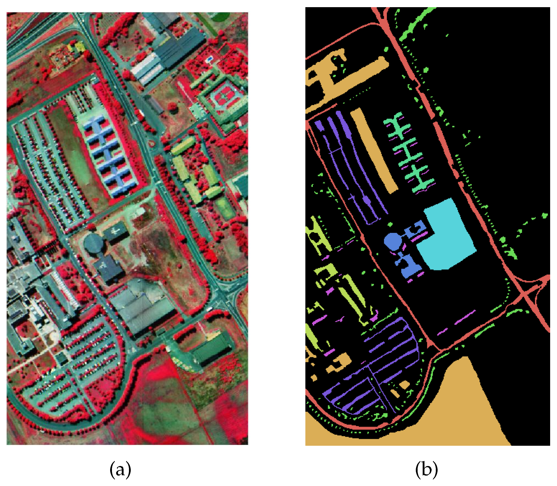
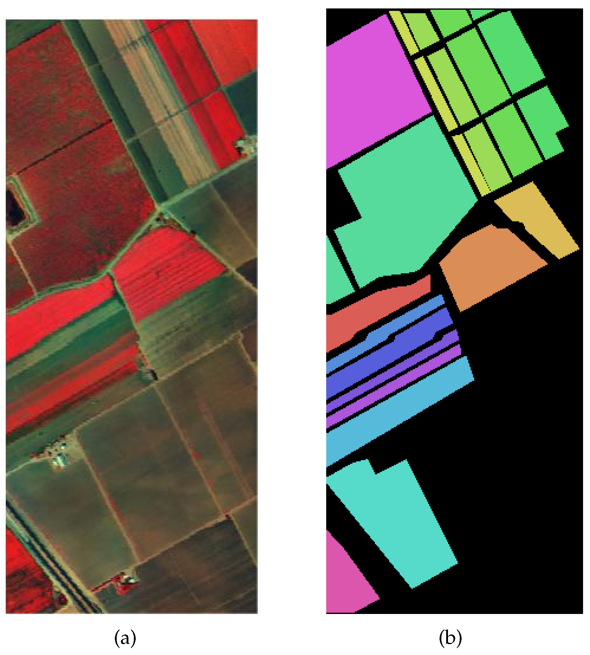
Section 4 presents the three HSI datasets, as well as the experimental setup, results, corresponding analysis. Section 5 concludes with a summary and outlook of the full paper.

2. Related Work

2.1. Deep-Learning-Based Methods for HSI Classification

Deep learning has developed quickly, more and more researchers are using deep learning methods(e.g., RNNs, CNNs, GCNs, CapsNet, LSTM) to the classification tasks of HSI [20,22,23,29,30,31,33,34]. Mei et al. [51] constructed a network based on bidirectional long short-term memory (Bi-LSTM) for HSI classification. Zhu et al. [52] proposed an end-to-end residual spectral–spatial attention network (RSSAN) for HSI classification, which consists of spectral and spatial attention modules for spectral band and spatial information adaptive selection. Song et al. [53] created a deep feature fusion network (DFFN) to solve the negative effects of excessively increasing network depth.
Due to CNN’s excellent capability of taking the local spatial context information and it’s outstanding capabilities in natural picture processing, many CNN-based HSI classification models have emerged. For example, Hang et al. [54] proposed two CNN sub-networks based on the attention mechanism for extracting the spectral and spatial features of HSI, respectively. Chakraborty et al. [55] designed a wavelet CNN that uses layers of wavelet transforms to display spectral features. Gong et al. [56] proposed a hybrid model that combines 2D-CNN and 3D-CNN in order to include more in-depth spatial and spectral features while using fewer learning samples. Hamida et al. [57] introduced a new 3-D DL method that permits the processing of both spectral and spatial information simultaneously.
However, each of these deep learning approaches has some respective drawbacks that can limit the model performance when processing HSI classification tasks. For CNN, it is good at handling two-dimensional spatial features, but since the data of HSI is stereoscopic and contains a large amount of information in the spectral dimension. It’s possible that CNN will have trouble extracting the spectral features. Moreover, although CNNs have achieved good results by relying on their local feature focus, the inability to deal with global dependencies limits their performance when processing spectral information in the form of long sequences. These shortcomings will be addressed in the transformer.

2.2. Vision Transformers for Image Classification

With the increasing use of transformers in computer vision, researchers have begun to consider images in terms of sequential data, such as ViT [42] and Swin-transformer [43] etc. Fang et al. [58] proposed MSG-Transformer, which presents a specialized token in each region as a messenger (MSG). Information can be transmitted flexibly among areas and computational cost is decreased by manipulating these MSG tokens. Guo et al. [59] proposed CMT, which combines the advantages of CNN and ViT, a new hybrid transformer-based network that captures long-range dependencies using transformers and extracts local information using CNN. Chen et al. [60] designed MobileNet and transformer in parallel, connected in the middle by a two-way bridge. This structure benefits from MobileNet for local processing and Transformer for global communication.
An increasing number of researchers are applying transformer to HSI classification tasks. Hong et al. [44] proposed a model called SpectralFormer (SF) for HSI classification, which divides neighboring bands into the same token for learning features and connects encoder blocks across layers, but the spatial information in HSI was not considered. Sun et al. [45] proposed the Spectral-Spatial Feature Tokenization Transformer (SSFTT) to capture high-level semantic information and spectral-spatial features, resulting in a large performance improvement. Ayas et al. [61] designs a spectal-swin module in front of the swin transformer, which extracts spatial and spectral features and fuses them with Conv 2-D operation and Conv 3-D operation, respectively. Mei et al. [47] proposed the Group-Aware Hierarchical Transformer (GAHT) to restrict the MSA to a local spatial-spectral range by using a new group pixel embedding module, which enables the model to have improved capability of local feature extraction. Yang et al. [46] proposed a hyperspectral image transformer (HiT) classification network that captures subtle spectral differences and conveys local spatial context information by embedding convolutional operations in the transformer structure, however it is not effective in capturing local spectral features. Transformer is increasingly used in the field of HSI classification and we believe it has great potential for the future.

3. Methodology

In this section, we will introduce the proposed spectral-swin transformer (SSWT) with spatial feature extraction enhancement, which will be described in four aspects: the overall architecture, spatial feature extraction module(SFE), spatial position encoding(SPE), and spectral swin-transformer module.

3.1. Overall Architecture

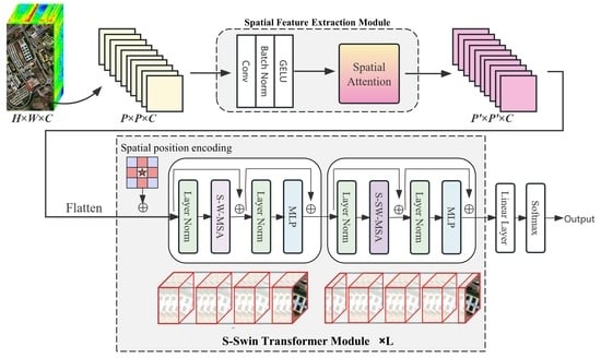
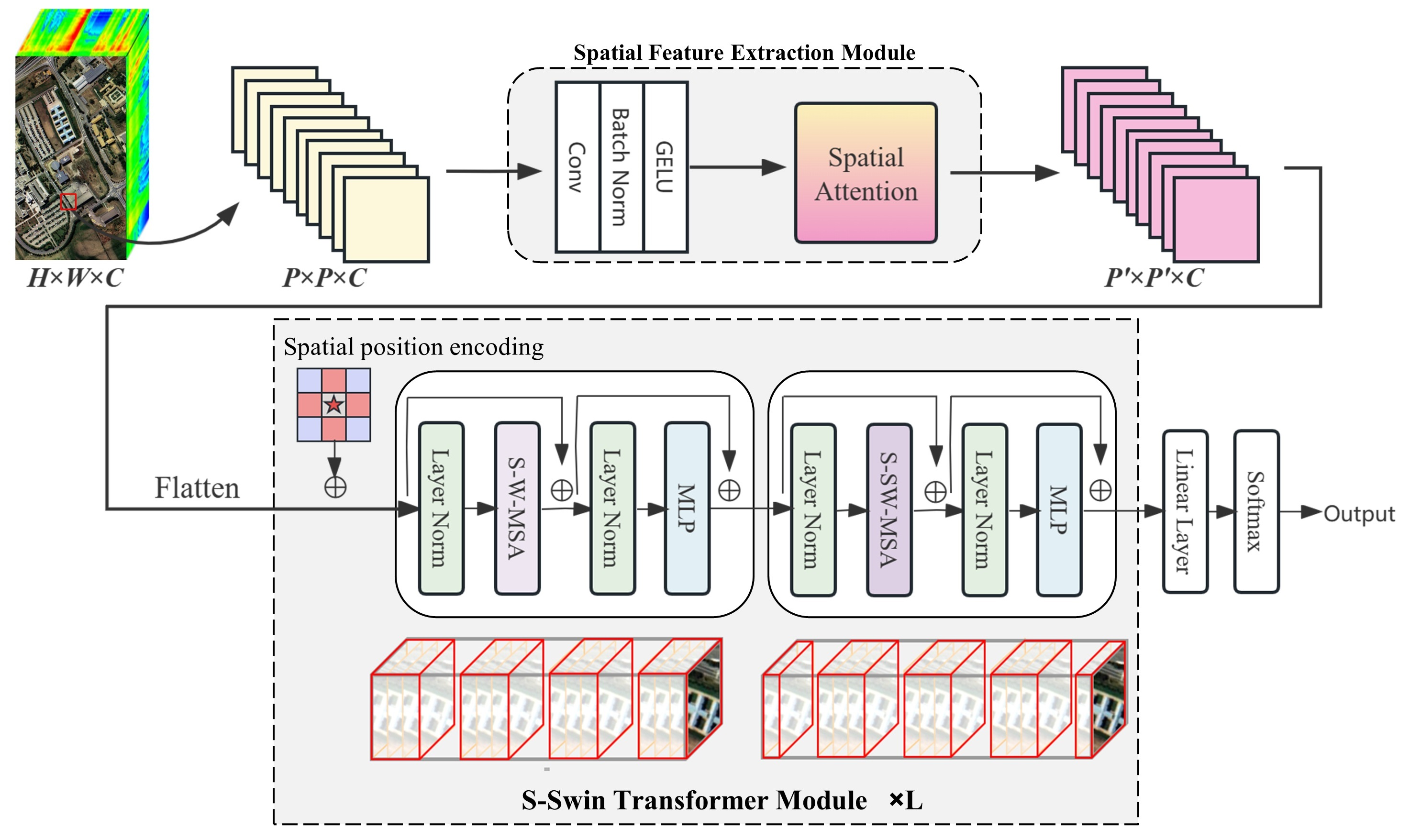
In this paper, we design a new transformer-based method SSWT for the HSI classification. SSWT consists of two major Components for solving the challenges in HSI classification, namely, spatial feature extraction module(SFE) and spectral swin(S-Swin) transformer module. An overview of the proposed SSWT for the HSI classification is shown in Figure 1. The input to the model is a patch of HSI. the data is first input to SFE to perform initial spatial feature extraction, the module consists of convolution layers and spatial attention. In Section 3.2, it is explained in further detail. The data is then flattened and entered into the s-swin transformer module. A spatial position encoding is added in front of each s-swin transformer layer to add spatial structure to the data. This part will be described in Section 3.3. The s-swin transformer module uses the spectral-swin self attention, which will be introduced in Section 3.4. The final classification results are obtained by linear layers.

3.2. Spatial Feature Extraction Module

Due to transformer’s lack of ability in handling spatial information and local features, we designed a spatial feature extraction (SFE) module to compensate. It consists of two parts, the first one consists of convolutional layers to preliminary extraction of spatial features and batch normalization to prevent overfitting. The second part is a spatial attention mechanism, which aims to enable the model to learn the important spatial locations in the data. The structure of SFE is shown in Figure 1.
For the input HSI patch cube I R H × W × C , where H × W is the spatial size and C is the number of spectral bands. Each pixel space in I consists of C spectral dimensions and forms a one-hot category vector S = s 1 , s 2 , s 3 , , s n R 1 × 1 × n , where n is the number of ground object classes.
Firstly, the spatial features of HSI are initially extracted by CNN layers, and the formula is shown as follows:
X = G E L U B N C o n v I
where C o n v ( · ) represents the convolution layer. B N ( · ) represents batch normalization. G E L U ( · ) denotes the activation function. The formula for the convolution layer is shown below:
C o n v I = | | j = 0 J ( I W j r 1 × r 2 + b j )
where I is the input, J is the number of convolution kernels, W j r 1 × r 2 is the jth convolution kernel with the size of r 1 × r 2 , and b j is the jth bias. | | denotes concatenation, and * is convolution operation.
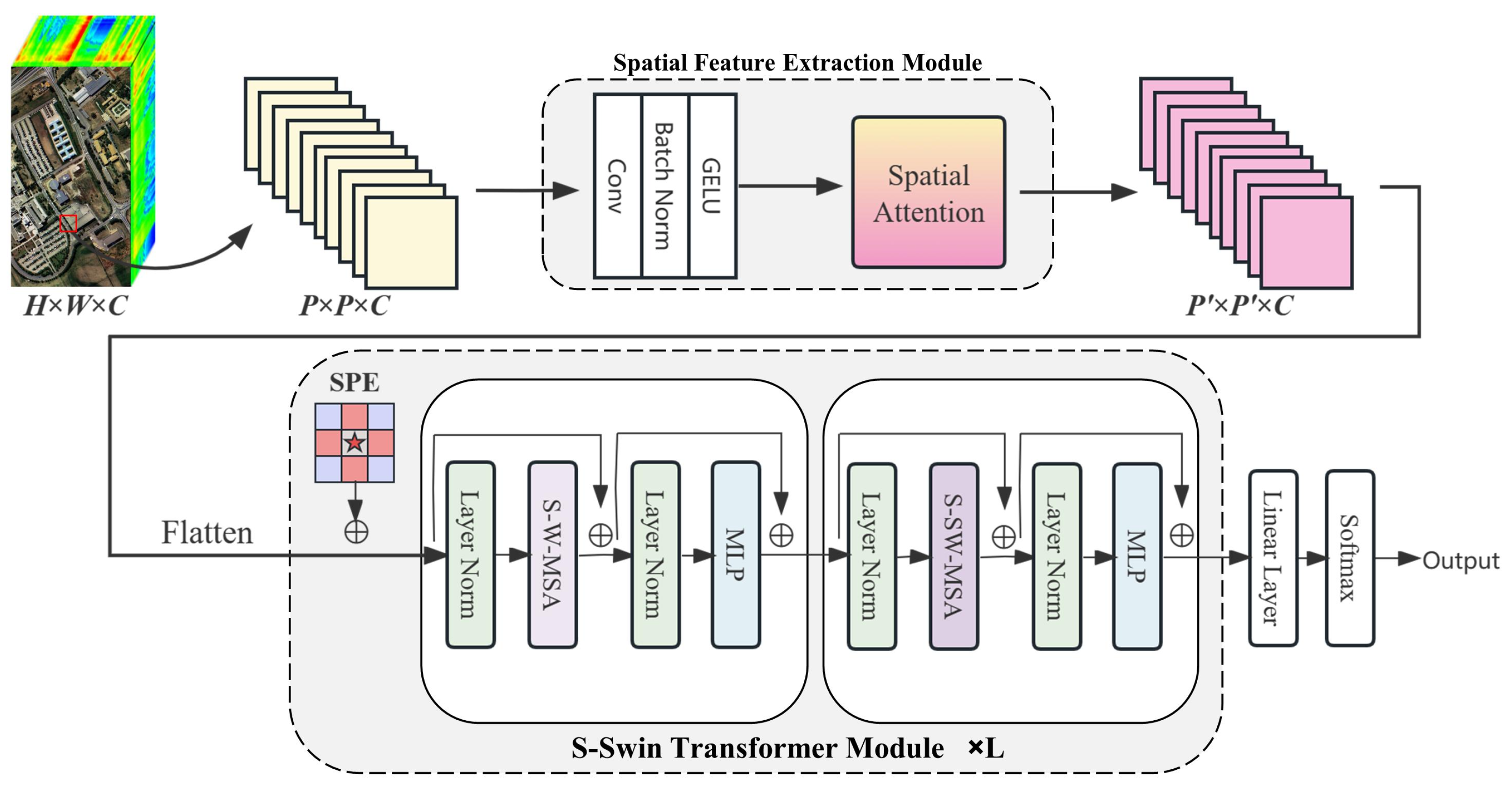
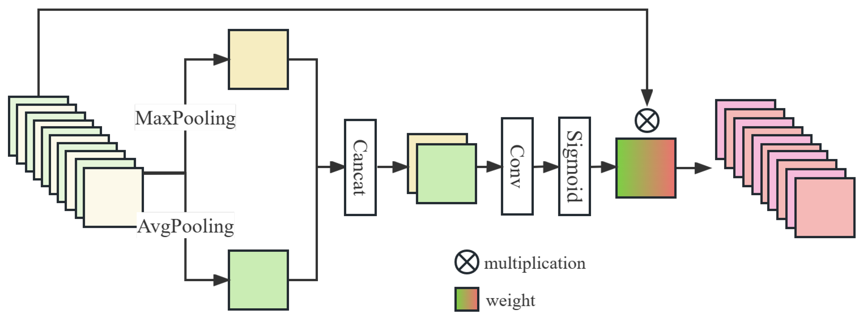
Then, the model may learn important places in the data thanks to a spatial attention mechanism (SA). The structure of SA is shown in Figure 2. For an intermediate feature map X R H × W × C ( H × W is the spatial size of X), the process of SA is shown in the following formula:
S M = M a x P o o l i n g ( X )
S A = A v g P o o l i n g ( X )
X S A = σ C o n v C o n c a t S M , S A X
MaxPooling and AvgPooling are global maximum pooling and global average pooling along the channel direction. Concat denotes concatenation in the channel direction. σ is activation function. ⊗ denotes the elementwise multiplication.

3.3. Spatial Position Encoding

The HSI of the input transformer is mapped to linear data, which can damage the spatial structure of HSI. To describe the relative spatial positions between pixels and to maintain the rotational invariance of samples, a spatial position encoding (SPE) is added before each transformer module.
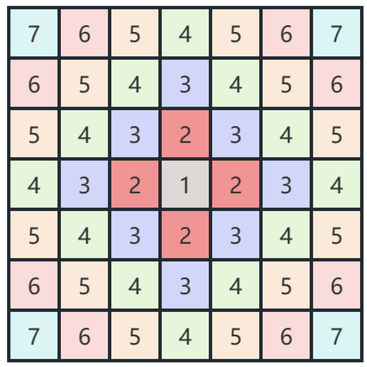
The input to HSI classification is a patch of a region, but only the label of the center pixel is the target of classification. The surrounding pixels can provide spatial information for the classification of center pixel, and their importance tends to decrease with the distance to the center. SPE is to learn such a center-important position encoding. The pixel positions of a patch is defined as follows.
p o s ( x i , y i ) = | x i x c | + | y i y c | + 1
where ( x c , y c ) denotes the coordinate of central position of the sample, that is the pixel to be classified. ( x i , y i ) denotes the coordinates of other pixels in the sample. The visualization of SPE when the spatial size of the sample is 7 × 7 can be seen in Figure 3. The pixel in the central position is unique and most important, and the other pixels are given different position encoding depending on the distance from the center.
To flexibly represent the spatial structure in HSI, the learnable position encoding are embedded in the data:
Y = X + s p e ( P )
where X is the HSI data, and P represents the position matrix (like Figure 3) constructed according to Equation (6). s p e ( · ) is a learnable array that takes the position matrix as a subscript to get the final spatial position encoding. Finally, the position encoding is added to the HSI data.

3.4. Spectral Swin-Transformer Module

The structure of the spectral swin-transformer (S-SwinT) module is shown in Figure 1. Transformer is good at processing long dependencies and lacks the ability to extract local features. Inspired by swin-transformer [
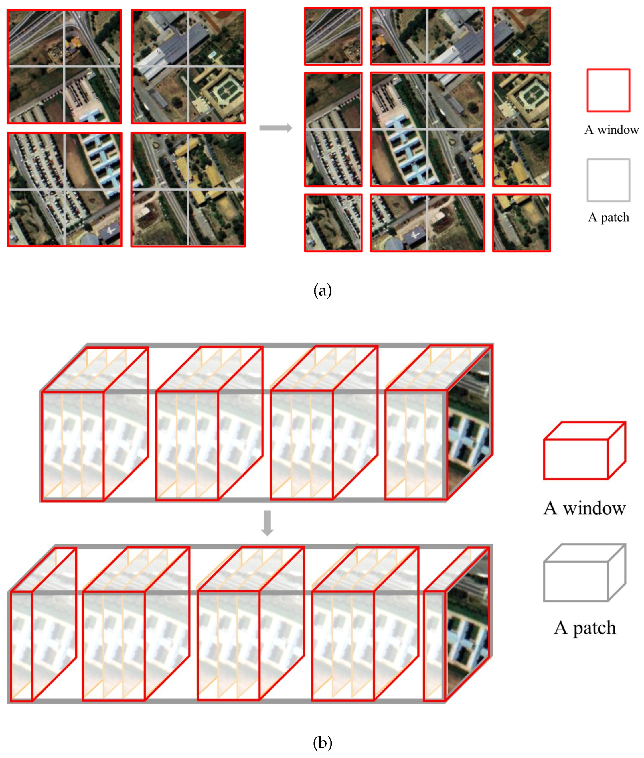
43], window-based multi-head self-attention (MSA) is used in our model. Because the input of HSI is a patch which is usually small in spatial size, it cannot divide the window in space as Swin-T does. Considering the rich data of HSI in the spectral dimension, a window of spectral shift was designed for MSA, called spectral window multi-head self-attention (S-W-MSA) and spectral shifted window multi-head self-attention (S-SW-MSA). MSA within windows can effectively improve local feature capturing, and window shifting allows information to be exchanged in the neighboring windows. MSA can be expressed by the following formula:
Z = A t t n ( Q , K , V ) = s o f t m a x Q K T d K V
ψ = C o n c a t ( Z 1 , Z 2 , , Z h ) W
Q, K, V are matrices mapped from the input matrices called queries, keys and values. d K is the dimension of K. The attention scores are calculated from Q and K. h is the head number of MSA, W denotes the output mapping matrix., and ψ represents the output of MSA.
As shown in Figure 4, the size of input is assumed to be H × W × C , where H × W is the space size and C is the number of spectral bands. Given that all windows’ size is set to C / 4 , the window is divided uniformly for the spectral dimension. The size of each window after division is [ C / 4 , C / 4 , C / 4 , C / 4 ] . Then MSA is performed in each window. Next the window is moved half a window in the spectral direction, The size of each window at this point is [ C / 8 , C / 4 , C / 4 , C / 4 , C / 8 ] . MSA is again performed in each window. Wherefore, the process of S-W-MSA with m windows is:
Y ( m ) = ψ ( y ( 1 ) ) ψ ( y ( 2 ) ) , , ψ ( y ( m ) )
where ⊕ means concat, y ( i ) is the data of the i-th window.
Compared to SwinT, the other components of the S-SwinT module remain the same except for the design of the window, such as MLP, layer normalization (LN) and residual connections. Figure 1 describes two nearby S-SwinT modules in each stage, which can be represented by the following formula.
Y ^ l = S - W - MSA ( LN ( Y l 1 ) ) + Y l 1
Y l = MLP ( LN ( Y ^ l ) ) + Y ^ l
Y ^ l + 1 = S - S W - MSA ( LN ( Y l ) ) + Y l
Y l + 1 = MLP ( LN ( Y ^ l + 1 ) ) + Y ^ l + 1
where S-W-MSA and S-SW-MSA denote the spectral window based and spectral shifted window based MSA, Y ^ l and Y l are the outputs of S-(S)W-MSA and MLP in block l.

4. Experiment

In this section, we conducted extensive experiments on three benchmark datasets to demonstrate the effectiveness of the proposed method, including Pavia University (PU), Salinas (SA) and Houston2013 (HU).

4.1. Dataset

The three datasets that utilised in the experiments are detailed here.
(1)
Pavia University:The Reflective Optics System Imaging Spectrometer (ROSIS) sensor acquired the PU dataset in 2001. It comprises 115 spectral bands with wavelengths ranging from 380 to 860 nm. Following the removal of the noise bands, there are now 103 open bands for investigation. The image measures 610 pixels in height and 340 pixels in width. The collection includes 42,776 labelled samples of 9 different land cover types.
(2)
Salinas: The Airborne Visible/Infrared Imaging Spectrometer (AVIRIS) sensor acquired the SA dataset in 1998. The 224 bands in the original image have wavelengths between 400 and 2500 nm. 204 bands are used for evaluating after the water absorption bands have been removed. The data has 512 and 217 pixels of height and width, respectively. There are 16 object classes represented in the dataset’s 54,129 marked samples.
(3)
Houston2013: The Hyperspectral Image Analysis Group and the NSF-funded Airborne Laser Mapping Center (NCALM) at the University of Houston in the US provided the Houston 2013 dataset. The 2013 IEEE GRSS Data Fusion Competition used the dataset initially for scientific research. It has 144 spectral bands with wavelengths between 0.38 and 1.05 m. This dataset contains 15 classes and measures 349 × 1905 pixels with a 2.5 m spatial resolution.
We divided the label samples in different ways for each dataset. Table 1, Table 2 and Table 3 provide specifics on the number of each class for the three dataset training, validation, and testing sets. False-color map and ground-truth map of three datasets are shown in Figure 5, Figure 6 and Figure 7.

4.2. Experimental Setting

(1)
Evaluation Indicators: To quantitatively analyse the efficacy of the suggested method and other methods for comparison, four quantitative evaluation indexes are introduced: overall accuracy (OA), average accuracy (AA), kappa coefficient ( κ ), and the classification accuracy of each class. A better classification effect is indicated by a higher value for each indicator.
(2)
Configuration: All verification experiments for the proposed technique were performed in the PyTorch environment using a desktop computer with an Intel(R) Core(TM) i7-10750H CPU, 16GB of RAM, and an NVIDIA Geforce GTX 1660Ti 6-GB GPU. The learning rate was initially set to 1 × 10 3 and the Adam optimizer was selected as the initial optimizer. The size of each training batch was set to 64. Each dataset received 500 training epochs.

4.3. Parameter Analysis

4.3.1. Influence of Patch Size

Patch size is the spatial size of the input patches, which determines the spatial information that the model can utilize when classifying HSIs. Therefore, The model’s performance is influenced by the patch size. A too large patch size will increase the computational burden of the model. In this section we compare a set of patch sizes { 3 , 5 , 7 , 9 , 11 , 13 } to explore the effect of patch size on the model. The experimental results about patch size on the three datasets are shown in Figure 8. A similar trend was observed in all three datasets, OA first increased and then stabilized with increasing patch size. Specifically, the highest value of OA is achieved when the patch size is 9 in the PU and HU datasets, and the highest value of OA is achieved when the patch size is 11 in the SA dataset.
The size of patch is positively correlated with the spatial information contained in the patch. Increasing the patch means that the model can learn more spatial information, which will be beneficial to improve OA. And when the patch increases to a certain size, the distance between the pixels in the newly region and the center pixel is too far, and the spatial information that can be provided is of little value. So the improvement of OA is not much, and the OA will tend to be stable at this time.

4.3.2. Influence of Window Number

In proposed S-SW-MSA, the number of windows is a parameter that can be set depending on the characteristics of the dataset. Moreover, the number of windows can be different for each transformer layer in order to extract multiple scales of features. We set up six sets of experiments, the model contains four transformer layers in the first four sets, and five transformer layers in the last two sets. the numbers in [ ] indicate the number of windows of S-SW-MSA in each transformer layer. The experimental results on the three datasets are shown in Table 4. According to the experimental results, the best OA for each dataset was obtained for different window number settings, and the best OA was obtained for the PU, SA and HU datasets in the 4th, 2nd and 6th group settings, respectively. We also found that increasing the number of transformer layers does not necessarily increase the performance of the model. For example, the best OA is achieved when the number of transformer layers is 4 for the PU and SA datasets and 5 for the HU dataset. Because the features of each dataset are different, the parameter settings will change accordingly.

4.4. Ablation Experiments

To sufficiently demonstrate that proposed method is effective, we conducted ablation experiments on the Pavia University dataset. With ViT as the baseline, the components of the model are added separately: S-Swin, SPE and SFE. In total, there are 5 combinations. The experimental results are shown in the Table 5. The classification overall accuracy of ViT without any improvement was 84.43 % . SPE, SFE and S-Swin are proposed improvements for the ViT backbone network, which can respectively increase classification overall accuracy of 1.69 % , 7.21 % and 7.87 % after adding into the model. The classification overall accuracy of applying the two improvements to the model together can reach 93.78 % , which is higher than baseline by 9.35 % . It is considered to be a great result for the improved pure transformer, but it’s a little lower than our final result. After the SFE was added to the model, the classification overall accuracy improved by 4.59 % , eventually reaching 98.37 .

4.5. Classification Results

The proposed model’s outcomes are compared with those of the advanced deep learning models: a LSTM based network (Bi-LSTM) [51], a 3-D CNN-based deep learning network (3D-CNN) [57], a deep feature fusion network (DFFN) [53], a RSSAN [52], and some transformer based model include a Vit, Swin-transformer (SwinT) [43], a SpectralFormer (SF) [44], a Hit [46] and a SSFTT [45].
Table 6, Table 7 and Table 8 show the OA, AA, κ and the accuracy of each category for each model’s classification on the three public datasets. Each result is the average of repeating the experiment five times. The best results are shown in bold. As the results show, proposed SSWT performs the best. On the PU dataset, SSWT is 1.02 % higher than SSFTT, 3.85 % higher than HiT, 9.01 % higher than SwinT and 1.51 % higher than RSSAN in terms of OA. Moreover, SSWT outperforms other models in terms of AA and κ . SSWT achieved the highest classification accuracy in 7 out of 9 categories. On the SA dataset, the advantage of SSWT is more prominent. SSWT is 3.22 % higher than SSFTT, 3.99 % higher than HiT, 7.10 % higher than SwinT, 2.64 % higher than RSSAN, and 3.01 % higher than DFFN in terms of OA. The same advantage was achieved for SSWT in AA and κ . SSWT achieved the highest classification accuracy in 11 out of 16 categories. Similar results can be observed in HU dataset, where SSWT achieved significant advantages in all three metrics of OA, AA and κ . SSWT achieved the highest classification accuracy in 6 out of 15 categories.
We visualized the prediction results of each model on the samples to compare the performance of the models, and the visualization results of each model on the three datasets are shown in Figure 9, Figure 10 and Figure 11 Proposed SSWT has less noise in all three datasets compared to other models, and the classification result of SSWT are closest to the ground truth. In the PU dataset, the blue area in the middle is misclassified by many models, and the SSWT result in the fewest errors. In the SA dataset, the pink area and the green area on the top left show a number of errors in the classification results of other models, and the SSWT classification results are the smoothest. A similar situation is observed in the HU dataset. The superiority of proposed model is further demonstrated.

4.6. Robustness Evaluation

In order to evaluate the robustness of the proposed model, we conducted experiments with the proposed model and other models under different numbers of training samples. Figure 12 shows the experimental results on three datasets, we selected 0.5%, 1%, 2%, 4%, and 8% of the samples in turn as training data for the PU and SA dataset, while 2%, 4%, 6%, 8% and 10% for the HU dataset. It can be observed that the proposed SSWT is performing best in every situation, especially in the case of few training samples. The robustness of proposed SSWT and its superiority in the case of small samples can be demonstrated. Taking the PU dataset as an example, most of the models achieve high accuracy at 8% of the training percent, with SSWT having a small advantage. And as the training percent decreases, SSWT has higher accuracy compared to other models. Similar results were found on the SA and HU datasets, where SSWT showed excellent performance for all training percents.

5. Conclusions

In this paper, we summarize the shortcomings of the existing ViT for HSI classification tasks. For the lack of ability to capture local contextual features, we use the self-attentive mechanism of shifted windows. The corresponding design is made for the characteristics of HSI, i.e., the spectral shifted window self-attention, which effectively improves the local feature extraction capability. For the insensitivity of ViT to spatial features and structure, we designed the spatial feature extraction module and spatial position encoding to compensate. The superiority of the proposed model has been verified by experimental results across three public HSI datasets.
In future work, we will improve the calculation of S-SW-MSA to reduce its time complexity. In addition, we will continue our research based on the transformer and try to achieve higher performance with a model of pure transformer structure.

Author Contributions

All the authors made significant contributions to the work. Y.P., J.R. and J.W. designed the research, analyzed the results, and accomplished the validation work. M.S. provided advice for the revision of the paper. All authors have read and agreed to the published version of the manuscript.

Funding

This research received no external funding.

Conflicts of Interest

The authors declare no conflict of interest.

References

  1. Gevaert, C.M.; Suomalainen, J.; Tang, J.; Kooistra, L. Generation of spectral–temporal response surfaces by combining multispectral satellite and hyperspectral UAV imagery for precision agriculture applications. IEEE J. Sel. Top. Appl. Earth Observ. Remote Sens. 2015, 8, 3140–3146. [Google Scholar] [CrossRef]
  2. Jabir, B.; Falih, N.; Rahmani, K. Accuracy and Efficiency Comparison of Object Detection Open-Source Models. Int. J. Online Biomed. Eng. 2021, 17, 165–184. [Google Scholar] [CrossRef]
  3. Lu, G.; Fei, B. Medical hyperspectral imaging: A review. J. Biomed. Opt. 2014, 19, 010901. [Google Scholar] [CrossRef]
  4. Lone, Z.A.; Pais, A.R. Object detection in hyperspectral images. Digit. Signal Process. 2022, 131, 103752. [Google Scholar] [CrossRef]
  5. Weber, C.; Aguejdad, R.; Briottet, X.; Avala, J.; Fabre, S.; Demuynck, J.; Zenou, E.; Deville, Y.; Karoui, M.S.; Benhalouche, F.Z.; et al. Hyperspectral imagery for environmental urban planning. In Proceedings of the IGARSS 2018–2018 IEEE International Geoscience and Remote Sensing Symposium, Valencia, Spain, 22–27 July 2018; IEEE: New York, NY, USA, 2018; pp. 1628–1631. [Google Scholar]
  6. Li, N.; Lü, J.S.; Altermann, W. Hyperspectral remote sensing in monitoring the vegetation heavy metal pollution. Spectrosc. Spectr. Anal. 2010, 30, 2508–2511. [Google Scholar]
  7. Saralıoğlu, E.; Görmüş, E.T.; Güngör, O. Mineral exploration with hyperspectral image fusion. In Proceedings of the 2016 24th Signal Processing and Communication Application Conference (SIU), Zonguldak, Turkey, 16–19 May 2016; IEEE: New York, NY, USA, 2016; pp. 1281–1284. [Google Scholar]
  8. Ren, J.; Wang, R.; Liu, G.; Feng, R.; Wang, Y.; Wu, W. Partitioned relief-F method for dimensionality reduction of hyperspectral images. Remote Sens. 2020, 12, 1104. [Google Scholar] [CrossRef]
  9. Ke, C. Military object detection using multiple information extracted from hyperspectral imagery. In Proceedings of the 2017 International Conference on Progress in Informatics and Computing (PIC), Nanjing, China, 15–17 December 2017; IEEE: New York, NY, USA, 2017; pp. 124–128. [Google Scholar]
  10. Cariou, C.; Chehdi, K. A new k-nearest neighbor density-based clustering method and its application to hyperspectral images. In Proceedings of the 2016 IEEE International Geoscience and Remote Sensing Symposium (IGARSS), Beijing, China, 10–15 July 2016; IEEE: New York, NY, USA, 2016; pp. 6161–6164. [Google Scholar]
  11. Ren, J.; Wang, R.; Liu, G.; Wang, Y.; Wu, W. An SVM-based nested sliding window approach for spectral–spatial classification of hyperspectral images. Remote Sens. 2020, 13, 114. [Google Scholar] [CrossRef]
  12. Yaman, O.; Yetis, H.; Karakose, M. Band Reducing Based SVM Classification Method in Hyperspectral Image Processing. In Proceedings of the 2020 Zooming Innovation in Consumer Technologies Conference (ZINC), Novi Sad, Serbia, 26–27 May 2020; IEEE: New York, NY, USA, 2020; pp. 21–25. [Google Scholar]
  13. Chen, Y.; Zhao, X.; Lin, Z. Optimizing subspace SVM ensemble for hyperspectral imagery classification. IEEE J. Sel. Top. Appl. Earth Observ. Remote Sens. 2014, 7, 1295–1305. [Google Scholar] [CrossRef]
  14. Shao, Z.; Zhang, L.; Zhou, X.; Ding, L. A novel hierarchical semisupervised SVM for classification of hyperspectral images. IEEE Geosci. Remote Sens. Lett. 2014, 11, 1609–1613. [Google Scholar] [CrossRef]
  15. Zhang, Y.; Cao, G.; Li, X.; Wang, B. Cascaded random forest for hyperspectral image classification. IEEE J. Sel. Top. Appl. Earth Observ. Remote Sens. 2018, 11, 1082–1094. [Google Scholar] [CrossRef]
  16. Belgiu, M.; Drăguţ, L. Random forest in remote sensing: A review of applications and future directions. ISPRS J. Photogramm. Remote Sens. 2016, 114, 24–31. [Google Scholar] [CrossRef]
  17. Navarro, A.; Nicastro, N.; Costa, C.; Pentangelo, A.; Cardarelli, M.; Ortenzi, L.; Pallottino, F.; Cardi, T.; Pane, C. Sorting biotic and abiotic stresses on wild rocket by leaf-image hyperspectral data mining with an artificial intelligence model. Plant Methods 2022, 18, 45. [Google Scholar] [CrossRef] [PubMed]
  18. Song, W.; Li, S.; Kang, X.; Huang, K. Hyperspectral image classification based on KNN sparse representation. In Proceedings of the 2016 IEEE International Geoscience and Remote Sensing Symposium (IGARSS), Beijing, China, 10–15 July 2016; IEEE: New York, NY, USA, 2016; pp. 2411–2414. [Google Scholar]
  19. Guo, Y.; Yin, X.; Zhao, X.; Yang, D.; Bai, Y. Hyperspectral image classification with SVM and guided filter. EURASIP J. Wirel. Commun. Netw. 2019, 2019, 56. [Google Scholar] [CrossRef]
  20. Wu, H.; Prasad, S. Convolutional recurrent neural networks for hyperspectral data classification. Remote Sens. 2017, 9, 298. [Google Scholar] [CrossRef]
  21. Luo, H. Shorten spatial-spectral RNN with parallel-GRU for hyperspectral image classification. arXiv, 2018; arXiv:1810.12563. [Google Scholar]
  22. Mou, L.; Ghamisi, P.; Zhu, X.X. Deep recurrent neural networks for hyperspectral image classification. IEEE Trans. Geosci. Remote Sens. 2017, 55, 3639–3655. [Google Scholar] [CrossRef]
  23. Lee, H.; Kwon, H. Contextual deep CNN based hyperspectral classification. In Proceedings of the 2016 IEEE International Geoscience and Remote Sensing Symposium (IGARSS), Beijing, China, 10–15 July 2016; IEEE: New York, NY, USA, 2016; pp. 3322–3325. [Google Scholar]
  24. Chen, Y.; Zhu, L.; Ghamisi, P.; Jia, X.; Li, G.; Tang, L. Hyperspectral images classification with Gabor filtering and convolutional neural network. IEEE Geosci. Remote Sens. Lett. 2017, 14, 2355–2359. [Google Scholar] [CrossRef]
  25. Zhao, X.; Tao, R.; Li, W.; Li, H.C.; Du, Q.; Liao, W.; Philips, W. Joint classification of hyperspectral and LiDAR data using hierarchical random walk and deep CNN architecture. IEEE Trans. Geosci. Remote Sens. 2020, 58, 7355–7370. [Google Scholar] [CrossRef]
  26. Chen, Y.; Jiang, H.; Li, C.; Jia, X.; Ghamisi, P. Deep feature extraction and classification of hyperspectral images based on convolutional neural networks. IEEE Trans. Geosci. Remote Sens. 2016, 54, 6232–6251. [Google Scholar] [CrossRef]
  27. He, M.; Li, B.; Chen, H. Multi-scale 3D deep convolutional neural network for hyperspectral image classification. In Proceedings of the 2017 IEEE International Conference on Image Processing (ICIP), Beijing, China, 17–20 September 2017; IEEE: New York, NY, USA, 2017; pp. 3904–3908. [Google Scholar]
  28. Makantasis, K.; Karantzalos, K.; Doulamis, A.; Doulamis, N. Deep supervised learning for hyperspectral data classification through convolutional neural networks. In Proceedings of the 2015 IEEE International Geoscience and Remote Sensing Symposium (IGARSS), Milan, Italy, 26–31 July 2015; IEEE: New York, NY, USA, 2015; pp. 4959–4962. [Google Scholar]
  29. Wan, S.; Gong, C.; Zhong, P.; Du, B.; Zhang, L.; Yang, J. Multiscale dynamic graph convolutional network for hyperspectral image classification. IEEE Trans. Geosci. Remote Sens. 2019, 58, 3162–3177. [Google Scholar] [CrossRef]
  30. Mou, L.; Lu, X.; Li, X.; Zhu, X.X. Nonlocal graph convolutional networks for hyperspectral image classification. IEEE Trans. Geosci. Remote Sens. 2020, 58, 8246–8257. [Google Scholar] [CrossRef]
  31. Paoletti, M.E.; Haut, J.M.; Fernandez-Beltran, R.; Plaza, J.; Plaza, A.; Li, J.; Pla, F. Capsule networks for hyperspectral image classification. IEEE Trans. Geosci. Remote Sens. 2018, 57, 2145–2160. [Google Scholar] [CrossRef]
  32. Yin, J.; Li, S.; Zhu, H.; Luo, X. Hyperspectral image classification using CapsNet with well-initialized shallow layers. IEEE Geosci. Remote Sens. Lett. 2019, 16, 1095–1099. [Google Scholar] [CrossRef]
  33. Zhou, F.; Hang, R.; Liu, Q.; Yuan, X. Hyperspectral image classification using spectral-spatial LSTMs. Neurocomputing 2019, 328, 39–47. [Google Scholar] [CrossRef]
  34. Gao, J.; Gao, X.; Wu, N.; Yang, H. Bi-directional LSTM with multi-scale dense attention mechanism for hyperspectral image classification. Multimed. Tools Appl. 2022, 81, 24003–24020. [Google Scholar] [CrossRef]
  35. Xu, Y.; Du, B.; Zhang, L.; Zhang, F. A band grouping based LSTM algorithm for hyperspectral image classification. In Computer Vision: Second CCF Chinese Conference, CCCV 2017, Tianjin, China, 11–14 October 2017, Proceedings, Part II; Springer: Berlin/Heidelberg, Germany, 2017; pp. 421–432. [Google Scholar]
  36. Luo, Y.; Zou, J.; Yao, C.; Zhao, X.; Li, T.; Bai, G. HSI-CNN: A novel convolution neural network for hyperspectral image. In Proceedings of the 2018 International Conference on Audio, Language and Image Processing (ICALIP), Shanghai, China, 16–17 July 2018; IEEE: New York, NY, USA, 2018; pp. 464–469. [Google Scholar]
  37. Haut, J.M.; Paoletti, M.E.; Plaza, J.; Plaza, A.; Li, J. Hyperspectral image classification using random occlusion data augmentation. IEEE Geosci. Remote Sens. Lett. 2019, 16, 1751–1755. [Google Scholar] [CrossRef]
  38. Sun, K.; Wang, A.; Sun, X.; Zhang, T. Hyperspectral image classification method based on M-3DCNN-Attention. J. Appl. Remote Sens. 2022, 16, 026507. [Google Scholar] [CrossRef]
  39. Xu, H.; Yao, W.; Cheng, L.; Li, B. Multiple spectral resolution 3D convolutional neural network for hyperspectral image classification. Remote Sens. 2021, 13, 1248. [Google Scholar] [CrossRef]
  40. Li, W.; Chen, H.; Liu, Q.; Liu, H.; Wang, Y.; Gui, G. Attention mechanism and depthwise separable convolution aided 3DCNN for hyperspectral remote sensing image classification. Remote Sens. 2022, 14, 2215. [Google Scholar] [CrossRef]
  41. Sellami, A.; Abbes, A.B.; Barra, V.; Farah, I.R. Fused 3-D spectral-spatial deep neural networks and spectral clustering for hyperspectral image classification. Pattern Recognit. Lett. 2020, 138, 594–600. [Google Scholar] [CrossRef]
  42. Dosovitskiy, A.; Beyer, L.; Kolesnikov, A.; Weissenborn, D.; Zhai, X.; Unterthiner, T.; Dehghani, M.; Minderer, M.; Heigold, G.; Gelly, S.; et al. An image is worth 16x16 words: Transformers for image recognition at scale. arXiv, 2020; arXiv:2010.11929. [Google Scholar]
  43. Liu, Z.; Lin, Y.; Cao, Y.; Hu, H.; Wei, Y.; Zhang, Z.; Lin, S.; Guo, B. Swin transformer: Hierarchical vision transformer using shifted windows. arXiv, 2013; arXiv:2103.14030. [Google Scholar]
  44. Hong, D.; Han, Z.; Yao, J.; Gao, L.; Zhang, B.; Plaza, A.; Chanussot, J. SpectralFormer: Rethinking hyperspectral image classification with transformers. IEEE Trans. Geosci. Remote Sens. 2021, 60, 1–15. [Google Scholar] [CrossRef]
  45. Sun, L.; Zhao, G.; Zheng, Y.; Wu, Z. Spectral-spatial feature tokenization transformer for hyperspectral image classification. IEEE Trans. Geosci. Remote Sens. 2022, 60, 5522214. [Google Scholar] [CrossRef]
  46. Yang, X.; Cao, W.; Lu, Y.; Zhou, Y. Hyperspectral image transformer classification networks. IEEE Trans. Geosci. Remote Sens. 2022, 60, 1–15. [Google Scholar] [CrossRef]
  47. Mei, S.; Song, C.; Ma, M.; Xu, F. Hyperspectral image classification using group-aware hierarchical transformer. IEEE Trans. Geosci. Remote Sens. 2022, 60, 5539014. [Google Scholar] [CrossRef]
  48. Xue, Z.; Xu, Q.; Zhang, M. Local transformer with spatial partition restore for hyperspectral image classification. IEEE J. Sel. Top. Appl. Earth Observ. Remote Sens. 2022, 15, 4307–4325. [Google Scholar] [CrossRef]
  49. Hu, X.; Yang, W.; Wen, H.; Liu, Y.; Peng, Y. A lightweight 1-D convolution augmented transformer with metric learning for hyperspectral image classification. Sensors 2021, 21, 1751. [Google Scholar] [CrossRef] [PubMed]
  50. Qing, Y.; Liu, W.; Feng, L.; Gao, W. Improved transformer net for hyperspectral image classification. Remote Sens. 2021, 13, 2216. [Google Scholar] [CrossRef]
  51. Mei, S.; Li, X.; Liu, X.; Cai, H.; Du, Q. Hyperspectral image classification using attention-based bidirectional long short-term memory network. IEEE Trans. Geosci. Remote Sens. 2021, 60, 1–12. [Google Scholar] [CrossRef]
  52. Zhu, M.; Jiao, L.; Liu, F.; Yang, S.; Wang, J. Residual spectral-spatial attention network for hyperspectral image classification. IEEE Trans. Geosci. Remote Sens. 2020, 59, 449–462. [Google Scholar] [CrossRef]
  53. Song, W.; Li, S.; Fang, L.; Lu, T. Hyperspectral image classification with deep feature fusion network. IEEE Trans. Geosci. Remote Sens. 2018, 56, 3173–3184. [Google Scholar] [CrossRef]
  54. Hang, R.; Li, Z.; Liu, Q.; Ghamisi, P.; Bhattacharyya, S.S. Hyperspectral image classification with attention-aided CNNs. IEEE Trans. Geosci. Remote Sens. 2020, 59, 2281–2293. [Google Scholar] [CrossRef]
  55. Chakraborty, T.; Trehan, U. Spectralnet: Exploring spatial-spectral waveletcnn for hyperspectral image classification. arXiv, 2021; arXiv:2104.00341. [Google Scholar]
  56. Gong, H.; Li, Q.; Li, C.; Dai, H.; He, Z.; Wang, W.; Li, H.; Han, F.; Tuniyazi, A.; Mu, T. Multiscale information fusion for hyperspectral image classification based on hybrid 2D-3D CNN. Remote Sens. 2021, 13, 2268. [Google Scholar] [CrossRef]
  57. Hamida, A.B.; Benoit, A.; Lambert, P.; Amar, C.B. 3-D deep learning approach for remote sensing image classification. IEEE Trans. Geosci. Remote Sens. 2018, 56, 4420–4434. [Google Scholar] [CrossRef]
  58. Fang, J.; Xie, L.; Wang, X.; Zhang, X.; Liu, W.; Tian, Q. MSG-transformer: Exchanging local spatial information by manipulating messenger tokens. arXiv, 2022; arXiv:2105.15168. [Google Scholar]
  59. Guo, J.; Han, K.; Wu, H.; Tang, Y.; Chen, X.; Wang, Y.; Xu, C. Cmt: Convolutional neural networks meet vision transformers. arXiv, 2022; arXiv:2103.14030. [Google Scholar]
  60. Chen, Y.; Dai, X.; Chen, D.; Liu, M.; Dong, X.; Yuan, L.; Liu, Z. Mobile-former: Bridging mobilenet and transformer. arXiv, 2022; arXiv:2108.05895. [Google Scholar]
  61. Ayas, S.; Tunc-Gormus, E. SpectralSWIN: A spectral-swin transformer network for hyperspectral image classification. Int. J. Remote Sens. 2022, 43, 4025–4044. [Google Scholar] [CrossRef]
Figure 1. Overall structure of the proposed SSWT model for HSI classification.
Remotesensing 15 02696 g001
Figure 2. The structure of the spatial attention in SFE.
Remotesensing 15 02696 g002
Figure 3. SPE in a sample with the spatial size is 7 × 7.
Remotesensing 15 02696 g003
Figure 4. The structure of (a) S(W)-MSA of SwinT and (b) S-(S)W-MSA of SSWT (ours).
Remotesensing 15 02696 g004
Figure 5. Visualization of PU Datasets. (a) False-color map. (b) Ground-truth map.
Remotesensing 15 02696 g005
Figure 6. Visualization of SA Datasets. (a) False-color map. (b) Ground-truth map.
Remotesensing 15 02696 g006
Figure 7. Visualization of HU Datasets. (a) False-color map. (b) Ground-truth map.
Remotesensing 15 02696 g007
Figure 8. Overall accuracy(%) with different patch sizes on the three datasets. The window numbers in transformer layers is set to [1, 2, 2, 4].
Remotesensing 15 02696 g008
Figure 9. Classification maps of different methods in PU dataset. (a) Bi-LSTM. (b) 3D-CNN. (c) RSSAN. (d) DFFN. (e) Vit. (f) SwinT. (g) SF. (h) Hit. (i) SSFTT. (j) Proposed SSWT.
Remotesensing 15 02696 g009
Figure 10. Classification maps of different methods in SA dataset. (a) Bi-LSTM. (b) 3D-CNN. (c) RSSAN. (d) DFFN. (e) Vit. (f) SwinT. (g) SF. (h) Hit. (i) SSFTT. (j) Proposed SSWT.
Remotesensing 15 02696 g010aRemotesensing 15 02696 g010b
Figure 11. Classification maps of different methods in HU dataset. (a) Bi-LSTM. (b) 3D-CNN. (c) RSSAN. (d) DFFN. (e) Vit. (f) SwinT. (g) SF. (h) Hit. (i) SSFTT. (j) Proposed SSWT.
Remotesensing 15 02696 g011
Figure 12. Classification results in different training percent of samples on the three datasets. (a) PU. (b) SA. (c) HU.
Remotesensing 15 02696 g012
Table 1. Number of training, validation and testing samples for the PU dataset.
Remotesensing 15 02696 i001
Table 2. Number of training, validation and testing samples for the SA dataset.
Remotesensing 15 02696 i002
Table 3. Number of training, validation and testing samples for the HU dataset.
Remotesensing 15 02696 i003
Table 4. Overall accuracies (%) of proposed model with different number of windows in transformer layers on SA, PU and HU datasets. The patch size is set to 9.
Windows SizePUSAHU
[ 1 , 1 , 2 , 2 ] 97.0597.5693.24
[ 1 , 2 , 2 , 4 ] 97.8697.8093.35
[ 2 , 2 , 4 , 4 ] 98.3396.9393.31
[ 2 , 2 , 4 , 8 ] 98.3797.7093.58
[ 1 , 1 , 2 , 4 , 8 ] 98.2096.2593.38
[ 2 , 2 , 4 , 4 , 8 ] 98.2596.3193.69
Table 5. Ablation experiments in PU.
MethodModule (%)Metric (%)
S-SwinSPESFEOA(%)AA(%) κ × 100 (%)
ViT(Baseline)84.4378.0678.95
ViT86.1280.1881.31
ViT91.6490.4388.97
SSWT(Ours)92.3089.5889.75
SSWT(Ours)93.7891.1791.74
SSWT(Ours)98.3797.2597.84
Table 6. Classification results of the PU dataset.
ClassBi-LSTM3D-CNNRSSANDFFNVitSwinTSFHitSSFTTSSWT
191.67 ± 0.8395.16 ± 1.5697.12 ± 0.5796.66 ± 0.8187.96 ± 1.8093.05 ± 5.3289.41 ± 2.2393.72 ± 1.4497.31 ± 1.1298.06 ± 0.24
296.96 ± 1.6098.31 ± 0.9699.46 ± 0.1199.05 ± 0.5196.56 ± 3.0096.98 ± 1.4397.22 ± 0.7698.66 ± 0.4899.37 ± 0.2699.91 ± 0.08
370.65 ± 9.7336.91 ± 6.1885.74 ± 5.0570.37 ± 12.5653.18 ± 19.3529.49 ± 23.0877.28 ± 3.1980.42 ± 7.5687.25 ± 5.4394.59 ± 2.40
492.88 ± 2.7895.52 ± 1.5896.92 ± 1.3294.22 ± 3.1689.76 ± 2.2592.09 ± 1.4190.80 ± 1.9294.74 ± 1.8497.59 ± 1.1597.70 ± 1.05
599.10 ± 0.6099.83 ± 0.3499.86 ± 0.1799.97 ± 0.06100.00 ± 0.0099.16 ± 0.59100.00 ± 0.0099.95 ± 0.0499.95 ± 0.0699.85 ± 0.27
667.03 ± 14.7649.91 ± 12.1797.00 ± 1.0995.07 ± 3.0351.97 ± 7.0588.47 ± 5.0382.13 ± 6.0295.54 ± 2.0597.00 ± 1.6098.37 ± 1.63
782.67 ± 3.3146.74 ± 14.0584.15 ± 5.6674.68 ± 7.8647.59 ± 8.3645.18 ± 31.4752.80 ± 6.2375.17 ± 8.0591.43 ± 3.7091.95 ± 5.61
883.17 ± 3.2589.73 ± 3.0092.49 ± 1.5187.38 ± 4.3478.79 ± 8.8892.76 ± 1.6581.81 ± 4.4485.83 ± 4.1993.81 ± 1.5195.35 ± 5.61
998.94 ± 0.5198.66 ± 0.6298.37 ± 0.9699.57 ± 0.2296.71 ± 1.0076.85 ± 12.0996.32 ± 1.3897.16 ± 1.2999.72 ± 0.2099.48 ± 0.88
OA(%)89.52 ± 1.9186.63 ± 1.4396.86 ± 0.3694.74 ± 1.4084.43 ± 1.5689.36 ± 3.1490.16 ± 0.8994.52 ± 1.0397.35 ± 0.4598.37 ± 0.24
AA(%)87.01 ± 1.9778.97 ± 2.0594.57 ± 0.8490.77 ± 2.4678.06 ± 2.5679.34 ± 7.4685.31 ± 1.2091.24 ± 1.9495.94 ± 0.7397.25 ± 0.64
κ × 100 85.94 ± 2.6381.79 ± 2.0495.84 ± 0.4893.00 ± 1.8778.95 ± 2.0385.82 ± 4.2386.87 ± 1.2192.74 ± 1.3796.49 ± 0.6097.84 ± 0.32
Table 7. Classification results of the SA dataset.
ClassBi-LSTM3D-CNNRSSANDFFNVitSwinTSFHitSSFTTSSWT
179.24 ± 39.6397.09 ± 1.4699.58 ± 0.4897.12 ± 0.8990.19 ± 2.5172.30 ± 1.8795.05 ± 1.4998.69 ± 2.0599.44 ± 0.9099.79 ± 0.43
298.94 ± 0.5599.90 ± 0.0899.36 ± 0.8799.58 ± 0.1498.05 ± 1.1797.24 ± 1.9299.32 ± 0.1899.32 ± 0.3599.80 ± 0.3499.80 ± 0.17
385.20 ± 12.2388.23 ± 4.3597.01 ± 1.6395.01 ± 3.5487.52 ± 1.8389.31 ± 2.9692.89 ± 1.2995.51 ± 2.2998.41 ± 1.0498.48 ± 1.54
497.79 ± 1.2198.22 ± 1.1098.56 ± 0.7096.67 ± 1.3994.11 ± 1.4396.12 ± 1.5094.05 ± 2.0298.82 ± 0.5199.59 ± 0.5698.53 ± 1.23
596.40 ± 1.2293.41 ± 2.4196.06 ± 1.3796.87 ± 1.0482.59 ± 2.9397.68 ± 0.7693.24 ± 1.8396.03 ± 2.1798.28 ± 0.7798.74 ± 0.80
699.46 ± 0.3799.79 ± 0.3299.36 ± 1.0099.84 ± 0.3099.44 ± 0.6498.89 ± 1.2999.68 ± 0.3699.99 ± 0.0299.98 ± 0.0299.96 ± 0.06
798.84 ± 0.3699.47 ± 0.2399.28 ± 0.4099.62 ± 0.2898.05 ± 0.7197.79 ± 0.9298.81 ± 0.4798.88 ± 0.6299.44 ± 0.4699.72 ± 0.42
883.66 ± 3.8582.53 ± 2.3690.93 ± 2.8789.16 ± 1.7482.79 ± 1.9387.64 ± 1.3885.03 ± 2.4688.55 ± 1.7390.08 ± 4.0695.87 ± 1.47
997.84 ± 1.3498.51 ± 1.1199.66 ± 0.2698.88 ± 0.8096.38 ± 0.5799.16 ± 0.6398.05 ± 0.6499.62 ± 0.3799.53 ± 0.2499.92 ± 0.06
1081.10 ± 8.6289.40 ± 2.5095.58 ± 2.4895.39 ± 1.0175.44 ± 3.8189.52 ± 3.7491.23 ± 2.2893.74 ± 2.3895.73 ± 2.5897.07 ± 1.88
1183.59 ± 6.8373.95 ± 4.6593.37 ± 5.7592.56 ± 5.8170.47 ± 15.2983.99 ± 14.4989.86 ± 4.7491.16 ± 6.1994.66 ± 4.6695.64 ± 4.52
1298.84 ± 0.6199.21 ± 0.5699.36 ± 0.7999.97 ± 0.0398.67 ± 1.3195.76 ± 0.7598.45 ± 1.4699.30 ± 0.6499.80 ± 0.2899.78 ± 0.45
1394.78 ± 2.7299.66 ± 0.0798.92 ± 0.9999.98 ± 0.0496.28 ± 2.0594.92 ± 6.3198.61 ± 0.9298.99 ± 1.1299.06 ± 1.6699.87 ± 0.18
1490.20 ± 2.5197.24 ± 1.0596.63 ± 0.5798.52 ± 0.7696.51 ± 1.3894.47 ± 1.0495.03 ± 2.3297.16 ± 0.7795.61 ± 2.8899.23 ± 0.55
1578.87 ± 9.6673.91 ± 2.4786.60 ± 3.2787.97 ± 2.8172.03 ± 5.5086.75 ± 6.2679.87 ± 3.0081.79 ± 3.3481.36 ± 6.0994.10 ± 2.05
1690.27 ± 9.6292.36 ± 1.4696.67 ± 1.2795.16 ± 2.3291.57 ± 0.7592.77 ± 3.3095.35 ± 0.9996.79 ± 1.6797.20 ± 1.0298.40 ± 1.08
OA(%)89.66 ± 3.0390.22 ± 0.7095.16 ± 0.3594.79 ± 0.8087.58 ± 0.3790.70 ± 2.3891.81 ± 0.7393.81 ± 0.5694.58 ± 0.4197.80 ± 0.25
AA(%)90.94 ± 3.3192.68 ± 0.7196.68 ± 0.4996.39 ± 0.5789.38 ± 0.5190.02 ± 3.9994.03 ± 0.4895.90 ± 0.2496.75 ± 0.2698.43 ± 0.35
κ × 100 88.49 ± 3.3989.11 ± 0.7794.61 ± 0.3994.20 ± 0.8986.17 ± 0.4189.63 ± 2.6790.89 ± 0.8193.10 ± 0.6293.97 ± 0.4697.55 ± 0.28
Table 8. Classification results of the HU dataset.
ClassBi-LSTM3D-CNNRSSANDFFNVitSwinTSFHitSSFTTSSWT
184.09 ± 4.7789.90 ± 6.6295.05 ± 2.7794.71 ± 5.7990.72 ± 6.2194.56 ± 2.5595.05 ± 5.1093.37 ± 4.5493.96 ± 4.3295.13 ± 4.45
290.60 ± 7.7181.28 ± 6.0898.05 ± 1.1997.75 ± 1.0683.93 ± 9.7093.93 ± 5.8393.53 ± 3.7797.78 ± 0.8798.71 ± 1.1198.77 ± 1.18
375.14 ± 17.7091.81 ± 4.0498.67 ± 0.8199.49 ± 0.7488.01 ± 8.5096.68 ± 1.9897.19 ± 2.0198.64 ± 0.9199.52 ± 0.8999.46 ± 0.67
490.83 ± 3.7091.91 ± 0.3594.06 ± 1.9191.34 ± 0.7485.63 ± 3.3594.42 ± 2.7789.54 ± 1.7995.35 ± 1.9996.65 ± 2.5595.75 ± 1.55
592.86 ± 2.9395.97 ± 1.8398.29 ± 0.7798.44 ± 0.7495.86 ± 1.7597.99 ± 0.7496.97 ± 0.9298.69 ± 0.9899.54 ± 0.4999.93 ± 0.08
652.43 ± 31.3272.69 ± 2.1580.58 ± 6.7086.15 ± 6.726.93 ± 7.3471.20 ± 14.2063.88 ± 5.2081.49 ± 2.8590.42 ± 6.3292.62 ± 5.67
772.93 ± 9.3284.15 ± 2.5087.09 ± 3.5684.60 ± 3.9864.32 ± 11.1171.84 ± 14.6274.67 ± 4.0681.16 ± 5.2986.22 ± 5.4388.70 ± 4.61
855.74 ± 5.2455.87 ± 6.1478.88 ± 3.6479.10 ± 3.8266.84 ± 6.8073.69 ± 9.9076.31 ± 2.7678.85 ± 2.0382.79 ± 2.8185.08 ± 3.38
973.05 ± 5.7581.90 ± 2.1381.77 ± 4.7284.24 ± 4.7566.24 ± 5.5673.28 ± 2.7572.94 ± 6.6083.62 ± 5.8189.96 ± 4.2487.47 ± 3.31
1039.43 ± 20.4948.10 ± 12.5189.76 ± 0.5290.22 ± 5.1263.29 ± 5.9278.56 ± 2.6681.13 ± 5.7986.14 ± 5.1193.60 ± 1.2996.05 ± 3.71
1166.55 ± 10.8560.66 ± 2.6382.85 ± 4.3582.46 ± 3.6458.67 ± 3.0876.21 ± 0.3768.80 ± 6.5479.52 ± 4.9486.36 ± 2.8287.55 ± 5.08
1267.21 ± 9.9058.29 ± 10.8692.13 ± 2.7393.10 ± 2.0061.69 ± 6.3287.50 ± 3.5285.02 ± 4.1890.96 ± 3.2288.95 ± 5.9097.83 ± 1.12
1319.96 ± 14.6559.10 ± 10.8271.21 ± 8.1792.47 ± 1.5740.09 ± 16.8671.60 ± 2.7050.85 ± 9.6779.28 ± 2.8692.33 ± 2.8190.76 ± 3.15
1489.93 ± 8.8293.12 ± 3.7692.38 ± 3.9194.74 ± 2.6577.49 ± 4.4789.03 ± 7.1278.28 ± 3.0293.96 ± 2.8896.46 ± 2.2494.55 ± 3.68
1590.91 ± 8.7899.39 ± 0.7795.82 ± 2.6298.88 ± 0.8891.48 ± 3.1296.65 ± 1.7595.15 ± 2.8498.47 ± 1.0398.66 ± 1.1398.63 ± 1.56
OA(%)72.60 ± 3.0376.73 ± 1.6989.76 ± 0.3990.62 ± 0.7972.80 ± 1.5484.78 ± 2.3982.97 ± 0.9989.16 ± 1.0392.47 ± 0.9793.69 ± 1.07
AA(%)70.78 ± 4.4977.61 ± 1.8089.11 ± 0.6191.18 ± 0.8669.41 ± 0.7384.48 MSA 1.6781.29 ± 1.1689.15 ± 0.8892.94 ± 1.0193.89 ± 1.07
κ × 100 70.34 ± 3.2974.84 ± 1.8388.93 ± 0.4289.86 ± 0.8570.58 ± 1.6483.55 MSA 2.5881.58 ± 1.0788.28 ± 1.1191.86 ± 1.0593.18 ± 1.16
Disclaimer/Publisher’s Note: The statements, opinions and data contained in all publications are solely those of the individual author(s) and contributor(s) and not of MDPI and/or the editor(s). MDPI and/or the editor(s) disclaim responsibility for any injury to people or property resulting from any ideas, methods, instructions or products referred to in the content.

