Article

YOLO for Penguin Detection and Counting Based on Remote Sensing Images

1
College of Information Science and Electronic Engineering, Zhejiang University, Hangzhou 310013, China
2
Ocean College, Zhejiang University, Zhoushan 316021, China
3
Antarctic Greatwall Ecology National Observation and Research Station, Polar Research Institute of China, Shanghai 200136, China
*
Author to whom correspondence should be addressed.
Remote Sens. 2023, 15(10), 2598; https://doi.org/10.3390/rs15102598
Submission received: 7 April 2023 / Revised: 10 May 2023 / Accepted: 12 May 2023 / Published: 16 May 2023

Abstract

:
As the largest species of birds in Antarctica, penguins are called “biological indicators”. Changes in the environment will cause population fluctuations. Therefore, developing a penguin census regularly will not only help carry out conservation activities but also provides a basis for studying climate change. Traditionally, scholars often use indirect methods, e.g., identifying penguin guano and establishing regression relationships to estimate the size of penguin colonies. In this paper, we explore the feasibility of automatic object detection algorithms based on aerial images, which locate each penguin directly. We build a dataset consisting of images taken at 400 m altitude over the island populated by Adelie penguins, which are cropped with a resolution of 640 × 640. To address the challenges of detecting minuscule penguins (often 10 pixels extent) amidst complex backgrounds in our dataset, we propose a new object detection network, named YoloPd (Yolo for penguin detection). Specifically, a multiple frequency features fusion module and a Bottleneck aggregation layer are proposed to strengthen feature representations for smaller penguins. Furthermore, the Transformer aggregation layer and efficient attention module are designed to capture global features with the aim of filtering out background interference. With respect to the latency/accuracy trade-off, YoloPd surpasses the classical detector Faster R-CNN by 8.5% in mean precision (mAP). It also beats the latest detector Yolov7 by 2.3% in F1 score with fewer parameters. Under YoloPd, the average counting accuracy reaches 94.6%, which is quite promising. The results demonstrate the potential of automatic detectors and provide a new direction for penguin counting.

Graphical Abstract

1. Introduction

In the past 30 years, the Antarctic and Southern Ocean Marine ecosystems have been undergoing great changes [1]. Turel [2] statistically analyzed the meteorological data of 17 stations in Antarctica and disclosed that the Amundsen Sea’s low pressure significantly warmed the Antarctic Peninsula by changing the radial component of the wind, which certainly had important implications for the Antarctic ecosystem.
As the largest species of birds in Antarctica, penguins are labeled as “biological indicators” [3]. Environmental changes influence their survival and reproduction. Therefore, it is of great significance to monitor the changes in the penguin population, which can provide bases for discovering an environmental urgency [4]. On the other hand, the Commission for the Conservation of Antarctic Marine Living Resources (CCAMLR) revised the Ecosystem Monitoring Program [5], including four species of penguins (Adelie penguin, chinstrap penguin, gentoo penguin and macaroni penguin) as dependent species that rely on harvested species for survival. By studying various life parameters, such as population size, breeding success and foraging behavior, changes in the abundance of harvested species (e.g., krill) can be detected. Thus, monitoring penguin populations provides valuable information to implement sustainable commercial fishing plans. In this paper, based on the characteristics of our dataset, we concentrate on investigating changes in the Adelie penguin’s population size from the perspective of statistical penguin counting.
Currently, research data on penguins mainly include satellite remote sensing, aviation and field investigation [6]. Due to the limitations of climate and time costs, field investigation is mostly abandoned. Remote sensing images have emerged as the primary means for investigation of penguin distribution evolution. However, the ground resolution is low even in high-resolution satellite remote sensing images. Often penguins cannot be directly observed from images and an indirect regression relationship was established to count penguins. A variety of remote sensing data, such as Landsat and Quickiro-2, have been used to determine the changes in the penguin population [7,8]. Medium-resolution Landsat-7 is commonly used to map Adelie penguin colonies on a continental scale and high-resolution satellite images taken by Worldview can be used for detection of single or multiple penguin species. Witharana et al. used seven fusion algorithms to further enhance the resolution of high-resolution images [9].
In the 1980s, M.R. et al. [10] proposed to identify the guano region through satellite remote sensing images and then established a linear regression relationship between the area of guano and the size of Adelie penguin populations. Since then, scholars adopt supervised classification and object-oriented methods to extract fecal areas. Ref. [11] proposed a semantic segmentation network to improve the accuracy of feces extraction. However, the cost of acquiring satellite images is high; aerial images can be used as its substitute, whose ground resolution is higher. An unmanned aerial vehicle (UAV) system was used in [12] to observe the active nests of Southern Giant Petrel (SGP) on the Antarctic Specially Managed Area no. 1, Admiralty Bay, King George Island. In contrast, the penguin population has a larger community and dense distribution, which requires a large (if not prohibitive) amount of manpower and time to obtain sufficiently accurate data statistics in Antarctica. To overcome it, Ref. [13] suggested a method called Population Counting with Overhead Robotic Networks (POPCORN) to optimize the flying trajectory of UAV. Eventually, they used five drones to complete the sampling of 300,000 penguin burrows (~ 2 k m 2 ) on Ross Island, Antarctica within 3 h. In addition, Clarel developed a semi-automated workflow for counting individuals by fusing multi-spectral and thermal images by UAV [14], proving that the method was effective in most cases but may produce large errors in large population sizes. Based on those fused aerial images, an object-oriented method was developed to distinguish penguins from rock shadows [15], achieving an average accuracy of 91%.
The above indirect counting method relies heavily on manual design and prior knowledge. When the environment changes, the model may deviate significantly from reality. In 2012, convolution (Conv) was first introduced into machine learning [16], significantly improving accuracy and speed over traditional algorithms in image classification. Since then, the convolutional neural network (CNN) has played a dominant role in computer vision research and applications. By leveraging deep learning-based image processing methods to accurately locate each penguin, we can not only count the numbers but also achieve better explanatory power and robustness.
Object detection is meant to find all objects of interest from images, extracting the image features through, for example, CNN and returning the categories in detection boxes. Recently, multiple high-performance algorithms such as region convolutional neural network (R-CNN) series [17,18,19], Yolo series [20,21,22,23,24,25,26] and Vision Transformer (ViT) [27,28] have exceeded the accuracy of human vision in detecting small targets.
R-CNN [17] was the first deep learning detector that used the selective search method to generate around 2000 proposals where objects might exist. Linear regression was then used to refine the target position after a Support Vector Machine (SVM). While R-CNN outperformed other detectors, it had poor computational efficiency. To speed up training, Fast R-CNN [18] adopted the spatial pyramid pool layer to extract features from the entire image and Faster R-CNN [19] proposed using a region proposal network to replace the selective search method, significantly improving speed. Despite satisfying visual detection needs, the R-CNN series’ speed has always been a concern.
In contrast, Yolo [20] was another method that used a single CNN network to regress detection boxes and categories by fusing two steps in R-CNN, resulting in higher speed with the same network size. However, the number of detections was limited. Yolov2 [21] divided feature maps into grids, with each grid producing nine preset bounding boxes (Anchors) that were friendly for dense detection. It predicted the offset of Anchors to acquire more detections. In 2018, Yolov3 [19] fused multi-scale features to predict features with three different sizes, surpassing Faster R-CNN in both speed and accuracy. Moreover, Yolov4 [23], Yolov5 [24], Yolov6 [25], and Yolov7 [26] integrated more tricks to achieve better speed and accuracy. With its excellent balance between speed and accuracy, the Yolo series has been widely applied in target detection, especially for small objects. For example, Refs. [29,30] improved the detection performance of road cracks and potholes on the basis of Yolov3 by optimizing multi-scale fusion modules, k-means, and loss functions. The former increased F1 by 8.8%, while the latter further increased F1 by 15.4% by combining data augmentation techniques. Yolov4 was first introduced in oil derrick detection in [31], achieving excellent performance. Refs. [32,33,34] utilized Yolov5 to perform pedestrian detection in aerial images, surpassing other SOTA (state of the art) algorithms. Ref. [35] improved the Backbone of Yolov7 by space-to-depth convolution to reduce feature loss for small targets during down-sampling, further enhancing the accuracy of pedestrian detection. To increase the amount of information, an adaptive illumination-driven input-level fusion module was proposed in [36] to fuse infrared and RGB images. Similarly, Ref. [37] added an attention module during feature fusion to focus more on the scattered information, improving the accuracy of ship detection in synthetic aperture radar images.
Remote sensing image object detection has the same theoretical basis as general detectors. However, there are also differences in the detailed implementation according to the objects’ characteristics. The penguin detection case has the following difficulties:
  • The scale variation of objects is large;
  • The target distribution is dense and the pixel size can be very small (width < 10 pixels);
  • High-resolution imaging of large areas (hundreds of millions of pixels) leads to huge hardware overhead.
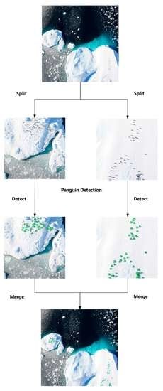
In order to solve problems similar to those above, YOLT [38] divided the remote sensing image (millions of pixels) into blocks size of 416 × 416 by a sliding window with 15% pixels overlap. The improved Yolov2 network was trained to detect cars with five pixels in size with a detection accuracy (e.g., F1 score) of 85%. An unsupervised two-stage detection method [39] enhanced the accuracy of small ships (a few tens of pixels) by scanning for potential target areas of the ship first. This was followed by a detector to execute localization and classification, significantly reducing data annotation costs. In addition, deformable convolutions [40] and parallel Region Proposal networks (RPN) [41] are incorporated into the Feature Pyramid Networks (FPN) [42] to integrate multi-scale features in order to counteract the scale variations in remote sensing imagery, remarkably boosting the detection performance of vehicles which are densely dispersed.
Furthermore, several studies are investigating the use of deep learning applications for wildlife monitoring with the aid of aerial images. Duporge et al. [43] used Faster R-CNN to identify elephants in satellite images, exceeding human vision with an F1 of 0.75. Ref. [44] compared the accuracies of three detection algorithms in recognizing six species (elephant, buffalo, African water antelope, corner wildebeest, warthog, and African oryx). Ref. [45] detects large marine animals such as dolphins that are easily confused with sunlight by abnormal thermal images. Moreover, small and medium-sized animals such as rabbits, kangaroos, wild boars [46], domestic cattle [47] and birds [48] can be rapidly detected with an accuracy rate of over 90% from in UAV-required images.
Note that, in contrast to the cars, ships, rabbits or other animals in remote sensing images, penguins appear to be smaller and the harsh conditions in Antarctica result in a higher cost for obtaining images. These challenges make it difficult to develop direct methods for penguin recognition in images. Fortunately, with the support of the Polar Research Institute of China, we obtain high-resolution aerial remote-sensing images of Adelie penguins in Antarctica. When viewed from above, penguins appear as black dots that contrast with the white snow and rocks background, making them easily detectable in images. Motivated by the deep learning method, we establish a penguin detection dataset and propose a new network for counting Adelie penguins based on their characteristics. Our overall contributions call be summarized as follows:
  • We explore the flexibility of directly counting penguins from remote-sensing images. Based on deep learning method, a penguin detection dataset is established, which includes 58 high-resolution images of 9504 × 6336 captured over the Antarctic island.
  • To address the challenges of detecting tiny penguins from significant background interference, we propose an automatic detection network, named YoloPd, for counting penguins directly and investigate its performances in the dataset we established.
  • We design the multiple frequency features fusion module (named MAConv) and Bottleneck efficient aggregation layer (BELAN) to increase the informative content of small penguins, providing deeper semantic features. Additionally, we incorporated a lightweight Swin-Transformer (LSViT) and attention mechanism into BELAN (named TBELAN and AELAN, respectively) to extract low-frequency information that can effectively help the network filter out complex background interference.
  • We reconstruct the penguin detection datasets using Gaussian kernels with varying degrees of blur and validate the feasibility of YoloPd within them. Furthermore, we also verify the robustness of YoloPd on the DOTA dataset [49].

2. Materials and Methods

2.1. Penguin Dataset

2.1.1. Data Preparation

The Polar Research Institute of China is the only scientific research and support center in China dedicated to polar exploration. We have the privilege of collaborating with them and obtained national permission from the relevant authorities to carry out the counting penguin project from remote-sensing imagery. Based on the images captured over the island ( 53.7742 °   S , 65.844 °   E ) on 1 January 2019 during China’s Antarctic Expedition, we conduct the deep learning exploration in penguin detection. The image acquisition method is described as follows:
  • A high-definition camera (SONY-ILCE-7RM4) was equipped on a helicopter to complete the remote-sensing task in a clear day with sufficient sunlight.
  • The helicopter was positioned 400 m over the island and flew in an elliptical trajectory around the entire island while maintaining a stable horizontal position.
  • During the flight, the camera was set to take an image per second, with a ground resolution exceeding 5 cm/pixel, until the entire island was covered.
Please note that in Ref. [12], keeping the aircraft at a height of 130 m above ground level will not cause any change in bird behavior. Throughout the data acquisition process, we followed the requirements of PRAS Guidelines [50] by maintaining the altitude of the aircraft at 400 m above the island to ensure the survival of the penguins was not impacted. The filming took place during the summer when the penguin breeding season had already ended. The investigation did not affect their breeding.
In addition, the entire island is dominated by Adelie penguins and for other bird species, we only found a few skuas flying in the air. Overall, this is unlikely to introduce false positives in the detection of penguins.
We select 58 high-quality images with a resolution of 9504 × 6336 covering different parts of the island. Figure 1 shows some examples. Since the adjacent images overlapped by a small part, we divide the images containing overlapping areas into different sets, getting 40 training images and 18 validation images. Both training and validation sets contain sparse and densely distributed scenes. Among them, a single image contains a minimum of five penguins and a maximum of 2580 penguins. The distribution of penguins on the island is extremely uneven, which brings great challenges to our experiment.

2.1.2. Data Processing

As obtained high-definition images through precise equipment, we directly processed the original images into formats that can be used for deep learning. Firstly, we use the software LabelImg [51] to annotate all the images, identifying each penguin and marking it with a rectangle box. Among them, we acquire a total of 32,567 annotated instances. Similar to YOLT, 58 images are cut into sub-images with the size of 640 × 640. All adjacent sub-images have an overlap of 128 pixels in size. In order to recover original images during testing, each sub-image is named as I m a g e n a m e _ h e i g h t _ w i d t h . j p g , where ( h e i g h t , w i d t h ) denotes the coordinates in the upper left corner of the sub-image in the original image.
Due to the concentration of penguin distribution in dense areas, a mass of pure background images (without penguins) may be included in a complete image. Directly training all images can cause the problem of class imbalance and may lead to underfitting. To address the above issues, we adopt the following process. The sub-image containing penguins is taken as a positive sample. We randomly eliminate some of the negative samples to keep the ratio of positive to negative roughly at four. Detailed information is given in Table 1. Meanwhile, in order to evaluate the prediction performance applied to the original images, we also use 18 high-resolution original images in the test set.

2.1.3. Data Analysis

As shown in Table 2, we gather the statistics of the pixel size of penguins (width). They occupy 10–20 pixels mostly, with 1–10 pixels accounting for 5.2%. There are 450 penguins whose pixels size is less than five. As a comparison, in the typical datasets studied for YOLT, the smallest objects (e.g., cars) often occupy 20–50 pixels which are also larger than penguins. In addition, the penguins are frequently mixed with its shadow or background in the image.
According to different backgrounds, images can be roughly divided into three classes. Figure 2a depicts the snow field, where the contrast between the penguins and the background is distinct, making detection relatively easy. Figure 2b represents the white rocks area. The shadow of rocks presents similar color to the shadow of penguins, leading to confusion. In Figure 2c, black rocks are shown that can merge with black penguins, making discrimination challenging even for human vision.

2.2. Method

2.2.1. Objects Detectors

As shown in Figure 3, modern object detectors generally consist of three parts: Backbone, Neck and Head. CNN is used to down-sample images and extract multi-scale features by Backbone, such as ResNet-34 [19], DarkNet-53 [22] and Swin-Transformer [28]. In general, Backbone will produce multi-scale feature maps of different levels C i , usually i 1,5 represents the down-sampling times. Then FPN in Neck is responsible to fuse the features C i to produce semantic features P i , where i 3,5 . Based on these prediction feature map, position regression and classification are completed in Head to output a detection box of each object of interest in the image.
In the field of object detection in remote-sensing, Faster R-CNN and Yolo have become popular choices due to their excellent performance. The former uses ResNet to extract image features, which generates C i by stacking Bottleneck N times and has a fixed induction bias. The Bottleneck brings higher parameter utilization to the network through a concise pixel-wise addition (Add) operation. In contrast, the latest Yolo detector, Yolov7 creates a deeper network by controlling the shortest and longest gradient paths. It aggregates information by concatenating image features (Concat) in the channel dimension to obtain comprehensive features, enabling the network to learn and converge efficiently.
Although Yolov7 can satisfy the need for detecting tiny penguins in our dataset, it is inadequate for denser detection in complex backgrounds. Given the characteristics of the penguin dataset, it is highly desired to develop detection methods to discriminate tiny objects from complex backgrounds. Lessons can be learned from the routine practices of human beings. Human vision often focuses on the local area of interest rather than the whole, which is called the attention mechanism [52]. Refs. [53,54,55] have shown that through the attention mechanism, human vision will automatically focus on the objects without background and even reinforce the expression of tiny objects. This is equally effective for deep learning models. Yolov5 integrated the attention mechanism [32,33,34], significantly improving the accuracy of the model in detecting vehicles from complex backgrounds. Ref. [56] has improved the feature fusion module of EfficientDet [57] by incorporating the attention mechanism, developing a detection algorithm for underwater robotics, which enables them to easily recognize small marine creatures such as sea urchins in complex underwater environments.
Although the attention mechanism filters out complex backgrounds to a certain extent, CNN often extracts high-frequency features (e.g., texture), while human vision focuses more on low-frequency features (e.g., shape) to recognize the objects. Ref. [55] proved that Transformer captures low-frequency information at the global level. Ref. [27] adopted Transformer in Backbone for the first time, which was called Vision Transformer, getting SOTA performance but required more computational overhead and trained parameters. To overcome it, a stronger Backbone, Swin-Transformer was proposed in [28]. By calculating Attention within image patches (called, Window-Attention), it reduced calculation greatly. Even so, with the same calculation, Convolution-based nets can easily beat Transformer-based nets in speed. On the other hand, Refs. [58,59,60,61,62] mix Convolution and Transformer from the perspective of latency/accuracy trade-off. Moreover, high and low-frequency information are integrated to enhance deep features. For that, the hybrid paradigm becomes mainstream.
In counting tasks, perfect accuracy is desirable but often comes at the cost of speed. Given the millions of pixels in a single image of a large island, processing time can be immense. That is why we strive to strike a balance between accuracy and speed. To meet these requirements, we have developed a new network named YoloPd, which integrates the advantages of several existing techniques. These include the succinctness of R-CNN, the speed of Yolo, the flexibility of Attention and the high performing capabilities of ViT.

2.2.2. The Proposed Method

Based on the above analysis and lots of experiments, we blend Transformer and Conv in Backbone. In Neck, we use Attention modules to fuse multiple frequency features without increasing the number of parameters. We design a new down-sampling module that can fuse high-frequency and low-frequency features to avoid losing features of small objects. Figure 4 shows the overall structure of the YoloPd network.
To design an efficient Backbone, we refer to the structure of Faster R-CNN, Yolov7 and Swin-Transformer. It is widely recognized that the down-sampling module in the Backbone and Neck results in information loss. While large objects may retain enough information for the network to classify and locate them, smaller objects may lose significant features, potentially leading to missed detections. As shown in Figure 5a, Average pooling Conv (AConv) module in Yolov7 only splices high-frequency features, neglecting the importance of low-frequency features. To address this issue, we develop a Max-Average pooling Conv (MAConv) module to enhance the features in Figure 5b. Specifically, we introduce a low-frequency feature extraction branch composed of average pooling and remove unnecessary Conv layers. By superimposing three types of information, not only could it avoid information damage, but also achieve more comprehensive representations.
Through the analysis presented in Section 2.2.1, it is evident that Faster R-CNN leverages the Add operation to substantially increase the amount of information in the width and height dimensions of the image, while Yolov7 employs the Concat operation to enhance the features in the channel dimension by efficient layer aggregation network (ELANet). Thus, with the aim of harnessing the benefits of both algorithms to augment the features and information, we propose a novel module named BELAN in Figure 6c, which aggregates several Bottleneck modules after MAConv without bringing an extra huge computation burden.
To provide more low frequency features for FPN, according to [55], we place Transformer in the generation of C 3 ~ C 5 . Following the paradigm in Refs. [28,60], as shown in Figure 7, we design a lightweight Swin-Transformer module, named LSViT. Note that average pooling in Efficient Multi-head Self-Attention (EMSHA) is used to reduce computational dimension of the embedded feature patches for Window-Attention. We replaced the last two Bottlenecks in BELAN by LSViT to aggregate high and low frequency information, called TBELAN-i, where i represents the down-sampling times of output features. The new Backbone is called BELANet.
To compensate for the hardware overhead led by Transformer, we improve a lightweight Neck by hybridizing Conv and Attention modules. CBAM [63] is a simple and lightweight attention module that can be integrated into the CNN network for end-to-end training. As shown in Figure 8, CBAM executes the spatial and channel attention of features serially. Given an intermediate feature map F R C × H × W as input, the former one infers a 2D map; M s R 1 × H × W represents the attention weight of each pixel. It can tell the network where to pay attention to. While the channel attention module will produce a 1D map, M c R C × 1 × 1 represents the attention weight of each channel which tells what to pay attention to. The output ( F ) of CBAM can be calculated as following:
F = C h a n n e l   A t t e n t i o n F = F F M c F = S p a t i a l   A t t e n t i o n F = F F M s
Following Refs. [32,33,34], CBAM has been integrated into the network to facilitate the recognition of penguins amidst complex backgrounds. Specifically, in BELAN, we have replaced the two Conv layer before concatenation with CBAM, known as Attention-based ELANet (AELAN).
In the Head module, we have kept the RepConv from Yolov7. As illustrated in Figure 9, during training, RepConv updates the parameters of two convolution kernels. During the inference, the weights of 1 × 1 Conv and Add branch are reparameterized into the 3 × 3 convolution which can significantly improve the inference speed while maintaining performance. Specific details can be found in [26]. Additionally, to ensure dense detection, each pixel in the last feature map will generate nine anchors of different sizes. Ultimately, our YoloPd model predicts all the detection boxes comprising six essential parameters [x, y, w, h, class, confidence].
During backpropagation, we retain the commonly used loss functions in the Yolo series. The total loss L t o t a l is calculated as Formula (2), consisting of three parts: localization loss L b o x , confidence loss L o b j and classification loss L c l s .
L t o t a l = λ 1 L b o x + λ 2 L o b j + λ 3 L c l s
where λ i represents the weights of each component. Let N , N p denotes the number of the prediction boxes and TP, respectively. Then L b o x can be obtained from the complete intersection over union ( C I o U ) [64] between the prediction boxes B b o x i P r e d and the labeled boxes B b o x i G T as follows.
L b o x = 1 N p i L i b o x = 1 N p i N p 1 C I o U
Let s i represent the predicted confidence of the sample i. Then, binary cross-entropy function is used to calculate L o b j of all the predicted boxes.
L o b j = 1 N i L i o b j = 1 N i N C I o U * log s i + 1 C I o U * log s i
Different to L b o x , L c l s only calculate the loss for TPs as Formula (5), where p i represent the network’s predicted probability of penguin class.
L c l s = 1 N p i L i c l s = 1 N p i N p log p i

2.3. Accuracy Assessment

For penguin counting, we adopt multiple indicators to evaluate the detector’s performance comprehensively. For each image, the detection boxes whose intersection over union ( I o U ) between ground truth surpass I o U t h r e and predicted confidence score greater than I o U t h r e will be seeded as a true sample. According to the confusion Matrix defined in Table 3, we can get the number of True Positive (TP, correctly predicted penguins), False Positive (FP, predicted penguins that are not labeled, also called false detections) and False Negative (FN, penguins that are not detected, also called missed detections).
Then we can calculate Precision ( P ) probability and Recall ( R ) probability, from Formula (6). P represents the rate of real penguin number to predictions while R represents the rate of real penguin number to ground truths. In the evaluation of precision and recall, both types of errors ( F P s and F N s ) are equally weighted with T P s . The F 1 score can balance P and R synthetically. From Formula (7), we can see F 1 gives an overall indication of the compromise between FP and FN.
P = T P T P + F P , R = T P T P + F N
In addition, object detection is the coupling of localization and classification, while F 1 ignores the former. Considering it, the average precision (AP) can be another index that indicates the area under the P-R curve. For one I o U t h r e , by adjusting the C o n f t h r e , a series of P and R values can be calculated. Following [65], mAP.5 is the AP value when setting I o U t h r e = 0.5 and mAP takes the average of AP when I o U t h r e ranges in [ 0.5 , 0.95 ] .
F 1 = 2 × P × P P + R
In order to match the counting task, c o u n t i n g   a c c u r a c y is also used, which measures the effectiveness of the count:
c o u n t i n g   a c c u r a c y = P r e d n u m G T n u m G T n u m
where P r e d n u m and G T n u m denote the detection and label numbers, respectively.
Based on [34,39,40], in the process of validation, we choose I o U t h r e = 0.5 and C o n f t h r e = 0.5 to get P , R , F 1 , mAP.5 and mAP. For the whole images, P, R, F1 and c o u n t i n g   a c c u r a c y are used to measure the quality of results. Different from sub-images, we pursue the best c o u n t i n g   a c c u r a c y of the whole images. For that, we select the best C o n f t h r e that maximizes F 1 to calculate F 1 , mAP and c o u n t i n g   a c c u r a c y .
Furthermore, we employ Params and frames per second (FPS) to assess the speed of the network. The former expresses the number of parameters to train, reflecting the train speed while the latter is an approximation of the inference speed to some extent.

3. Results

To balance the speed and accuracy, we follow the design paradigm of Yolov7 to determine the size of our network. The number of BELAN and TBELAN-i in Backbone are shown in Table 4.
250 epochs were trained on a single V100 GPU with a batch-size of 16. An SGD optimizer is used as well with the initial learning rate of 1 × 10 2 . The cosine decay strategy is used to make the learning rate reach to 1 × 10 4 with 0.0005 weight decay.
As a result, YoloPd achieves an average F1 of 88.0% in sub-images. Its mAP.5 reaches 89.4% and mAP reaches 40.9%. Specific numerical results are shown in Table 5 in Section 4. In contrast to the F1 of detecting kobs being 64% [44], human vision detecting elephants with 75% F1 [43] and 85% F1 in car counting [38], our results are remarkable, which initially meets the demand for correctly categorizing penguins. Additionally, YoloPd’s nearly 90% mAP.5 indicates its excellent positioning capabilities.
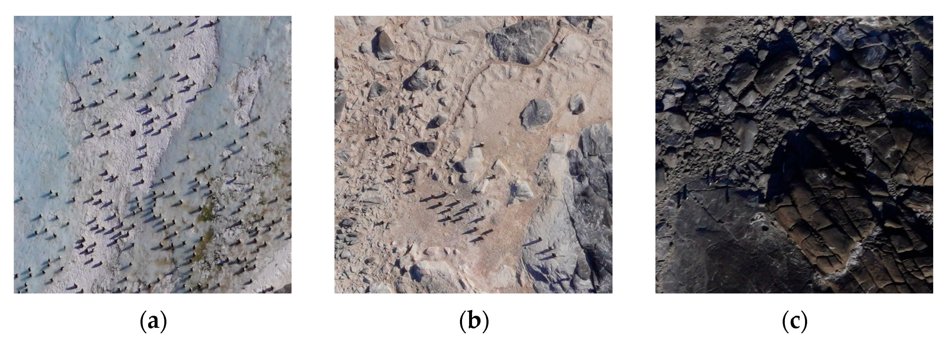
As shown in Figure 10, in white snow areas, small and densely distributed penguins can be detected commendably with almost no errors due to obvious aberration. According to statistics, the smallest penguin occupies three pixels. In the white rocks, though the shadow of penguin gets darker which may confuse with neighboring black penguins, YoloPd can still locate the two adjacent penguins. With the complexity of the terrain, penguins become increasingly invisible to human vision. As demonstrated in Figure 10c, penguins and their shadows can be highly similar to the background in shape and color around black rocks, even leading to missed detections by human vision. However, YoloPd can separate them that are hard to distinguish from black rocks. In particular, for the top image, some little rocks which have the same white color can be easily mistaken as penguins.
When analyzing the whole image prediction, it is important to consider both F1 and c o u n t i n g   a c c u r a c y comprehensively. To investigate the impact of C o n f t h r e on them, we select 20 thresholds within the range of [ 0.30 , 0.50 ] . As shown in Figure 11, the maximum c o u n t i n g   a c c u r a c y of 95.8% is achieved when C o n f t h r e = 0.33 , whereas the maximum F1 of 94.0% is observed at C o n f t h r e = 0.40 . Although large c o u n t i n g   a c c u r a c y is desirable, the false detections may lead to the inclusion of non-penguin object. On the other hand, F1 can better reflect the predicted number of real penguins. Therefore, we choose C o n f t h r e that corresponds to the highest F1 as the optimal choice. The other one is used as a measurement of feasibility for algorithms. When C o n f t h r e = 0.40 , 18 test images achieve 94.6% average c o u n t i n g   a c c u r a c y .
We select two different scenarios of the whole images to demonstrate the prediction results in Figure 12. For the densely distributed scene (a), small penguin pixel size and overlap with shadows lead to missed and false detections. Nevertheless, the F1 of this image can reach to 93.5%. In scenario (b) with sparse penguin distribution, the c o u n t i n g   a c c u r a c y is close to 99%.

4. Discussion

4.1. Method Comparison

To emphasize the advantage of our network in detecting penguins, we compare it with two SOTA methods Faster R-CNN and Yolov7. We select lightweight Backbones, ResNet-34 and ELANet-l, respectively, with similar Params. In order to show the advantage of Transformer, we also choose the smallest Backbone Swin-Transformer-tiny in Faster R-CNN. Besides, we select a stronger and larger Backbone ELANet-x as a contrast.
Firstly, as shown in Table 5 for the most classical detector Faster R-CNN, the Backbone Swin-Transformer shows better performance in accuracy than ResNet-34. Specifically, given a similar number of parameters, the former one improves F1, mAP.5, mAP by 1.3%, 1.3% and 1.8% respectively. However, the huge hardware overhead of Transformer leads to the reduction of FPS. When the more efficient Backbone ELANet-l is adopted in Yolov7, the F1 score is improved to 85.7% and achieves real-time detection performance with 66 FPS. By combining the advantages of both, our YoloPd outperforms Faster R-CNN (ResNet-34) by 6.2% F1, 8.5% mAP. Meanwhile, in contrast to the latest detector Yolov7, our hybrid structures provide performance gains with negligible inference speed degradation. YoloPd beats it by 2.3% F1, 2.1% mAP.5 and 1.9% mAP. Even compared to Yolov7 with the larger Backbone ELANet-x, the F1 is improved from 85.9% to 88.0% with 50.3% fewer parameters, achieving a good balance between accuracy and speed. We also show the visualized results of different methods in Figure 13.
Regarding the snow area (a), based on Faster R-CNN, the Backbone Swin-Transformer avoids a lot of false detections (penguins shadows) located by ResNet-34. From Refs. [28,50], this is likely due to the Transformer-based network’s ability to extract global features, enabling it to learn the difference between penguins and shadows. Additionally, Yolov7 with a stronger backbone is capable of extracting deeper features of objects, resulting in better classification accuracy. When combing both advantages, YoloPd can even detect penguins at the edges of the image correctly. Meanwhile, from the scene (b) we can see that Faster R-CNN demonstrates poor ability to detect densely distributed penguins. While equipped with the Yolo detector Head which is friendly for densely detections, YoloPd is able to reduce the number of missed penguins from 33 to five. In the complex scene (c), there exists small rocks that exhibit similar features to penguins. This can cause confusion for object detection models such as Faster R-CNN (ResNet-34), Faster R-CNN (Swin-Transformer) and Yolov7 (ELANet-l), which have mistaken five, two, and one rocks as penguins, respectively. In contrast, our network has managed to learn the subtle differences between the two, accurately detecting all penguins. Consequently, YoloPd achieves 100% F1 and c o u n t i n g   a c c u r a c y , proving to be the most effective model in this scenario.
In addition, according to our knowledge, there have been no papers published so far on using object detection algorithms to count penguins on the Antarctic islands because acquiring high resolution remote-sensing images is difficult due to their remote location. Compared to other indirect methods used for counting individuals such as Ref. [11] which uses a semantic segmentation technique that achieves a counting accuracy of 91%, our method has competitive indices. Besides, contrast to detect other animals, such as rabbits [46] and domestic cattle [47] with a counting accuracy of 95%, bird detection [48] with 90.63% mAP.5 and marine lives detection with an F1 of 79.7%, our results are remarkable. The new method initially meets the demand for correctly categorizing penguins, making this an exciting prospect for further research.

4.2. Ablation Experiments

To verify the effect of each of the improvements on the model performance, ablation experiments are conducted. For the sake of comparison, we treat BELAN and TBELAN as a unified entity BELAN during the experiment. We recorded F1, mAP.5, mAP, Params and FPS with different combination of MAConv, BELAN and AELAN based on Yolov7 (ELANet-l).
According to Table 6, we observe that the performance metrics vary when different modules are combined. However, not all combinations of modules can result in performance gains. For instance, we notice that adding the MAConv module leads to a 0.1% decrease in F1 score compared to using the AELAN module alone. This can be attributed to the fact that each improvement technique is not entirely independent, and sometimes combining the modules can be ineffective despite effective individual modules. Therefore, we have analyzed the results of the ablation experiments in the order of optimal network performance increment: Baseline + MAConv + BELAN + AELAN.
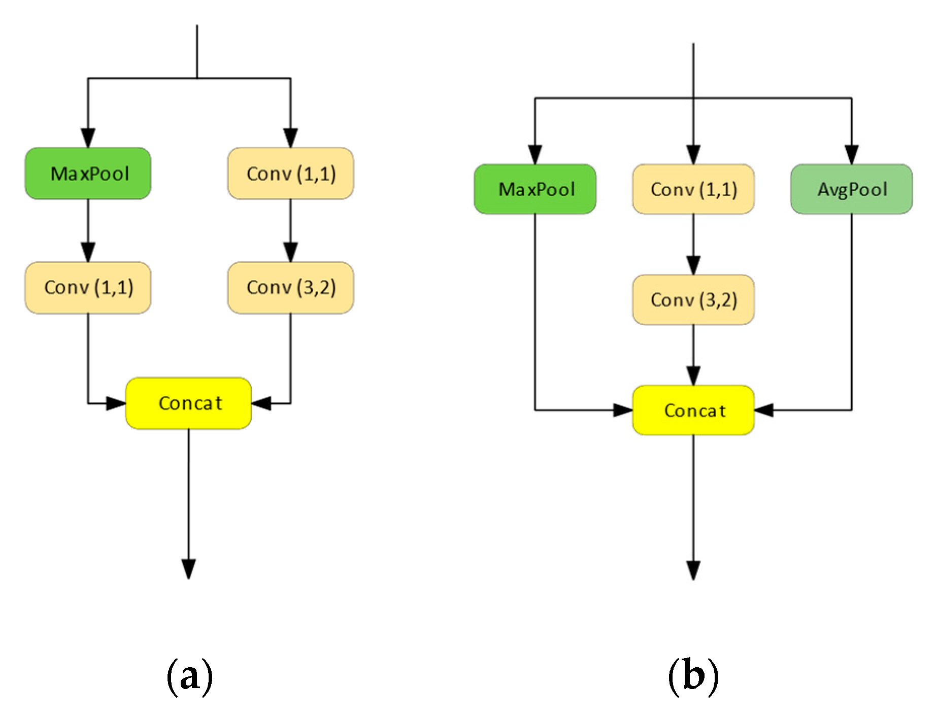
Baseline + MAConv: Firstly, we incorporate the multi-frequency attention fusion module MAConv in the down-sampling module of the entire network. By removing redundant convolutional layers, fusing multi-frequency information and avoiding information loss caused by small targets during down-sampling, we design a structure that slightly improves the network’s performance indicators while maintaining its speed.
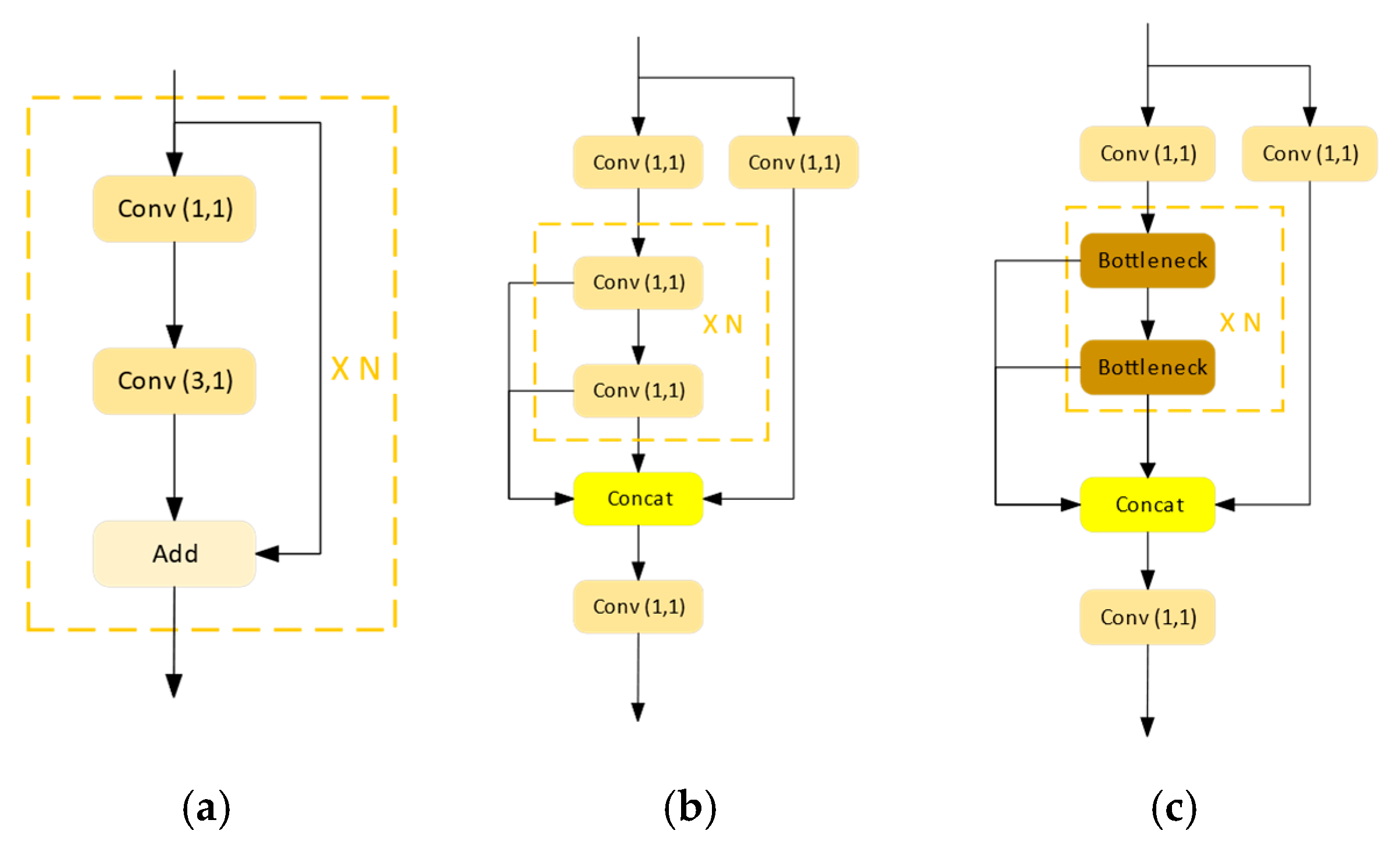
Baseline + MAConv + BELAN: Next, in the Backbone, we utilize the efficient Transformer and CNN hybrid module BELAN to extract more low-frequency features, significantly improving the network’s localization and classification capabilities. Compared to Yolov7, the incorporation of the two efficient modules improves F1, mAP.5, and mAP by 1.6%, 2.1% and 2.8%, respectively. However, the high computational cost of the Transformer reduces the inference speed of the network, resulting in a lowered FPS of 19.
Baseline + MAConv + BELAN + AELAN: Finally, we add the attention module AELAN in the Neck, which fuses multiscale features to produce an attention prediction feature map, further enhancing the network’s performance. Through these optimizations, we achieve an improved F1 of 88%, mAP.5 of 89.4 and mAP of 40.9 while striking a balance between speed and performance. Despite the loss of inference speed, the network maintained real-time inference performance at 43 FPS.
In conclusion, our proposed network with efficient modules showed improved performance in object detection while maintaining real-time inference speed. The incorporation of the MAConv, BELAN and AELAN modules contributed to the enhancement of the network’s performance in various aspects. Future work can focus on improving the network’s efficiency and performance further.

4.3. Exclusive Performance Comparison Experiments

In order to better demonstrate the advantages of YoloPd in recognizing smaller penguin compared to other SOTA method, we define T P R [ p , q ] to record the rate of detected penguins whose pixel size range in [ p , q ] to labeled penguins, it is calculated as following:
T P R [ p , q ] = P r e d n u m [ p , q ] G T n u m [ p , q ]
where P r e d n u m [ p , q ] and G T n u m [ p , q ] represent the number of predicted penguins that are true positive samples and labelled penguins, respectively. The pixel size is range in [ p , q ] .
As shown in Table 7, we conducted an experiment to compare the accuracy of Yolov7 (ELANet-l) and YoloPd in identifying penguins of different sizes. The former cannot recognize tiny penguins with pixels less than five, while YoloPd can accurately locate 4.8% of penguins that have been labelled. As pixels increase to 6–10, YoloPd outperforms Yolov7 in T P R [ p , q ] by 2% even though small penguins still provide limited information. When the pixel of the penguin is greater than 10, YoloPd can locate 98.6% of labelled penguins resulting in better recognition performance in detecting small objects. While YoloPd shows lower accuracy than Yolov7 in detecting larger penguins, it displays better average accuracy, which suggests that improving the detection performance of large objects could be a viable direction for subsequent optimization.
In addition, to evaluate our net’s ability of filtering out interference from complex backgrounds, we visualize the heat maps of the output feature ( P 3 ) from YoloPd and Yolov7 in Figure 14. From the three scenes with different backgrounds, it is apparent that YoloPd can rapidly capture penguin features and separate them from complex backgrounds. Specifically, in the white snow area (a), Yolov7 assigns more weight to cracks with color features similar to the penguins, while our network is able to accurately locate each penguin, resulting in higher recognition accuracy. In the rock areas (b) and (c), as previously mentioned, many black stones and their shadows have features extremely similar to the penguins, which confuses Yolov7’s ability to recognize them and leading to many false detections. However, YoloPd learns the global features of the interaction between penguin and their surroundings, thus greatly reducing the occurrence of missed and false detections. Furthermore, we also observed that when the background texture becomes more complex, such as having many scratched stones or cracked ice surfaces, YoloPd assigns relatively more attention to these backgrounds due to its ability of extracting low-frequency texture information. Fortunately, the attention weight of these backgrounds was much lower than that of the penguins we are interested in, so they could not significantly affect the detection performance.

4.4. Stability and Robustness Verification Experiments

As widely acknowledge, the quality of remote-sensing data is crucial to the recognition results. To ensure high-quality data, we employed the most advanced camera available. However, in the actual shooting process, external conditions such as camera, lighting and weather may significantly affect the quality of the captured images. To validate the stability of our proposed YoloPd, we follow the method in Ref. [38] and convolve the original images with Gaussian kernels of different sizes to simulate real-world situations to reduce the image quality. Specifically, we construct the blurred datasets by Gaussian kernels of sizes 3 × 3, 5 × 5 and 7 × 7. For clarity, we denote the original dataset as d a t a s e t _ o r i and the blurred dataset as d a t a s e t _ b l u r r y j , where j 3 , 5 , 7 , respectively, corresponding to different levels of blurriness.
We train them on Yolov7l and YoloPd as presented in Table 8. Our analysis reveals that as image quality deteriorates, Yolov7’s performance remains comparatively steady without any notable metric drop, whereas accuracy falls noticeable in YoloPd from validation set. Conversely, despite such shortcomings, YoloPd outperform yolov7 in terms of performance when tested on similar datasets. Results given in Figure 15, visualizing the effects of Gaussian Blur value, show that YoloPd can efficiently handle guillemot count requirements, as advancements in technology have significantly reduced the occurrence of images with low clarity levels. Moreover, our methodology leaves ample room for future improvements.
To evaluate the robustness of YoloPd and its ability to predict small targets from complex backgrounds, further experiments are conducted on other datasets. Since similar animal detection data are not publicly available and to ensure that the targets have similar sizes to penguins, we select the smallest category “small vehicle” in the DOTA dataset. The data processing followed the same procedure as the penguin detection dataset, where the images are cropped to a size of 640 × 640. A total of 9206 training set images and 2779 validation set images are obtained. Table 9 presents the experimental results of Yolov7 and YoloPd.
From results available it can be seen that YoloPd surpasses yolov7 by around 0.9% on F1 metric while demonstrating comparable mAP values. Although YoloPd doesn’t perform well for detecting cars as guillemots yet it possesses advantages in statistical smaller object counts. With respect to larger targets like discussed before. it may perform relatively lesser than Yolov7, but still satisfies our needs for counting penguins.
Meanwhile, it can be observed that our penguin detection dataset belongs to the category of small sample datasets, compared to the DOTA dataset, which has a training set of 9000 images. Generally speaking, networks trained on large datasets demonstrate enhanced robustness and accuracy on the same dataset, avoiding the problems of underfitting and overfitting. Fortunately, through careful selection, our validation set and training set have no overlap, achieving a better ratio of training set to validation set. This highlights the network’s adaptability to new scenarios, even with a smaller dataset. Therefore, overfitting is not a concern due to the smaller dataset size. Consequently, exploring methods to expand the dataset is also a direction for our future research.

5. Conclusions

In summary, our study showcases the effectiveness of automatic object detection in counting penguins from aerial remote-sensing images. Unlike traditional datasets, our dataset presents its own set of challenges, such as tiny penguins with intricate backgrounds. However, we are able to address these obstacles by introducing our novel object detection network, YoloPd, which is specifically designed to balance accuracy and speed. Our results show an impressive average counting accuracy of 94.6% across 18 images using YoloPd. This work highlights the potential of automatic object detection as a good automatic detection and identification tool for the Antarctic penguins. It can be used in practice to save human time, create new training data and establish initial, rapid population counts, with human verification of detected individuals as post-processing. Meanwhile, we also aim to apply our research to the study of species closely related to the Antarctic climate, such as seals, migratory birds and other organisms, with the commitment to accurately detect climate change and protect Antarctic wildlife.
However, there is still much potentials for improvement. Our dataset, in comparison to the commonly used remote-sensing dataset DOTA, is not sufficiently large to ensure solid interpretability. Therefore, further collection and annotation of penguin images is required, likely on a multi-year basis, to expand the dataset and improve accuracy as well as robustness. Additionally, improving the accuracy of large penguin detection is also a key optimization direction for us, so we can study the evolution of penguin distribution over time. Furthermore, investigation reveals that the number of active penguin nests has a significant impact on the population of penguins. Due to different data collection methods, we are unable to locate the position of nests from the images. In our future work, we aim to obtain high-quality, utilizing a combination of activate nest counting and individual counting methods to accurately detect population changes.

Author Contributions

Conceptualization, W.X. and J.H.; methodology, J.W. and W.X.; software, J.W.; validation, J.W., W.X., J.H. and M.L.; formal analysis, J.W., W.X., J.H. and M.L.; investigation, J.W.; resources, J.H. and M.L.; data curation, J.W. and M.L.; writing—original draft preparation, J.W.; writing—review and editing, J.W., W.X., J.H. and M.L.; visualization, J.W.; supervision, W.X. and M.L.; project administration, M.L. and J.H.; funding acquisition, W.X., J.H. and M.L. All authors have read and agreed to the published version of the manuscript.

Funding

This work is funded by the Program of Innovation 2030 on Smart Ocean, Zhejiang University (Grant No. 129000* 194232201, 129000 + 194432201); Impact and Response of Antarctic Seas to Climate Change (IRASCC NO. 22-01-02, 2022-02-02); Assessment of Polar Marine Ecosystems, Polar Research Institute of China (YW2022-01-01, YW2023-01-01).

Data Availability Statement

Due to contractual constraints with the Polar Research Institute of China and the unique nature of polar data, we regret that we are unable to share the raw aerial remote-sensing imagery freely.

Acknowledgments

We greatly appreciate the generous support by the Polar Research Institute of China for images to support this penguin counting project. Without their contributions, this work could not go ahead. Besides, we are also grateful to the Institute of Signal Space and Information, Zhejiang University for its technical and financial support.

Conflicts of Interest

The authors declare no conflict of interest.

References

  1. Turner, J.; Bindschadler, R.; Convey, P.; Di Prisco, G.; Fahrbach, E.; Gutt, J.; Hodgson, D.; Mayewski, P.; Summerhayes, C. Antarctic Climate Change and the Environment; SCAR: Cambridge, UK, 2009. [Google Scholar]
  2. Turner, J.; Marshall, G.J.; Clem, K.; Colwell, S.; Phillips, T.; Lu, H. Antarctic temperature variability and change from station data. Int. J. Climatol. 2020, 40, 2986–3007. [Google Scholar] [CrossRef]
  3. Lynch, H.J.; LaRue, M.A. First global census of the Adélie Penguin. Auk Ornithol. Adv. 2014, 131, 457–466. [Google Scholar] [CrossRef]
  4. Dias, M.P.; Warwick-Evans, V.; Carneiro, A.P.; Harris, C.; Lascelles, B.G.; Clewlow, H.L.; Manco, F.; Ratcliffe, N.; Trathan, P.N. Using habitat models to identify marine important bird and biodiversity areas for Chinstrap Penguins Pygoscelis antarcticus in the South Orkney Islands. Polar Biol. 2019, 42, 17–25. [Google Scholar] [CrossRef]
  5. Agnew, D.J. The CCAMLR ecosystem monitoring programme. Antarct. Sci. 1997, 9, 235–242. [Google Scholar] [CrossRef]
  6. Fretwell, P.T.; Trathan, P.N. Emperors on thin ice: Three years of breeding failure at Halley Bay. Antarct. Sci. 2019, 31, 133–138. [Google Scholar] [CrossRef]
  7. Mustafa, O.; Pfeifer, C.; Peter, H.U.; Kopp, M.; Metzig, R. Pilot study on monitoring climate-induced changes in penguin colonies in the Antarctic using satellite images. Proj. FKZ 2012, 3711, 199. [Google Scholar]
  8. Lynch, H.J.; Schwaller, M.R. Mapping the abundance and distribution of Adélie penguins using Landsat-7: First steps towards an integrated multi-sensor pipeline for tracking populations at the continental scale. PLoS ONE 2014, 9, e113301. [Google Scholar] [CrossRef]
  9. Witharana, C.; LaRue, M.A.; Lynch, H.J. Benchmarking of data fusion algorithms in support of earth observation based Antarctic wildlife monitoring. ISPRS J. Photogramm. Remote Sens. 2016, 113, 124–143. [Google Scholar] [CrossRef]
  10. Schwaller, M.R.; Olson, C.E., Jr.; Ma, Z.; Zhu, Z.; Dahmer, P. A remote sensing analysis of Adélie penguin rookeries. Remote Sens. Environ. 1989, 28, 199–206. [Google Scholar] [CrossRef]
  11. Le, H.; Samaras, D.; Lynch, H.J. A convolutional neural network architecture designed for the automated survey of seabird colonies. Remote Sens. Ecol. Conserv. 2022, 8, 251–262. [Google Scholar] [CrossRef]
  12. Fudala, K.; Bialik, R.J. The use of drone-based aerial photogrammetry in population monitoring of Southern Giant Petrels in ASMA 1, King George Island, maritime Antarctica. Glob. Ecol. Conserv. 2022, 33, e01990. [Google Scholar] [CrossRef]
  13. Shah, K.; Ballard, G.; Schmidt, A.; Schwager, M. Multidrone aerial surveys of penguin colonies in Antarctica. Sci. Robot. 2020, 5, eabc3000. [Google Scholar] [CrossRef]
  14. Bird, C.N.; Dawn, A.H.; Dale, J.; Johnston, D.W. A semi-automated method for estimating Adélie penguin colony abundance from a fusion of multispectral and thermal imagery collected with unoccupied aircraft systems. Remote Sens. 2020, 12, 3692. [Google Scholar] [CrossRef]
  15. Cheng, X.; Ji, M.; Zhang, B.; Zhang, Y.; Li, X. Sizing and trend analysis of penguin numbers in Antarctic from high resolution photography by unmanned aerial vehicle. J. Beijing Norm. Univ. 2019, 55, 25. [Google Scholar]
  16. Krizhevsky, A.; Sutskever, I.; Hinton, G.E. Imagenet classification with deep convolutional neural networks. Commun. ACM 2017, 60, 84–90. [Google Scholar] [CrossRef]
  17. Girshick, R.; Donahue, J.; Darrell, T.; Malik, J. Rich feature hierarchies for accurate object detection and semantic segmentation. In Proceedings of the IEEE Conference on Computer Vision and Pattern Recognition, Columbus, OH, USA, 23–28 June 2014; IEEE: Piscataway, NJ, USA, 2014; pp. 580–587. [Google Scholar]
  18. Girshick, R. Fast r-cnn. In Proceedings of the IEEE International Conference on Computer Vision, Santiago, Chile, 7–13 December 2015; IEEE: Piscataway, NJ, USA, 2015; pp. 1440–1448. [Google Scholar]
  19. Ren, S.; He, K.; Girshick, R.; Sun, J. Faster R-CNN: Towards Real-Time Object Detection with Region Proposal Networks. IEEE Trans. Pattern Anal. Mach. Intell. 2016, 39, 1137–1149. [Google Scholar] [CrossRef]
  20. Redmon, J.; Divvala, S.; Girshick, R.; Farhadi, A. You only look once: Unified, real-time object detection. In Proceedings of the IEEE Conference on Computer Vision and Pattern Recognition, Las Vegas, NV, USA, 27–30 June 2016; IEEE: Piscataway, NJ, USA, 2016; pp. 779–788. [Google Scholar]
  21. Redmon, J.; Farhadi, A. YOLO9000: Better, faster, stronger. In Proceedings of the IEEE Conference on Computer Vision and Pattern Recognition, Honolulu, HI, USA, 21–26 July 2017; IEEE: Piscataway, NJ, USA, 2017; pp. 7263–7271. [Google Scholar]
  22. Redmon, J.; Farhadi, A. Yolov3: An incremental improvement. arXiv 2018, preprint. arXiv:1804.02767. [Google Scholar]
  23. Bochkovskiy, A.; Wang, C.Y.; Liao, H.Y.M. Yolov4: Optimal speed and accuracy of object detection. arXiv 2020, arXiv:2004.10934. [Google Scholar]
  24. Jocher, G. YOLOv5 Release v6.1. Available online: https://github.com/ultralytics/yolov5/releases/tag/v6.2,2022.11 (accessed on 10 December 2022).
  25. Li, C.; Li, L.; Jiang, H.; Weng, K.; Geng, Y.; Li, L.; Ke, Z.; Li, Q.; Cheng, M.; Nie, W.; et al. YOLOv6: A single-stage object detection framework for industrial applications. arXiv 2022, arXiv:2209.02976. [Google Scholar]
  26. Wang, C.Y.; Bochkovskiy, A.; Liao, H.Y.M. YOLOv7: Trainable bag-of-freebies sets new state-of-the-art for real-time object detectors. arXiv 2022, arXiv:2207.02696. [Google Scholar]
  27. Dosovitskiy, A.; Beyer, L.; Kolesnikov, A.; Weissenborn, D.; Zhai, X.; Unterthiner, T.; Dehghani, M.; Minderer, M.; Heigold, G.; Gelly, S.; et al. An image is worth 16x16 words: Transformers for image recognition at scale. arXiv 2020, arXiv:2010.11929. [Google Scholar]
  28. Liu, Z.; Lin, Y.; Cao, Y.; Hu, H.; Wei, Y.; Zhang, Z.; Lin, S.; Guo, B. Swin transformer: Hierarchical vision transformer using shifted windows. In Proceedings of the IEEE/CVF International Conference on Computer Vision, Montreal, BC, Canada, 10–17 October 2021; IEEE: Piscataway, NJ, USA, 2021; pp. 10012–10022. [Google Scholar]
  29. Liu, Z.; Gu, X.; Chen, J.; Wang, D.; Chen, Y.; Wang, L. Automatic recognition of pavement cracks from combined GPR B-scan and C-scan images using multiscale feature fusion deep neural networks. Autom. Constr. 2023, 146, 104698. [Google Scholar] [CrossRef]
  30. Wang, D.; Liu, Z.; Gu, X.; Wu, W.; Chen, Y.; Wang, L. Automatic detection of pothole distress in asphalt pavement using improved convolutional neural networks. Remote Sens. 2022, 14, 3892. [Google Scholar] [CrossRef]
  31. Shi, P.; Jiang, Q.; Shi, C.; Xi, J.; Tao, G.; Zhang, S.; Zhang, Z.; Liu, B.; Gao, X.; Wu, Q. Oil Well Detection via Large-Scale and High-Resolution Remote Sensing Images Based on Improved YOLO v4. Remote Sens. 2021, 13, 3243. [Google Scholar] [CrossRef]
  32. Zhu, X.; Lyu, S.; Wang, X.; Zhao, Q. TPH-YOLOv5: Improved YOLOv5 based on transformer prediction head for object detection on drone-captured scenarios. In Proceedings of the IEEE/CVF International Conference on Computer Vision, Montreal, BC, Canada, 10–17 October 2021; IEEE: Piscataway, NJ, USA, 2021; pp. 2778–2788. [Google Scholar]
  33. Zhao, Q.; Liu, B.; Lyu, S.; Wang, C.; Zhang, H. TPH-YOLOv5++: Boosting Object Detection on Drone-Captured Scenarios with Cross-Layer Asymmetric Transformer. Remote Sens. 2023, 15, 1687. [Google Scholar] [CrossRef]
  34. Niu, R.; Zhi, X.; Jiang, S.; Gong, J.; Zhang, W.; Yu, L. Aircraft Target Detection in Low Signal-to-Noise Ratio Visible Remote Sensing Images. Remote Sens. 2023, 15, 1971. [Google Scholar] [CrossRef]
  35. Niu, R.; Zhi, X.; Jiang, S.; Gong, J.; Zhang, W.; Yu, L. Detector–Tracker Integration Framework for Autonomous Vehicles Pedestrian Tracking. Remote Sens. 2023, 15, 2088. [Google Scholar]
  36. Wu, J.; Shen, T.; Wang, Q.; Tao, Z.; Zeng, K.; Song, J. Local Adaptive Illumination-Driven Input-Level Fusion for Infrared and Visible Object Detection. Remote Sens. 2023, 15, 660. [Google Scholar] [CrossRef]
  37. Chen, Z.; Liu, C.; Filaretov, V.F.; Yukhimets, D.A. Multi-Scale Ship Detection Algorithm Based on YOLOv7 for Complex Scene SAR Images. Remote Sens. 2023, 15, 2071. [Google Scholar] [CrossRef]
  38. Van Etten, A. You only look twice: Rapid multi-scale object detection in satellite imagery. arXiv 2018, arXiv:1805.09512. [Google Scholar]
  39. Jian, L.; Pu, Z.; Zhu, L.; Yao, T.; Liang, X. SS R-CNN: Self-Supervised Learning Improving Mask R-CNN for Ship Detection in Remote Sensing Images. Remote Sens. 2022, 14, 4383. [Google Scholar] [CrossRef]
  40. Dong, X.; Qin, Y.; Gao, Y.; Fu, R.; Liu, S.; Ye, Y. Attention-Based Multi-Level Feature Fusion for Object Detection in Remote Sensing Images. Remote Sens. 2022, 14, 3735. [Google Scholar] [CrossRef]
  41. Kong, X.; Zhang, Y.; Tu, S.; Xu, C.; Yang, W. Vehicle Detection in High-Resolution Aerial Images with Parallel RPN and Density-Assigner. Remote Sens. 2023, 15, 1659. [Google Scholar] [CrossRef]
  42. Lin, T.Y.; Dollár, P.; Girshick, R.; He, K.; Hariharan, B.; Belongie, S. Feature pyramid networks for object detection. In Proceedings of the IEEE Conference on Computer Vision and Pattern Recognition; IEEE: Piscataway, NJ, USA, 2017; pp. 2117–2125. [Google Scholar]
  43. Duporge, I.; Isupova, O.; Reece, S.; Macdonald, D.W.; Wang, T. Using very-high-resolution satellite imagery and deep learning to detect and count African elephants in heterogeneous landscapes. Remote Sens. Ecol. Conserv. 2021, 7, 369–381. [Google Scholar] [CrossRef]
  44. Delplanque, A.; Foucher, S.; Lejeune, P.; Linchant, J.; Théau, J. Multispecies detection and identification of African mammals in aerial imagery using convolutional neural networks. Remote Sens. Ecol. Conserv. 2022, 8, 166–179. [Google Scholar] [CrossRef]
  45. Berg, P.; Santana Maia, D.; Pham, M.T.; Lefèvre, S. Weakly supervised detection of marine animals in high resolution aerial images. Remote Sens. 2022, 14, 339. [Google Scholar] [CrossRef]
  46. Ulhaq, A.; Adams, P.; Cox, T.E.; Khan, A.; Low, T.; Paul, M. Automated Detection of Animals in Low-Resolution Airborne Thermal Imagery. Remote Sens. 2021, 13, 3276. [Google Scholar] [CrossRef]
  47. Luo, W.; Zhang, Z.; Fu, P.; Wei, G.; Wang, D.; Li, X.; Shao, Q.; He, Y.; Wang, H.; Zhao, Z.; et al. Intelligent Grazing UAV Based on Airborne Depth Reasoning. Remote Sens. 2022, 14, 4188. [Google Scholar] [CrossRef]
  48. Hong, S.J.; Han, Y.; Kim, S.Y.; Lee, A.Y.; Kim, G. Application of deep-learning methods to bird detection using unmanned aerial vehicle imagery. Sensors 2019, 19, 1651. [Google Scholar] [CrossRef]
  49. Xia, G.S.; Bai, X.; Ding, J.; Zhu, Z.; Belongie, S.; Luo, J.; Datcu, M.; Pelillo, M.; Zhang, L. DOTA: A large-scale dataset for object detection in aerial images. In Proceedings of the IEEE Conference on Computer Vision and Pattern Recognition, Salt Lake City, UT, USA, 18–23 June 2018; IEEE: Piscataway, NJ, USA, 2018; pp. 3974–3983. [Google Scholar]
  50. Harris, C.M.; Herata, H.; Hertel, F. Environmental guidelines for operation of Remotely Piloted Aircraft Systems (RPAS): Experience from Antarctica. Biol. Conserv. 2019, 236, 521–531. [Google Scholar] [CrossRef]
  51. TzuTa Lin. LabelImg [Computer Software]. 2018. Available online: https://github.com/tzutalin/labelImg (accessed on 16 November 2022).
  52. Corbetta, M.; Shulman, G.L. Control of goal-directed and stimulus-driven attention in the brain. Nat. Rev. Neurosci. 2002, 3, 201–215. [Google Scholar] [CrossRef] [PubMed]
  53. Wang, F.; Jiang, M.; Qian, C.; Yang, S.; Li, C.; Zhang, H.; Wang, X.; Tang, X. Residual attention network for image classification. In Proceedings of the IEEE Conference on Computer Vision and Pattern Recognition, Honolulu, HI, USA, 21–26 July 2017; IEEE: Piscataway, NJ, USA, 2017; pp. 3156–3164. [Google Scholar]
  54. Hu, J.; Shen, L.; Sun, G. Squeeze-and-excitation networks. In Proceedings of the IEEE Conference on Computer Vision and Pattern Recognition, Salt Lake City, UT, USA, 18–23 June 2018; IEEE: Piscataway, NJ, USA, 2018; pp. 7132–7141. [Google Scholar]
  55. Park, N.; Kim, S. How do vision transformers work? arXiv 2022, arXiv:2202.06709. [Google Scholar]
  56. Jia, J.; Fu, M.; Liu, X.; Zheng, B. Underwater Object Detection Based on Improved EfficientDet. Remote Sens. 2022, 14, 4487. [Google Scholar] [CrossRef]
  57. Tan, M.; Pang, R.; Le, Q.V. Efficientdet: Scalable and efficient object detection. In Proceedings of the IEEE Conference on Computer Vision and Pattern Recognition, Seattle, WA, USA, 13–19 June 2020; IEEE: Piscataway, NJ, USA, 2020; pp. 10781–10790. [Google Scholar]
  58. Peng, Z.; Huang, W.; Gu, S.; Xie, L.; Wang, Y.; Jiao, J.; Ye, Q. Conformer: Local features coupling global representations for visual recognition. In Proceedings of the IEEE Conference on Computer Vision and Pattern Recognition, Nashville, TN, USA, 20–25 June 2021; IEEE: Piscataway, NJ, USA, 2021; pp. 367–376. [Google Scholar]
  59. Chen, Q.; Wu, Q.; Wang, J.; Hu, Q.; Hu, T.; Ding, E.; Cheng, J.; Wang, J. Mixformer: Mixing features across windows and dimensions. In Proceedings of the IEEE Conference on Computer Vision and Pattern Recognition, New Orleans, LA, USA, 18–24 June 2022; IEEE: Piscataway, NJ, USA; 2022; pp. 5249–5259. [Google Scholar]
  60. Li, J.; Xia, X.; Li, W.; Li, H.; Wang, X.; Xiao, X.; Wang, R.; Zheng, M.; Pan, X. Next-vit: Next generation vision transformer for efficient deployment in realistic industrial scenarios. arXiv 2022, arXiv:2207.05501. [Google Scholar]
  61. Li, Q.; Chen, Y.; Zeng, Y. Transformer with transfer CNN for remote-sensing-image object detection. Remote Sens. 2022, 14, 984. [Google Scholar] [CrossRef]
  62. Lu, S.; Liu, X.; He, Z.; Zhang, X.; Liu, W.; Karkee, M. Swin-Transformer-YOLOv5 for Real-Time Wine Grape Bunch Detection. Remote Sens. 2022, 14, 5853. [Google Scholar] [CrossRef]
  63. Woo, S.; Park, J.; Lee, J.Y.; Kweon, I.S. Convolutional block attention module. In Proceedings of the European Conference on Computer Vision (ECCV); Springer: Cham, Switzerland, 2018; pp. 3–19. [Google Scholar]
  64. Zheng, Z.; Wang, P.; Liu, W.; Li, J.; Ye, R.; Ren, D. Distance-IoU loss: Faster and better learning for bounding box regression. Proc. AAAI Conf. Artif. Intell. 2020, 34, 12993–13000. [Google Scholar] [CrossRef]
  65. Lin, T.Y.; Maire, M.; Belongie, S.; Hays, J.; Perona, P.; Ramanan, D.; Dollár, P.; Zitnick, C.L. Microsoft coco: Common objects in context. Computer Vision–ECCV 2014: 13th European Conference, Zurich, Switzerland, 6–12 September 2014, Proceedings, Part V 13; Springer International Publishing: New York, NY, USA, 2014; pp. 740–755. [Google Scholar]
Figure 1. Examples of aerial remote-sensing images taken over an island with Adelie penguins in Antarctica.
Remotesensing 15 02598 g001
Figure 2. The sub-images of our penguin detection datasets in three different back grounds: (a) snow field, (b) white rock area and (c) black rock area.
Remotesensing 15 02598 g002aRemotesensing 15 02598 g002b
Figure 3. The structure of modern object detectors. The M of Mx in the feature box represents the down-sampling times of input images. Bbox, class and score stand for the coordinate, class name and confidence of the detection box, specifically.
Remotesensing 15 02598 g003
Figure 4. YoloPd Structure. Conv (k,s) represents the convolution module with kernel size k and stride s. C i stands for feature maps of different scales. SPPCSP is an Attention module proposed in Yolov7. Modules Detect (P3-P5) is responsible for detecting small, medium and large penguins, respectively. MAConv, TBELAN-i and AELAN are proposed modules discussed in following.
Remotesensing 15 02598 g004
Figure 5. The structure of (a) AConv and (b) MAConv.
Remotesensing 15 02598 g005
Figure 6. The structure of (a) Bottleneck, (b) ELANet and (c) BELAN. N refers the number of modules.
Remotesensing 15 02598 g006
Figure 7. TBELAN module. LSViT represents the Lightweight Shifted-Window Vision Transformer module. BN represents Batch Normalization. LN stands for Layer Normalization. QKV are embeddings of input features.
Remotesensing 15 02598 g007
Figure 8. AELAN and CBAM module, where denotes element-wise multiplication, denotes element-wise addition, and Ⓢ denotes sigmoid function.
Remotesensing 15 02598 g008
Figure 9. The structure of RepConv in (a) training and (b) inference stage.
Remotesensing 15 02598 g009
Figure 10. Detection results for the selected penguin datasets in different backgrounds: (a) snow field, (b) white rock and (c) black rock. Each detected penguin is marked with a green box.
Remotesensing 15 02598 g010aRemotesensing 15 02598 g010b
Figure 11. F1- C o n f t h r e (blue) and counting accuracy- C o n f t h r e (red) curve.
Remotesensing 15 02598 g011
Figure 12. Example results of 9506 × 6336 image detection by YoloPd. The resolution of the sub-images shown in the figure is 2000 × 2000. (a) densely distributed and (b) sparse distributed areas. TPs, FPs, FNs and GTs (ground-truth) are marked as green, red, yellow and blue boxes, respectively.
Remotesensing 15 02598 g012
Figure 13. Visual detection results on Faster R-CNN, Yolov7 and YoloPd. (ac) denotes different backgrounds. TPs, FPs, FNs and GTs (ground-truth) are marked as green, red, yellow and blue boxes, respectively.
Remotesensing 15 02598 g013
Figure 14. Visual heat maps of the output features from Yolov7 and YoloPd with different backgrounds: (a) snow field, (b) white rock and (c) black rock. The darker the color (red), the higher the degree of attention that the network pays to it during the recognition process.
Remotesensing 15 02598 g014
Figure 15. Visual detection results of blurred datasets on YoloPd. TPs, FPs, FNs and GTs (ground-truth) are marked as green, red, yellow and blue boxes, respectively.
Remotesensing 15 02598 g015
Table 1. Sub-image statistics.
DatasetPositiveNegativeTotalPenguin Labels
Train1797450224733,436
Val1038260129820,058
Table 2. Statistics of the penguin pixel size.
1–5 Pixels6–10 Pixels11–20 Pixels21–50 Pixels
Train287151125,8205818
Val16383316,1512911
Table 3. Confusion Matrix. Prediction and Label represent detected and labeled boxes, respectively.
Label
PositiveNegative
PredictionPositiveTPFP
NegativeFNTN
Table 4. The number of BELAN and TBELAN-i modules.
BELANTBELAN-3TBELAN-4TBELAN-5
BottleneckLSViTBottleneckLSViTBottleneckLSViTBottleneckLSViT
30428222
Table 5. Comparison of different start-of-the-art methods on penguin detection. The unit of P, R, F1, mAP.5 and mAP are all %. Params’ unit is 10 6 .
MethodBackbone P R F 1 mAP.5mAPParamsFPS
Faster
R-CNN
ResNet-3487.776.681.878.432.438.420
Swin-Transformer-tiny88.878.183.179.734.244.813
Yolov7ELANet-l89.182.585.787.339.037.266
ELANet-x89.182.985.987.539.970.836
YoloPdBELANet90.785.588.089.440.935.243
Table 6. Network model performance for different combination modules. . indicates that the current module is used.
MAConvBELANAELANF1mAP.5mAPParamsFPS
85.787.339.037.266
86.488.340.238.061
87.089.040.535.048
86.888.940.637.257
87.389.440.835.247
86.788.840.138.153
87.789.941.435.041
88.089.440.935.243
Table 7. Comparison results of T P R [ p , q ] . The unit is %.
Method1–5 Pixels6–10 Pixels11–20 Pixels21–50 Pixels
Yolov7033.393.663.7
YoloPd4.835.398.662.0
Table 8. Comparison of datasets with different levels of blurriness on Yolov7 and YoloPd.
Method DatasetPRF1mAP.5mAP
Yolov7 d a t a s e t _ o r i 89.182.585.787.339.0
d a t a s e t _ b l u r r y 3 88.582.985.687.738.8
d a t a s e t _ b l u r r y 5 89.182.885.887.939.3
d a t a s e t _ b l u r r y 7 88.881.785.186.638.3
YoloPd d a t a s e t _ o r i 90.785.588.089.440.9
d a t a s e t _ b l u r r y 3 90.084.987.489.439.9
d a t a s e t _ b l u r r y 5 90.284.087.089.040.5
d a t a s e t _ b l u r r y 7 89.183.486.288.439.9
Table 9. Comparison results of small vehicle detection in DOTA on Yolov7 and YoloPd.
MethodPRF1mAP.5mAP
Yolov783.868.775.576.341.3
YoloPd83.670.476.476.541.2
Disclaimer/Publisher’s Note: The statements, opinions and data contained in all publications are solely those of the individual author(s) and contributor(s) and not of MDPI and/or the editor(s). MDPI and/or the editor(s) disclaim responsibility for any injury to people or property resulting from any ideas, methods, instructions or products referred to in the content.

