


DILRS: Domain-Incremental Learning for Semantic Segmentation in Multi-Source Remote Sensing Data

Abstract
: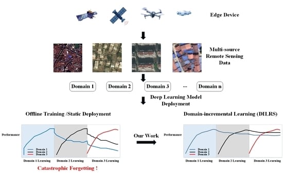
1. Introduction
- (1)
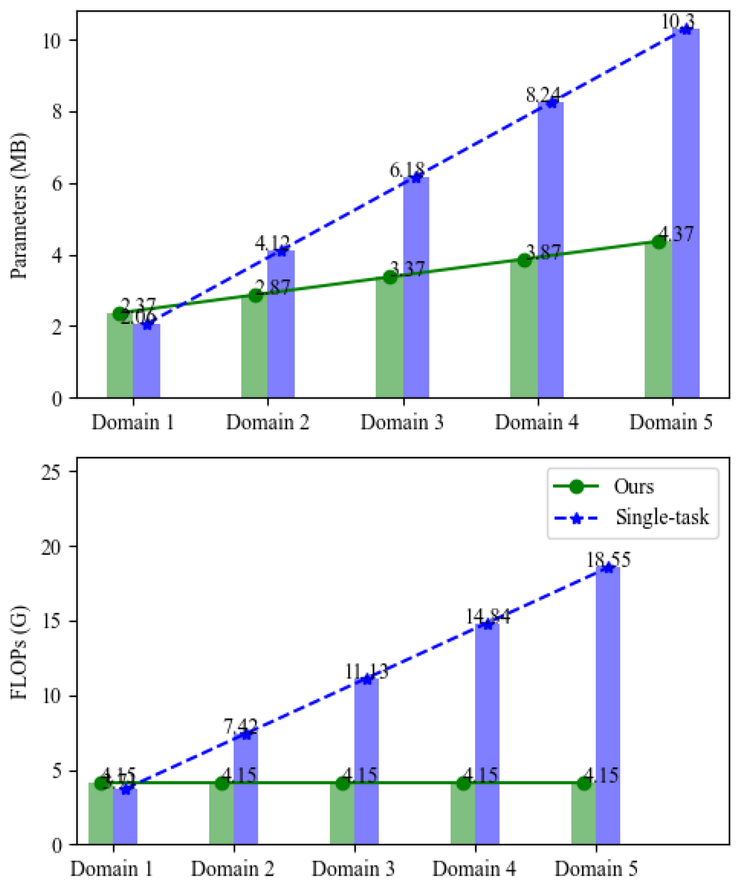
- We define the problem of domain-incremental learning for remote sensing and propose a dynamic framework specific for this problem without using previous training data and labels. Experimental results demonstrate the excellent performance of our method with fewer parameters.
- (2)
- To alleviate the domain shift among incremental domains, we adapt domain residual adapter modules in the structure, using different optimization strategies towards domain-specific and domain-agnostic parameters.
- (3)
- Consider different label space shift, class-specific knowledge distillation loss is applied to distil the common class knowledge between domains, and we also use the distillation loss at intermediate feature space to avoid background class interference.
2. Related Work
2.1. Incremental Learning
2.2. Domain-Incremental Learning
2.3. Incremental Learning for Semantic Segmentation
3. Method
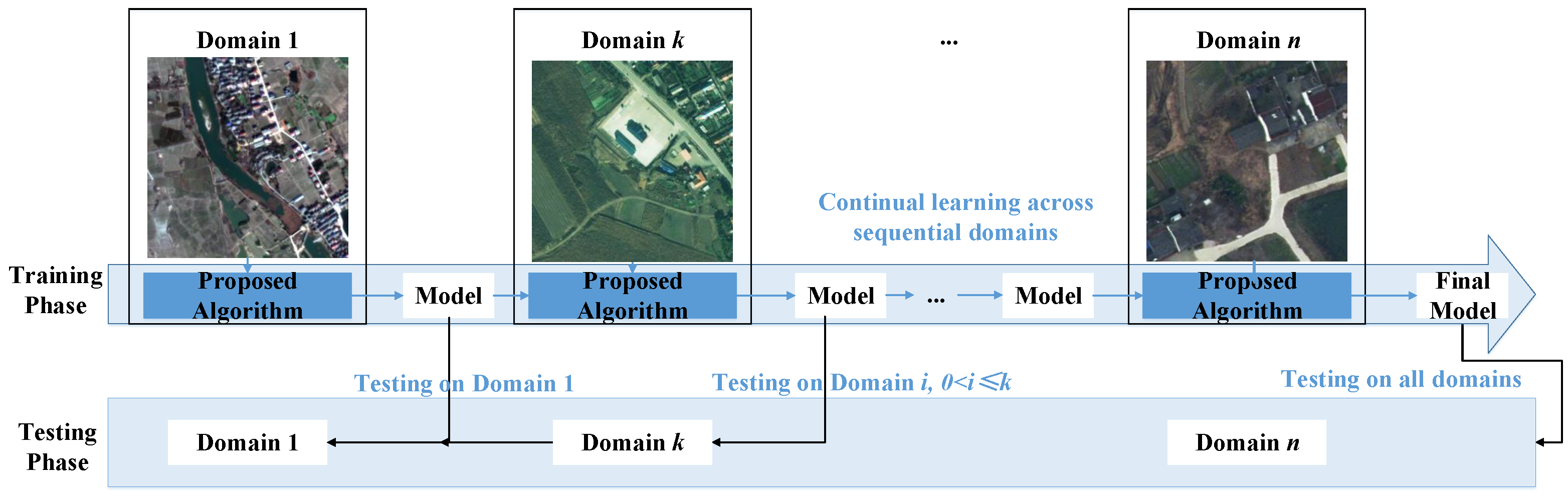
3.1. Problem Formulation
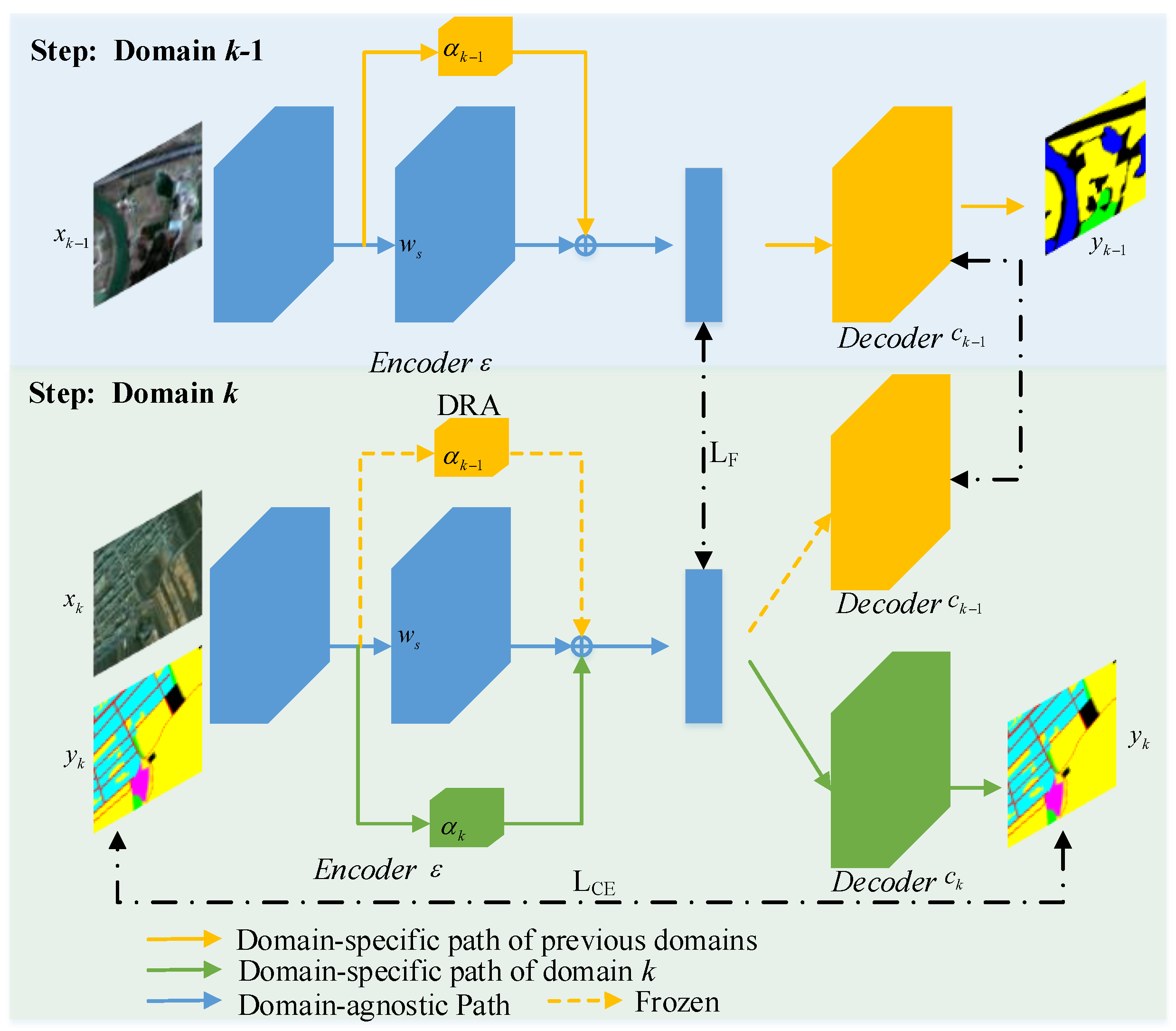
3.2. Proposed Framework
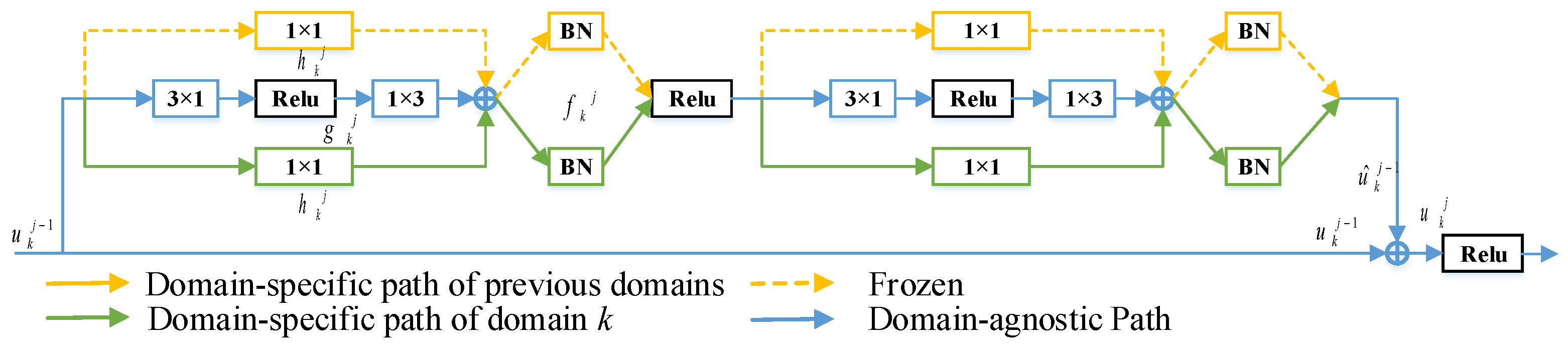
3.3. Domain Residual Adapter Module
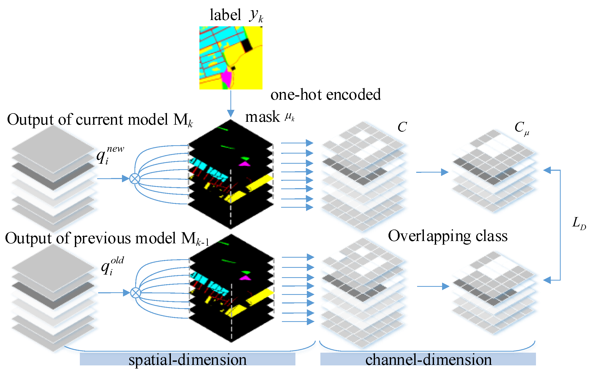
3.4. Loss
| Algorithm1: Process of learning a new domain of kth step in DILRS |
| Require: Dk: new domain (dataset) of current step k Mk−1: model of previous step k − 1 1: Initialization:Mk←add new domain-specific structure to Mk−1 initWk: Wk in Mk←Wk−1 in Mk−1 2: Freeze: domain-specific weights of all previous domains: Wi 3: for epochs do 4: Forward pass Mk(xk, k) via Wk 5: Compute cross-entropy loss LCE for Dk 6: Forward pass Mk(xk, k − 1) via Wk−1 7: Forward pass Mk−1(xk, k − 1) via Wk−1 8: Compute knowledge distillation loss LD, LF 9: Compute loss Ltotal 10: Update: Mk and Ms at learning rate lr 11: end for |
4. Experiments
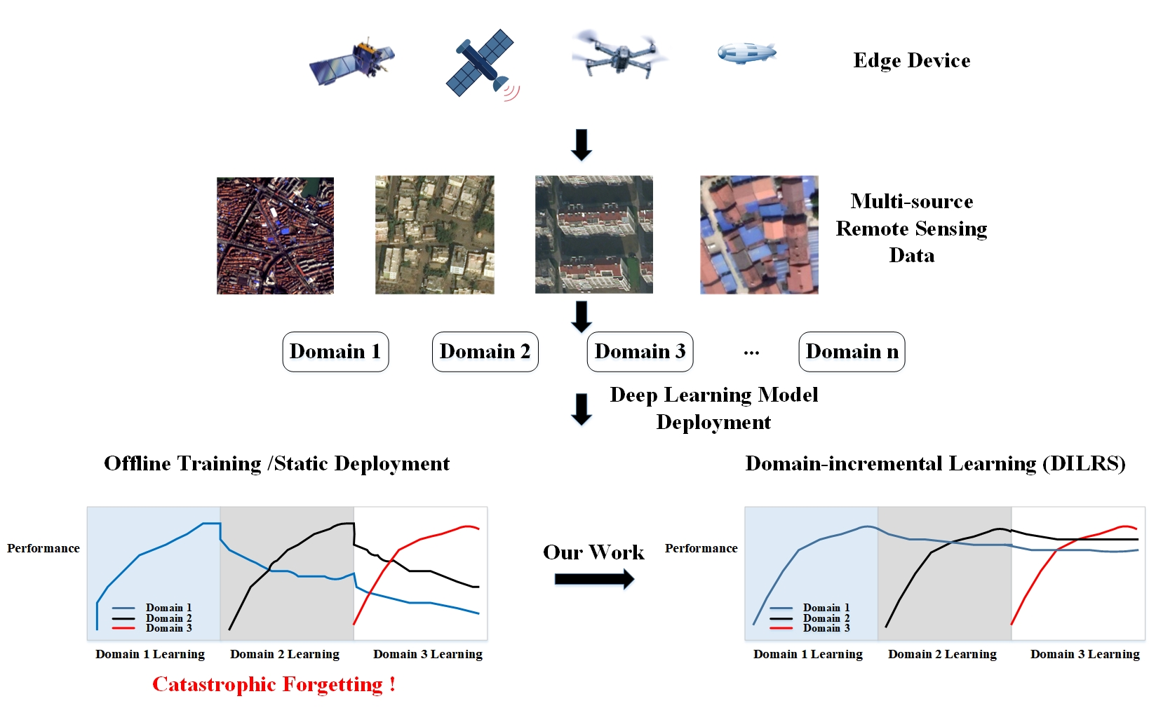
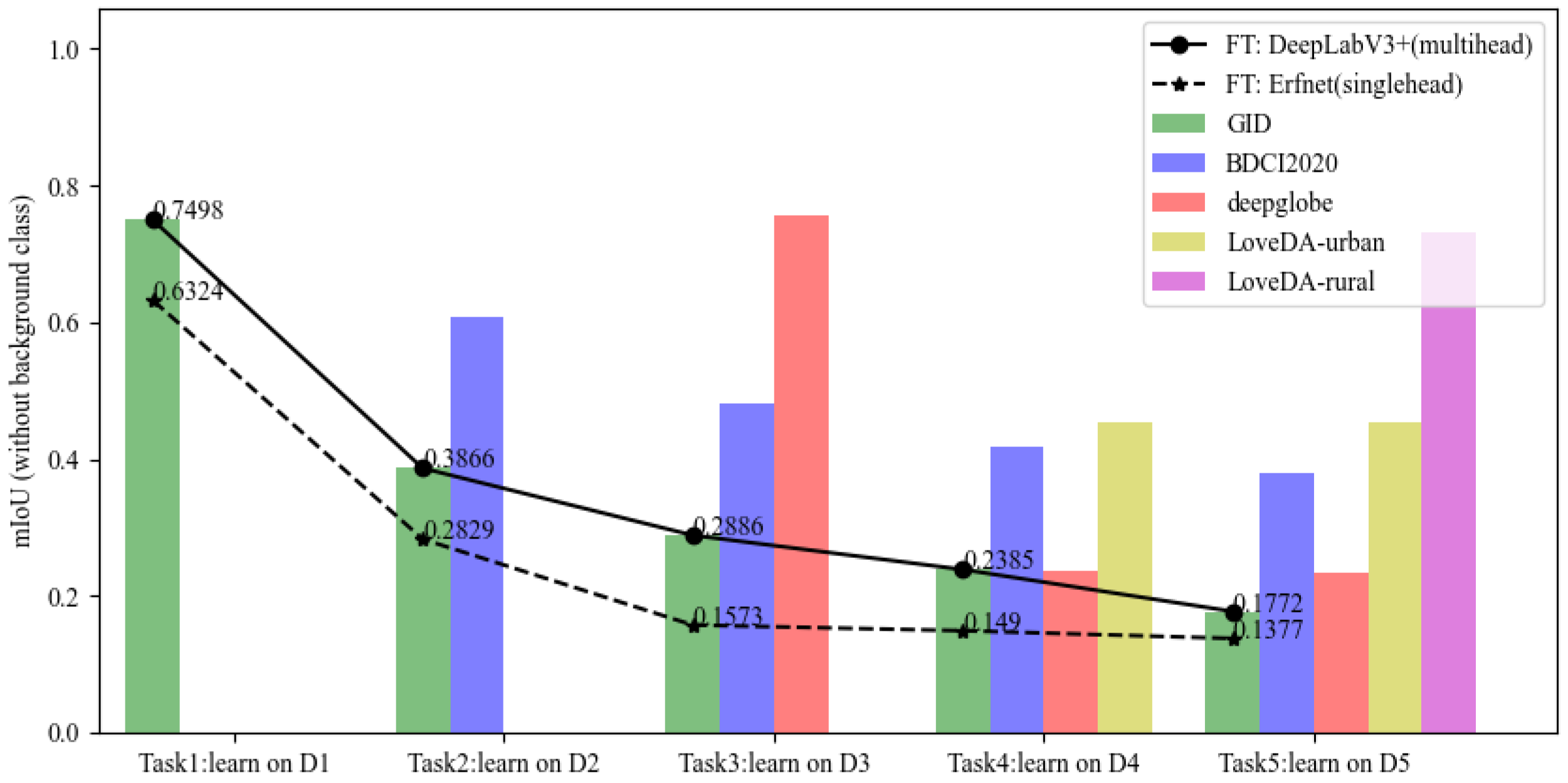
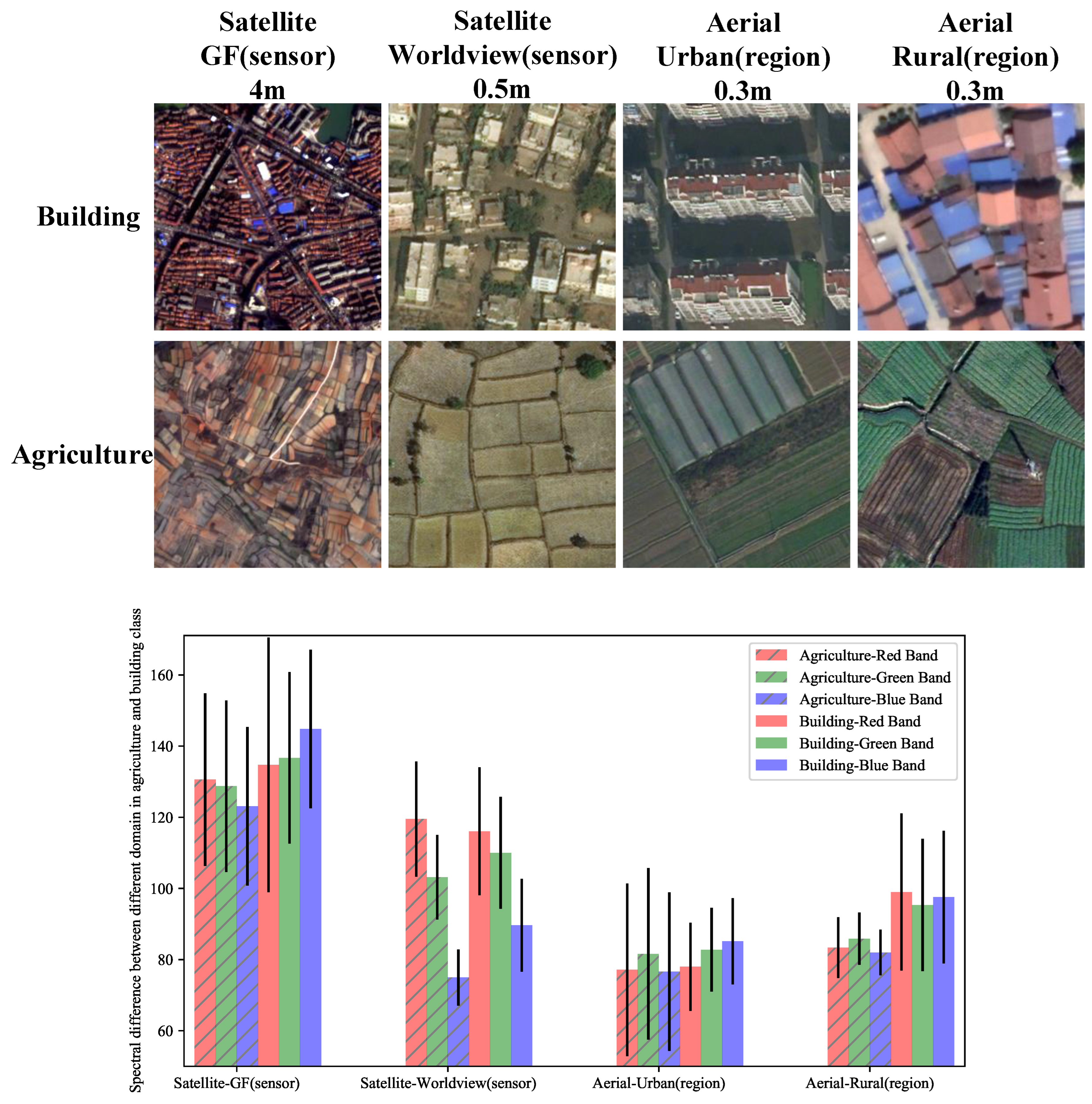
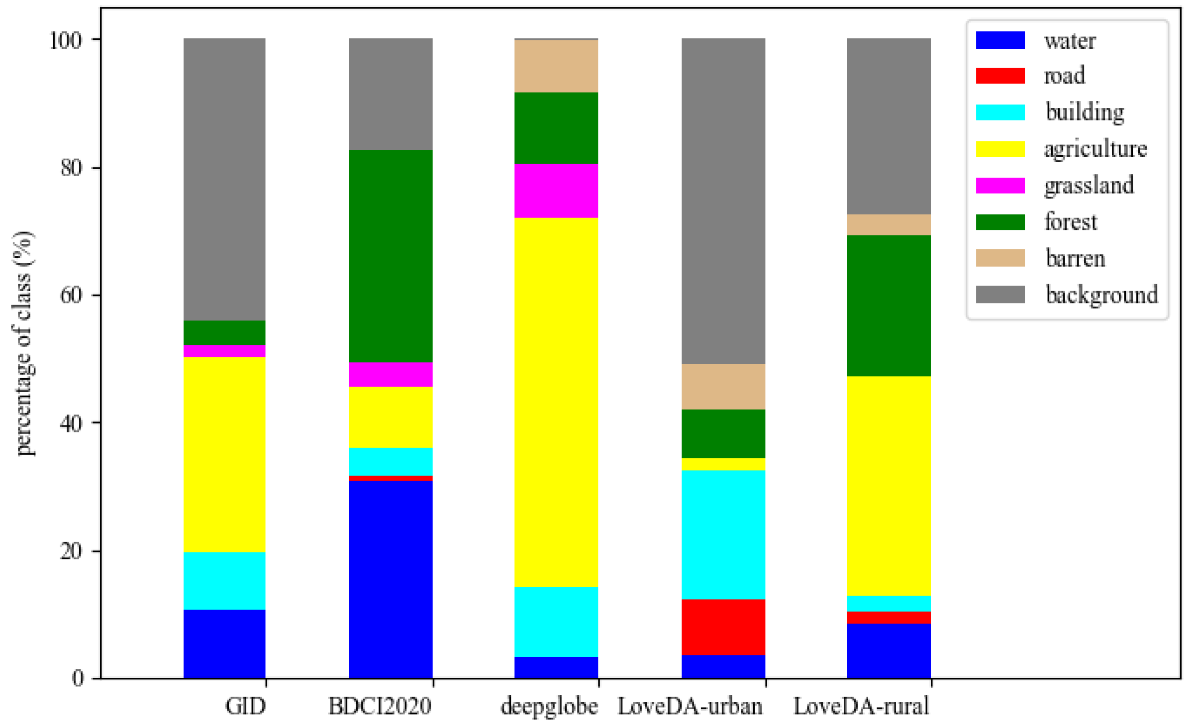
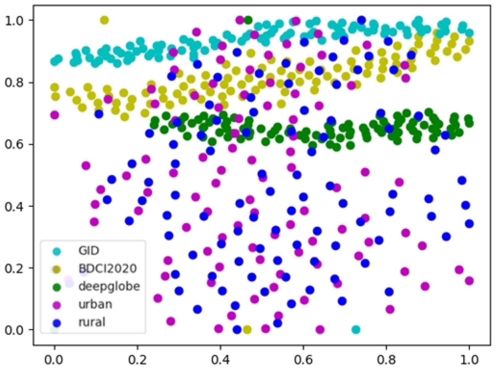
4.1. Datasets
4.2. Implementation Details
4.3. Compared Methods
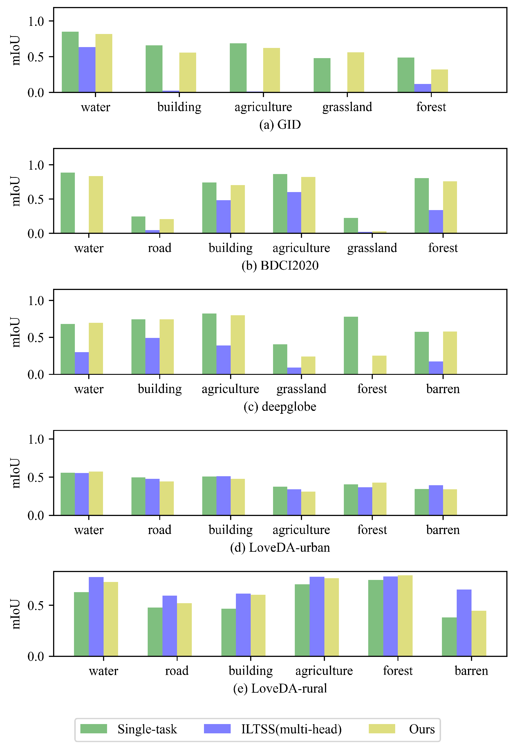
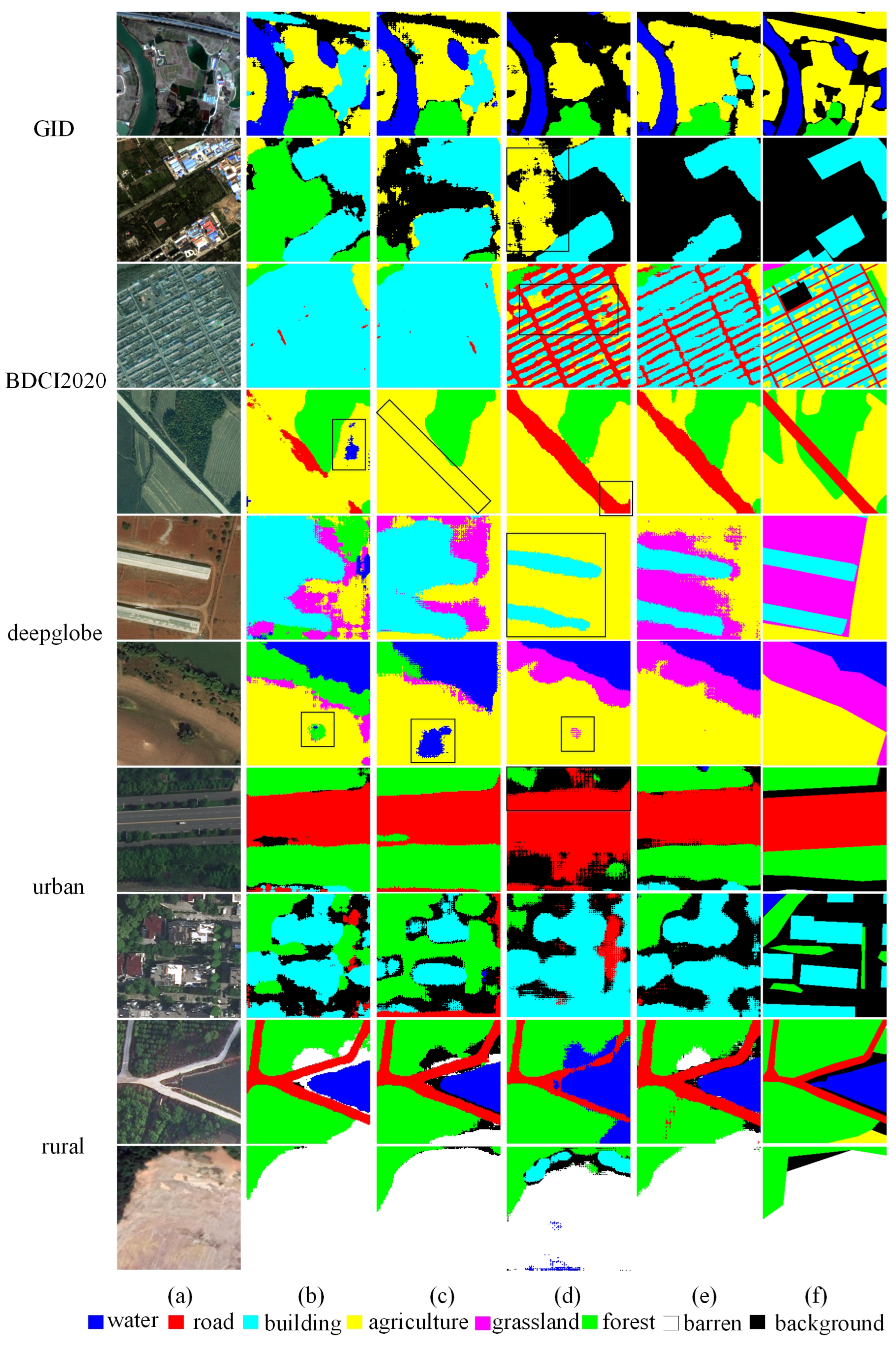
4.4. Experimental Results
4.5. Ablation Study
5. Conclusions
Author Contributions
Funding
Data Availability Statement
Conflicts of Interest
Abbreviations
| DRA | Domain residual adapter |
| DILRS | Domain-incremental learning for remote sensing |
| FT | Fine-tuning |
| FE | Feature extraction |
References
- Sun, X.; Liang, W.; Diao, W.; Cao, Z.Y.; Feng, Y.C.; Wang, B.; Fu, K. Progress and challenges of remote sensing edge intelligence technology. J. Image Graph. 2020, 25, 1719–1738. [Google Scholar] [CrossRef]
- Gan, Y.; Pan, M.; Zhang, R.; Ling, Z.; Zhao, L.; Liu, J.; Zhang, S. Cloud-Device Collaborative Adaptation to Continual Changing Environments in the Real-world. arXiv 2022, arXiv:2212.00972. [Google Scholar]
- Wang, Q.; Fink, O.; Van Gool, L.; Dai, D. Continual test-time domain adaptation. In Proceedings of the IEEE/CVF Conference on Computer Vision and Pattern Recognition, New Orleans, LA, USA, 18–24 June 2022; pp. 7201–7211. [Google Scholar]
- Chen, L.C.; Zhu, Y.; Papandreou, G.; Schroff, F.; Adam, H. Encoder-decoder with atrous separable convolution for semantic image segmentation. In Proceedings of the European Conference on Computer Vision (ECCV), Munich, Germany, 8–14 September 2018; pp. 801–818. [Google Scholar] [CrossRef]
- Romera, E.; Alvarez, J.M.; Bergasa, L.M.; Arroyo, R. Erfnet: Efficient residual factorized convnet for real-time semantic segmentation. IEEE Trans. Intell. Transport. Syst. 2017, 19, 263–272. [Google Scholar] [CrossRef]
- Li, Z.; Xia, P.; Rui, X.; Li, B. Exploring The Effect of High-frequency Components in GANs Training. ACM Trans. Multimed. Comput. Commun. Appl. 2023, 19, 1–22. [Google Scholar] [CrossRef]
- Li, Z.; Xia, P.; Tao, R.; Niu, H.; Li, B. A New Perspective on Stabilizing GANs Training: Direct Adversarial Training. IEEE Trans. Emerg. Top. Comput. Intell. 2023, 7, 178–189. [Google Scholar] [CrossRef]
- Mai, Z.; Li, R.; Jeong, J.; Quispe, D.; Kim, H.; Sanner, S. Online continual learning in image classification: An empirical survey. Neurocomputing 2022, 469, 28–51. [Google Scholar] [CrossRef]
- Van de Ven, G.M.; Tolias, A.S. Three scenarios for continual learning. arXiv 2019, arXiv:1904.07734. [Google Scholar] [CrossRef]
- Li, Z.; Wang, C.; Zheng, H.; Zhang, J.; Li, B. FakeCLR: Exploring Contrastive Learning for Solving Latent Discontinuity in Data-Efficient GANs. In Proceedings of the Computer Vision–ECCV 2022: 17th European Conference, Tel Aviv, Israel, 23–27 October 2022; Proceedings, Part XV. pp. 598–615. [Google Scholar]
- Li, Z.; Tao, R.; Wang, J.; Li, F.; Niu, H.; Yue, M.; Li, B. Interpreting the latent space of gans via measuring decoupling. IEEE Trans. Artif. Intell. 2021, 2, 58–70. [Google Scholar] [CrossRef]
- Li, Z.; Hoiem, D. Learning without forgetting. IEEE Trans. Pattern Anal. Machine Intell. 2017, 40, 2935–2947. [Google Scholar] [CrossRef]
- Tong, X.Y.; Xia, G.S.; Lu, Q.; Shen, H.; Li, S.; You, S.; Zhang, L. Land-cover classification with high-resolution remote sensing images using transferable deep models. Remote Sens. Environ. 2020, 237, 111322. [Google Scholar] [CrossRef]
- BDCI2020, C. Remote Sensing Image Segmentation Datatset. Available online: https://www.datafountain.cn/competitions/475 (accessed on 17 April 2022).
- Demir, I.; Koperski, K.; Lindenbaum, D.; Pang, G.; Huang, J.; Basu, S.; Hughes, F.; Tuia, D.; Raskar, R. Deepglobe 2018: A challenge to parse the earth through satellite images. In Proceedings of the IEEE Conference on Computer Vision and Pattern Recognition Workshops, Salt Lake City, UT, USA, 18–22 June 2018; pp. 172–181. [Google Scholar] [CrossRef]
- Wang, J.; Zheng, Z.; Ma, A.; Lu, X.; Zhong, Y. LoveDA: A Remote Sensing Land-Cover Dataset for Domain Adaptive Semantic Segmentation. arXiv 2021, arXiv:2110.08733. [Google Scholar] [CrossRef]
- Li, W.H.; Liu, X.; Bilen, H. Universal Representations: A Unified Look at Multiple Task and Domain Learning. arXiv 2022, arXiv:2204.02744. [Google Scholar]
- Liu, W.; Nie, X.; Zhang, B.; Sun, X. Incremental Learning With Open-Set Recognition for Remote Sensing Image Scene Classification. IEEE Trans. Geosci. Remote Sens. 2022, 60, 5622916. [Google Scholar] [CrossRef]
- Lu, X.; Sun, X.; Diao, W.; Feng, Y.; Wang, P.; Fu, K. LIL: Lightweight Incremental Learning Approach Through Feature Transfer for Remote Sensing Image Scene Classification. IEEE Trans. Geosci. Remote Sens. 2021, 60, 5611320. [Google Scholar] [CrossRef]
- Feng, Y.; Sun, X.; Diao, W.; Li, J.; Gao, X.; Fu, K. Continual learning with structured inheritance for semantic segmentation in aerial imagery. IEEE Trans. Geosci. Remote Sens. 2021, 60, 5607017. [Google Scholar] [CrossRef]
- Rong, X.; Sun, X.; Diao, W.; Wang, P.; Yuan, Z.; Wang, H. Historical Information-Guided Class-Incremental Semantic Segmentation in Remote Sensing Images. IEEE Trans. Geosci. Remote Sens. 2022, 60, 5622618. [Google Scholar] [CrossRef]
- Tasar, O.; Tarabalka, Y.; Alliez, P. Incremental learning for semantic segmentation of large-scale remote sensing data. IEEE J. Sel. Top. Appl. Earth Obs. Remote Sens. 2019, 12, 3524–3537. [Google Scholar] [CrossRef]
- Garg, P.; Saluja, R.; Balasubramanian, V.N.; Arora, C.; Subramanian, A.; Jawahar, C. Multi-Domain Incremental Learning for Semantic Segmentation. In Proceedings of the IEEE/CVF Winter Conference on Applications of Computer Vision, Waikoloa, HI, USA, 3–8 January 2022; pp. 761–771. [Google Scholar] [CrossRef]
- Rebuffi, S.A.; Bilen, H.; Vedaldi, A. Efficient parametrization of multi-domain deep neural networks. In Proceedings of the IEEE Conference on Computer Vision and Pattern Recognition, Salt Lake City, UT, USA, 18–23 June 2018; pp. 8119–8127. [Google Scholar] [CrossRef]
- Michieli, U.; Zanuttigh, P. Incremental learning techniques for semantic segmentation. In Proceedings of the IEEE/CVF International Conference on Computer Vision Workshops, Seoul, Republic of Korea, 27–28 October 2019. [Google Scholar] [CrossRef]
- Klingner, M.; Bär, A.; Donn, P.; Fingscheidt, T. Class-incremental learning for semantic segmentation re-using neither old data nor old labels. In Proceedings of the 2020 IEEE 23rd International Conference on Intelligent Transportation Systems (ITSC), Rhodes, Greece, 20–23 September 2020; pp. 1–8. [Google Scholar] [CrossRef]
- Cermelli, F.; Mancini, M.; Bulo, S.R.; Ricci, E.; Caputo, B. Modeling the background for incremental learning in semantic segmentation. In Proceedings of the IEEE/CVF Conference on Computer Vision and Pattern Recognition, Seattle, WA, USA, 13–19 June 2020; pp. 9233–9242. [Google Scholar] [CrossRef]
- Rebuffi, S.A.; Kolesnikov, A.; Sperl, G.; Lampert, C.H. icarl: Incremental classifier and representation learning. In Proceedings of the IEEE conference on Computer Vision and Pattern Recognition, Honolulu, HI, USA, 21–26 July 2017; pp. 2001–2010. [Google Scholar] [CrossRef]
- Kirkpatrick, J.; Pascanu, R.; Rabinowitz, N.; Veness, J.; Desjardins, G.; Rusu, A.A.; Milan, K.; Quan, J.; Ramalho, T.; Grabska-Barwinska, A.; et al. Overcoming catastrophic forgetting in neural networks. Proc. Natl. Acad. Sci. USA 2017, 114, 3521–3526. [Google Scholar] [CrossRef]
- Rajasegaran, J.; Hayat, M.; Khan, S.; Khan, F.S.; Shao, L. Random path selection for incremental learning. arXiv 2019, arXiv:1906.01120. [Google Scholar] [CrossRef]
- Rusu, A.A.; Rabinowitz, N.C.; Desjardins, G.; Soyer, H.; Kirkpatrick, J.; Kavukcuoglu, K.; Pascanu, R.; Hadsell, R. Progressive neural networks. arXiv 2016, arXiv:1606.04671. [Google Scholar] [CrossRef]
- Mirza, M.J.; Masana, M.; Possegger, H.; Bischof, H. An Efficient Domain-Incremental Learning Approach to Drive in All Weather Conditions. arXiv 2022, arXiv:2204.08817. [Google Scholar] [CrossRef]
- Lu, Y.; Wang, M.; Deng, W. Augmented Geometric Distillation for Data-Free Incremental Person ReID. In Proceedings of the IEEE/CVF Conference on Computer Vision and Pattern Recognition, New Orleans, LA, USA, 18–24 June 2022; pp. 7329–7338. [Google Scholar] [CrossRef]
- Gao, J.; Li, J.; Shan, H.; Qu, Y.; Wang, J.Z.; Zhang, J. Forget Less, Count Better: A Domain-Incremental Self-Distillation Learning Benchmark for Lifelong Crowd Counting. arXiv 2022, arXiv:2205.03307. [Google Scholar] [CrossRef]
- Wang, M.; Yu, D.; He, W.; Yue, P.; Liang, Z. Domain-incremental learning for fire detection in space-air-ground integrated observation network. Int. J. Appl. Earth Obs. Geoinf. 2023, 118, 103279. [Google Scholar] [CrossRef]
- Elshamli, A.; Taylor, G.W.; Areibi, S. Multisource domain adaptation for remote sensing using deep neural networks. IEEE Trans. Geosci. Remote Sens. 2019, 58, 3328–3340. [Google Scholar] [CrossRef]
- Wang, X.; Cai, Z.; Gao, D.; Vasconcelos, N. Towards universal object detection by domain attention. In Proceedings of the IEEE/CVF Conference on Computer Vision and Pattern Recognition, Long Beach, CA, USA, 15–20 June 2019; pp. 7289–7298. [Google Scholar] [CrossRef]
- Shan, L.; Wang, W.; Lv, K.; Luo, B. Class-incremental Learning for Semantic Segmentation in Aerial Imagery via Distillation in All Aspects. IEEE Trans. Geosci. Remote Sens. 2021, 60, 5615712. [Google Scholar] [CrossRef]
- Arnaudo, E.; Cermelli, F.; Tavera, A.; Rossi, C.; Caputo, B. A contrastive distillation approach for incremental semantic segmentation in aerial images. In Proceedings of the International Conference on Image Analysis and Processing, Lecce, Italy, 23–27 May 2022; pp. 742–754. [Google Scholar] [CrossRef]
- Michieli, U.; Zanuttigh, P. Continual semantic segmentation via repulsion-attraction of sparse and disentangled latent representations. In Proceedings of the IEEE/CVF Conference on Computer Vision and Pattern Recognition, Nashville, TN, USA, 20–25 June 2021; pp. 1114–1124. [Google Scholar] [CrossRef]
- Li, J.; Sun, X.; Diao, W.; Wang, P.; Feng, Y.; Lu, X.; Xu, G. Class-incremental learning network for small objects enhancing of semantic segmentation in aerial imagery. IEEE Trans. Geosci. Remote Sens. 2021, 60, 5612920. [Google Scholar] [CrossRef]
- Rebuffi, S.A.; Bilen, H.; Vedaldi, A. Learning multiple visual domains with residual adapters. Adv. Neural Inf. Process. Syst. 2017, 506–516. [Google Scholar] [CrossRef]
- Kanakis, M.; Bruggemann, D.; Saha, S.; Georgoulis, S.; Obukhov, A.; Gool, L.V. Reparameterizing convolutions for incremental multi-task learning without task interference. In Proceedings of the European Conference on Computer Vision, Glasgow, UK, 23–28 August 2020; pp. 689–707. [Google Scholar] [CrossRef]
- Hinton, G.; Vinyals, O.; Dean, J. Distilling the knowledge in a neural network. arXiv 2015, arXiv:1503.02531. [Google Scholar] [CrossRef]


| Dataset | Sensor | Resolution (m) | Image Width | Images | Classes |
|---|---|---|---|---|---|
| GID [13] | GF-2 | 4 | 256 | 109,201 | 6 (Water/Building/Agricultural/Forest/Grassland/Background) |
| BDCI2020 [14] | GF-1/6 | 2 | 256 | 145,982 | 7 (Water/Building/Agricultural/Forest/Grassland/Road/Background) |
| deepglobe [15] | WorldView-2 | 0.5 | 256 | 65,044 | 7 (Water/Building/Agricultural/Forest/Grassland/Barren/Background) |
| LoveDA-urban [16] | Airborne | 0.3 | 256 | 29,328 | 7 (Water/Building/Agricultural/Forest/Road/Barren/Background) |
| LoveDA-rural [16] | Airborne | 0.3 | 256 | 37,728 | 7 (Water/Building/Agricultural/Forest/Road/Barren/Background) |
| DIL Step | Step1 | Step2 | Step3 | Step4 | ||||||
|---|---|---|---|---|---|---|---|---|---|---|
| Methods | GID | GID | BDCI | GID | BDCI | Deepglobe | GID | BDCI | Deepglobe | Urban |
| Single-task | 0.6190 | 0.6190 | 0.6332 | 0.6190 | 0.6332 | 0.6226 | 0.6190 | 0.6332 | 0.6226 | 0.4312 |
| Multi-task | 0.6190 | 0.5526 (−0.0664) | 0.5666 | 0.4949 (−0.1241) | 0.5147 (−0.0520) | 0.5655 | 0.4194 (−0.1996) | 0.4084 (−0.1582) | 0.3722 (−0.1933) | 0.2674 |
| FT (single-head) | 0.6190 | 0.2512 (−0.3678) | 0.6365 | 0.1315 (−0.4875) | 0.2359 (−0.4006) | 0.6147 | 0.1555 (−0.4635) | 0.0901 (−0.5464) | 0.1002 (−0.5145) | 0.4126 |
| FE (multi-head) | 0.6190 | 0.6190 (ref) | 0.3034 | 0.6190 (ref) | 0.3034 (ref) | 0.1301 | 0.6190 (ref) | 0.3034 (ref) | 0.1301 (ref) | 0.2674 |
| EwC (single-head) [29] | 0.6190 | 0.2518 (−0.3672) | 0.6408 | 0.1736 (−0.4454) | 0.3034 (−0.3374) | 0.5172 | 0.1776 (−0.4414) | 0.1533 (−0.4875) | 0.1301 (−0.3871) | 0.3553 |
| LwF (single-head) [12] | 0.6443 | 0.4954 (−0.1489) | 0.5944 | 0.2863 (−0.3580) | 0.3127 (−0.2817) | 0.5827 | 0.2184 (−0.4258) | 0.1438 (−0.4506) | 0.1425 (−0.4402) | 0.3914 |
| LwF (multi-head) [12] | 0.6532 | 0.2538 (−0.3994) | 0.6074 | 0.1376 (−0.5156) | 0.1994 (−0.408) | 0.6362 | 0.1898 (−0.4634) | 0.0905 (−0.5169) | 0.0582 (−0.5779) | 0.4345 |
| ILTSS (single-head) [25] | 0.6532 | 0.2629 (−0.3903) | 0.5954 | 0.1531 (−0.5001) | 0.2067 (−0.3887) | 0.5902 | 0.1663 (−0.4869) | 0.1228 (−0.4726) | 0.1273 (−0.4629) | 0.4113 |
| ILTSS (multi-head) [25] | 0.6443 | 0.4347 (−0.2096) | 0.6217 | 0.2954 (−0.3489) | 0.3717 (−0.2499) | 0.6289 | 0.2213 (−0.4230) | 0.2625 (−0.3592) | 0.2331 (−0.3959) | 0.4307 |
| Ours | 0.6532 | 0.6510 (−0.0022) | 0.6064 | 0.6245 (−0.0287) | 0.5622 (−0.0442) | 0.6046 | 0.5530 (−0.1002) | 0.5694 (−0.0370) | 0.5398 (−0.0648) | 0.4306 |
| DIL step | Step5 | |||||||||
| Methods | GID | BDCI | deepglobe | urban | rural | |||||
| Single-task | 0.6190 | 0.6332 | 0.6226 | 0.4312 | 0.5467 | - | - | |||
| Multi-task | 0.4052 (−0.2138) | 0.3896 (−0.1770) | 0.4183 (−0.1472) | 0.2628 (−0.0046) | 0.4527 | −32.41 | 13.57 | |||
| FT (single-head) | 0.1560 (−0.4630) | 0.2069 (−0.4296) | 0.2404 (−0.3743) | 0.3845 (−0.0281) | 0.5701 | −42.01 | 32.37 | |||
| FE (multi-head) | 0.6190 (ref) | 0.3034 (ref) | 0.1301 (ref) | 0.2674 (ref) | 0.3102 | - | - | |||
| EwC (single-head) [29] | 0.2169 (−0.4021) | 0.3125 (−0.3283) | 0.2676 (−0.2497) | 0.3123 (−0.0430) | 0.5101 | −41.38 | 25.57 | |||
| LwF (single-head) [12] | 0.1861 (−0.4582) | 0.1181 (−0.4763) | 0.1295 (−0.4532) | 0.3282 (−0.0632) | 0.5539 | −50.61 | 36.27 | |||
| LwF (multi-head) [12] | 0.1887 (−0.4645) | 0.1980 (−0.4094) | 0.2463 (−0.3899) | 0.3678 (−0.0667) | 0.6543 | −38.74 | 33.26 | |||
| ILTSS (single-head) [25] | 0.1809 (−0.4723) | 0.1881 (−0.4073) | 0.2495 (−0.3407) | 0.3768 (−0.0345) | 0.6128 | −40.30 | 31.37 | |||
| ILTSS (multi-head) [25] | 0.2095 (−0.4348) | 0.2207 (−0.4010) | 0.2059 (−0.4230) | 0.4272 (−0.0035) | 0.6777 | −35.04 | 31.55 | |||
| Ours | 0.5601 (−0.0931) | 0.5507 (−0.0558) | 0.5248 (−0.0798) | 0.4180 (−0.0127) | 0.6233 | −5.46 | 6.03 | |||
| DIL Step | Single-Task | Single-Task | Step1 | Step2: Rural → Urban | Step1 | Step2: Urban → Rural | ||
|---|---|---|---|---|---|---|---|---|
| IoU per Category | Rural | Urban | Rural | Rural | Urban | Urban | Urban | Rural |
| mIoU | 0.4312 | 0.5467 | 0.4236 | 0.6091 (0.1855) | 0.5790 (0.1478) | 0.5280 | 0.5388 (0.0108) | 0.6945 (0.1477) |
| Water | 0.5569 | 0.6278 | 0.5054 | 0.7677 (0.2623) | 0.6976 (0.1407) | 0.6175 | 0.5866 (−0.0309) | 0.7517 (0.1239) |
| Road | 0.4947 | 0.4771 | 0.3039 | 0.5240 (0.2201) | 0.5375 (0.0428) | 0.5457 | 0.5421 (−0.0036) | 0.5763 (0.0992) |
| Building | 0.5056 | 0.4667 | 0.3278 | 0.5511 (0.2233) | 0.5948 (0.0892) | 0.5637 | 0.5535 (−0.0102) | 0.6241 (0.1574) |
| Agriculture | 0.3722 | 0.7042 | 0.4491 | 0.4959 (0.0468) | 0.7006 (0.3284) | 0.3332 | 0.3051 (−0.0281) | 0.8266 (0.1224) |
| Forest | 0.4026 | 0.7480 | 0.1710 | 0.4471 (0.2761) | 0.6756 (0.2730) | 0.3662 | 0.4360 (0.0698) | 0.8332 (0.0852) |
| Barren | 0.3434 | 0.3815 | 0.2444 | 0.4507 (0.2063) | 0.4702 (0.1268) | 0.3864 | 0.3752 (−0.0112) | 0.6386 (0.2571) |
| 1 | √ | −33.12 | 26.46 | |||
| 2 | √ | √ | −15.25 | 15.21 | ||
| 3 | √ | √ | −9.24 | 11.44 | ||
| 4 | √ | √ | −10.01 | 14.04 | ||
| 5 | √ | √ | √ | −5.46 | 6.03 |
| 10.1 | −7.45 | 8.48 |
| 11 | −5.46 | 6.03 |
| 110 | −27.75 | 24.19 |
| 1100 | −32.41 | 13.57 |
Disclaimer/Publisher’s Note: The statements, opinions and data contained in all publications are solely those of the individual author(s) and contributor(s) and not of MDPI and/or the editor(s). MDPI and/or the editor(s) disclaim responsibility for any injury to people or property resulting from any ideas, methods, instructions or products referred to in the content. |
© 2023 by the authors. Licensee MDPI, Basel, Switzerland. This article is an open access article distributed under the terms and conditions of the Creative Commons Attribution (CC BY) license (https://creativecommons.org/licenses/by/4.0/).
Share and Cite
Rui, X.; Li, Z.; Cao, Y.; Li, Z.; Song, W. DILRS: Domain-Incremental Learning for Semantic Segmentation in Multi-Source Remote Sensing Data. Remote Sens. 2023, 15, 2541. https://doi.org/10.3390/rs15102541
Rui X, Li Z, Cao Y, Li Z, Song W. DILRS: Domain-Incremental Learning for Semantic Segmentation in Multi-Source Remote Sensing Data. Remote Sensing. 2023; 15(10):2541. https://doi.org/10.3390/rs15102541
Chicago/Turabian StyleRui, Xue, Ziqiang Li, Yang Cao, Ziyang Li, and Weiguo Song. 2023. "DILRS: Domain-Incremental Learning for Semantic Segmentation in Multi-Source Remote Sensing Data" Remote Sensing 15, no. 10: 2541. https://doi.org/10.3390/rs15102541