Article

Trends of Aboveground Net Primary Productivity of Patagonian Meadows, the Omitted Ecosystem in Desertification Studies

by
Matías Curcio
1,2,
Gonzalo Irisarri
3,4,*,
Guillermo García Martínez
2 and
Martín Oesterheld
4
1
Consejo Nacional de Investigaciones Científicas y Técnicas (CONICET), Godoy Cruz 2290, Argentina
2
Instituto Nacional de Tecnología Agropecuaria (INTA), Chacabuco 513, Esquel Chubut 9200, Argentina
3
Net Zero & Resilient Farming Directorate, Rothamsted Research, North Wyke, Devon EX20 2SB, UK
4
Instituto de Investigaciones Fisiológicas y Ecológicas Vinculadas a la Agricultura (IFEVA), Facultad de Agronomía, Universidad de Buenos Aires—CONICET, Buenos Aires 1428, Argentina
*
Author to whom correspondence should be addressed.
Remote Sens. 2023, 15(10), 2531; https://doi.org/10.3390/rs15102531
Submission received: 21 March 2023 / Revised: 22 April 2023 / Accepted: 8 May 2023 / Published: 11 May 2023
(This article belongs to the Special Issue Land Degradation Assessment with Earth Observation (Second Edition))

Abstract

:
The United Nations defines desertification as the loss of productivity in arid and semiarid environments. The extended steppes of Patagonia harbor small meadows whose compounded area is comparatively small, but their aboveground net primary production (ANPP) is up to ten times higher than their surroundings. These meadows then represent a key ecosystem for cattle grazing systems, but there are no descriptions of the trends in their ANPP and, consequently, their carrying capacity, and, as a result, their degradation syndromes. Our objectives were as follows: (1) analyze the trends of mean and spatial heterogeneity of annual ANPP in meadows and neighboring steppes and relate them with precipitation and temperature, (2) evaluate the impact on the livestock carrying capacity of meadows in the region, and (3) evaluate the degradation trends of these meadows, based on a novel description proposed to characterize the trend syndromes of these type of ecosystems. We identified meadow areas across a subcontinental scale in Patagonia, covering a mean annual precipitation range from 129 to 936 mm. We estimated ANPP on a monthly basis from 2000 to 2019 via regional calibrated remote sensing information. In the last two decades, ANPP decreased in 74% of the studied meadow areas, while remaining relatively stable in the nearby steppes. This decrease was relatively higher in the arid end of the analyzed precipitation gradient. Hence, the global carrying capacity for all the studied meadow areas decreased by 8%. Finally, we identified four trend syndromes based on the combination of the ANPP trend and its spatial heterogeneity, calculated as the spatial standard deviation. The predominant trend syndrome, in 55% of the area, was associated with a negative trend of both ANPP and spatial heterogeneity. These results could help prioritize areas where specific management decisions, given the different trend syndromes, could help revert ANPP negative trends.

1. Introduction

Wetlands situated in arid zones are fundamental as a carbon sink [1], partially because of their high productivity [2]. However, because of direct human disturbance and climate change, they are prone to desertification and a reduction in productivity over time [3], which can lead to the loss of wetland areas [4]. Patagonian meadows, locally named ‘‘mallines’’ or “vegas”, are a case of wetland inserted in an arid and semi-arid matrix [5,6], although they are also found in areas with a humid climate and oceanic characteristics in the extreme south of the region [7,8]. These meadows experience large seasonal fluctuations in the groundwater table, including flooded conditions during winter and early spring [9]. This implies a greater relative availability of water with respect to the surrounding steppe, which also leads to an aboveground net primary productivity (ANPP) that can be up to ten times higher than in the steppes [10,11,12]. Additionally, they exhibit a high internal heterogeneity of ANPP associated with the groundwater table depth from the more xeric peripheral environments (generally with the groundwater table at greater depths) to the more central humid parts, where the ANPP can vary from 2000 to 10,000 kg/ha.yr, respectively [10,11,12,13]. Even though meadows represent less than 5% of the Patagonian region [14,15], they are key to the development and sustainability of rural environments [5,14,16]. They are an essential source of forage feed [10,11,12,17,18], and consequently, they are key determinants of the animal carrying capacity [19]. Within the last twenty years, there has been an increasing amount of evidence indicating negative trends of ANPP across vast areas of Patagonia [10,20,21,22,23], where trends exhibited localized clusters [20,21]. However, three aspects remain poorly understood. First, the descriptions for Patagonia were carried out without discriminating meadows from the surrounding steppes. Therefore, potential ANPP trends in meadows are unknown, and it is unclear if they resemble those of steppes. Second, consequently, there are no regional descriptions of the change in the carrying capacity of meadows. Third, and beyond the meadows of Patagonia, we lack a conceptual framework to compare the trend syndromes of meadows.
Potentially, meadows may be more vulnerable to adverse climatic conditions, such as drought and or high heat events, given that the availability of water depends on the excesses of precipitation that congregate within the watershed that contains them. Two potential and related mechanisms might provoke negative trends of ANPP. First, the surrounding steppe soils exhibit a maximum water-holding capacity that is lower than the mean annual precipitation [24], partially because annual precipitation is concentrated in the winter period [25]. The winter excesses of water accumulate at the lower portions of the landscape where meadows are located [6]. If there are shifts in the seasonality of precipitation, from the winter to the spring, and/or decreases in the amount of precipitation over time, as observed in some areas of Patagonia [26], then the steppes area might not experience negative shifts in the water storage, or they might be mild. However, this might affect the water that congregates in the lower portions of the landscape, potentially decreasing the water table depth and affecting meadow plants’ access to water. Moreover, there are positive temperature trends in vast areas of Patagonia [23]. These temperature trends affected both positive and negative ANPP within the beginning of the growing season of meadows [27]. Less clear is the impact of this trend on the annual ANPP for both meadow areas and the nearby steppes. Increases in temperature can lead to increases in water demand, depleting water levels earlier, and decreases in ANPP, with different relative effects on meadows compared to nearby steppe areas. Furthermore, it is unknown if the potential ANPP trends are greater in more xeric environments compared to more humid ones.
On top of the climate effect on meadow’s ANPP trends are the potential effects of different management practices. Within Patagonia, sheep grazing is the most extended land use [19,28]. In this context, meadows are prone to interventions that seek to revert degradation processes [29]. Overgrazing by both domestic and native herbivores can decrease vegetation cover, which induces a higher evaporative rate of the soil and intensifies erosion and salinization processes [30]. If this process persists over time and is accelerated by adverse climatic conditions, it can lead to irreversible conditions [31,32]. Furthermore, the courses that provided water within a meadow begin to erode, producing gullies and acting as a drainage network [31]. During this process, it is expected that meadows’ mean ANPP will decrease over time and that its heterogeneity will, first, increase, given by patches of high and low ANPP. This increase in heterogeneity would be due to the existence of areas that dried up and others that still did not. However, if meadows’ watercourses continue to erode, there might be an irreversible shift, a tipping point [33,34], where ANPP keeps decreasing but is different from the previous phase; here, ANPP heterogeneity decreases as well. Landscape management practices may be implemented to avoid reaching such tipping points. Actions to redistribute and preserve the available water [29] should improve meadows’ productivity, avoiding the turn to an irreversible negative trend. Capturing these trends across meadows would deepen the understanding of these ecosystems functioning before capturing their loss of area [4].
Our main objective was to quantify the degradation trends of meadows across Patagonia through ANPP trends. Furthermore, we compared these trends with those in surrounding steppes and related their trends with environmental controls. Therefore, we addressed the following three specific objectives: (1) analyze the trends of mean and spatial heterogeneity of annual ANPP in meadows and neighboring steppes and relate them with precipitation and temperature, (2) evaluate the impact on the livestock carrying capacity of meadows in the region, and (3) evaluate the degradation trends of these meadows, based on a novel description proposed to characterize the trend syndromes of these type of ecosystems.

2. Materials and Methods
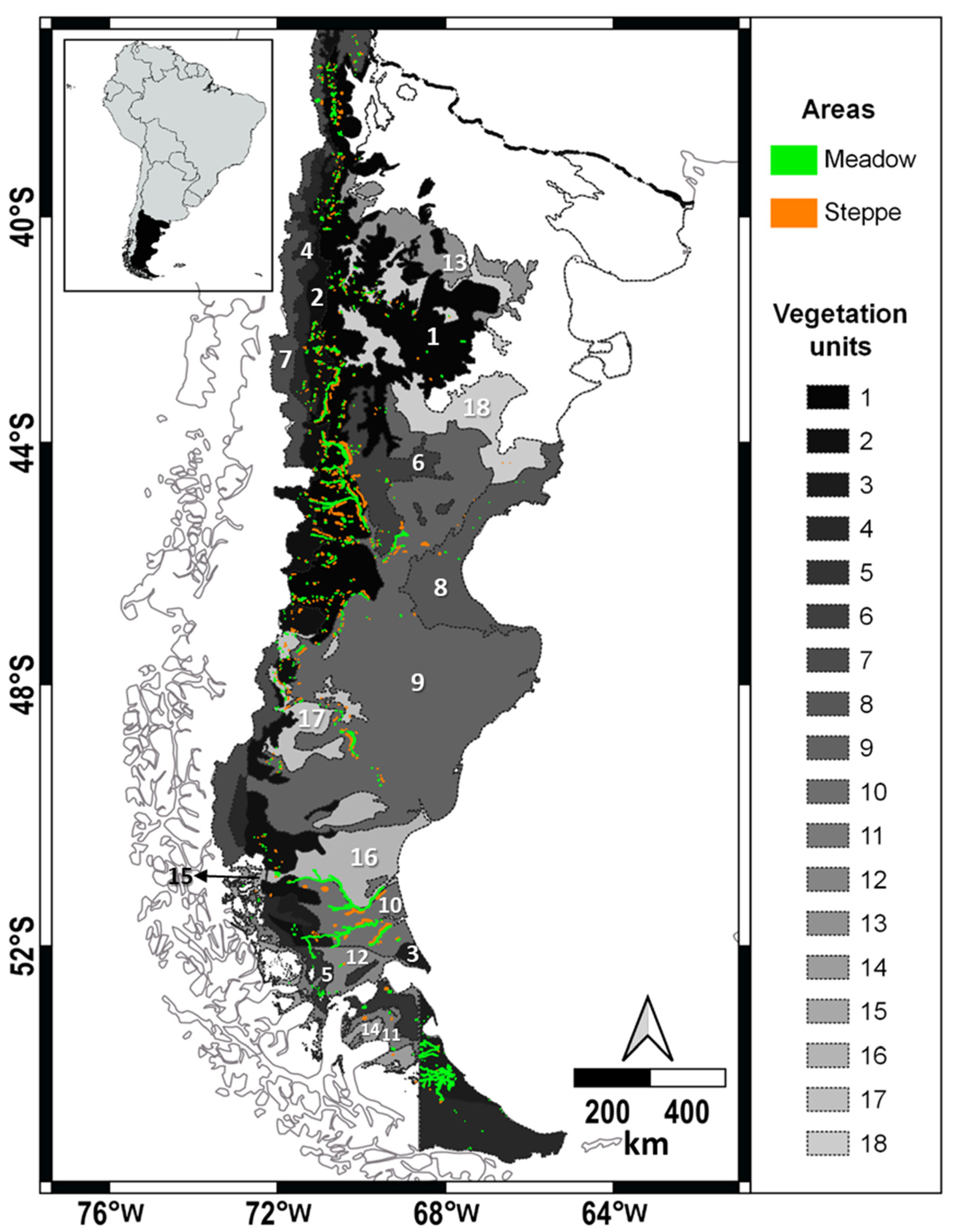
2.1. Study Area

The study area was circumscribed to the phytogeographic region of Patagonia, from the south of the Colorado River to the extreme south of the Tierra del Fuego Island (Figure 1). The climate of this wide region is cold temperate, with a mean annual temperature that oscillates between 12 °C in the north and 3 °C in the south, and absolute minimum temperatures below −20 °C [35]. Annual precipitation decreases and its variability increases from west to east [8,36]. On the western side of the Andes, the amount of annual rainfall exceeds 2000 mm [35]. In contrast, in the central part of extra-Andean Patagonia, annual precipitation reaches only 125 mm in the center east and 500 mm in the western part [36,37]. In most of the region, annual precipitation is concentrated in the winter period [25], with a consequent very marked summer water deficit [8]. However, the southern parts of the region is additionally affected by air masses coming from the Atlantic Ocean, which results in a more uniform seasonal distribution of precipitations [35] by manifesting some additional rains [8].

2.2. Data

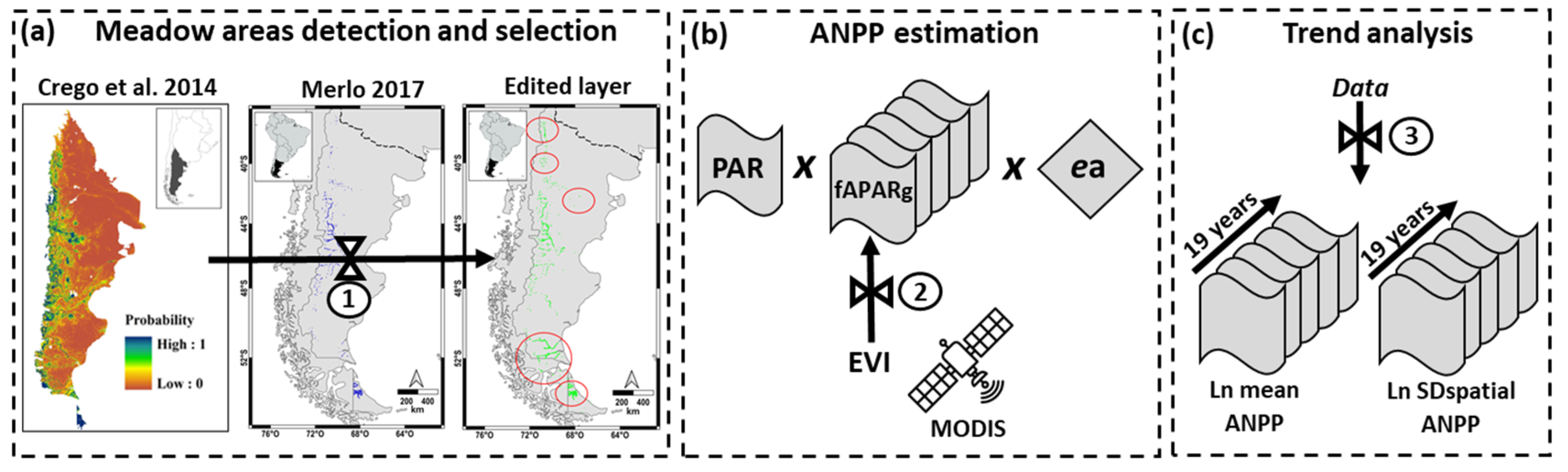
2.2.1. Meadow Area Detection and Selection

This study focused on selected meadow areas (Figure 2). These areas were obtained from a layer created by Merlo (2017) [40], based on Crego et al. (2014) [41]. In addition, we included areas not contained in Merlo (2017) and selected steppe areas adjacent to the selected meadows (Figure 1). The vector layer created by Merlo (2017) consisted of 150,000 ha of 450,000 ha of meadow areas selected from a classification carried out by Crego et al. (2014). This classification indicated the probability of containing more than 5% of meadow within a 100 ha pixel. Merlo (2017) selected only pixels with at least 80% probability of containing 5% or more meadow areas. However, given the coarse resolution of the pixel used in the classification, further analyses were needed. Specifically, we redrew some of the meadow area boundaries, leaving out areas that were not visually identified as meadows (Figure S1). This action was especially important for meadow areas located on Tierra del Fuego Island. In addition, we manually delimited new meadow areas (Figure S1) from meadows identified in the literature [6,42,43,44,45,46,47,48,49] but not classified by Crego et al. (2014). As a result of this edition, the layer consisted of 374,000 ha of meadows, distributed in 855 meadow polygons (Figure 2).
In addition, we generated a similar layer of steppe areas neighboring meadow areas (Figure 1). We drew polygons of selected steppe areas close to the meadow areas and of similar size. In some cases, it was not possible to delimit nearby steppe areas; this action was carried out across 65% of the meadow surface, accounting for 240,000 ha of steppe, represented by 739 steppe polygons.

2.2.2. ANPP Estimation

We estimated monthly ANPP for all the pixels contained in each meadow and neighboring steppe areas (Figure 2). For this, we used a specific software developed for monthly forage production estimations for grazing areas of South America [50]. This software is based on satellite information provided by the MODIS project, for a pixel size of 250 m per side, for the period of 2000–2019, with the exception of some areas located in the southern end of the region (involving areas in the MODIS scene h14v14 that were not yet available in the software). In these areas, the estimation was made using the Google Earth Engine platform (GEE) [51]. In all cases, we selected only those pixels with high-quality reliability (by the selection of pixels with 0 value of the MODIS band SummaryQA), and we estimated ANPP via the logic of a radiative model (Equation (1)) [52].
ANPP = PAR × fAPARg × ea
This model establishes that ANPP (in g m−2 day−1) is a consequence of the triple product between the incoming photosynthetically active radiation (PAR, in MJ m−2 day−1), the fraction of PAR which is absorbed (fAPARg, a proportion), and the radiation use efficiency for aboveground production (ea, in g dry matter MJ−1).
These components of the radiative model were obtained from different sources. PAR was obtained via digitizing maps describing the mean monthly dynamics of PAR across Patagonia [53]. fAPARg was estimated from information provided by remote sensing, through the Enhanced Vegetation Index (EVI). EVI values were obtained from the product MOD13Q1, every 16 days at a resolution of 5.3 ha from the year 2000 to 2019 (Figure 2). The transformation of EVI to fAPARg used the same parameters for meadows and steppes (fAPARg = 1.15 * EVI − 0.0174, for EVI values less than 0.0159 or greater than 0.8412 corresponded to 0 and 0.95 fAPARg, respectively) [50]. ea was equal to 0.72 g dry matter MJ−1 for meadows and 0.31 g dry matter MJ−1 for steppes [12,54]. This approximation does not consider seasonal variations of ea and assumes that the variations in potential inter-annual variations of ANPP are due to PAR and fAPARg, in seasonal terms for PAR, and seasonal and inter-annual terms for fAPARg. This assumption implies that seasonal variations in ea are absorbed over a longer period by fAPARg [55,56]. Spatially, ANPP estimations and their variations were a consequence of the spatial patterns of PAR, fAPARg, and ea, in this last one only when comparing meadow areas to the nearby steppes.

2.2.3. Geographic and Climatic Data

Each area, either meadow or steppe areas, was associated with its political district (department and province), phytogeographic unit [38,39], and climatic data (precipitation and temperature). We obtained temperature and precipitation records for the period 2000–2019 from monthly estimates at a 0.05° resolution generated by the TerraClimate dataset [57] and obtained from GEE platform [51]. The annual period considered for temperature and precipitation data was related to the growing season of the vegetation, which we considered from July of a calendar year to June of the following one [10,11,12]. Hence, we considered the annual temperature as the average of the monthly temperatures corresponding to the growing season. Previously, we estimated the monthly mean temperature by averaging the monthly maximum and minimum temperatures. Regarding precipitation, we considered the precipitation of each growing season as that registered from May of a calendar year to April of the following one, given that in most of Patagonia, rainfall accumulates in the autumn–winter period [36,37]. Thus, we then estimated mean annual temperature (MAT) and mean annual precipitation (MAP) for the 2000–2019 period.

2.2.4. Database Processing

From the monthly ANPP estimates for each MODIS pixel, we obtained a database with almost 13 million records for meadows (19 years * 12 months * 55,000 pixels, from 855 areas) and 8 million for steppes (19 years * 12 months * 36,000 pixels, from 739 areas, Figure 2). We discarded either meadow or steppe areas with excessive missing data related to pixel atmospheric quality. Therefore, we performed a series of analyses considering the pixels within each area and evaluated the amount of data per area to make the final decision. This analysis consisted of four steps. Firstly, we associated each monthly ANPP estimation per pixel with a specific growing season, from July of a calendar year to June of the following one. Secondly, we defined three phases, within the growing season: “resting” (May, June, July, and August), “intermediate” (March, April, September, and October), and “active” (January, February, November and December). This division followed previous studies describing the seasonal dynamics of ANPP or spectral indices for both meadows and steppes [10,11,12]. Thirdly, we discarded pixels that had 50% or more missing growing season data in the “active” phase. Lastly, we removed areas with less than 14 growing seasons and less than 50% of the pixels in it. In large areas (greater than 100 ha), we relaxed the previous condition to 12 seasons and more than 100 ha (20 pixels) with data. As a consequence of this processing, 738 polygons of meadow and 680 of steppe remained.
Once pixels and areas with excessive missing data were discarded, we built two indicators per area and growing season. First, the annual ANPP is estimated from the average of the annual ANPP of all the pixels contained in each area. Second, the ANPP heterogeneity, estimated from the spatial standard deviation (SDspatial) of the annual ANPP, is also calculated from the pixels contained in each area. Because of the described processing, we obtained a matrix where each row represented a meadow or steppe area (n = 738 and n = 680, respectively) for each of the 19 seasons (26,942 rows). Therefore, this matrix was composed of the annual ANPP, the SDspatial of it, and the climate descriptors, for each of the 19 growing seasons.
Finally, to avoid including meadow or steppe areas with possible errors in their delimitation and following previous similar procedures [12], we estimated the precipitation use efficiency (PUE) as the ratio between the mean annual ANPP and MAP. Those areas that were below or above the 5% and 95% percentiles, respectively, were discarded from the analyses. Thus, the final data frame included 665 meadow areas, which represented 250,000 ha, and 617 steppe areas, which represented 176,000 ha.

2.3. Analysis

To address the first objective and to analyze the trends of ANPP and its heterogeneity over time, we estimated the relative rate of change (RRC) of ANPP and its spatial standard deviation per meadow area. To estimate both RRCs for each area, we regressed either ln (ANPP) or ln (SDspatial of ANPP) against the independent variable time (19 years) [58]. The respective slopes represented a direct estimator of the relative annual change of ANPP and its heterogeneity. Then, we took three complementary approaches.
The first approach aimed to estimate the trend of the entire meadow and steppe ecosystems. Consequently, we estimated the mean annual ANPP weighted by the area, in meadows and steppes, and for each of the 19 seasons. Furthermore, we divided the analysis into two more groups. First, we analyzed the changes for the entire type of ecosystem, meadow or steppe. Second, we looked at the areas within each type of ecosystem by type of trend, positive or negative. This analysis allowed us to understand the relative importance of the size of each meadow area on the overall trend of the ecosystem. In the case of steppes, the analysis did not aim to characterize the importance by weighted area but represents a reference for understanding the behavior of vegetation in sync with climate variations. Then, to evaluate the average ANPP trends, we described using simple linear regression models the association between the weighted ANPP, total, and for each subset, with season.
For the second approach, we compared the RRC of ANPP by pair of meadow and steppe areas to corroborate if the observed patterns were similar across the two types of vegetation. We evaluated the association between the RRC of ANPP in meadows compared to that of the nearby steppe areas through the Pearson regression coefficient (“psych” R package [59]). Furthermore, we counted the pairs, meadow and nearby steppe by type of RRC of ANPP, where there were four potential scenarios, both negative, both positive, and either positive or negative.
For the third and last approach, we evaluated the association between the trends of ANPP and its heterogeneity with environmental controls across the regional gradient in three steps. First, to understand if meadow areas inserted in the arid end of the region had a steeper change of ANPP and heterogeneity over time, we examined the association between the RRC of ANPP and its heterogeneity with MAP and MAT. Second, to understand if trends of ANPP and its heterogeneity were associated with changes over time in precipitation and temperature, we also examined the association between the RRC of ANPP and its heterogeneity with the RRC of MAP and MAT, both in meadow and steppe areas. The RRC of MAP and MAT were estimated for each meadow and steppe area using the same procedure described for the RRC of the ANPP. In these first two steps, we performed multiple linear regression models, which considered the type of vegetation (meadow or steppe) as an independent categorical variable and evaluated each independent variable separately, that is, the MAP, MAT, and RRC of MAP and MAT. Third, we performed two multiple regressions to identify which independent variable (standardized MAP and MAT versus their RRC) had the greatest influence on each response variable (RRC of the ANPP and its heterogeneity). In both regressions, the type of vegetation was also considered an independent categorical variable.
To address the second objective, we evaluated the impact on the livestock carrying capacity of meadows in the region and estimated the initial and final mean livestock carrying capacity for the 2000–2019 period. We estimated the carrying capacity for each meadow area based on ANPP, since it is the main variable that determines it, using the Equations (2) and (3) proposed by Golluscio et al. (1998), which are expressed as follows:
Carrying capacity (sheep ha−1) = (ANPP ∗ HI/100)/individual consumption,
HI (%) = −5.71 + 0.7154 ∗ (ANPP)0.5,
where HI represents the harvest index, the proportion of ANPP that can be potentially consumed by sheep. We assumed an annual individual consumption of 350 kg dry matter sheep−1 yr−1, considering a 40 kg sheep with a daily intake of 2.4% of its body weight [60]. To estimate the initial HI and carrying capacity values, we considered the ANPP of the first season 2000–2001 in kg dry matter ha−1 yr−1. Instead, to estimate the final HI and carrying capacity, we considered the final ANPP as follows:
ANPPfinal = ANPPinitial ∗ (1 + RRC)18,
where RRC represents the relative rate of change expressed in yr−1, and 18 represents the final growing season used in the analysis. These estimations per meadow area were also assigned to four potential trend syndromes (described below, related to the third specific objective). We carried out two types of ANOVA and Tukey’s test, on the one hand, to determine if the degradation trends had different carrying capacity values and, on the other, to quantify the net effect of the potential trends of ANPP on the most extended activity in the area: direct grazing by sheep. In the first test, the response variables were the estimations of the initial and final carrying capacity by area, and the independent variable was the trend syndrome, which had four levels (I, II, III, and IV). The second test compared the overall change in the carrying capacity of meadows, where the independent variable was the moment, which had two levels (initial and final).
To address the third and final specific objective and to propose and evaluate the degradation trends of these ecosystems, based on four different trend syndromes derived from the combination of temporal trends of the ANPP and its heterogeneity, we evaluated the percentage of meadow areas in four possible quadrants, which represented the proposed trend syndromes (Figure 3). Regardless of statistical significance, the upper left quadrant (I) corresponded to cases in which the RRC of the ANPP was positive, but that of its heterogeneity was negative, representing an improvement situation; the upper right quadrant (II) corresponded to cases in which both RRCs were positive, representing slight degradation; the lower right one (III) to cases in which the RRC of the ANPP was negative, but that of its heterogeneity was positive, representing moderate degradation; and the lower left (IV) to cases in which both RRCs were negative, representing severe degradation. In turn, we quantified the area represented by each of these possible trend syndromes, both for the total and for each phytogeographic unit of Patagonia.
All processes were conducted using R software (version 4.0.2, R Core Team 2020), where for data manipulation, we used “dplyr” [61] and “tidyr” [62] packages and Microsoft Excel.

3. Results

3.1. ANPP Trends

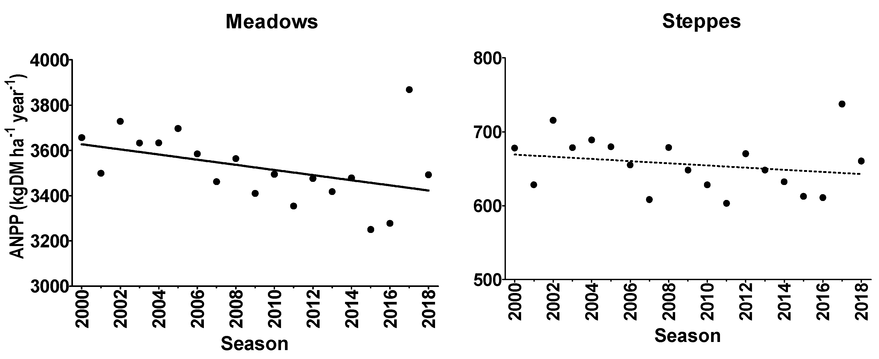
3.1.1. Average ANPP Trends

In the last two decades, the area-weighted mean ANPP of Patagonian meadows decreased by 6%, from an average of 3600 kg/ha.yr−1 to 3400 kg/ha.yr−1 (11.4 kg dry matter ha−1 per season, Figure 4 left panel). On the contrary, the neighboring steppe areas did not show a significant trend (Figure 4 right panel). However, if only meadow areas with a negative trend are considered, ANPP decreased by 11% from 3800 to 3400 kg/ha.yr−1, at a decrease rate of 21.4 kg dry matter ha−1 per season (ANPP = 46,636.72 − 21.43 * season, p value = 0.004, R2 = 0.39). In contrast, in meadow areas with a positive trend, ANPP increased by 8%, from 3200 to 3500 kg/ha.yr−1, at an average positive rate of 16.1 kg dry matter ha−1 per season (ANPP = −28,887.84 + 16.06 * season, p value = 0.01, R2 = 0.32). Additionally, meadow areas with a negative trend presented higher ANPP values at the beginning of the studied period compared to those areas with a positive trend. However, at the end of the analyzed period, the ANPP of both types was similar.

3.1.2. Relative Rate of Change of ANPP by Pair of Meadow and Steppe Areas

The ANPP relative rate of change (RRC) of meadow areas was positively associated with that of the neighboring steppes (Pearson’s coefficient = 0.39, p value < 0.05), and, independent of the sign, the RRC was more variable in meadows than in steppes (Figure 5). ANPP RRC of meadow areas had a similar sign (either positive or negative) to that of the nearby steppe ones in 66% of the cases (Figure 5). In 42% of the analyzed pairs, both had a negative trend of ANPP. Within this pattern, in 85% of the cases, the relative decrease in ANPP was greater in meadows than in steppes. In 24% of the analyzed pairs, both had a positive trend (Figure 5). Within this pattern, in 79% of the cases, the relative increase in ANPP was greater in meadows than in steppes. When looking at opposite trends, the one that dominated was that where the RRC was negative in meadows but positive in steppes, with 21% of the cases. The other combination of opposite trends, where meadow areas had a positive RRC, but the nearby steppe negative represented 13% of the cases (Figure 5). The RRC of the ANPP in meadows varied between −0.036 and 0.022 year−1, while, in steppes, it varied between −0.011 and 0.026 year−1 (Figure 5). In other words, the changes in meadows implied an annual decrease in the ANPP of 3.6% and an increase of 2.2%, while in steppes, they were 1.1% and 2.6%, respectively.

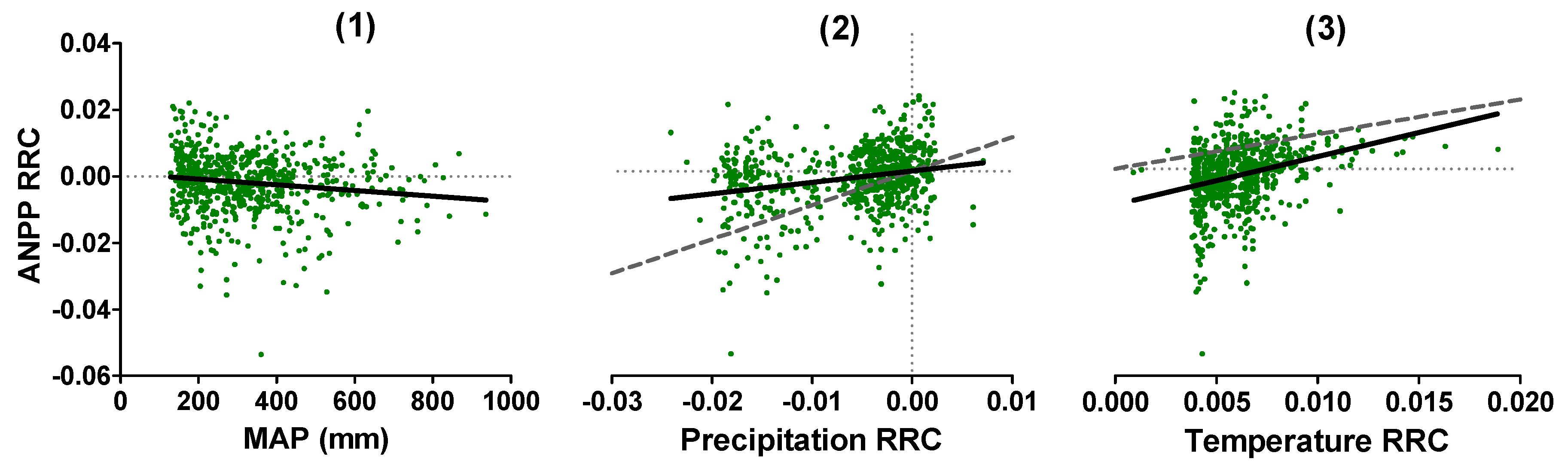
3.1.3. ANPP Trends Relationship with Environmental Controls

The variables considered related to environmental controls did not explain the variation in the RRC of ANPP and its heterogeneity between meadow or steppe areas since the proportion of the variability explained by the evaluated models was very low (Figure S2, Table S1). Nevertheless, ANPP RRC was more variable in the arid end of the MAP gradient than in the humid one (Figure 6(1)). For example, below 400 mm of MAP, ANPP RRC ranged from −0.0536 to 0.0220 but from −0.0198 to 0.0196 for sites above 600 mm of MAP. Furthermore, precipitation had a predominance of negative trends, while temperature only had positive ones (Figure 6(2,3) and Figure S3). Additionally, despite the low fit, meadow areas ANPP RRC was negatively associated with mean annual precipitation (p value < 0.001, R2 = 0.03, Figure 6(1), Table S1), while no statistical pattern was observed for the nearby steppe areas (Figure S2, Table S1). Independently of the MAP, ANPP RRC was positively associated with RRC of precipitation (p value < 0.001, R2 = 0.06, Figure 6(2)) and temperature (p value < 0.001, R2 = 0.09, Figure 6(3)) when considered in a multiple regression approach (Table S1).

3.2. Impact on Livestock Carrying Capacity of Meadows

From 2000 to 2019, the carrying capacity changed in two of the four proposed trend syndromes (Figure 7, blue lowercase letters). It increased by 19%, from 2.7 to 3.2 sheep ha1, in meadows under Syndrome II (positive ANPP and SDspatial RRC) and decreased in a similar proportion, from 5.1 to 4.3 sheep ha1, in those under Syndrome III (negative ANPP and positive SDspatial RRC), while there was no significant change in meadows under Trend Syndromes I (positive ANPP and negative SDspatial RRC) and IV (negative ANPP and SDspatial RRC) (Figure 7, blue lowercase letters). In addition, although the initial mean carrying capacity was higher in meadows under Trend Syndromes III and IV (Figure 7, black capital letters), the final mean carrying capacity of the latter did not differ from that under Trend Syndromes I and II (Figure 7, black lowercase letters). Due to the fact that Trend Syndromes III and IV represented 75% of the evaluated area, the total amount of animals decreased by 75,000 sheep in the entire region (Figure 7, Total) or 8%.

3.3. Trend Syndromes in Meadow Areas

Meadow areas’ ANPP RRC was positively associated with ANPP SDspatial RRC (p value < 0.0001, Pearson coefficient = 0.55). Most meadow areas (41%) presented a trend syndrome of severe degradation, in which RRCs were negative, representing 55% of the studied area (~137,000 ha) (Figure 8(1), Quadrant IV). The second most important (27%) trend syndrome was slight degradation, in which both RRCs were positive, and it represented 19% of the studied area (~47,000 ha) (Figure 8(1), Quadrant II,). The third most important (16%) was moderate degradation, in which ANPP RRC was negative, but its SDspatial had a positive RRC, and it represented 20% of the studied area (~47,000 ha) (Figure 8(1), Quadrant III). Finally, a few meadow areas (16%) presented an improvement situation, in which ANPP increased and its SDspatial decreased over time, and it represented only 7% of the studied area (~16,000 ha) (Figure 8(1), Quadrant I). Moreover, the Trend Syndromes IV, II, and III were distributed in almost all the phytogeographic units containing meadow areas (Figure 8(2)), although around 77% of the area of meadows that presented each of these trend syndromes were only in three phytogeographic units (Figure 8(3)). Instead, Syndrome I was distributed in fewer units, one, two, and nine (Figure 8(3)), representing 94% of the cases.

4. Discussion

Overall, our results highlighted three main aspects. First, ANPP decreased over time in most of the studied meadow areas, suggesting meadow desertification, but in a few ones, ANPP increased. These temporal trends, characterized by the relative rate of change, were greater in meadows than in steppes. Additionally, the RRC of ANPP was more variable towards the arid end of the analyzed moisture gradient. Second, the observed patterns suggest a net decrease over time in the provision of two key ecosystem services, its potential capacity as a carbon input and the provision of forage for livestock. Third, our approach indicated that 55% of the analyzed meadow areas corresponded to a severe degradation trend, where both ANPP and its spatial variation decreased from 2000 to 2019. If the following degradation trend syndrome is considered, where ANPP decreased over time, but its spatial variation increased, it reached 75% of the analyzed areas. Otherwise, the remaining 25% experienced an increase in ANPP over time.
The ANPP of meadows decreased in the first two decades of the 2000s, while the nearby steppes had, in many cases, lower and opposite trends, or no trend at all. In correspondence with these trends in the steppes, previous studies determined losses of vegetation cover in the steppes in the period 2008–2012 [8] and increases in 2014–2019 [63]. Furthermore, meadow areas’ ANPP trends suggest an effect of desertification mediated not only by environmental factors, but management related as well. Regarding the environmental role, and when comparing the RRC between meadows from the nearby steppes, it supports the proposed mechanism, which indicated that soils from the surrounding steppe areas exhibited a maximum water-holding capacity lower than the mean annual precipitation [24,25], leading to the lower magnitude of ANPP RRC compared to that of meadow areas. This suggests that the accumulated water in lower portions of the landscape during winter, where meadows are located, had an impact over time in meadows. However, when comparing the ANPP RRC between meadow areas of Patagonia with that of grasslands in the nearby Pampas biome, with similar ANPP ranges but independent of water table regimes, the latter had up to three times greater RRC [58]. Thus, the influence of the water table in meadows acts as a buffer against events of drought or intense heat in comparison to other similarly productive grasslands.
Regarding the human-related factors, at least two observed patterns emphasized its role. Firstly, and more notoriously, there were meadow areas with opposite ANPP trend to the nearby steppe areas trend and that of precipitation as well. Secondly, the environmental factors explained very little of the variation in the ANPP trend. Moreover, in many cases where the sign of the ANPP trend was like that of precipitation, the former had a higher magnitude, suggesting changes not only mediated by the evaluated environmental factor. Meadow areas with negative ANPP trends and opposite to other factors, or higher than that of precipitation, suggests overgrazing [64] since it is the main human-related activity across the region. Within the analyzed period, domestic and wild herbivore stocking increased, mainly through livestock and guanacos (the main wild herbivore), beyond the region carrying capacity [28]. Potentially, meadow areas might have been the rangeland areas that hosted livestock numbers, given the limitation steppe vegetation imposes on forage availability, quality, and livestock bite size [65]. On the contrary, positive trends suggest the implementation of practices associated with water redistribution [29] or fertilization [23].
ANPP’s negative trend impacted two ecosystem services: carbon (C) dynamics and livestock carrying capacity. In the last two decades, assuming a 45% C concentration in the dry matter [66], ANPP’s negative trend represented a total decrease in C inputs of 24,220 megagrams (Mg). Enriquez et al. (2015) [64], working across a series of meadows in Patagonia, determined that long-term overgrazing altered the C cycle by reducing on average 2900 kgDM ha−1 (30%) and 6700 kgDM ha−1 (65%) of above and belowground plant biomass, respectively, and decreasing C inputs to the soil, which meant a decrease of 35% of the total ecosystem C pool. Regarding the second ecosystem service (the carrying capacity), ANPP´s negative trend represented an 8% decrease. In sync with our findings, from 2002 to 2018, sheep decreased by 2.2 million across 69 million ha of Patagonia [67,68]. Given the observed stocking numbers decreased and the meadow’s carrying capacity reduction, these systems potentially accounted for 3.3% (73,000 sheep) of the variation, representing less than 0.5% of the area. Additionally, other factors beyond ANPP may have affected negatively the stocking numbers of Patagonia, including reductions in drinking water points and/or forage quality [8].
The proposed trend syndromes classification provides new insights into one of the iconic areas associated with the study of desertification, Patagonia [69]. The quantification and determination of desertification require reference situations to be compared and/or long-term ANPP datasets [70,71]. The proposed approach sorted both limitations using nearby steppe areas as references and a metric related to ANPP but independent of the mean itself (i.e., the relative rate of change). We believe this approach complements previous metrics relating to ANPP and precipitation dynamics, as are the precipitation use efficiency and the marginal response to precipitation [69], which are of less use in this type of ecosystem. Through this approach, we were able to indicate that 55% (~137,000 ha) of the evaluated area is under the worst syndrome of degradation. Across Patagonia, considering a similar period of time, NDVI inter-annual dynamics were majorly associated with the description of a negative trend, which recently shifted to a positive phase [72]. Different from that description, meadow areas seem to be under a long-term negative trend exacerbated by a reduction in ANPP’s spatial variation. Furthermore, the negative trend of both ANPP’s mean and its spatial variation suggests the shift towards a new stable state [73]. This new state suggests the loss of soil layers, specifically the ones rich in soil organic matter [64,74]. If this new stable state is confirmed, it would indicate that reversing this trend will require probably a longer period, driven by soil formation processes [75].

5. Conclusions

Overall, we were able to quantify, for the first time, the degradation trends in meadows along a wide environmental gradient, as anticipated by different local conceptual models [30,31,32,76,77]. In the last two decades, for the set of studied meadows, the ANPP decreased, which reduced their livestock carrying capacity, while the nearby steppes remained relatively stable. In this sense, the trend syndrome that prevailed across meadow areas was the one that represented the worst syndrome of degradation. Therefore, it is essential to adopt management practices that allow sustainable use of this key ecosystem. These results could help identify priority areas along with specific management decisions given the different trend syndromes. Moreover, through the characterization of these syndromes, future studies could evaluate the impact of different management practices applied in meadows and encourage the development on a larger scale of those that present improvement situations.
Furthermore, our findings are essential to establish new meadow areas to protect and complement previous studies that prioritized their conservation based on aquatic and terrestrial biodiversity [78]. In this sense, future efforts should lead to an inventory of meadows, that allows knowing their location with greater precision and accuracy, and a vegetation and soil monitoring network, similar to the one existing in steppe areas [79], both combined with the power of remote sensing. Thus, our results could be taken as a basis, in combination with a recent distribution map of wetlands of Argentina [14], to inventory them and install monitoring stations, which implies a great challenge given the large territorial extension in which the meadows are located.

Supplementary Materials

The following supporting information can be downloaded at: https://www.mdpi.com/article/10.3390/rs15102531/s1. Figure S1. Comparison between the layer of meadow areas created by Merlo (2017; yellow polygons) [40], based on a previous classification carried out by Crego et al. (2014) [41], and the layer resulting from our edition (green polygons). Differences between both layers in Patagonia (Panel 1) are exemplified in the Argentine province of Santa Cruz (Panel 2, a), showing the incorporation of new meadow areas based on the literature, and Tierra del Fuego (Panel 2, b.1 and b.2) and showing the contrast between both layers. Boxes with dotted lines correspond to areas represented in greater detail, on a smaller scale. The dashed black line in Panel 1 corresponds to the Colorado River. Figure S2. Relative rate of change (RRC) of aboveground net primary productivity (ANPP) (a) and RRC of the spatial standard deviation of the ANPP (b) as a function of (1) mean annual precipitation (MAP), (2) mean annual temperature (MAT), (3) precipitation RRC, and (4) temperature RRC, in meadows (green dots) and steppes (orange dots). Each point corresponds to an area of meadow or steppe evaluated, for the period between 2000 and 2019. The black lines represent the fit of a statistically significant linear model (p value < 0.05) for meadows or both (a thin dashed line means no difference between their slopes). For more details on the models represented in this figure, see Table S1. Panels a.1, a.3, and a.4 are the same ones represented in Figure 5. Figure S3. Box plot of the relative rate of change (RRC) of the precipitation and temperature registered in meadow and steppe areas for the period 2000–2019. Table S1. Multiple regression models of (a) the relative rate of change (RRC) of the mean annual aboveground net primary productivity (ANPP) and (b) the RRC of the spatial standard deviation (SD) of the ANPP, depending on the type of vegetation (TVeg, either meadow or steppe), of the environmental controls, mean annual precipitation (MAP), mean annual temperature (MAT), and their respective RRC (RRCMAP and RRCMAT). The first column indicates the three types of models evaluated, from which it is represented the association of said dependent variables (a and b) with the TVeg and (1) the MAP, (2) the MAT, (3) both standardized environmental controls (MAP_st and MAT_st), (4) the RRCMAP, (5) the RRCMAT, and (6) with both RRC (RRCMAP and RRCMAT). Models (1), (2), (4), and (5) are represented graphically in Figure S2. For each dependent variable included in the models, the estimators, the standard error, the p value, and the adjusted R2 are informed. The intercept refers to steppe areas with no effect on the independent variables. Significant effects (p value < 0.05) are indicated in bold.

Author Contributions

Conceptualization and methodology, M.C., G.I., G.G.M. and M.O.; formal analysis, M.C. and G.I.; data curation, M.C.; writing—original draft preparation, M.C. and G.I.; writing—review and editing, M.C., G.I., G.G.M. and M.O. All authors have read and agreed to the published version of the manuscript.

Funding

This study was carried out with the funding of the Consejo Nacional de Investigaciones Científicas y Técnicas (CONICET) and the Instituto Nacional de Tecnología Agropecuaria (INTA).

Data Availability Statement

Not applicable.

Conflicts of Interest

The authors declare no conflict of interest.

References

  1. Xiaoyan, B.; Suocheng, D.; Wenbao, M.; Fujia, L. Spatial-temporal change of carbon storage and sink of wetland ecosystem in arid regions, Ningxia Plain. Atmos. Environ. 2019, 204, 89–101. [Google Scholar] [CrossRef]
  2. Fang, Q.; Wang, G.; Liu, T.; Xue, B.L.; Yinglan, A. Controls of carbon flux in a semi-arid grassland ecosystem experiencing wetland loss: Vegetation patterns and environmental variables. Agric. For. Meteorol. 2018, 259, 196–210. [Google Scholar] [CrossRef]
  3. UNCCD. Elaboration of an International Convention to Combat Desertification in Countries Experiencing Serious Drought and/or Desertification, Particularly in Africa. 1994, Volume 24, pp. 1–58. Available online: https://wedocs.unep.org/handle/20.500.11822/27569;jsessionid=3C6D21F808FF14535A97268CAD716845 (accessed on 7 May 2023).
  4. Fluet-Chouinard, E.; Stocker, B.D.; Zhang, Z.; Malhotra, A.; Melton, J.R.; Poulter, B.; Kaplan, J.O.; Goldewijk, K.K.; Siebert, S.; Minayeva, T.; et al. Extensive global wetland loss over the past three centuries. Nature 2023, 614, 281–286. [Google Scholar] [CrossRef] [PubMed]
  5. Brinson, M.M.; Malvárez, A.I. Temperate freshwater wetlands: Types, status, and threats. Environ. Conserv. 2002, 29, 115–133. [Google Scholar] [CrossRef]
  6. Mazzoni, E.; Rabassa, J. Types and internal hydro-geomorphologic variability of mallines (wet-meadows) of Patagonia: Emphasis on volcanic plateaus. J. S. Am. Earth Sci. 2013, 46, 170–182. [Google Scholar] [CrossRef]
  7. Collantes, M.B.; Anchorena, J.; Stoffella, S.; Escartín, C.; Rauber, R. Wetlands of the magellanic steppe (Tierra del Fuego, Argentina). Folia Geobot. 2009, 44, 227–245. [Google Scholar] [CrossRef]
  8. Oliva, G.; García, G.; Ferrante, D.; Massara, V.; Rimoldi, P.; Díaz, B.; Paredes, P. Estado de los Recursos Naturales de la Patagonia Sur Centro Regional Patagonia; Instituto Nacional de Tecnología Agropecuaria: EEA Santa Cruz, Argentina, 2017. [Google Scholar] [CrossRef]
  9. Chimner, R.a.; Bonvissuto, G.L.; Cremona, M.V.; Gaitan, J.J.; Lopez, C.R. Ecohydrological conditions of wetlands along a precipitation gradient in Patagonia, Argentina. Ecol. Austral 2011, 21, 329–337. [Google Scholar]
  10. Paruelo, J.M.; Golluscio, R.A.; Guerschman, J.P.; Cesa, A.; Jouve, V.V.; Garbulsky, M.F. Regional scale relationships between ecosystem structure and functioning: The case of the Patagonian steppes. Glob. Ecol. Biogeogr. 2004, 13, 385–395. [Google Scholar] [CrossRef]
  11. Buono, G.; Oesterheld, M.; Nakamatsu, V.; Paruelo, J.M. Spatial and temporal variation of primary production of Patagonian wet meadows. J. Arid Environ. 2010, 74, 1257–1261. [Google Scholar] [CrossRef]
  12. Irisarri, J.G.N.; Oesterheld, M.; Paruelo, J.M.; Texeira, M.A. Patterns and controls of above-ground net primary production in meadows of Patagonia. A remote sensing approach. J. Veg. Sci. 2012, 23, 114–126. [Google Scholar] [CrossRef]
  13. Raffaele, E. Susceptibility of a Patagonian mallín flooded meadow to invasion by exotic species. Biol. Invasions 2004, 6, 473–481. [Google Scholar] [CrossRef]
  14. Navarro, M.; Navarro, C.; Barrios, R.; Calamari, N.; Dieta, V.; Martínez García, G.; Iturralde Elortegui, M.; Kurtz, D.; Michard, N.; Paredes, P.; et al. Mapa de Distribución Potencial de Humedales en Argentina. Informe Técnico. 2022. Available online: https://intahumedales.users.earthengine.app/view/mapahumedalesargentina (accessed on 20 April 2023).
  15. Bonvissuto, G.; Somlo, R.; Ayesa, J.; Lanciotti, M.L.; Moricz de Tecso, E. La condición de los mallines del área ecológica sierras y mesetas de Patagonia. Rev. Argentina Prod. Anim. 1992, 12, 391–400. [Google Scholar]
  16. Bruce, A.; Dufilho, A.C. Los mallines en Patagonia: Una perspectiva histórico cultural de los recursos naturales. Mundo Agrar. 2002, 2. Available online: http://www.scielo.org.ar/scielo.php?pid=S1515-59942002000100005&script=sci_arttext&tlng=en (accessed on 7 May 2023).
  17. Collantes, M.B.; Faggi, A.M. Los Humedales del Sur de Sudamérica. Tópicos Sobre Humedales Subtropicales y Templados de Sudamérica; Unesco: Montevideo, Uruguay, 1999. [Google Scholar]
  18. Easdale, M.; Gaitan, J. Relación entre la superficie y clase de mallines y la composición de la estructura ganadera en establecimientos del noroeste de la Patagonia. Rev. Argent. Prod. Anim. 2010, 30, 69–80. [Google Scholar]
  19. Golluscio, R.A.; Deregibus, V.A.; Paruelo, J.M. Sustainability and range management in the Patagonian steppes. Ecol. Austral 1998, 8, 265–284. [Google Scholar]
  20. Irisarri, J.G.N.; Texeira, M.; Oesterheld, M.; Verón, S.R.; Della Nave, F.; Paruelo, J.M. Discriminating the biophysical signal from human-induced effects on long-term primary production dynamics. The case of Patagonia. Glob. Chang. Biol. 2021, 27, 4381–4391. [Google Scholar] [CrossRef] [PubMed]
  21. Oliva, G.; Gaitan, J.; Ferrante, D. Humans Cause Deserts: Evidence of Irreversible Changes in Argentinian Patagonia Rangelands. In The End of Desertification? Springer: Berlin/Heidelberg, Germany, 2016; pp. 363–386. [Google Scholar] [CrossRef]
  22. Zhao, M.; Running, S.W. Drought-induced reduction in global terrestrial net primary production from 2000 through 2009. Science 2010, 329, 940–943. [Google Scholar] [CrossRef]
  23. García Martínez, G.C.; Ciari, G.; Gaitan, J.; Caruso, C.; Nagahama, N.; Opazo, W.; Nakamatsu, V.; Lloyd, C.; Cotut, C.; Irisarri, J.G.N.; et al. Diagnóstico de la evolución del clima y los pastizales naturales en el noroeste de la provincia de Chubut en el período 2000-2014. Agri. Sci. 2017, 34, 59–69. [Google Scholar]
  24. Paruelo, J.M.; Sala, O.E. Water Losses in the Patagonian Steppe: A Modelling Approach. Ecology 1995, 76, 510–520. [Google Scholar] [CrossRef]
  25. Bandieri, L.M.; Fernández, R.J.; Bisigato, A.J. Risks of Neglecting Phenology When Assessing Climatic Controls of Primary Production. Ecosystems 2020, 23, 164–174. [Google Scholar] [CrossRef]
  26. Spinoni, J.; Barbosa, P.; De Jager, A.; McCormick, N.; Naumann, G.; Vogt, J.V.; Magni, D.; Masante, D.; Mazzeschi, M. A new global database of meteorological drought events from 1951 to 2016. J. Hydrol. Reg. Stud. 2019, 22, 100593. [Google Scholar] [CrossRef]
  27. Irisarri, J.G.N.; Cipriotti, P.A.; Texeira, M.; Curcio, M.H. Trends in ANPP Response to Temperature in Wetland Meadows across a Subcontinental Gradient in Patagonia. Meteorology 2022, 2, 15. [Google Scholar] [CrossRef]
  28. Oliva, G.; Paredes, P.; Ferrante, D.; Cepeda, C.; Rabinovich, J. Remotely sensed primary productivity shows that domestic and native herbivores combined are overgrazing Patagonia. J. Appl. Ecol. 2019, 56, 13408. [Google Scholar] [CrossRef]
  29. Boggio, F.; Cremona, M.V.; Aramayo, M.V.D.L.; Girardin, L.; Raffo, F.; Fariña, C.M.; Enriquez, A.S. Guía para el curso: “Restauración y Mejoramiento de Mallines Mediante obras de Redistribución del agua de Escurrimiento” Ediciones INTA 2019. Available online: http://hdl.handle.net/20.500.12123/6529 (accessed on 20 April 2023).
  30. Gandullo, R.; Schmid, P.; Peña, O. Dinámica de la vegetación de los humedales del Parque Nacional Laguna Blanca (Neuquén, Argentina). Propuesta de un modelo de estados y transiciones. Rev. Fac. Agron. UNLPam 2011, 20, 43–62. [Google Scholar]
  31. Aguiar, M.; Paruelo, J. Impacto humano sobre los ecosistemas: El caso de la desertificación. Cienchoy 2003, 13, 48–59. [Google Scholar]
  32. Collantes, M.B.; Escartín, C.; Braun, K.; Cingolani, A.; Anchorena, J. Grazing and grazing exclusion along a resource gradient in magellanic meadows of tierra del fuego. Rangel. Ecol. Manag. 2013, 66, 688–699. [Google Scholar] [CrossRef]
  33. Scheffer, M.; Bascompte, J.; Brock, W.A.; Brovkin, V.; Carpenter, S.R.; Dakos, V.; Held, H.; Van Nes, E.H.; Rietkerk, M.; Sugihara, G. Early-warning signals for critical transitions. Nature 2009, 461, 53–59. [Google Scholar] [CrossRef]
  34. Scheffer, M. Foreseeing tipping points. Nature 2010, 467, 411–412. [Google Scholar] [CrossRef]
  35. Paruelo, J.M.; Beltrán, A.; Jobbágy, E.G.; Sala, O.E.; Golluscio, R.A. The climate of Patagonia: General patterns and controls on biotic processes. Ecol. Austral 1998, 8, 85–102. [Google Scholar]
  36. Jobbágy, E.; Paruelo, J.M.; León, R.J.C. Estimación del régimen de precipitación a partir de la distancia a la cordillera en el noroeste de la Patagonia. Ecol. Austral 1995, 5, 47–53. [Google Scholar]
  37. León, R.J.C.; Bran, D.; Collantes, M.; Paruelo, J.M.; Soriano, A. Grandes unidades de vegetacion de la Patagonia extra andina. Ecol. Austral 1998, 8, 125–144. [Google Scholar]
  38. Oyarzabal, M.; Clavijo, J.; Oakley, L.; Biganzoli, F.; Tognetti, P.; Barberis, I.; Maturo, H.M.; Aragón, R.; Campanello, P.I.; Prado, D.; et al. Unidades de vegetación de la Argentina. Ecol. Austral 2018, 28, 040–063. [Google Scholar] [CrossRef]
  39. IDE Chile. Pisos Vegetacionales de Luebert y Pliscoff. Available online: https://www.ide.cl/index.php/flora-y-fauna/item/1524-pisos-vegetacionales-luebert-pliscoff-2017 (accessed on 9 February 2023).
  40. Merlo, L.R. Variación Espacial y Temporal de la Producción Primaria Neta Aérea de Mallines de la Patagonia. Master’s Thesis, Universidad de Buenos Aires, Facultad de Agronomía, Buenos Aires, Argentina, 2017. [Google Scholar]
  41. Crego, R.D.; Didier, K.A.; Nielsen, C.K. Modeling meadow distribution for conservation action in arid and semi-arid Patagonia, Argentina. J. Arid Environ. 2014, 102, 68–75. [Google Scholar] [CrossRef]
  42. Mazzoni, E.; Vázquez, M. Evaluación de pastizales húmedos para un aprovechamiento sustentable en la cuenca del río Gallegos (Provincia de Santa Cruz, Argentina). In Proceedings of the VIII Encuentro Latinoam, Geógrafos, Santiago, Chile, 4–10 March 2001; pp. 175–182. [Google Scholar]
  43. Lopez, C.R.; Gaitan, J.J.; Siffredi, G.L.; Ayesa, J.a; Lagorio, P. a Desarrollo de un sistema de informacion geografico (SIG) como herramienta para la planificacion manejo del pasroreo en mallines del Dpto. de Pilcaniyeu, Rio Negro. Revisita Cient. Agropecu. 2005, 9, 163–171. [Google Scholar]
  44. Utrilla, V.; Ferrante, D.; Peri, P.; Kofalt, J.C.; Humano, G. Efecto de la dinámica hídrica edáfica y ambiental sobre la productividad y calidad forrajera de mallines en la Patagonia Austral. Informe técnico final. EEA INTA Santa Cruz 2008, 31. [Google Scholar]
  45. Filipová, L.; Hédl, R.; Dančák, M. Magellanic Wetlands: More than Moor. Folia Geobot. 2013, 48, 163–188. [Google Scholar] [CrossRef]
  46. Utrilla, V. Monitoreo de indicadores de degradación en mallines bajo pastoreo ovino en el Sur de Santa Cruz. Mayéutica 2014, 40, 31. [Google Scholar] [CrossRef]
  47. Vargas, P.P.; Mazzoni, E. Caracterización de la Composición Florística y Productividad Primaria del Mallín Pali Aike, Patagonia Austral Argentina. 2014. Available online: https://redargentinadegeografiafisica.files.wordpress.com/2014/04/trabajo-vargas-y-mazzoni.pdf (accessed on 10 March 2023).
  48. Grima, D.; Vazquez, M.; Diez, P.; Investigadores, D.; Austral, P.; Acad, U.; Laboratorio, G. Composición Florística De Pequeñas Areas De Mallines Con Distintas Exposición Y Pendiente. Inf. Científicos Técnicos-UNPA 2015, 7, 144–161. [Google Scholar] [CrossRef]
  49. Gaitan, J.; Bran, D.; Raffo, F.; Ayesa, J. Evaluación y cartografía de mallines de las zonas de Loncopué y Chos Malal, provincia del Neuquén. Comun. Técnica 2015, 131, 41. [Google Scholar]
  50. Irisarri, J.G.N.; Oyarzabal, M.; Arocena, D.; Vassallo, M.; Oesterheld, M. Focus: Software de Gestión de Información Satelital Para Observar Recursos Naturales (Versión 2018); LART, IFEVA, Universidad de Buenos Aires, CONICET, Facultad de Agronomía: Buenos Aires, Argentina, 2018. [Google Scholar]
  51. Gorelick, N.; Hancher, M.; Dixon, M.; Ilyushchenko, S.; Thau, D.; Moore, R. Google Earth Engine: Planetary-scale geospatial analysis for everyone. Remote Sens. Environ. 2017, 202, 18–27. [Google Scholar] [CrossRef]
  52. Monteith, J.L. Climate and the Efficiency of Crop Production in Britain. Philos. Trans. R. Soc. B Biol. Sci. 1977, 281, 277–294. [Google Scholar] [CrossRef]
  53. Grossi Gallegos, H. Distribución espacial de la radiación fotosintéticamente activa en Argentina. Meteorologica 2004, 29, 27–36. [Google Scholar]
  54. Baldassini, P.; Irisarri, G.; Oyarzábal, M.; Paruelo, J.M. Eficiencia en el uso de la Radiación y Controles de la Productividad de las Estepas Patagónicas; Reunión Argentina de Ecología: Luján, Argentina, 2012. [Google Scholar]
  55. Chapin, F.S.; Matson, P.A.; Mooney, H.A. Principles of Terrestrial Ecosystem Ecology; Springer: Berlin/Heidelberg, Germany, 2002; ISBN 9781441995032. [Google Scholar]
  56. Grigera, G.; Oesterheld, M. Variability of radiation use efficiency in mixed pastures under varying resource availability, defoliation and time scale. Grassl. Sci. 2021, 67, 156–166. [Google Scholar] [CrossRef]
  57. Abatzoglou, J.T.; Dobrowski, S.Z.; Parks, S.A.; Hegewisch, K.C. TerraClimate, a high-resolution global dataset of monthly climate and climatic water balance from 1958–2015. Sci. Data 2018, 5, 191. [Google Scholar] [CrossRef] [PubMed]
  58. Irisarri, J.G.N.; Oesterheld, M. Temporal variation of stocking rate and primary production in the face of drought and land use change. Agric. Syst. 2020, 178, 102750. [Google Scholar] [CrossRef]
  59. Revelle, W. Psych: Procedures for Psychological, Psychometric, and Personality Research. Evanston, Illinois: Northwestern University. 2018. Available online: https://cran.r-project.org/web/packages/psych/index.html (accessed on 20 April 2023).
  60. ARC (Agricultural Research Council). The Nutrient Requirement of Ruminant Livestock; England Commonwealth Agricultural Bureaux: Farnham Royal, UK, 1980. [Google Scholar]
  61. Wickham, H.; François, R.; Henry, L.; Müller, K.; Vaughan, D. dplyr: A Grammar of Data Manipulation. Available online: https://dplyr.tidyverse.org/authors.html (accessed on 9 February 2023).
  62. Wickham, H.; Girlich, M. Tidyr: Tidy Messy Data. Available online: https://tidyr.tidyverse.org/ (accessed on 9 February 2023).
  63. Oliva, G.; Gaitan, J. Positive Changes in Regional Vegetation Cover in Patagonia Shown by MARAS Monitoring System. Int. Grassl. Congr. Proc. 2021. Available online: https://uknowledge.uky.edu/igc/24/1/38/ (accessed on 20 April 2023).
  64. Enriquez, A.S.; Chimner, R.A.; Cremona, M.V.; Diehl, P.; Bonvissuto, G.L. Grazing intensity levels influence C reservoirs of wet and mesic meadows along a precipitation gradient in Northern Patagonia. Wetl. Ecol. Manag. 2015, 23, 439–451. [Google Scholar] [CrossRef]
  65. Blackburn, H.D.; Kothmann, M.M. Modelling diet selection and intake for grazing herbivores. Ecol. Modell. 1991, 57, 145–163. [Google Scholar] [CrossRef]
  66. Kätterer, T.; Bolinder, M.A.; Andrén, O.; Kirchmann, H.; Menichetti, L. Roots contribute more to refractory soil organic matter than above-ground crop residues, as revealed by a long-term field experiment. Agric. Ecosyst. Environ. 2011, 141, 184–192. [Google Scholar] [CrossRef]
  67. Instituto Nacional de Estadísticas y Censos (INDEC) de la República Argentina Censo Nacional Agropecuario 2002. Available online: https://datos.gob.ar/dataset/agroindustria-censo---ganaderia-cna-02 (accessed on 10 February 2023).
  68. Instituto Nacional de Estadística y Censos (INDEC) de la República Argentina Censo Nacional Agropecuario 2018. Available online: https://www.indec.gob.ar/indec/web/Nivel4-Tema-3-8-87 (accessed on 10 February 2023).
  69. Verón, S.R.; Paruelo, J.M. Desertification alters the response of vegetation to changes in precipitation. J. Appl. Ecol. 2010, 47, 1233–1241. [Google Scholar] [CrossRef]
  70. Prince, S.D.; Wessels, K.J.; Tucker, C.J.; Nicholson, S.E. Desertification in the Sahel: A reinterpretation of a reinterpretation. Glob. Chang. Biol. 2007, 13, 1308–1313. [Google Scholar] [CrossRef]
  71. Verón, S.R.; Paruelo, J.M.; Oesterheld, M. Assessing desertification. J. Arid Environ. 2006, 66, 751–763. [Google Scholar] [CrossRef]
  72. Easdale, M.H.; Fariña, C.; Hara, S.; Pérez León, N.; Umaña, F.; Tittonell, P.; Bruzzone, O. Trend-cycles of vegetation dynamics as a tool for land degradation assessment and monitoring. Ecol. Indic. 2019, 107, 105545. [Google Scholar] [CrossRef]
  73. Westoby, M.; Walker, B.; Noy-Meir, I. Opportunistic management for rangelands not at equilibrium. Rangel. Ecol. Manag. J. Range Manag. Arch. 1989, 42, 266–274. [Google Scholar] [CrossRef]
  74. Enriquez, A.S.; Cremona, M.V. Particulate organic carbon is a sensitive indicator of soil degradation related to overgrazing in Patagonian wet and mesic meadows. Wetl. Ecol. Manag. 2018, 26, 345–357. [Google Scholar] [CrossRef]
  75. Montgomery, D.R. Soil erosion and agricultural sustainability. Proc. Natl. Acad. Sci. USA 2007, 104, 13268–13272. [Google Scholar] [CrossRef] [PubMed]
  76. Del Valle, H.F. Mallines de ambiente árido. Pradera salina y estepa arbustiva graminosa en el NO del Chubut. In Secuencias de Deterioro de Distintos Ambientes Patagónicos. Su Caracterarterización Mediante el Modelo de Estados y Transiciones; Paruelo, J.M., Bertiller, M.B., Schichter, T.M., Coronato, F.R., Eds.; Convenio Argentino-Alemán de Cooperación Técnica, Instituto Nacional de Tecnología Agropecuaria (INTA), Deutsche Gesellschaftfür Technische Zusammenarbeit (INTA-GTZ) (Ludepa-SMR): Buenos Aires, Argentina, 1993; pp. 31–39. [Google Scholar]
  77. Enriquez, A.S.; Cremona, M.V. El rol de los suelos en la restauracion ecológica. Ed. Univ. Nac. Comahue 2018, 37–58. Available online: https://repositorio.inta.gob.ar/handle/20.500.12123/5065 (accessed on 20 April 2023).
  78. Epele, L.B.; Grech, M.G.; Manzo, L.M.; Macchi, P.A.; Hermoso, V.; Miserendino, M.L.; Bonada, N.; Cañedo-Argüelles, M. Identifying high priority conservation areas for Patagonian wetlands biodiversity. Biodivers. Conserv. 2021, 30, 1359–1374. [Google Scholar] [CrossRef]
  79. Oliva, G.; Dos Santos, E.; Sofía, O.; Umaña, F.; García Martínez, G.; Caruso, C.; Cariac, G.; Echevarría, D.; Fantozzi, A.; Butti, L.; et al. The MARAS dataset, vegetation and soil characteristics of dryland rangelands across Patagonia. Sci. Data 2020, 7, 327. [Google Scholar] [CrossRef]
Figure 1. Meadow (green) and steppe (orange) areas evaluated, located within the phytogeographic region of Patagonia at the southern end of South America (figure inserted in upper left margin). The dotted lines delimit the phytogeographic units of Patagonia [38,39]. As a reference, in grayscale and with a number, the 18 units that presented meadows areas are identified. 1: Grass shrub steppe; 2: Grass steppe of Festuca pallescens; 3: Humid grass steppe of Festuca gracillima; 4: Deciduous forest of Nothofagus sp. and temperate rainforest; 5: Eastern temperate steppe of Festuca gracillima and Empetrum rubrum; 6: Highland shrub steppe with Colliguaja integerrima; 7: Low steppe of Senecio algens and Oxalis compacta; 8: Tall shrub and grass shrub steppe; 9: Low shrub steppe; 10: Dry grass steppe of Festuca gracillima; 11: Eastern temperate steppe of Festuca gracillima and Chiliotrichum diffusum; 12: Eastern Mediterranean-temperate steppe of Festuca gracillima; 13: Ecotonal shrub steppe with Prosopis denudans; 14: Andean temperate-antiboreal deciduous arborescent scrub of Nothofagus antarctica and Chiliotrichum diffusum; 15: Eastern temperate steppe of Festuca gracillima and Mulinum spinosum. 16: Low shrub steppe with Mulguraea tridens; 17: Low shrub steppe with Nardophyllum bryoides; 18: Shrub steppe with Chuquiraga avellanedae. The dashed black line corresponds to the Colorado River.
Remotesensing 15 02531 g001
Figure 2. Diagrammatic representation of the methodological steps, in which three stages stand out: (a) meadow areas detection and selection, (b) ANPP estimation, and (c) trend analysis. The numbers in each stage represent the three big steps. (a) Step 1: The edition of the vector layer of meadows created by Merlo 2017, which was a selection of areas from the raster layer created by Crego et al. (2014) [41]. Red circles indicate sectors that presented the highest level of editing of the Merlo 2017 layer. Additionally, from this meadow layer, we created others for neighboring steppe areas. (b) Step 2: Obtaining EVI values from MODIS satellite data to estimate the fraction of the incoming photosynthetically active radiation (PAR) which is absorbed (fAPARg). Thus, then, we estimated aboveground net primary productivity (ANPP) via the logic of a radiative model, where ea represented the radiation use efficiency for aboveground production (ea). (c) Step 3: Database processing, first by selecting pixels with high-reliability quality and, second, discarding areas whose mean annual ANPP and precipitation ratio was below or above the 5% and 95% percentiles. Once the database was processed, trend analyses were performed to estimate the relative rate of change of ANPP and its spatial standard deviation (SDspatial ANPP) per meadow area.
Remotesensing 15 02531 g002
Figure 3. Conceptual representation of the description to characterize the degradation trends of ecosystems such as meadows. The proposed trend syndromes are based on the combination of the trend (positive as green arrow and negative as red arrow) in aboveground net primary production (ANPP) and of its spatial heterogeneity, spatial standard deviation (SDspatial). To estimate these trends, the regression of ln (ANPP) or ln (SDspatial of ANPP) against the independent variable time is proposed. The slope of these regressions represents a direct estimator of the relative annual change of ANPP or its heterogeneity. Thus, the proposed trend syndromes are divided into the following: (I) (green) as improvement situation defined by increase in ANPP and decrease in SDspatial over time; (II) (yellow) as slight degradation defined by increase in ANPP and SDspatial; (III) (orange) as moderate degradation defined by decrease in ANPP but increase in SDspatial; (IV) (red) as severe degradation defined by decrease in ANPP and SDspatial.
Remotesensing 15 02531 g003
Figure 4. Dynamics of aboveground net primary productivity (ANPP) throughout the 19 seasons under study in the entire meadow (left panel) and steppe (right panel) ecosystems. Each point corresponds to the average of the mean annual ANPP weighted by meadow or steppe area. The solid line represented a marginally significant linear model fit (meadow areas: ANPP = 26,330.01 − 11.35 * season, p value = 0.08, R2 = 0.17), while the dotted line was non-significant (steppe areas: ANPP = 3600 − 1465 * season, p value = 0.36, R2 = 0.049).
Remotesensing 15 02531 g004
Figure 5. Distribution of the relative rate of change (RRC, year1) of the aboveground net primary productivity (ANPP) in meadows as a function of the RRC of the ANPP in steppes adjacent to them. Each point corresponds to the ANPP RRC of a meadow area and that of its neighboring steppe pair. T analyzed 2000–2019. Each color represents different quadrants as follows: positive RRC in meadows, but negative in steppes (quadrant I, orange); positive RRC in meadows and steppes (quadrant II, green); negative RRC in meadows, but positive in steppes (quadrant III, yellow); negative RRC in meadows and steppes (quadrant IV, red). The percentage and number of total cases per quadrant are indicated in the margins of the quadrants (total n = 538). Gray dotted line corresponds to the 1:1 ratio.
Remotesensing 15 02531 g005
Figure 6. Meadow area’s relative rate of change (RRC) of aboveground net primary productivity (ANPP) as a function of (1) mean annual precipitation (MAP), (2) precipitation RRC, and (3) temperature RRC. Each point corresponds to a meadow area (polygon), where the trend of ANPP was estimated through the RRC for the period between 2000 and 2019. The black lines represent the fit of a statistically significant linear model (p value < 0.05). Thin and gray dotted lines correspond to zero values on the axes. Thick and gray dashed line in panels (2) and (3) corresponds to 1:1 relation. For more details on the models represented in this figure, see Table S1.
Remotesensing 15 02531 g006
Figure 7. (1) Initial (white bars) and final (gray bars) mean carrying capacity (sheep ha1) for the period 2000–2019 for each trend syndrome (I, improvement situation (green panel); II, slight degradation (yellow panel); III, moderate degradation (orange panel); IV, severe degradation (red panel) and total (white panel) meadow areas. The vertical lines represent the standard deviation. Different letters indicate significant differences (p value < 0.05) between trend syndromes in initial (capital letters) or final (lowercase letters) carrying capacity. Different letters in lower case and blue color indicate significant differences (p value < 0.05) between the initial and final mean carrying capacity for each syndrome and the total. (2) Overall change in carrying capacity of meadows after 19 seasons, expressed in number of total sheep, both for a subset of meadows, according to their trend syndrome, and for the total meadows. In both panels, (1) and (2), the carrying capacity was estimated from the ANPP.
Remotesensing 15 02531 g007
Figure 8. Characterization of four possible trend syndromes in meadows and their spatial distribution, represented in colors: improvement situation (I, green); slight degradation (II, yellow); moderate degradation (III, orange); severe degradation (IV, red). These trend syndromes refer to the trends of aboveground net primary productivity (ANPP) (positive or negative) and its heterogeneity (positive or negative). (1) presents the distribution of the relative rate of change (RRC) of the ANPP as a function of the RRC of the spatial standard deviation of the ANPP in meadow areas for the period of 2000–2019, where each quadrant represents a trend syndrome. The percentage and number of total cases per quadrant are indicated in the margins of the quadrants (total n = 648). In addition, a box within each quadrant indicates the percentage of the area represented by each syndrome. The gray dotted line corresponds to the 1:1 ratio. (2) presents a map with the distribution of these trend syndromes in the evaluated meadow areas. Six phytogeographic units, only those that jointly account for more than 90% of the evaluated meadows area, are identified in grayscale and with a number: 1 as grass shrub steppe; 2 as grass steppe of Festuca pallescens; 3 as humid grass steppe of Festuca gracillima; 9 as low shrub steppe; 10 as dry grass steppe of Festuca gracillima; 16 as low shrub steppe with Mulguraea tridens. The dashed black line corresponds to the Colorado River, and the gray one to the limits of the phytogeographic units. (3) presents the percentage of each trend syndrome by phytogeographic unit. The unit reference number is the same as Panel 2, and only those units that jointly account for more than 90% of the evaluated meadows area are shown.
Remotesensing 15 02531 g008
Disclaimer/Publisher’s Note: The statements, opinions and data contained in all publications are solely those of the individual author(s) and contributor(s) and not of MDPI and/or the editor(s). MDPI and/or the editor(s) disclaim responsibility for any injury to people or property resulting from any ideas, methods, instructions or products referred to in the content.

