
Climate and Management Practices Jointly Control Vegetation Phenology in Native and Introduced Prairie Pastures


Abstract
:1. Introduction
2. Materials and Methods
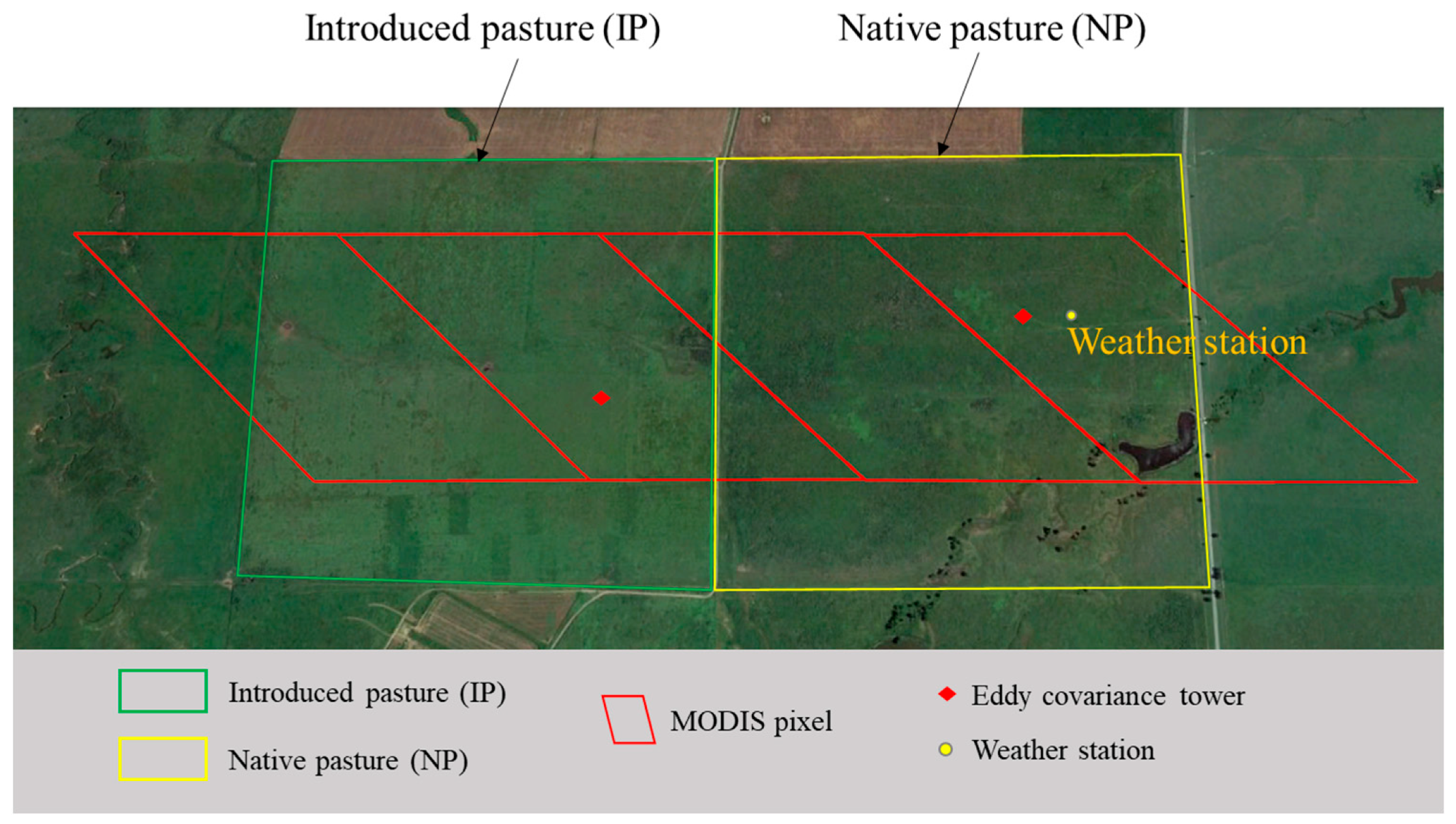
2.1. Study Area
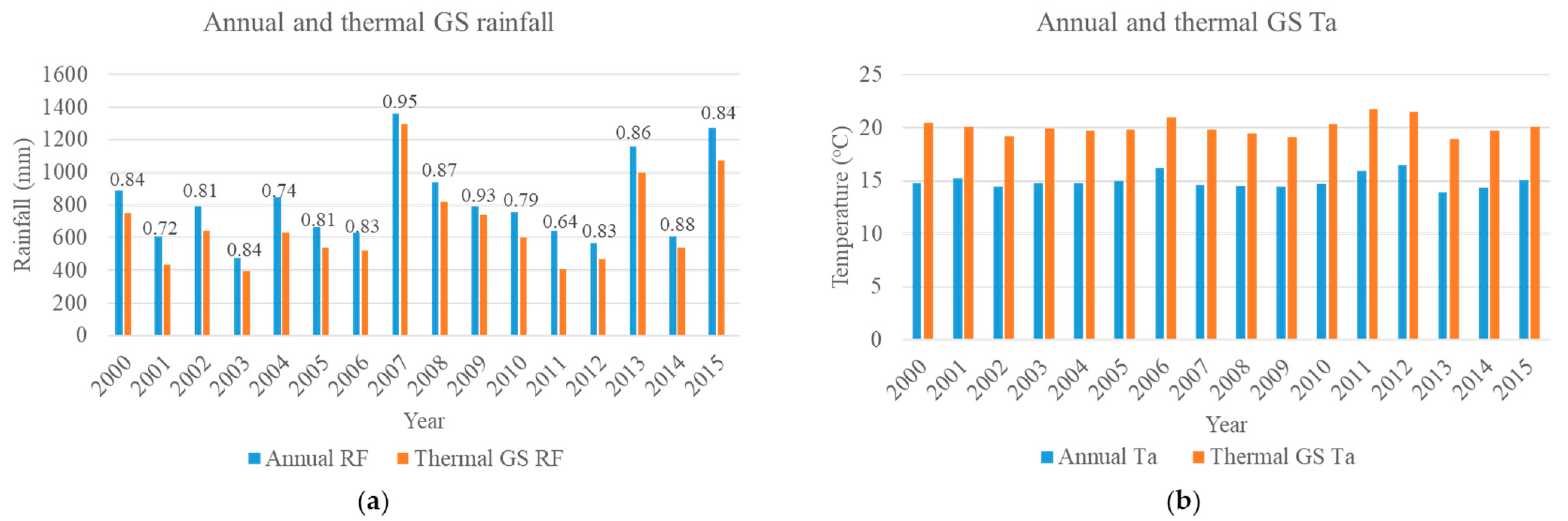
2.2. Climate Data
2.3. Management Records for the Native and Introduced Pastures
2.4. MODIS and Landsat Images and Vegetation Indices
2.5. Vegetation Phenology Metrics and Greenness Derived from MODIS Vegetation Indices
2.6. Gross Primary Production (GPP) Estimates from the Vegetation Photosynthesis Model
2.7. Statistical Analysis
3. Results
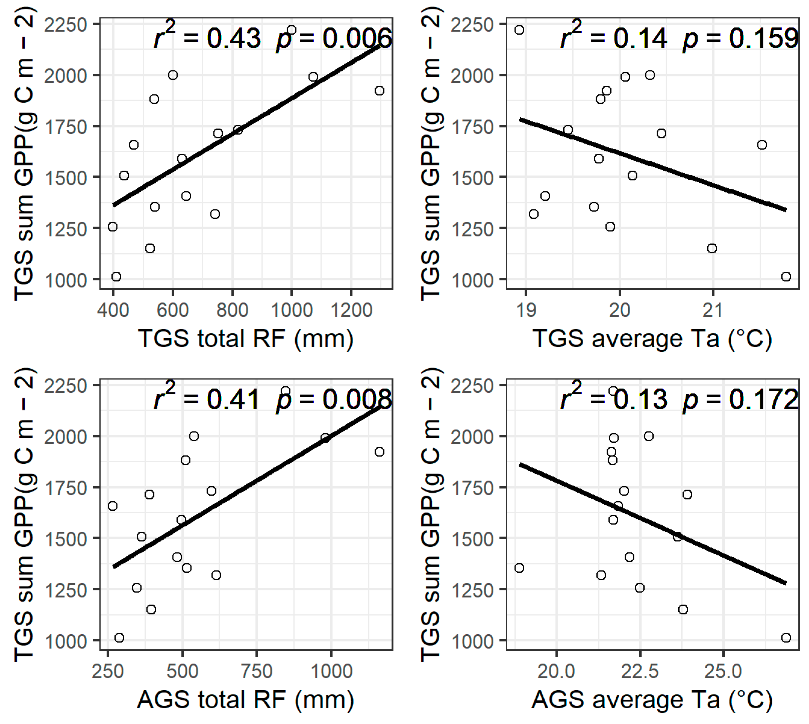
3.1. Relationships of Vegetation Phenology, Greenness, and GPP with Climate Factors
3.2. Intra-Annual Dynamics of Vegetation Phenology Affected by a Single Factor
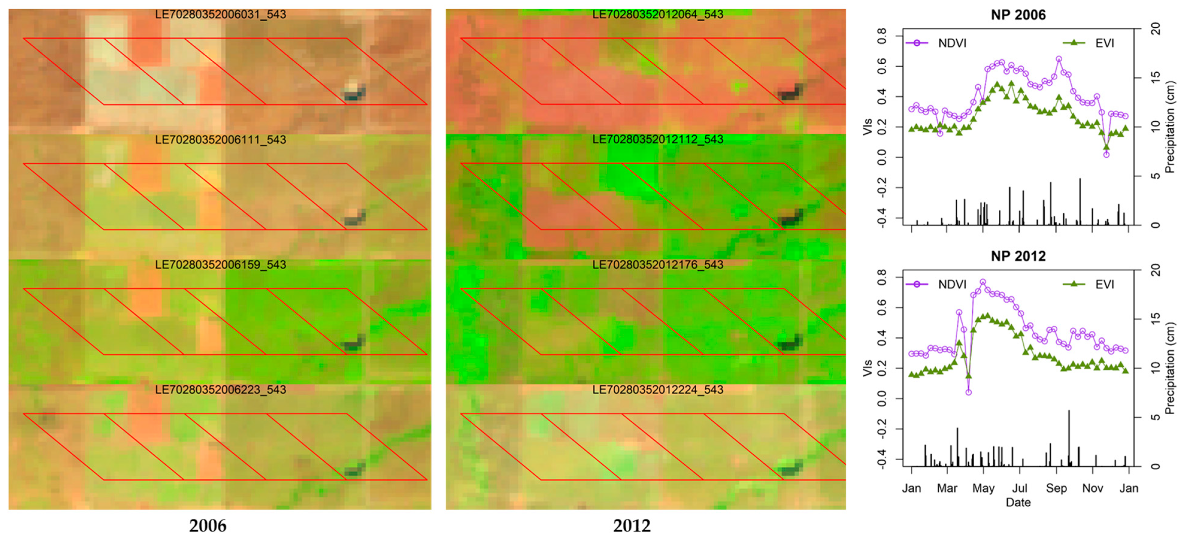
3.2.1. Impacts of Drought in the NP
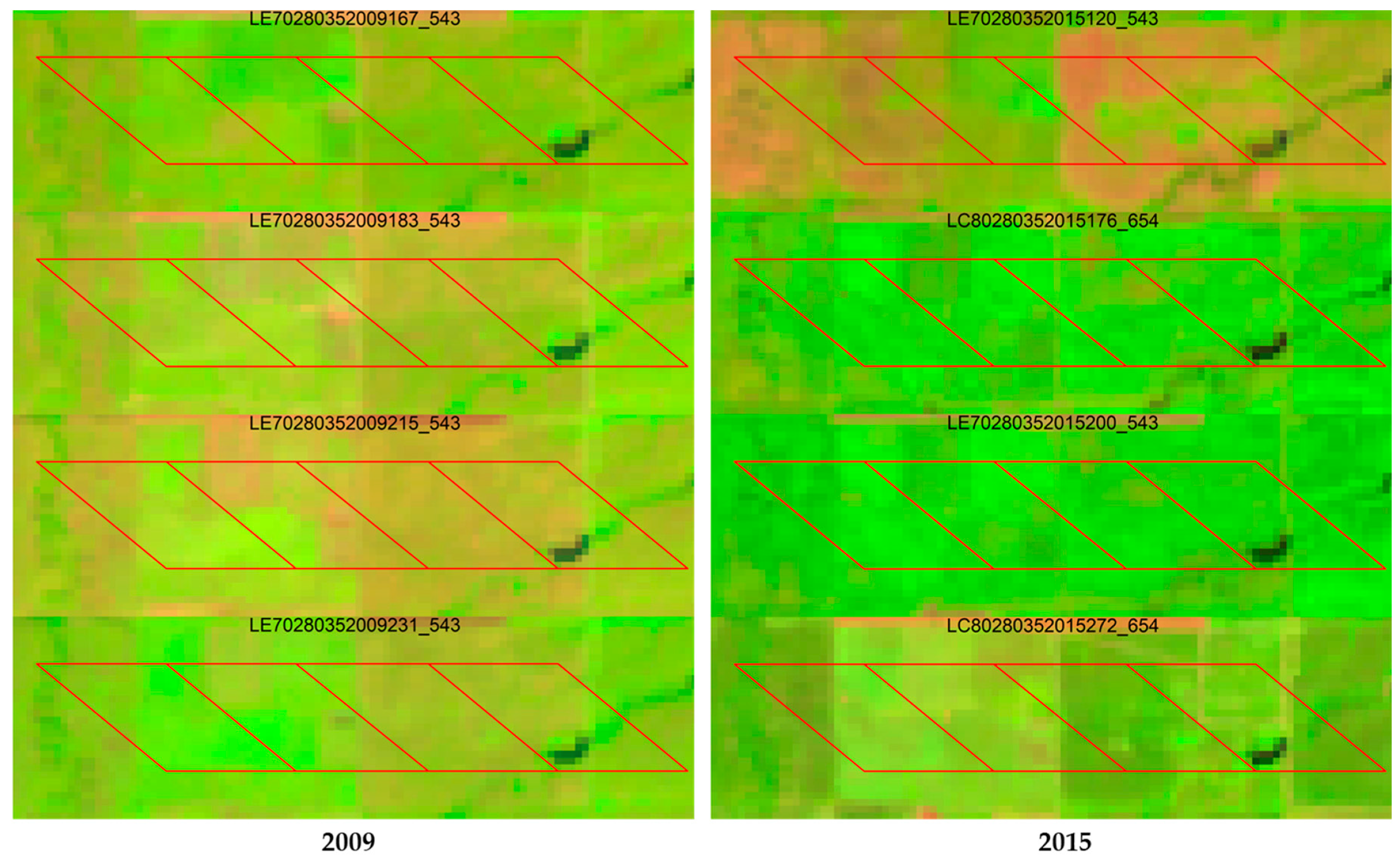
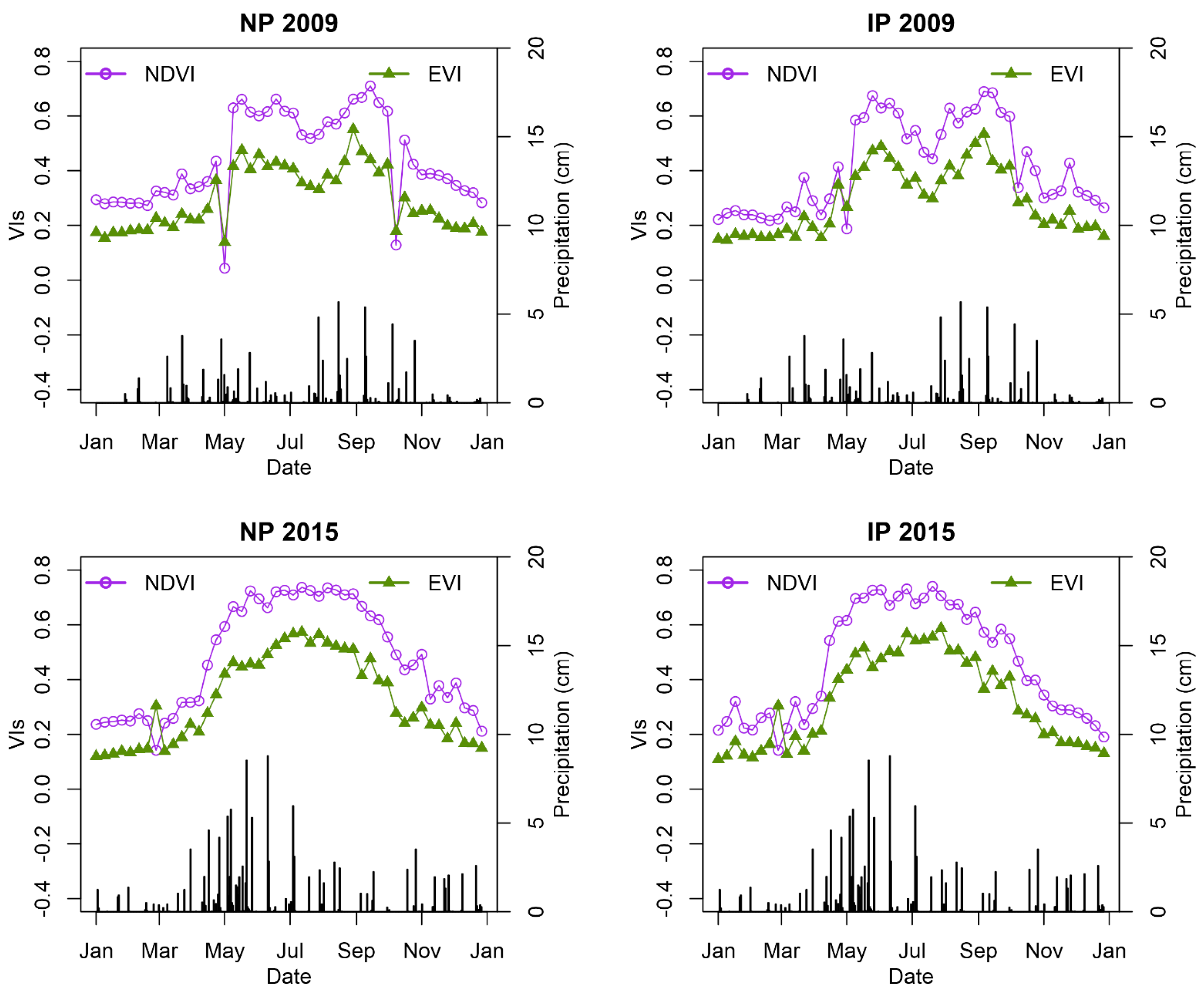
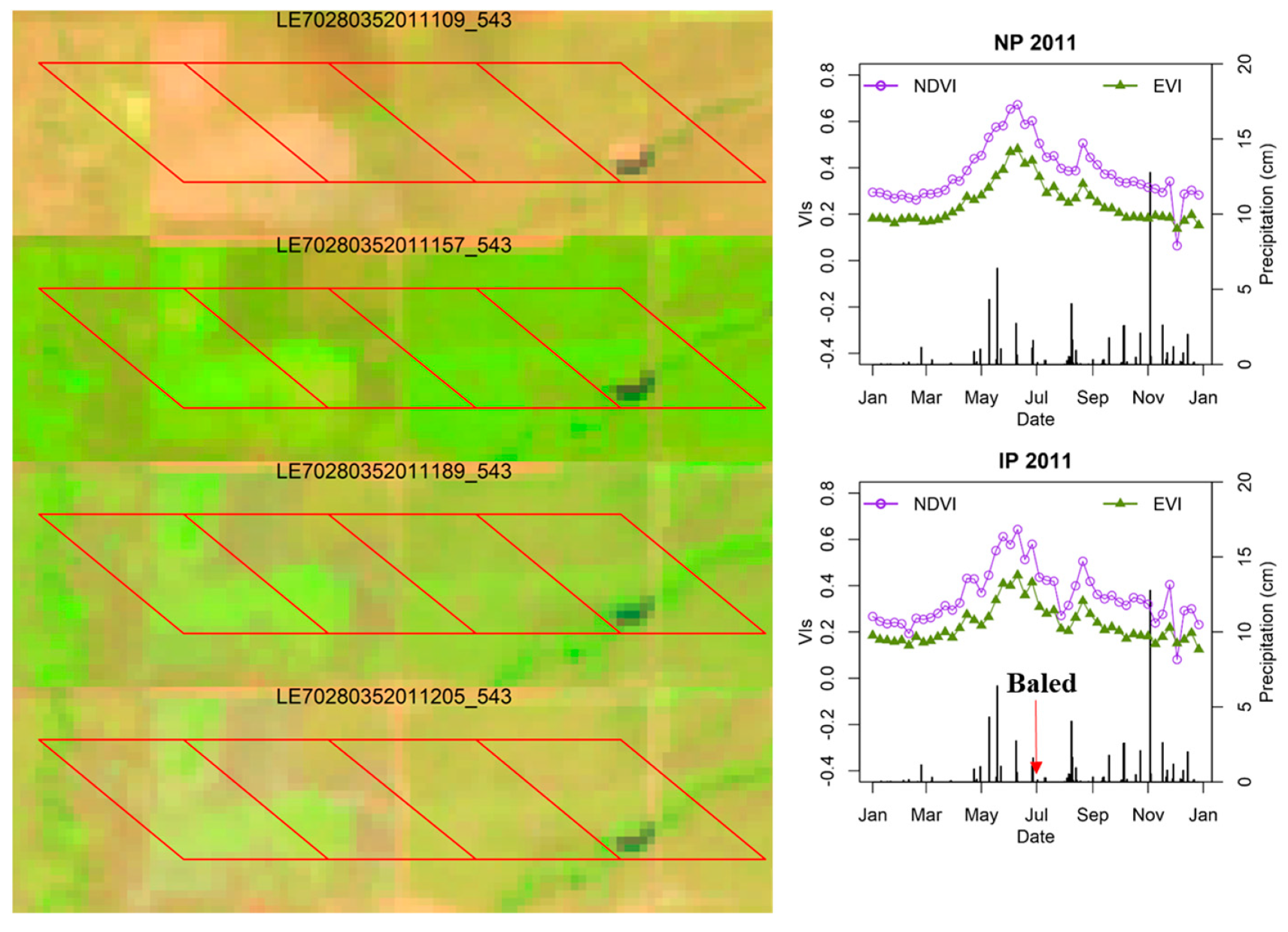
3.2.2. Impacts of Grazing in the NP and IP
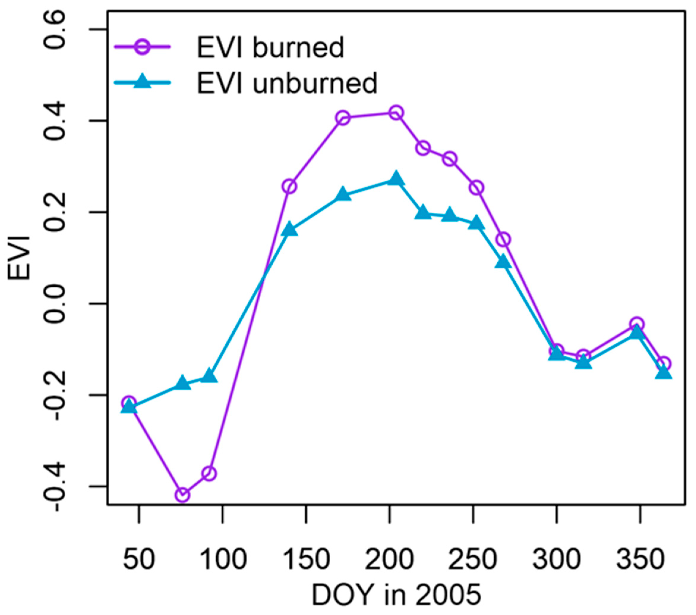
3.2.3. Impacts of Burning in the NP and IP
3.3. Impacts of Climate and Management Interactions on Vegetation Phenology and GPP
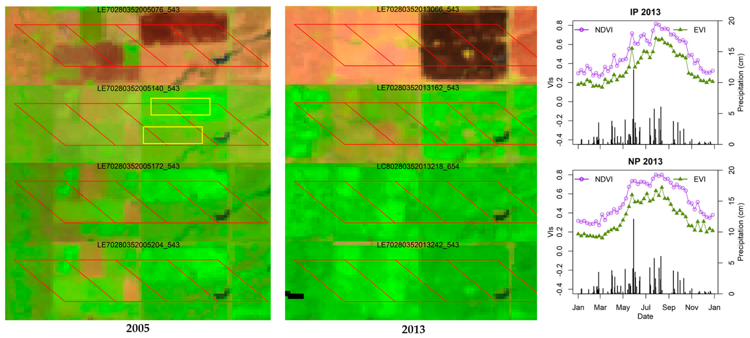
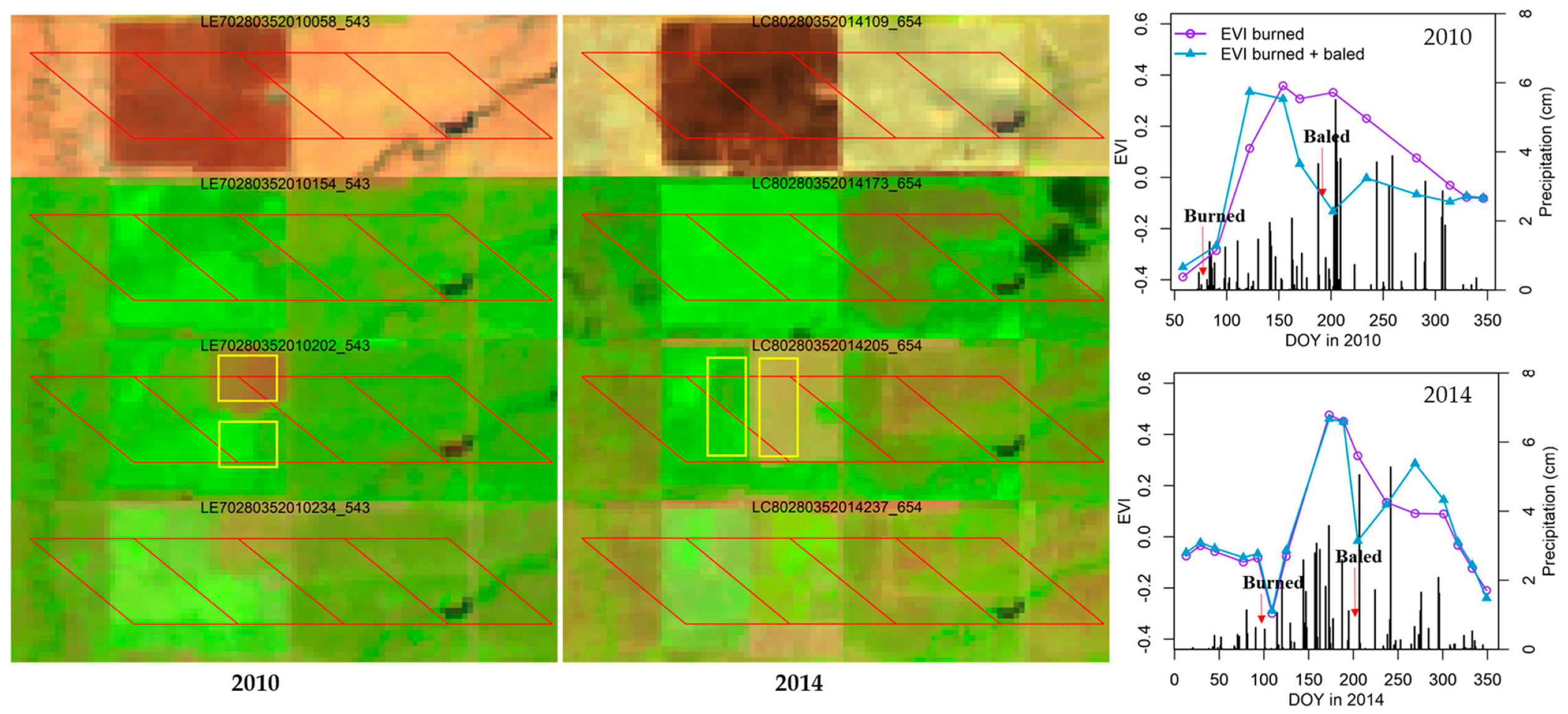
3.3.1. Interactions of Burning plus Baling with RF in the IP
3.3.2. Drought plus Grazing in the NP and Drought plus Baling in the IP
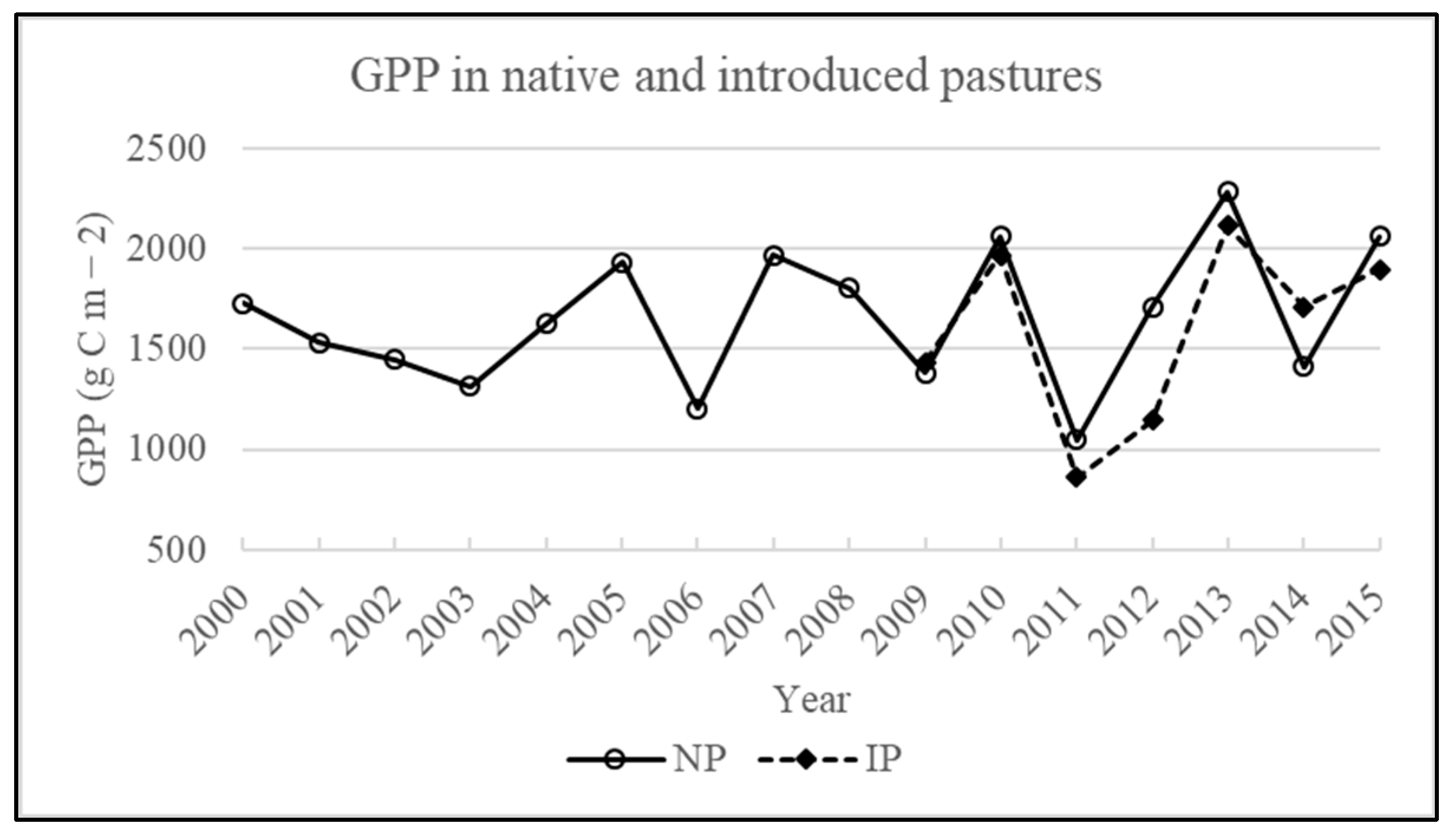
3.3.3. Summary of Vegetation Phenology and GPP under Different Climate and Management
4. Discussion
4.1. Combination of MODIS and Landsat to Study Vegetation Phenology and Production
4.2. The Impacts of Climate and Management Interactions on Vegetation Phenology and GPP
4.3. Implications and Future Steps
5. Conclusions
Author Contributions
Funding
Data Availability Statement
Conflicts of Interest
References
- Menzel, A. Phenology: Its importance to the global change community. Clim. Chang. 2002, 54, 379–385. [Google Scholar] [CrossRef]
- White, M.A.; Thornton, P.E.; Running, S.W. A continental phenology model for monitoring vegetation responses to interannual climatic variability. Glob. Biogeochem. Cycles 1997, 11, 217–234. [Google Scholar] [CrossRef]
- Cao, M.; Woodward, F.I. Dynamic responses of terrestrial ecosystem carbon cycling to global climate change. Nature 1998, 393, 249–252. [Google Scholar] [CrossRef]
- Peñuelas, J.; Filella, I. Responses to a warming world. Science 2001, 294, 793–795. [Google Scholar] [CrossRef]
- Zhang, X.; Friedl, M.A.; Schaaf, C.B. Global vegetation phenology from Moderate Resolution Imaging Spectroradiometer (MODIS): Evaluation of global patterns and comparison with in situ measurements. J. Geophys. Res. Biogeosci. 2006, 111, G04017. [Google Scholar] [CrossRef]
- Fisher, J.I.; Mustard, J.F. Cross-scalar satellite phenology from ground, Landsat, and MODIS data. Remote Sens. Environ. 2007, 109, 261–273. [Google Scholar] [CrossRef]
- Ganguly, S.; Friedl, M.A.; Tan, B.; Zhang, X.; Verma, M. Land surface phenology from MODIS: Characterization of the Collection 5 global land cover dynamics product. Remote Sens. Environ. 2010, 114, 1805–1816. [Google Scholar] [CrossRef]
- Walker, J.J.; de Beurs, K.M.; Wynne, R.H.; Gao, F. Evaluation of Landsat and MODIS data fusion products for analysis of dryland forest phenology. Remote Sens. Environ. 2012, 117, 381–393. [Google Scholar] [CrossRef]
- Forkel, M.; Migliavacca, M.; Thonicke, K.; Reichstein, M.; Schaphoff, S.; Weber, U.; Carvalhais, N. Codominant water control on global interannual variability and trends in land surface phenology and greenness. Glob. Chang. Biol. 2015, 21, 3414–3435. [Google Scholar] [CrossRef]
- Zeng, L.; Wardlow, B.D.; Wang, R.; Shan, J.; Tadesse, T.; Hayes, M.J.; Li, D. A hybrid approach for detecting corn and soybean phenology with time-series MODIS data. Remote Sens. Environ. 2016, 181, 237–250. [Google Scholar] [CrossRef]
- Moulin, S.; Kergoat, L.; Viovy, N.; Dedieu, G. Global-scale assessment of vegetation phenology using NOAA/AVHRR satellite measurements. J. Clim. 1997, 10, 1154–1170. [Google Scholar] [CrossRef]
- Delbart, N.; Kergoat, L.; Le Toan, T.; Lhermitte, J.; Picard, G. Determination of phenological dates in boreal regions using normalized difference water index. Remote Sens. Environ. 2005, 97, 26–38. [Google Scholar] [CrossRef]
- Fisher, J.I.; Mustard, J.F.; Vadeboncoeur, M.A. Green leaf phenology at Landsat resolution: Scaling from the field to the satellite. Remote Sens. Environ. 2006, 100, 265–279. [Google Scholar] [CrossRef]
- Sakamoto, T.; Yokozawa, M.; Toritani, H.; Shibayama, M.; Ishitsuka, N.; Ohno, H. A crop phenology detection method using time-series MODIS data. Remote Sens. Environ. 2005, 96, 366–374. [Google Scholar] [CrossRef]
- Atzberger, C.; Klisch, A.; Mattiuzzi, M.; Vuolo, F. Phenological metrics derived over the European continent from NDVI3g data and MODIS time series. Remote Sens. 2014, 6, 257–284. [Google Scholar] [CrossRef]
- Zhang, G.; Zhang, Y.; Dong, J.; Xiao, X. Green-up dates in the Tibetan Plateau have continuously advanced from 1982 to 2011. Proc. Natl. Acad. Sci. USA 2013, 110, 4309–4314. [Google Scholar] [CrossRef]
- Rouse, J.W., Jr.; Haas, R.; Schell, J.; Deering, D. Monitoring vegetation systems in the great plains with erts. NASA Spec. Publ. 1974, 351, 309. [Google Scholar]
- Tucker, C.J. Red and photographic infrared linear combinations for monitoring vegetation. Remote Sens. Environ. 1979, 8, 127–150. [Google Scholar] [CrossRef]
- Wang, J.; Price, K.P.; Rich, P.M. Spatial patterns of NDVI in response to precipitation and temperature in the central Great Plains. Int. J. Remote Sens. 2001, 22, 3827–3844. [Google Scholar] [CrossRef]
- Pettorelli, N.; Vik, J.O.; Mysterud, A.; Gaillard, J.-M.; Tucker, C.J.; Stenseth, N.C. Using the satellite-derived NDVI to assess ecological responses to environmental change. Trends Ecol. Evol. 2005, 20, 503–510. [Google Scholar] [CrossRef]
- Massey, R.; Sankey, T.T.; Congalton, R.G.; Yadav, K.; Thenkabail, P.S.; Ozdogan, M.; Sánchez Meador, A.J. MODIS phenology-derived, multi-year distribution of conterminous U.S. crop types. Remote Sens. Environ. 2017, 198, 490–503. [Google Scholar] [CrossRef]
- Huete, A.; Didan, K.; Miura, T.; Rodriguez, E.P.; Gao, X.; Ferreira, L.G. Overview of the radiometric and biophysical performance of the MODIS vegetation indices. Remote Sens. Environ. 2002, 83, 195–213. [Google Scholar] [CrossRef]
- Zhang, X.; Friedl, M.A.; Schaaf, C.B.; Strahler, A.H.; Liu, Z. Monitoring the response of vegetation phenology to precipitation in Africa by coupling MODIS and TRMM instruments. J. Geophys. Res. Atmos. 2005, 110, D12103. [Google Scholar] [CrossRef]
- Liu, Y.; Wu, C.; Peng, D.; Xu, S.; Gonsamo, A.; Jassal, R.S.; Altaf Arain, M.; Lu, L.; Fang, B.; Chen, J.M. Improved modeling of land surface phenology using MODIS land surface reflectance and temperature at evergreen needleleaf forests of central North America. Remote Sens. Environ. 2016, 176, 152–162. [Google Scholar] [CrossRef]
- Hird, J.N.; McDermid, G.J. Noise reduction of NDVI time series: An empirical comparison of selected techniques. Remote Sens. Environ. 2009, 113, 248–258. [Google Scholar] [CrossRef]
- Verbesselt, J.; Hyndman, R.; Zeileis, A.; Culvenor, D. Phenological change detection while accounting for abrupt and gradual trends in satellite image time series. Remote Sens. Environ. 2010, 114, 2970–2980. [Google Scholar] [CrossRef]
- Tan, B.; Morisette, J.T.; Wolfe, R.E.; Gao, F.; Ederer, G.A.; Nightingale, J.; Pedelty, J.A. An Enhanced TIMESAT Algorithm for Estimating Vegetation Phenology Metrics From MODIS Data. IEEE J. Sel. Top. Appl. Earth Obs. Remote Sens. 2011, 4, 361–371. [Google Scholar] [CrossRef]
- Jönsson, P.; Eklundh, L. TIMESAT—A program for analyzing time-series of satellite sensor data. Comput. Geosci. 2004, 30, 833–845. [Google Scholar] [CrossRef]
- Julien, Y.; Sobrino, J. Global land surface phenology trends from GIMMS database. Int. J. Remote Sens. 2009, 30, 3495–3513. [Google Scholar] [CrossRef]
- Keenan, T.F.; Gray, J.; Friedl, M.A.; Toomey, M.; Bohrer, G.; Hollinger, D.Y.; Munger, J.W.; O’Keefe, J.; Schmid, H.P.; Wing, I.S. Net carbon uptake has increased through warming-induced changes in temperate forest phenology. Nat. Clim. Chang. 2014, 4, 598–604. [Google Scholar] [CrossRef]
- Goetz, S.J.; Bunn, A.G.; Fiske, G.J.; Houghton, R. Satellite-observed photosynthetic trends across boreal North America associated with climate and fire disturbance. Proc. Natl. Acad. Sci. USA 2005, 102, 13521–13525. [Google Scholar] [CrossRef]
- Verbesselt, J.; Hyndman, R.; Newnham, G.; Culvenor, D. Detecting trend and seasonal changes in satellite image time series. Remote Sens. Environ. 2010, 114, 106–115. [Google Scholar] [CrossRef]
- Mildrexler, D.J.; Zhao, M.; Heinsch, F.A.; Running, S.W. A new satellite-based methodology for continental-scale disturbance detection. Ecol. Appl. 2007, 17, 235–250. [Google Scholar] [CrossRef]
- Mildrexler, D.J.; Zhao, M.; Running, S.W. Testing a MODIS Global Disturbance Index across North America. Remote Sens. Environ. 2009, 113, 2103–2117. [Google Scholar] [CrossRef]
- Vermote, E.; Vermeulen, A. Atmospheric Correction Algorithm: Spectral Reflectances (MOD09); Version 4; Department of Geography, University of Maryland: College Park, MD, USA, 1999. [Google Scholar]
- Cohen, W.B.; Spies, T.A.; Alig, R.J.; Oetter, D.R.; Maiersperger, T.K.; Fiorella, M. Characterizing 23 Years (1972–1995) of Stand Replacement Disturbance in Western Oregon Forests with Landsat Imagery. Ecosystems 2002, 5, 122–137. [Google Scholar] [CrossRef]
- Zhou, Y.; Xiao, X.; Wagle, P.; Bajgain, R.; Mahan, H.; Basara, J.B.; Dong, J.; Qin, Y.; Zhang, G.; Luo, Y.; et al. Examining the short-term impacts of diverse management practices on plant phenology and carbon fluxes of Old World bluestems pasture. Agric. For. Meteorol. 2017, 237–238, 60–70. [Google Scholar] [CrossRef]
- Schubert, S.D.; Suarez, M.J.; Pegion, P.J.; Koster, R.D.; Bacmeister, J.T. On the cause of the 1930s Dust Bowl. Science 2004, 303, 1855–1859. [Google Scholar] [CrossRef]
- Hoerling, M.; Eischeid, J.; Kumar, A.; Leung, R.; Mariotti, A.; Mo, K.; Schubert, S.; Seager, R. Causes and predictability of the 2012 Great Plains drought. Bull. Am. Meteorol. Soc. 2014, 95, 269–282. [Google Scholar] [CrossRef]
- Gu, Y.; Hunt, E.; Wardlow, B.; Basara, J.B.; Brown, J.F.; Verdin, J.P. Evaluation of MODIS NDVI and NDWI for vegetation drought monitoring using Oklahoma Mesonet soil moisture data. Geophys. Res. Lett. 2008, 35, L22401. [Google Scholar] [CrossRef]
- Gu, Y.; Brown, J.F.; Verdin, J.P.; Wardlow, B. A five-year analysis of MODIS NDVI and NDWI for grassland drought assessment over the central Great Plains of the United States. Geophys. Res. Lett. 2007, 34, L06407. [Google Scholar] [CrossRef]
- Christian, J.; Christian, K.; Basara, J.B. Drought and pluvial dipole events within the great plains of the United States. J. Appl. Meteorol. Climatol. 2015, 54, 1886–1898. [Google Scholar] [CrossRef]
- Basara, J.B.; Maybourn, J.N.; Peirano, C.M.; Tate, J.E.; Brown, P.J.; Hoey, J.D.; Smith, B.R. Drought and associated impacts in the Great Plains of the United States—A review. Int. J. Geosci. 2013, 4, 72. [Google Scholar] [CrossRef]
- Zhou, Y.; Xiao, X.; Zhang, G.; Wagle, P.; Bajgain, R.; Dong, J.; Jin, C.; Basara, J.B.; Anderson, M.C.; Hain, C.; et al. Quantifying agricultural drought in tallgrass prairie region in the U.S. Southern Great Plains through analysis of a water-related vegetation index from MODIS images. Agric. For. Meteorol. 2017, 246, 111–122. [Google Scholar] [CrossRef]
- Brockway, D.G.; Gatewood, R.G.; Paris, R.B. Restoring fire as an ecological process in shortgrass prairie ecosystems: Initial effects of prescribed burning during the dormant and growing seasons. J. Environ. Manag. 2002, 65, 135–152. [Google Scholar] [CrossRef] [PubMed]
- Twidwell, D.; Rogers, W.E.; Fuhlendorf, S.D.; Wonkka, C.L.; Engle, D.M.; Weir, J.R.; Kreuter, U.P.; Taylor, C.A. The rising Great Plains fire campaign: Citizens’ response to woody plant encroachment. Front. Ecol. Environ. 2013, 11, e64–e71. [Google Scholar] [CrossRef]
- Reinhart, K.O.; Dangi, S.R.; Vermeire, L.T. The effect of fire intensity, nutrients, soil microbes, and spatial distance on grassland productivity. Plant Soil 2016, 409, 203–216. [Google Scholar] [CrossRef]
- Wagle, P.; Gowda, P.H.; Northup, B.K.; Starks, P.J.; Neel, J.P. Response of tallgrass prairie to management in the US Southern Great Plains: Site descriptions, management practices, and eddy covariance instrumentation for a long-term experiment. Remote Sens. 2019, 11, 1988. [Google Scholar] [CrossRef]
- Campioli, M.; Vicca, S.; Luyssaert, S.; Bilcke, J.; Ceschia, E.; Chapin, F., III; Ciais, P.; Fernández-Martínez, M.; Malhi, Y.; Obersteiner, M. Biomass production efficiency controlled by management in temperate and boreal ecosystems. Nat. Geosci. 2015, 8, 843–846. [Google Scholar] [CrossRef]
- Wagle, P.; Xiao, X.; Torn, M.S.; Cook, D.R.; Matamala, R.; Fischer, M.L.; Jin, C.; Dong, J.; Biradar, C. Sensitivity of vegetation indices and gross primary production of tallgrass prairie to severe drought. Remote Sens. Environ. 2014, 152, 1–14. [Google Scholar] [CrossRef]
- McPherson, R.A.; Fiebrich, C.A.; Crawford, K.C.; Kilby, J.R.; Grimsley, D.L.; Martinez, J.E.; Basara, J.B.; Illston, B.G.; Morris, D.A.; Kloesel, K.A. Statewide monitoring of the mesoscale environment: A technical update on the Oklahoma Mesonet. J. Atmos. Ocean. Technol. 2007, 24, 301–321. [Google Scholar] [CrossRef]
- Bajgain, R.; Xiao, X.; Basara, J.B.; Wagle, P.; Zhou, Y.; Mahan, H.; Gowda, P.H.; McCarthy, H.R.; Northup, B.; Neel, J.P.S.; et al. Carbon dioxide and water vapor fluxes in winter wheat and tallgrass prairie in central Oklahoma. Sci. Total Environ. 2018, 644, 1511–1524. [Google Scholar] [CrossRef]
- Zhou, Y.; Xiao, X.; Qin, Y.; Dong, J.; Zhang, G.; Kou, W.; Jin, C.; Wang, J.; Li, X. Mapping paddy rice planting area in rice-wetland coexistent areas through analysis of Landsat 8 OLI and MODIS images. Int. J. Appl. Earth Obs. Geoinf. 2016, 46, 1–12. [Google Scholar] [CrossRef]
- Xiao, X.; Hollinger, D.; Aber, J.; Goltz, M.; Davidson, E.A.; Zhang, Q.; Moore, B. Satellite-based modeling of gross primary production in an evergreen needleleaf forest. Remote Sens. Environ. 2004, 89, 519–534. [Google Scholar] [CrossRef]
- Bajgain, R.; Xiao, X.; Basara, J.; Doughty, R.; Wu, X.; Wagle, P.; Zhou, Y.; Gowda, P.; Steiner, J. Differential responses of native and managed prairie pastures to environmental variability and management practices. Agric. For. Meteorol. 2020, 294, 108137. [Google Scholar] [CrossRef]
- Otkin, J.A.; Anderson, M.C.; Hain, C.; Svoboda, M.; Johnson, D.; Mueller, R.; Tadesse, T.; Wardlow, B.; Brown, J. Assessing the evolution of soil moisture and vegetation conditions during the 2012 United States flash drought. Agric. For. Meteorol. 2016, 218, 230–242. [Google Scholar] [CrossRef]
- Rogiers, N.; Eugster, W.; Furger, M.; Siegwolf, R. Effect of land management on ecosystem carbon fluxes at a subalpine grassland site in the Swiss Alps. Theor. Appl. Climatol. 2005, 80, 187–203. [Google Scholar] [CrossRef]
- Zeeman, M.J.; Hiller, R.; Gilgen, A.K.; Michna, P.; Plüss, P.; Buchmann, N.; Eugster, W. Management and climate impacts on net CO2 fluxes and carbon budgets of three grasslands along an elevational gradient in Switzerland. Agric. For. Meteorol. 2010, 150, 519–530. [Google Scholar] [CrossRef]
- Kennedy, R.E.; Andréfouët, S.; Cohen, W.B.; Gómez, C.; Griffiths, P.; Hais, M.; Healey, S.P.; Helmer, E.H.; Hostert, P.; Lyons, M.B.; et al. Bringing an ecological view of change to Landsat-based remote sensing. Front. Ecol. Environ. 2014, 12, 339–346. [Google Scholar] [CrossRef]
- McDowell, N.G.; Coops, N.C.; Beck, P.S.A.; Chambers, J.Q.; Gangodagamage, C.; Hicke, J.A.; Huang, C.-Y.; Kennedy, R.; Krofcheck, D.J.; Litvak, M.; et al. Global satellite monitoring of climate-induced vegetation disturbances. Trends Plant Sci. 2015, 20, 114–123. [Google Scholar] [CrossRef]
- Hansen, M.C.; Potapov, P.V.; Moore, R.; Hancher, M.; Turubanova, S.; Tyukavina, A.; Thau, D.; Stehman, S.; Goetz, S.; Loveland, T. High-resolution global maps of 21st-century forest cover change. Science 2013, 342, 850–853. [Google Scholar] [CrossRef]
- Gorelick, N.; Hancher, M.; Dixon, M.; Ilyushchenko, S.; Thau, D.; Moore, R. Google Earth Engine: Planetary-scale geospatial analysis for everyone. Remote Sens. Environ. 2017, 202, 18–27. [Google Scholar] [CrossRef]
- Robinson, N.P.; Allred, B.W.; Jones, M.O.; Moreno, A.; Kimball, J.S.; Naugle, D.E.; Erickson, T.A.; Richardson, A.D. A Dynamic Landsat Derived Normalized Difference Vegetation Index (NDVI) Product for the Conterminous United States. Remote Sens. 2017, 9, 863. [Google Scholar] [CrossRef]
- Suyker, A.E.; Verma, S.B.; Burba, G.G. Interannual variability in net CO2 exchange of a native tallgrass prairie. Glob. Chang. Biol. 2003, 9, 255–265. [Google Scholar] [CrossRef]
- Fischer, M.L.; Torn, M.S.; Billesbach, D.P.; Doyle, G.; Northup, B.; Biraud, S.C. Carbon, water, and heat flux responses to experimental burning and drought in a tallgrass prairie. Agric. For. Meteorol. 2012, 166–167, 169–174. [Google Scholar] [CrossRef]
- Wagle, P.; Kakani, V.G.; Gowda, P.H.; Xiao, X.; Northup, B.K.; Neel, J.P.; Starks, P.J.; Steiner, J.L.; Gunter, S.A. Dormant Season Vegetation Phenology and Eddy Fluxes in Native Tallgrass Prairies of the US Southern Plains. Remote Sens. 2022, 14, 2620. [Google Scholar] [CrossRef]
- Flynn, K.C.; Zhou, Y.; Gowda, P.H.; Moffet, C.A.; Wagle, P.; Kakani, V.G. Burning and Climate Interactions Determine Impacts of Grazing on Tallgrass Prairie Systems. Rangel. Ecol. Manag. 2020, 73, 104–118. [Google Scholar] [CrossRef]
- Running, S.W.; Baldocchi, D.D.; Turner, D.P.; Gower, S.T.; Bakwin, P.S.; Hibbard, K.A. A Global Terrestrial Monitoring Network Integrating Tower Fluxes, Flask Sampling, Ecosystem Modeling and EOS Satellite Data. Remote Sens. Environ. 1999, 70, 108–127. [Google Scholar] [CrossRef]
- Zhou, Y.; Flynn, K.C.; Gowda, P.H.; Wagle, P.; Ma, S.; Kakani, V.G.; Steiner, J.L. The potential of active and passive remote sensing to detect frequent harvesting of alfalfa. Int. J. Appl. Earth Obs. Geoinf. 2021, 104, 102539. [Google Scholar] [CrossRef]


| Year | Native Pasture | Introduced Pasture |
|---|---|---|
| 2009 | (1). Stocking rate 0.39 head/ha for May–October | (1). Burned on 15 April 2009; (2). May~1st, Weed control and fertiliza-tion (3). July~1st, Hayed |
| 2010 | (1). Stocking rate 0.37 head/ha for May–October | (1). Burned on 18 March 2010; (2). July~1st, Hayed |
| 2011 | (1). Stocking rate 0.45 head/ha for May–October | (1). July~1st, Hayed |
| 2012 | Rested all year | (1). Stock rate 0.83 hd/ha for January–May and 0.32 hd/ha for June–July |
| 2013 | (1). Burned on 3/6/2013; (2). Stocking rate 0.78 head/ha for December | (1). Stock rate of 0.64 hd/ha for January–March |
| 2014 | (1). Stocking rate 0.78 head/ha for April, May, July and November | (1). 9 April 2014 Burned; (2). 7/23 60% of East half of pasture cut for hay, 8/15 40% of East half of pasture cut for hay; (3). Stock rate of 0.40 hd/ha for September–December |
| 2015 | (1). Stocking rate 0.78 head/ha for February and 0.39 head/ha for June–July | (1). Stock rate of 0.40 hd/ha for January–February and June–July; (2). Stock rate of 0.96 hd/ha for August–December |
| SOS (NDVI/EVI-based) | Early season total RF |
| Early season average Ta | |
| Early season maximum Ta | |
| EOS (NDVI/EVI-based) | Late season total RF |
| Late season average Ta | |
| LOS (NDVI/EVI-based) | Thermal GS total RF |
| Thermal GS average Ta | |
| Annual GS total RF | |
| Annual GS average Ta | |
| Peak NDVI/EVI | Early season total RF |
| Early season average Ta | |
| NDVI/EVI sum | Thermal GS total RF |
| Thermal GS average Ta | |
| Annual GS total RF | |
| Annual GS average Ta | |
| NDVI/EVI average | Thermal GS total RF |
| Thermal GS average Ta | |
| Annual GS total RF | |
| Annual GS average Ta |
| Year | Disturbance Type | Pastures | SOS (DOY) | EOS (DOY) | LOS (Days) | GS EVI Average | GS EVI Sum | GPP (g C m−2) | AGS Rainfall (cm) |
|---|---|---|---|---|---|---|---|---|---|
| 2015 | Three month grazing | NP | 113 | 290 | 178 | 0.48 | 10.92 | 2062.18 | 86.56 |
| Whole year grazing | IP | 110 | 293 | 182 | 0.47 | 11.36 | 1895.86 | ||
| 2014 | Four month grazing | NP | 141 | 310 | 169 | 0.38 | 8.35 | 1411.02 | 45.80 |
| Burning + baling | IP | 133 | 282 | 149 | 0.48 | 9.16 | 1711.64 | ||
| 2013 | Burning | NP | 131 | 294 | 162 | 0.52 | 11.35 | 2281.61 | 82.55 |
| None | IP | 137 | 304 | 167 | 0.52 | 11.49 | 2111.77 | ||
| 2012 | Drought | NP | 85 | 212 | 128 | 0.45 | 7.24 | 1709.79 | 20.80 |
| Drought + grazing | IP | 93 | 209 | 116 | 0.41 | 6.10 | 1143.39 | ||
| 2011 | Drought + grazing | NP | 128 | 253 | 125 | 0.35 | 5.95 | 1049.30 | 27.71 |
| Drought + baling | IP | 131 | 257 | 126 | 0.33 | 5.59 | 863.00 | ||
| 2010 | Six month grazing | NP | 114 | 293 | 180 | 0.46 | 11.09 | 2059.05 | 47.00 |
| Burning + baling | IP | 110 | 291 | 181 | 0.51 | 11.66 | 1965.43 | ||
| 2009 | Six month grazing | NP | 116 | 297 | 181 | 0.40 | 9.66 | 1382.18 | 57.91 |
| Burning + baling | IP | 128 | 296 | 168 | 0.41 | 9.09 | 1435.70 | ||
| 2006 | Drought | NP | 119 | 282 | 163 | 0.38 | 7.98 | 1204.27 | 37.11 |
Disclaimer/Publisher’s Note: The statements, opinions and data contained in all publications are solely those of the individual author(s) and contributor(s) and not of MDPI and/or the editor(s). MDPI and/or the editor(s) disclaim responsibility for any injury to people or property resulting from any ideas, methods, instructions or products referred to in the content. |
© 2023 by the authors. Licensee MDPI, Basel, Switzerland. This article is an open access article distributed under the terms and conditions of the Creative Commons Attribution (CC BY) license (https://creativecommons.org/licenses/by/4.0/).
Share and Cite
Zhou, Y.; Ma, S.; Wagle, P.; Gowda, P.H. Climate and Management Practices Jointly Control Vegetation Phenology in Native and Introduced Prairie Pastures. Remote Sens. 2023, 15, 2529. https://doi.org/10.3390/rs15102529
Zhou Y, Ma S, Wagle P, Gowda PH. Climate and Management Practices Jointly Control Vegetation Phenology in Native and Introduced Prairie Pastures. Remote Sensing. 2023; 15(10):2529. https://doi.org/10.3390/rs15102529
Chicago/Turabian StyleZhou, Yuting, Shengfang Ma, Pradeep Wagle, and Prasanna H. Gowda. 2023. "Climate and Management Practices Jointly Control Vegetation Phenology in Native and Introduced Prairie Pastures" Remote Sensing 15, no. 10: 2529. https://doi.org/10.3390/rs15102529