Article

Estimates of Hyperspectral Surface and Underwater UV Planar and Scalar Irradiances from OMI Measurements and Radiative Transfer Computations

1
Science Systems and Applications, Inc., 10210 Greenbelt Road, Lanham, MD 20706, USA
2
NASA Goddard Space Flight Center, Greenbelt, MD 20771, USA
*
Author to whom correspondence should be addressed.
Remote Sens. 2022, 14(9), 2278; https://doi.org/10.3390/rs14092278
Submission received: 1 April 2022 / Revised: 1 May 2022 / Accepted: 3 May 2022 / Published: 9 May 2022
(This article belongs to the Topic Advances in Environmental Remote Sensing)

Abstract

:
Quantitative assessment of the UV effects on aquatic ecosystems requires an estimate of the in-water hyperspectral radiation field. Solar UV radiation in ocean waters is estimated on a global scale by combining extraterrestrial solar irradiance from the Total and Spectral Solar Irradiance Sensor (TSIS-1), satellite estimates of cloud/surface reflectivity, ozone from the Ozone Monitoring Instrument (OMI) and in-water chlorophyll concentration from the Moderate Resolution Imaging Spectroradiometer (MODIS) with radiative transfer computations in the ocean-atmosphere system. A comparison of the estimates of collocated OMI-derived surface irradiance with Marine Optical Buoy (MOBY) measurements shows a good agreement within 5% for different seasons. To estimate scalar irradiance at the ocean surface and in water, we propose scaling the planar irradiance, calculated from satellite observation, on the basis of Hydrolight computations. Hydrolight calculations show that the diffuse attenuation coefficients of scalar and planar irradiance with depth are quite close to each other. That is why the differences between the planar penetration and scalar penetration depths are small and do not exceed a couple of meters. A dominant factor defining the UV penetration depths is chlorophyll concentration. There are other constituents in water that absorb in addition to chlorophyll; the absorption from these constituents can be related to that of chlorophyll in Case I waters using an inherent optical properties (IOP) model. Other input parameters are less significant. The DNA damage penetration depths vary from a few meters in areas of productive waters to about 30–35 m in the clearest waters. A machine learning approach (an artificial neural network, NN) was developed based on the full physical algorithm for computational efficiency. The NN shows a very good performance in predicting the penetration depths (within 2%).

1. Introduction

An interest in ultraviolet (UV) radiation effects on aquatic ecosystems is particularly driven by increased levels of biologically harmful UV radiation (290–400 nm) resulting from the depletion of Earth’s ozone layer. A recent review of studies of the UV radiation effects on aquatic ecosystems and interactions with other environmental factors is provided in Hader et al. [1]. One of the important effects of enhanced levels of UV radiation is a reduction in the productivity of phytoplankton, caused by inhibition of photosynthesis due to damage to the photosynthetic apparatus, see, e.g., [2]. This effect is described by the spectral biological weighting functions (BWF), which depend on wavelength, phytoplankton species and environmental factors [3,4,5]. Knowledge of UV radiation penetration is important for the evaluation of ecosystem properties, including ecosystem health and primary productivity [1]. Enhanced UV radiation can also affect the photochemical decomposition of dissolved organic matter [6] and the photochemical production of carbonyl sulfide in seawater [7], thereby affecting long-term global biogeochemical cycles.
A few models of the UV radiation field in ocean waters have been developed over the past two decades. An essential component of the in-water radiation field model is a model of ocean water-inherent optical properties (IOPs) in the UV region (290 to 400 nm). A simplified version of the IOP model in UV was already used for calculations of underwater UV radiation fields on local and global scales [8,9]. The IOP model in the UV region was updated [10] and used for radiative transfer (RT) calculations in the ocean with the Hydrolight RT model [11]. With the use of these IOP and RT models, the seasonal variability of the UV radiation field in the ocean was studied [12]. An algorithm for deriving the UV diffuse attenuation coefficient from remote sensing reflectance was proposed [13]. Penetration of UV irradiance into the ocean was studied [14] using empirical diffuse attenuation coefficient relationships derived from in situ measured profiles of IOPs at visible and UV wavelengths. A semianalytical model of the UV diffuse attenuation coefficient based on ocean color remote sensing has been proposed [15]. Wang et al. [16] evaluate several algorithms developed for the diffuse attenuation coefficient in the UV region (specifically 360, 380, and 400 nm), as well as their performance with satellite observations using comparisons with measurements from the open ocean to coastal waters. Algorithms have also been developed to estimate UV and visible underwater light attenuation from satellite hyperspectral observations from the in-water vibrational Raman scattering signal [17,18,19]. The authors of [20] explained a need for satellite-retrieving underwater ocean radiation in the UV region globally. They suggest utilizing current satellite hyperspectral missions Aura/OMI and Sentinel-5P/TROPOMI for UV products such as “spectral fluxes below the surface and diffuse attenuation in the UV (or integrated over UV-A and UV-B ranges), in both photon and energy units”.
In recent years, the interest in UV radiation studies has grown in relation to the future Plankton, Aerosol, Cloud, ocean Ecosystem (PACE) mission scheduled to launch in 2024. The PACE mission includes the hyperspectral Ocean Color Instrument (OCI) that has UV channels down to 340 nm. As compared with other ocean color instruments, the OCI measurements in the UV will help identify phytoplankton composition and quantify the colored dissolved organic matter (CDOM) absorption by discriminating CDOM from other absorbers [21]. A main goal of the current paper is to test our prototype satellite-based algorithms for computing the hyperspectral surface and in-water UV solar radiation being developed for the OCI. For this purpose, we use data from the current Ozone Monitoring Instrument (OMI) flying on the NASA Aura satellite as a proxy for OCI. To calculate the underwater radiation field, we use the Hydrolight radiative transfer (RT) model [11] with our extensions for ocean IOPs into the UV wavelength range [10]. The boundary conditions at the ocean surface for the underwater computations are provided by the atmospheric RT model, which was first developed for the OMI UV surface irradiance algorithm [22] and extended for the computation of hyperspectral surface irradiance in the present work. The OCI prototype algorithms include both physics-based and neural network (NN) approaches. Training of the NN algorithm is performed on results of the physics-based algorithm.

2. Data and Methods

We have developed a hyperspectral surface and underwater hyperspectral UV irradiance algorithm for the future hyperspectral OCI on board of NASA’s upcoming PACE mission [21]. The width of the OCI swath will be 2663 km, and the spatial resolution will be 1 km for nadir viewing pixels. OCI will make hyperspectral solar irradiance measurements once per day and Earthshine radiance measurements for each pixel at a spectral resolution of 5 nm, covering the spectral range from 340 nm to 885 nm.

2.1. TSIS-1 Data

In the atmospheric RT model, we use the Total and Spectral Solar Irradiance Sensor (TSIS-1) Hybrid Solar Reference Spectrum (HSRS) [23]. We smoothed the 0.1 nm spectral resolution TSIS-1 HSRS spectrum with a 5 nm boxcar rolling filter to create a proxy of the OCI extraterrestrial solar irradiance (ETS) (Figure 1). At wavelengths below 2400 nm, the original TSIS-1 HSRS hybrid spectrum was constructed by adjusting the absolute irradiance scale of high spectral resolution solar irradiance datasets with measurements from the Spectral Irradiance Monitor (SIM) on the TSIS-1 mission aboard the International Space Station (ISS). The TSIS-1 SIM instrument is a prism-CCD spectrometer with SI-traceable calibration monitored carefully on-orbit [24]. The uncertainties reported for the TSIS-1 HSRS are 1.3% in the UV region used in this study. Daily TSIS-1 SIM measurements from one week in early December 2019 when solar activity was near minimum were used to construct the reference spectrum. The TSIS-1 HSRS spectrum is recommended by the PACE science team for the use in OCI L2 algorithms. We corrected TSIS-1 HSRS, reported at a standard distance of 1 AU, for the variation of ETS with the Sun-Earth distance (± 3.5 % ).
Figure 1a shows TSIS-1 high spectral resolution extraterrestrial solar irradiance measurements at varying boxcar smoothing widths from 1 to 5 nm (OCI 5 nm resolution in dark red). The spectral shape was chosen because OCI data will be collected at a higher resolution in orbit and averaged onboard to 5 nm resolution. Figure 1b shows spectral details in the UV-A region. The high-frequency structure in the irradiance spectra results from solar Fraunhofer features, resulting from absorption in the Sun’s photosphere. The depth of the prominent Ca H and K Fraunhofer lines at 396.847 and 393.366 nm diminishes rapidly as smoothing is applied, and a notable distortion and spectral shift in the Fraunhofer features occurs as the smoothing width is increased from 3 to 5 nm.

2.2. OMI Data

The Ozone Monitoring Instrument (OMI) is a nadir-viewing spectrometer aboard the United States National Aeronautics and Space Administration’s (NASA’s) Earth Observing System (EOS) atmospheric composition (chemistry) observatory (Aura) that flies in a sun-synchronous orbit with a mean local equator crossing time of about 13:45 (ascending node). Aura is part of the afternoon “A-train” satellite constellation. OMI measures the solar irradiance daily and Earth backscattered radiance from 270–500 nm with a spectral resolution of approximately 0.5 nm [25,26]. It provides near global coverage with a nadir pixel size of 13 × 24 km2 (along and across the swath, respectively) and a swath width of about 2600 km. OMI made daily global measurements at the start of the mission, but later the global coverage period increased to two days, presumably due to a partial obstruction of the Earth-view port by insulation material on the outside of the instrument. Radiance and irradiance measurements from OMI Collection 3 Level 1B (product names OML1BRUG and OML1BIRR, respectively) [27,28,29] are used in this work. These are obtained from the Collection 3 products at the Goddard Earth Sciences Data and Information Services Center (GES DISC). OMI TOA radiance measurements used in this study are from sensor band 2 (UV-2) and band 3 (Vis). A small angular offset in pointing of the two bands results in differences in FOV location of 2–3 km in rows 10–40 and 15–25 km at the very edges of the OMI swath. These larger differences at swath edges are predominantly in the cross-track direction.
To carry out atmospheric RT computations in UV, we need to know the total column ozone amounts and surface reflectance. The total ozone fields used as input to the atmospheric RT computations are obtained from the NASA OMI Total Ozone Mapping Spectrometer (TOMS)-like product (OMTO3) that has been validated extensively up to a solar zenith angle (SZA) of 80 [30]. We use operational L2 total column ozone measurements from OMI in Dobson Units (1 DU = 2.69 × 10 16 molecules/cm2). The OMI-TOMS V8.5 total ozone data [31] are also obtained from the GES DISC.
As a proxy of the surface reflectance we use a monthly climatology of the so-called minimum Lambertian Equivalent Reflectivity (LER). Given the measured top-of-atmosphere (TOA) radiance, I m , the LER is defined by inverting the following exact equation:
I m = I 0 + R T / ( 1 R S b ) ,
where R is the surface LER, I 0 is the TOA path radiance calculated for a black surface, T is the total (direct + diffuse) solar irradiance reaching the surface converted to the ideal Lambertian reflected radiance (dividing by π ) and then multiplied by the transmittance of the reflected radiation between the surface and TOA in the direction of a satellite instrument and S b is the diffuse flux reflectivity of the atmosphere for the case of its isotropic illumination from below. OMI-derived multi-year gridded LER data are used to create the climatology of the minimum LER (OMLER) [32,33].

2.3. Atmospheric RT Model

RT solutions in the atmosphere and ocean are coupled through the contribution of photons backscattered by the ocean and then scattered back to the ocean by the atmosphere, see, e.g., Ref. [34] and the references therein. However, if the ocean reflectance is small enough, the atmospheric and oceanic RT problems can be treated separately. Vasilkov and Krotkov [8] estimated that the separation of the atmospheric and oceanic RT models produces less than 10% resulting error in UV underwater irradiance. This RT scheme allows us to significantly reduce the computational burden and calculate spectral UV penetration into the ocean using global satellite measurements with reasonable computational resources.
RT calculations of hyperspectral surface planar irradiance, E ( λ ) , are needed to create a boundary condition for Hydrolight calculations of underwater downwelling irradiance. E ( λ ) is determined in the presence of Rayleigh scattering from the molecular atmosphere, the absorption of ozone, scattering by clouds, both scattering and absorption by aerosols and reflection from the surface. To accommodate variable BWF spectra, we extended the OMI surface UV algorithm [22] from 4 to 110 wavelengths producing E ( λ ) at every 1 nm from 290 to 399 nm at the OCI spectral resolution of 5 nm. The algorithm is based on interpolation of lookup tables of clear sky irradiance, E c l r ( λ ) , and cloud/aerosol transmittance factor, C T , given by:
E ( λ ) = E c l r ( λ ) C T ( λ ) .
Calculation of E c l r from satellite measurements of total column ozone, Ω and Lambertian equivalent surface reflectivity, R s , is described in Krotkov et al. [35,36]. We use climatological ozone absorption profiles. Each standard profile represents a multi-year average for a given total ozone bin for all profiles within a latitude band. These profiles cover a range of 225–475 DU for low latitudes and 125–575 DU for middle and high latitudes, in steps of 50 DU. R s is estimated from a monthly climatology of the minimum LER at 380 nm, which is small over the ocean ( R s < 0.1 ). We screen OMI pixels affected by sun glint, which is highly non-Lambertian.
In practice, we calculate C T ( λ ) using full radiative transfer calculations for a model of a homogeneous, plane-parallel C1 cloud model [37] embedded in a Rayleigh scattering molecular atmosphere with climatological ozone absorption profiles. The C1 cloud model represents a water cloud model having the modified gamma size distribution of water droplets with the mode radius of 4 microns. The cloud effective optical thickness, τ c , assumed spectrally independent, is derived by matching pre-calculated and measured OMI TOA reflectances at 360 nm corrected for non-elastic (Raman) scattering and collision-induced O2-O2 absorption [38]. The C T ( λ , Ω , τ c , R s , SZA ) lookup table is calculated at multiple wavelengths for a fixed climatological ozone profile ( Ω = 300 DU), τ c (0–100), surface albedo, R s (0–1) and solar zenith angles (SZA = 0–88 ). The cloud height and geometrical thickness are fixed (3–5.5 km).
We use the DIScrete ORdinate Radiation Transfer (DISORT) code [39] for large τ c , where polarization can be neglected, and the Gauss–Seidel RT code [40] for τ c < 10 , where polarization may have an effect on backscattered radiances. The effective τ c corresponds to the actual cloud optical thickness only in an idealized case of a homogeneous plane-parallel cloud layer with complete coverage of the satellite field of view (pixel). For inhomogeneous cloud fields, the τ c and C T are spatially averaged quantities that depend on the sub-pixel 3D cloud structure and satellite observational geometry in more complex ways [41]. The spectral independence of τ c is a good approximation in the UV region and was confirmed by Mie calculations. We also neglect the spectral dependence of LER in UV, which is less than 0.05 over both land and ocean in the UV, causing <2% error in E c l r (see Figure 6 in Krotkov et al. [35]). Even with spectrally independent τ c and LER, our algorithm accounts for the spectral dependence of diffuse cloud transmittance, which results from interactions between the cloud and the Rayleigh atmosphere and ozone absorption.
A C T error analysis [41] shows that the C1 cloud model with OMI-derived effective τ c at 360 nm can also be used to describe attenuation of surface UV irradiance by non-absorbing aerosols (e.g., sulfates and oceanic) or their mixture with clouds. The surface UV radiation is more strongly attenuated by UV absorbing aerosols (e.g., smoke and dust) of the same optical depth. These transitory plumes of absorbing aerosols are detected using the OMI UV aerosol index (AI). Either C T or the absorbing aerosol correction is applied for each OMI pixel. The choice between these two alternative techniques is based on the threshold values of LER and AI. Currently, the AI correction technique is applied if AI > 0.5 and LER < 0.15. The error budget is estimated for each OMI pixel assuming a horizontally homogeneous scene. The noise (random error) in OMI radiance measurement is considered to be much smaller than retrieval errors due to uncertainties in the clear sky atmospheric radiative transfer model, E c l r , C T and ETS irradiance (about 3% [23]). The E c l r errors are determined by errors in input geophysical parameters: total column ozone amount, surface pressure and reflectivity [35]. The strategy of the C T error estimate is as follows: we model the TOA reflectance and true cloud transmittance C T t r u e = E / E c l r for different cloud/aerosol scenarios. Next, we use this TOA reflectance to infer the effective cloud optical thickness, τ c , and C T specifically for the C1 model ( C T C 1 ) to estimate C T error, i.e., C T t r u e C T C 1 , for different OMI viewing geometries and cloud/aerosol models (i.e., cloud drop size distribution, cloud height and cloud fraction, aerosol optical properties, etc.). Finally, we combine all errors to estimate the total uncertaintiy in the surface irradiance as Δ E 10 % in the UVB and Δ E 7 % in the UVA (see Table 5.5 in [41]).

2.4. Oceanic RT Model

To calculate underwater irradiances, we use a lookup table of scalar and planar irradiances computed with the Hydrolight RT model [11] with our extensions for ocean IOPs into the UV wavelength range [10]. We use the default boundary conditions for Hydrolight. The incident sky radiance is calculated by the incorporation of a clear-sky spectral irradiance model, a cloud cover correction, and a sky radiance distribution model [11]. According to Mobley [11], “These models have proven sufficiently accurate for most HydroLight applications. In particular, apparent optical properties (AOPs) are only weakly dependent on the details of the sky radiance distribution—that is, after all, one of the main reasons for using AOPs”.
The sea surface is assumed to be covered with waves that are parameterized as a function of the surface wind speed. We assume the wind speed to be equal to 5 m/s. In our atmospheric RT model, we do not consider a separation of the incident light into a clear-sky fraction and a cloudy fraction. This approach is similar to that described in Frouin et al. [42]. We scale the input surface irradiance for Hydrolight computations by our OMI-retrieved spectral irradiance. We do not apply the default cloud cover correction in the calculations because this correction has effectively been incorporated into the C T factor.
The IOP model used here is an extension of the Case I water model [43] to the spectral region 290–400 nm. The model has been described in detail in Vasilkov et al. [10,44]; here, we briefly describe the main features of the IOP model and its verification in Appendix A. The only input parameter of the model is chlorophyll concentration.
The RT computations with Hydrolight were conducted for vertically homogeneous waters. We do not account for non-elastic Raman scattering because its contribution to the in-water radiation field in the UV region is small. This is due to a relatively large wavelength shift between the vibrational Raman excitation and emission bands, which is about 40–50 nm. Due to the sharp decrease of solar radiation at shorter wavelengths in the UV region, the vibrational Raman excitation is significantly reduced at shorter wavelengths, and thus the vibrational Raman emission at longer wavelengths is small. This fact substantially limits the spectral performance of algorithms developed to estimate UV underwater light attenuation from satellite hyperspectral observations from the in-water vibrational Raman scattering signal [19]. Reliable results of the light attenuation retrieval can be expected for longer wavelengths of the UV-A spectral range only. The attenuation of the harmful UV-B radiation seems to be hardly estimated using the in-water Raman signal from the theoretical point of view. It should also be noted that the Raman-based approach for retrieving the light attenuation has another limitation; it is applicable for cloud fractions less than 0.05 only [19]. Additionally, the Raman effect is significantly smoothed due to the relatively low spectral resolution of OCI. The Raman effect strongly depends on the spectral resolution of an instrument. Even at the OMI spectral resolution of about 0.5 nm, the Raman effect does not exceed a few percent in the deepest Ca II Fraunhofer lines [45].
Lookup tables for in-water downward and upward irradiances were generated for the UV wavelength range of 290–400 nm, for chlorophyll concentrations that varied from 0.01 to 10 mg/m3, for SZAs ranging from 0 to 80 , and ozone column amounts from 150 to 550 DU.

2.5. Scalar Irradiance

For studying physical processes in the ocean, e.g., the heating rate, downward or upward planar irradiance (i.e., energy flux through a horizontal plane) is essential. However, in biogeochemical studies, e.g., photosynthesis, photochemistry, UV effects on marine ecosystem, etc., the scalar irradiance (density of radiant energy) is more appropriate [46]. The OMI UV irradiance product provides the planar irradiance, E d , at the ocean surface. The spectral planar downward irradiance (energy flux through a horizontal plane) is defined as:
E d ( λ ) = 2 π I ( λ , θ , ϕ ) c o s θ d ω ,
where I is the radiance as a function of wavelength λ , zenith angle θ and azimuth angle ϕ ; ω is the solid angle, integration is performed over the upper hemisphere. The upward irradiance is defined similarly with integration over the lower hemisphere. The scalar irradiance (i.e., actinic flux in the atmospheric optics) is defined as:
E o ( λ ) = 4 π I ( λ , θ , ϕ ) d ω ,
where the integration is performed over the entire 4 π solid angle. The quantity E o ( λ ) λ / ( h c ) gives a number of photons in a unit of volume. We propose to estimate scalar irradiance, E o , at the ocean surface by scaling the planar irradiance, E d , on a basis of Hydrolight computations: E o = f ( λ , θ , Chl , Ω ) E d , where the scaling factor, f, depends on wavelength, θ , chlorophyll concentration (Chl) and total column ozone amount Ω , is considered in detail in Appendix B.

3. Results

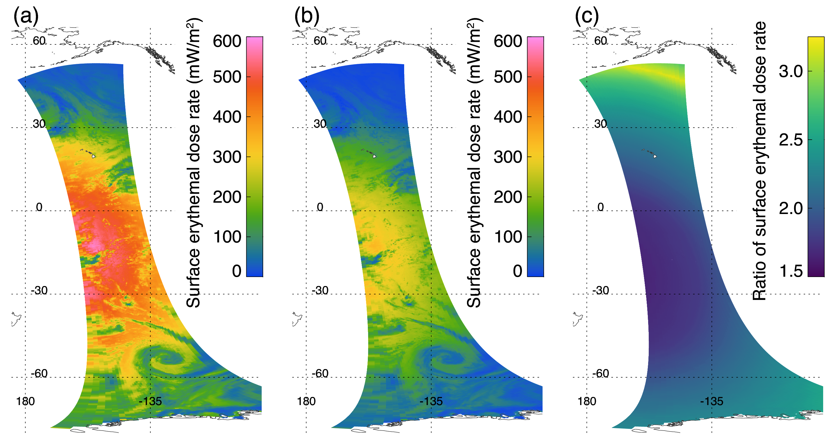
3.1. Surface Irradiance

The Marine Optical Buoy (MOBY) is a facility designed for the vicarious calibration of satellite ocean color instruments [47]. Located in clear ocean waters near the island of Lanai, Hawaii, MOBY measures the upwelling radiance and downwelling irradiance below the ocean surface plus the incident solar irradiance just above the surface. The measurements include a near-UV range down to about 350 nm.
Figure 2 shows the results of comparing the OMI-derived surface irradiance with the MOBY-measured irradiance in the UV. Comparisons were carried out for OMI pixels collocated over the MOBY site. Because the OMI equator crossing time is about 13:45 local time, the MOBY measurements at 14:00 local time are selected to ensure a minimum time difference between the MOBY measurements and OMI overpass time. Only good MOBY measurements under clear skies were used for the comparisons. OMI pixels were collocated for different seasons to encompass the SZA variability over the year 2005. Using the PACE recommended TSIS solar irradiance improved comparisons with MOBY by 2–3%. As can be seen from Figure 2, the computed and measured irradiances agreed rather well; the mean difference was less than 5%.

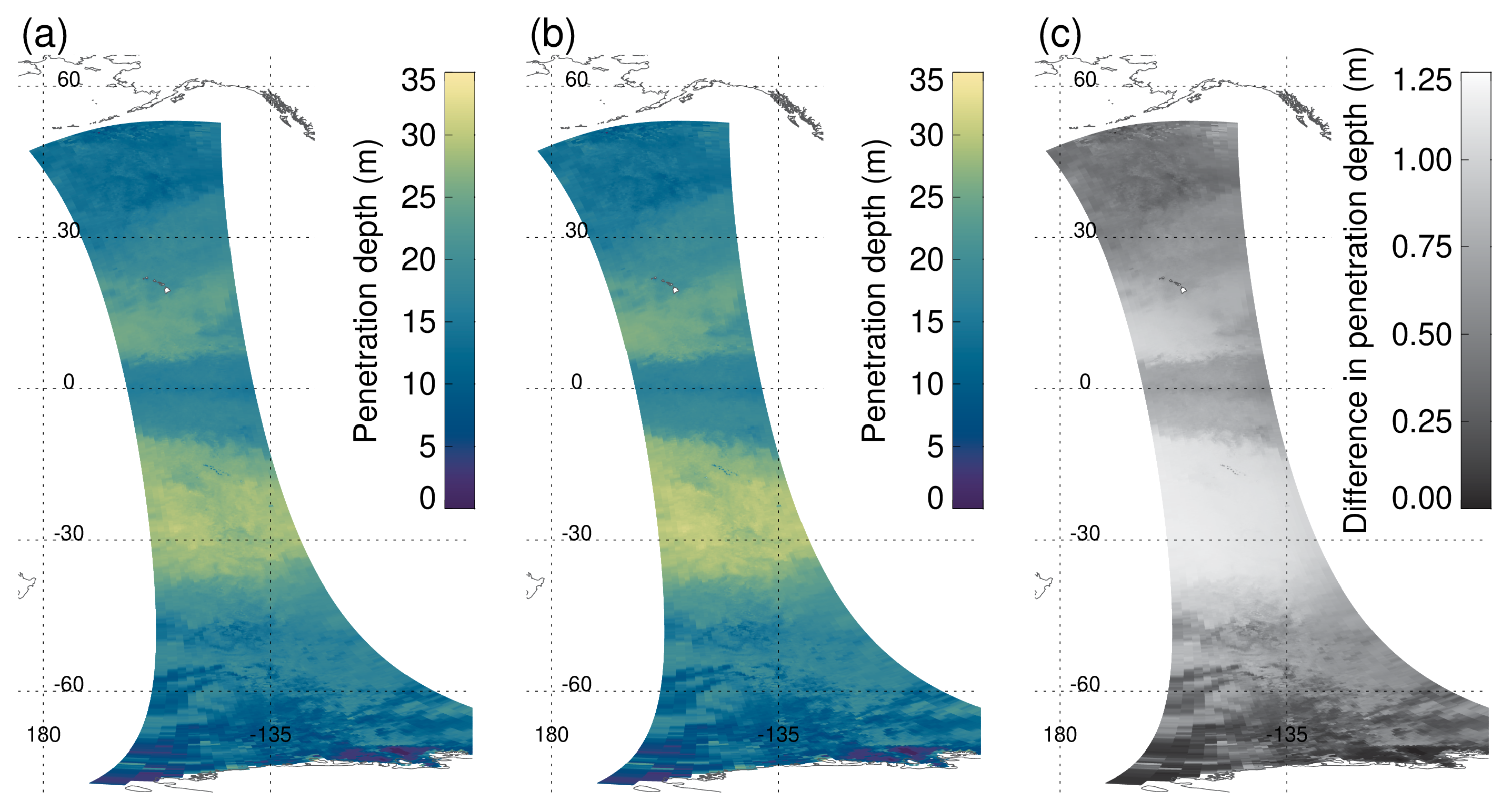
3.2. In-Water Irradiance

We first present the results, which show the main factors affecting the underwater UV radiation field and then the results of the OMI-retrieved characteristics of the radiation field.

3.2.1. Spectral Irradiance

Here, we consider the spectral dependence of planar and scalar irradiances and DNA action-weighted irradiance. The latter is defined as a product of the spectral irradiance and the DNA damage action spectrum [48] (see also https://www.temis.nl/uvradiation/product/action.html, accessed 30 March 2022). Figure 3 shows an example of absolute values of the hyper-spectral planar and scalar irradiances at different depths and the corresponding normalized irradiances along with the DNA action spectrum.
A comparison of the normalized irradiance spectra (Figure 3 right) near the ocean surface and at the depth of 20 m shows how the spectra changed with depth. The most significant reduction of the irradiance occured at shorter wavelengths. As the depth increased, the ocean water mostly cut down the short-wave part of the solar spectrum due to higher absorption at shorter wavelengths.
The DNA-weighted irradiances are shown in Figure 4. It is interesting to note that the spectral maximum of the DNA-weighted irradiances slightly shifted from 303 nm to about 305 nm with depth increasing from 2 m to 20 m. This is explained by the larger absorption of ocean water at shorter wavelengths resulting in the reduction of contribution of shorter wavelengths to the DNA-weighted irradiance. An estimate of the diffuse attenuation coefficient at 305 nm from in situ measurements [49] or satellite observations [16] can provide information on the DNA damage penetration depth.

3.2.2. K-Functions in the UV

In-water attenuation of E d and E o with depth is characterized by the diffuse attenuation coefficient (K-function):
K ( z ) = d ln ( E ) / d z ,
where E is either E d or E o , z is the depth and the wavelength dependence is omitted for briefness. Then, the propagation of E to depth is described by the exponential function:
E ( z ) = E ( 0 ) exp ( 0 z K ( z ) d z ) ,
where E ( 0 ) is the irradiance value at the surface. A penetration depth, z p , can be defined as a depth at which the quantity E decreases to a pre-defined fraction of its surface value ε = E ( z p ) / E ( 0 ) . For instance, in the case that K equals a constant and the commonly used value ε = 0.1 for defining the euphotic zone depth, z 10 % [50], the penetration depth is z p = ln ( 0.1 ) / K .
The diffuse attenuation coefficient at a given depth depends on the angular distribution of radiance and IOPs, e.g., [51]. Here, we compare the diffuse attenuation coefficients for downwelling planar irradiance, K d , and scalar irradiance, K o , as a function of different input variables. Figure 5 shows the dependence of K d and K o on depth, wavelength, chlorophyll concentration and SZA.
The data in Figure 5 show that the dependences of the diffuse attenuation coefficient of scalar and planar irradiance on depth were quite close to each other. Given that the average cosine of the downwelling radiance is defined as μ ( z ) = E d ( z ) / E 0 ( z ) , this means a weak dependence of μ in UV on depth in the upper layer of the ocean due to the following relationship d μ / d z = μ ( K d K o ) . The weak dependence of μ on depth results in a weak dependence of the K functions on depth (see Figure 5b) because we assume a vertically uniform distribution of IOPs. This assumption is well justified for the well-mixed upper layer of the ocean. The weak dependence of the K functions on depth in the upper layer allows for the use of a single value of the K functions averaged over the upper layer for predicting the penetration depths in the UV. This is particularly important for satellite estimates of the diffuse attenuation coefficients [16] because the satellite estimates are based on the measurement of water-leaving radiance, which is primarily formed in the upper layer of the ocean.
The wavelength dependence of the K function shown in Figure 5a was determined by the IOP wavelength dependence. The dominant role in this dependence is played by the spectral dependence of the total absorption coefficient, which significantly increases with decreasing wavelength. Similarly, the dependence of the K functions on chlorophyll (Figure 5c) is explained by the increase in the total absorption coefficient with the increasing chlorophyll concentration (see Appendix A). Figure 5d shows that the K functions increase slightly with increasing SZA. This is explained by the fact that the average cosine of the downwelling radiance decreases due to an increased fraction of the diffuse light in the incident radiation. The dependence of K d and K o on ozone amount is quite small and is not shown in Figure 5.

3.2.3. OMI Retrievals

In this section, OMI retrievals are shown for OMI orbit 2573 on 7 January 2005. All the retrievals are limited to SZA < 80 . The retrievals include the surface erythemal dose rates and penetration depths for the DNA damage dose rates. The DNA damage dose rate at a given depth is defined as the integral of the DNA-weighted irradiance over the UV spectral range:
D ( z ) = 290 400 E ( λ , z , S Z A ) A ( λ ) d λ ,
where E ( λ , z ) is either the planar or scalar irradiance, A ( λ ) is the DNA damage action spectrum [48] and SZA is defined for each OMI pixel at the time of the satellite overpass. The penetration depth is calculated from the following equation: D ( z p ) = ϵ D ( 0 ) , where ε = 0.1 .
Figure 6 shows maps of the main input parameters of orbit 2573 used for the OMI retrievals. The chlorophyll concentrations shown in Figure 6 were obtained from the MODIS/Aqua chlorophyll-a product [52]. We use the monthly averaged Level 3 MODIS chlorophyll product, which is reported at a spatial resolution of 4 km [53]. All available monthly MODIS chlorophyll data within the OMI field-of-view (FOV) were averaged. In the case where MODIS data were not available from the monthly product for an OMI FOV, gap filling was performed using monthly climatology. If monthly data were unavailable, an annual mean was used.
Figure 7 shows maps of the OMI-derived surface erythemal dose rates. The dose rates were calculated using the planar and scalar irradiances convolved with the erythemal action spectrum [54] (see also, https://www.temis.nl/uvradiation/product/action.html, accessed on 30 March 2022).
As expected, the scalar erythemal dose rates were noticeably higher than the planar erythemal dose rates. Both planar-based and scalar-based erythemal dose rates depend on SZA and cloud cover. The erythemal dose rates exhibit a strong spatial correlation with the effective cloud optical depth shown in Figure 6d. The ratio of the scalar dose rates to the planar dose rates (Figure 7c) was highly correlated with SZA (Figure 6a) and increased with SZA except for very high SZA > 70 in the northern part of the orbital swath. For those high SZAs, the ratio decreased with increasing SZA (see Figure A2b of Appendix B). This dependence of the ratio on SZA for high values of SZA was similar to the so-called Umkehr effect that is related to ozone absorption in the atmosphere. In general, the ratio of the scalar erythemal dose rates to the planar erythemal dose rates varied from 1.5 to about 3.0.
Figure 8 shows maps of the penetration depths of the DNA damage dose rates calculated using the planar and scalar irradiance and their difference. The maps of the penetration depths show that a governing parameter that mostly defines the penetration depth is chlorophyll concentration. There is a strong spatial correlation between the chlorophyll concentration (Figure 6b) and the penetration depths (Figure 8a,b). Other input parameters play an insignificant role in the spatial distribution of the penetration depths. The penetration depths vary from a few meters in areas of productive waters of the Southern Ocean to about 30–35 m in the clearest waters of the South Pacific Gyre. Differences between the planar penetration and scalar penetration depths are small. They do not exceed a couple of meters (Figure 8c). This fact follows from Hydrolight computations that show a small difference between K functions for the planar and scalar irradiances for a wide range of input parameters (Figure 5).

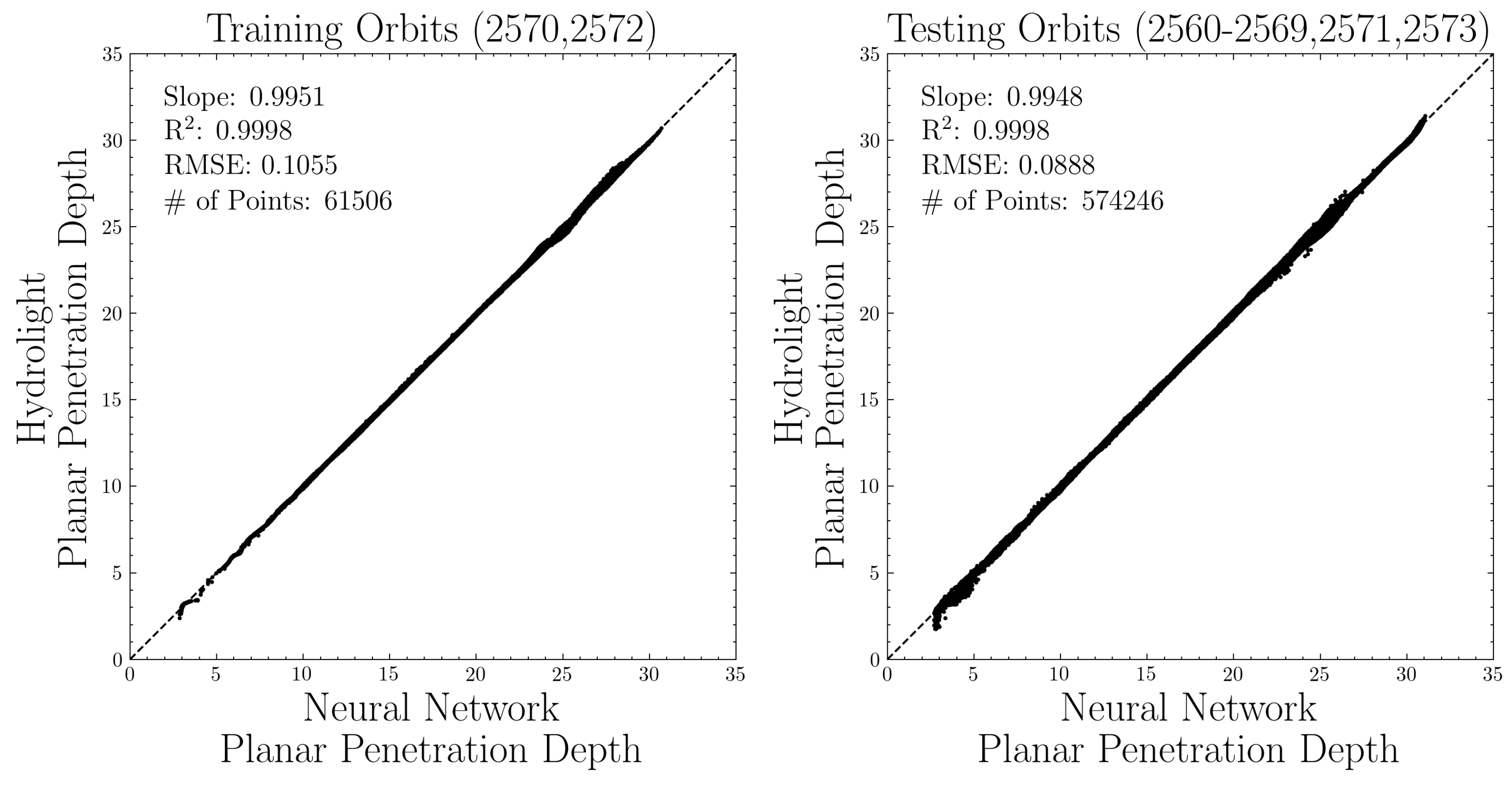
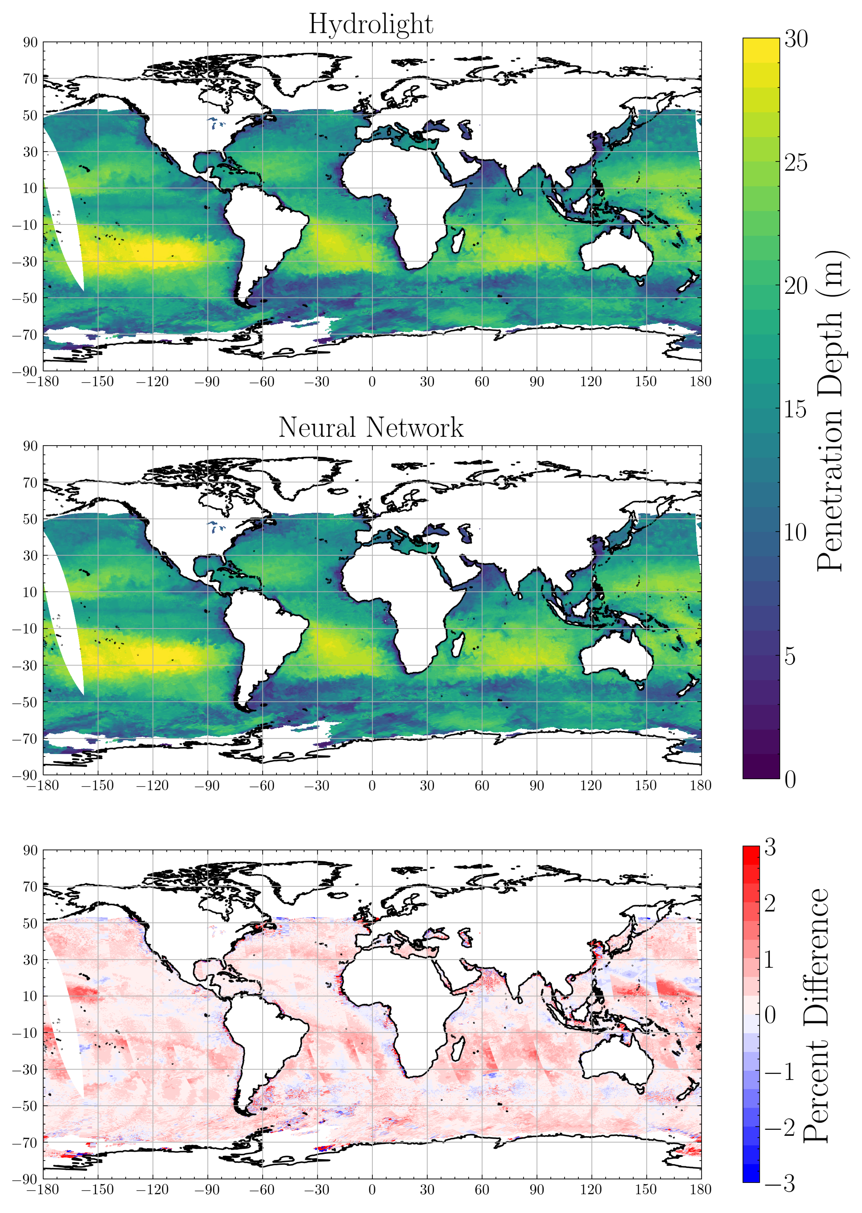
3.3. Machine Learning Results

Forward radiative transfer modeling from tools such as Hydrolight can be computationally inefficient due to the large number of complex non-linear physical equations. The current and future Earth observing satellites continue to provide measurements at higher spectral, spatial and temporal resolutions. As a result of the increased number of measurements, traditional physically based radiative transfer models will not be feasible in operational processing. Machine learning approaches have been proposed to overcome these computational challenges. Machine learning models such as neural networks (NNs) can learn how to represent the complex physical relationships in the radiative transfer simulations through statistical equations [55,56].
Here, we explore the feasibility of using an NN to reproduce the physics-based penetration depth simulations from Hydrolight so that the retrieval algorithm can be applied to an operational sensor such as OMI. The inputs used to estimate penetration depth are SZA, chlorophyll concentration, total column ozone and surface irradiance. For this work, we used a simple four-layer feed-forward neural network with an input layer, two hidden layers and an output layer that predicts planar and scalar penetration depth. The neural network uses a sigmoid activation function for each hidden layer and an adaptive moment estimation optimizer was used to minimize the error with a learning rate of 0.01. We trained the NN with 80% of the samples from two orbits from 7 January 2005 (orbits 2570 and 2572), which include a well-distributed sampling of Case I open waters (low chlorophyll concentration) as well as Case II coastal waters (higher chlorophyll concentration). The neural network was able to predict the penetration depth in approximately two seconds of the computer time for a single orbit as compared with a few minutes of the computer time needed for processing a single orbit by the physics-based algorithm.
Figure 9 shows comparisons of the NN estimates of penetration depth compared to those from the Hydrolight simulations. This figure shows comparisons for orbits included in the training (left panel) as well as additional independent testing orbits not included in the NN training (right panel). There was excellent agreement between the NN results and the Hydrolight simulations with an R 2 of nearly 1 and RMS error of 0.08–0.1 m. The comparisons were quite similar for the training orbits and independent orbits, suggesting that the NN works well for all conditions and is not overfitting to the training samples.
Figure 10 shows maps of the planar penetration depth from Hydrolight (top) and the estimated planar penetration depth from the NN (middle). The NN does well in reproducing the planar penetration depth; differences with Hydrolight were generally < ± 2 % . There were some larger differences off the immediate coast of Antarctica, which are likely due to misclassification of snow or sea ice.

4. Discussion

4.1. IOP Model Limitations

The largest source of uncertainty in the estimation of UV penetration into the ocean is related to the IOP model used in RT computations with Hydrolight. HydroLight is a radiative transfer numerical model that computes radiance distributions and derived quantities for natural water bodies. This model solves the unpolarized RT equation to obtain the radiance distribution within a plane-parallel water body. We neglect the errors of solving the RT equation with Hydrolight because a main source of the errors in the Hydrolight output is related to uncertainties in the Hydrolight input. In general, the Hydrolight inputs consist of the absorbing and scattering properties of water, the properties of the wind-blown ocean surface, the reflectance of the bottom in the case of shallow waters and the angular distribution of radiance incident on the ocean surface.
Here, we assume the Case I model of IOPs that allows us to minimize the number of input parameters and, therefore, to use the standard satellite ocean color product as input for Hydrolight. Within the Case I model, the IOPs of ocean water are assumed to be fully correlated and can be parameterized through chlorophyll concentration. The Case I ocean water model is supposed to work well for open ocean waters where the influence of terrigenic matter is negligible. The Case I model is not applicable for coastal zones of the world ocean where suspended particulate matter and CDOM may not be fully correlated with chlorophyll concentration.
Our parameterization of the particulate-matter absorption coefficient, a p h , Ref. [10] is based on in situ data collected on the California Cooperative Oceanic Fisheries Investigations (CalCOFI) cruises in different areas and seasons. The CalCOFI region encompasses a large dynamic range of coastal and open ocean trophic structures. The optics data have been collected for Chl-a concentrations at the surface, ranging four orders of magnitude, from 0.05 mg m−3 for offshore stations to about 20 mg m−3 and higher. The taxonomic composition across the onshore-offshore gradient ranges from a dinoflagellate/diatom-dominated coastal community to a pico-plankton-dominated community offshore. The offshore region of CalCOFI is typical of the open ocean oligotrophic subtropical gyres with low surface Chl-a and a deep Chl-a maximum between 100–130 m.
Unfortunately, there are few measurements of particulate-matter absorption below 350 nm. That is why a direct comparison of our parameterization with other data is limited. The lack of the a p h ( λ ) data compels us to assume an arbitrary spectral dependence of a p h in the UV. For instance, Westberry et al. [57] assume that a p h is spectrally flat for λ < 412 nm, which is rather unrealistic. However, this model is currently embedded in NASA’s SeaDAS software. A classification of a p h ( λ ) measured down to the 350 nm at 5 nm step was proposed in [58]. The a p h spectra were divided into twelve groups based on a value of a p h ( 440 ) , covering oligotrophic oceanic waters to waters with phytoplankton blooms. However, a parameterization of a p h in UV that would be suitable for a global application was not proposed. Morrison et al. [59] show two normalized phytoplankton absorption spectra from 300 to 750 nm taken at the Bermuda Atlantic Time Series (BATS) site. Their spectra are highly variable with seasons and depths between 300 and 365 nm. This variability is likely due to mycosporine-like amino acids (MAAs), which strongly absorb near 320 nm. The shape of the summer spectrum [59] is quite different from our paramterization. This is explained by averaging many spectra collected in different seasons in our parameterization, while Morrison et al. [59] show examples of the phytoplankton absorption spectra. This discussion suggests the development of a new parameterization based on simultaneous measurements of chlorophyll and MAA concentrations. Hedley and Mobley [60] attempted to combine the data from Vasilkov et al. [10] with the spectra from Morrison et al. [59] in the latest version of Hydrolight. Their attempt gives an absorption model that roughly corresponds to the mid-range of UV absorptions seen in Morrison et al. [59]. We think that this model may be too speculative and do not use it in our computations.
Quantifying the pure water absorption coefficient, a w , is important because there is no consensus on the a w values. There are significant differences between different datasets of a w in the UV. We have discussed the pure water absorption and compared the different datasets in Vasilkov et al. [44,61] (see, e.g., Figure 12 in Vasilkov et al. [61]). The estimates from Vasilkov et al. [61] show that the IOP model could be improved for very low chlorophyll concentrations if we use the data from Lee et al. [62]. However, those data were not derived from direct measurements; they were retrieved from comparisons of the modelled and measured remote sensing reflectances. Moreover, the spectral range of a w data in Lee et al. [62] is not suitable for our purposes because it is limited by the shortest available wavelength (350 nm). That is why we do not use those data.

4.2. Verification of the IOP Model

We have verified the ocean RT and IOP model by comparing the calculated and measured diffuse attenuation coefficients in Vasilkov et al. [10]. Here, we briefly describe the results of the verification. In situ data used in the comparisons are from measurements taken during the Aerosol Characterization Experiment. The (ACE)-Asia experiment was carried out in 2001 in the Pacific Ocean. The dataset includes profile measurements of downward irradiance E d and upward irradiance E u at 17 wavelengths ranging from 313 to 710 nm. In the field measurements of K d , the surface-wave introduced fluctuations in the subsurface light field make it hard to accurately determine K d ( z ) . To compare with the calculated K d , we averaged the measurements over a 10 m layer using linear regression analysis between ln ( E d ( z ) ) and z. Comparisons of the calculated and measured K d , which were completed for chlorophyll concentrations less than 0.7 mg/m3 to ensure the validity of the Case I water model, showed that the correlation coefficient varied from 0.89 at 313, 320 and 340 nm to 0.87 at 380 nm. The relative RMS error for all the cruise stations was less than 20%. There was no obvious bias between the measured and calculated K d , suggesting that the IOP model reasonably reflects the observed absorption and scattering in the ocean. Comparisons between the calculated and measured quantities were also carried out for the diffuse reflectance, R = E u / E d in Vasilkov et al. [44]. The comparisons showed a good agreement between the data: the correlation coefficient varied from 0.85 to 0.90 depending on wavelength.

4.3. Ozone Availability for OCI

Daily column ozone fields are necessary to apply our underwater UV retrieval algorithm to OCI. OMI no longer achieves daily global coverage due to a partial instrument blockage at the Earth-view entrance port. Total column ozone is also available from the series of Ozone Mapping and Profiler Suite (OMPS) nadir mapper (NM) instrument, which will be operating on the Joint Polar Satellite System (JPSS) missions into the next decade. However, it would be preferable for our retrievals to use total ozone produced from the OCI itself. Mannino et al. [63] demonstrated the feasibility of retrieving ozone from PACE, if the UV spectral range of OCI could be extended to bands centered at 322 and 325 nm. They find the quality of retrieved ozone from their approach suitable for the atmospheric correction of ocean color products, and the same is true for underwater UV irradiances.
Another possibility to obtain total column ozone is the use of monthly climatological values. However, some differences between the daily ozone and climatological amounts will inevitably exist. They will lead to errors in the surface and underwater irradiances. For the typical 5 DU (2%) ozone uncertainty, the surface UV uncertainty is 1–3% at 310 nm, increasing to 5–8% at 300 nm and 10–15% at 295 nm. The UV sensitivity to total ozone and its vertical distribution increases for high SZAs and short UVB wavelengths due to the Umkehr effect (see the discussion of Figures 3 and 4 in Krotkov et al. [35]).

5. Conclusions

Scalar irradiance at the ocean surface can be derived from satellite estimates of planar irradiance using the scaling factor from Hydrolight computations. For a clear sky, the scaling factor is a function of wavelength, SZA and ozone amount. The scalar erythemal dose rates calculated at the ocean surface are noticeably higher than the planar erythemal dose rates; their ratio varies from 1.5 to about 3.0. In-water attenuation of E d and E o with depth is quite similar. Differences in the corresponding K-functions are very small for the wide range of input parameters, which include depth, wavelength, SZA, chlorophyll concentration and ozone amount.
A dominant factor defining the UV penetration depths is chlorophyll concentration. Other input parameters play a less significant role in the spatial distribution of the penetration depths. The penetration depths vary from a few meters in areas of productive waters to about 30–35 m in the clearest waters. The machine learning algorithm shows a very good performance with the selected NN architecture in predicting the penetration depths. The NN reproduces the planar penetration depth with errors <± 2 % .

Author Contributions

Conceptualization, A.V. and N.K.; methodology, A.V. and N.K.; software, D.H.; validation, A.V., D.H. and Z.F.; formal analysis, A.V.; investigation, A.V.; resources, Z.F.; data curation, Z.F.; writing—original draft preparation, A.V. and N.K.; writing—review and editing, J.J., D.H. and Z.F.; visualization, A.V. and D.H.; supervision, N.K. and J.J.; project administration, N.K.; funding acquisition, N.K. All authors have read and agreed to the published version of the manuscript.

Funding

This research was funded by NASA through the PACE science team program.

Data Availability Statement

OMI Level 1b UV radiance data are available through NASA’s Goddard Earth Sciences Data and Information Services Center (GES DISC) at https://disc.gsfc.nasa.gov/datasets/OML1BRUG_004/summary. The TSIS-1 HSRS 0.1 nm spectral resolution (“p1nm”) dataset was obtained from the Laboratory for Atmospheric and Space Physics (LASP) at the University of Colorado, Boulder, https://lasp.colorado.edu/lisird/data/tsis1_hsrs. OMI Level 2 total ozone data are available at https://disc.gsfc.nasa.gov/datasetsOMTO3_003/summary. MODIS Level 3 4 km chlorophyll data are available at https://oceancolor.gsfc.nasa.gov/. All accessed on 30 March 2022.

Acknowledgments

We are grateful to the OMI processing team for providing OMI data.

Conflicts of Interest

The authors declare no conflict of interest.

Abbreviations

The following abbreviations are used in this manuscript:
AUAstronomical Unit
BWFBiological Weighting Function
CDOMColored Dissolved Organic Matter
DNADeoxyribonucleic Acid
DUDobson Unit
FOVField of View
IOPInherent Optical Property
MOBYMarine Optical Buoy
MODISModerate Resolution Imaging Spectroradiometer
OCIOcean Color Instrument
OMIOzone Monitoring Instrument
RMSRoot Mean Square
RTRadiative Transfer
SZASolar Zenith Angle
TOATop of the Atmosphere
TSIS-1 HSRSTotal and Spectral Solar Irradiance Sensor Hybrid Solar Reference Spectrum
UVUltraviolet

Appendix A. IOP Model

To carry out RT computations with Hydrolight we need to specify the absorption and scattering coefficients of ocean water along with a phase-scattering function. The total IOPs are built up as a sum of IOPs attributable to the various components of the water body. Thus, the total absorption coefficient is:
a ( λ ) = a w ( λ ) + a p h ( λ ) + a C D O M ( λ ) ,
where a w is the pure ocean water absorption coefficient, a p h is the particulate-matter absorption coefficient and a C D O M is the CDOM absorption coefficient. Similarly, the total scattering coefficient is calculated as follows:
b ( λ ) = b w ( λ ) + b p h ( λ ) ,
where b w is the pure ocean water scattering coefficient, and b p h is the particulate-matter scattering coefficient.
Additionally, we need to specify a phase-scattering function. An intercomparison of different phase scattering functions was carried out in Vasilkov et al. [10] by comparing the calculated K d with the measured K d for different chlorophyll concentrations. Data in this paper show that the physically-based Fournier–Forand (FF) phase function [64] is better in predicting downwelling irradiances than the average Petzold phase function. The FF phase function with a backscatter fraction of 0.003 was used in the computations. This conclusion was confirmed by Vasilkov et al. [44], where comparisons of the calculated diffuse reflectance and measured reflectance were performed.
An important feature of the IOP model in the UV region is quantifying the pure water absorption coefficient, a w . At present, there are significant differences between different datasets of a w in the UV region. A detailed discussion on pure water absorption and comparisons of the different datasets can be found in Vasilkov et al. [44,61]. In this study, we use interpolation between data given in Pope and Fry [65] and Quickenden and Irvin [66], as suggested by Fry [67].
To reduce a number of input parameters to the IOP model, we assume the so-called Case I water model [43,68]. According to this model, all ocean water constituents are of biogenic origin and can be related to a single parameter—chlorophyll concentration. A parameterization of the particulate matter absorption coefficient in the UV as a function of chlorophyll concentration is based on in situ data collected in the framework of the California Cooperative Oceanic Fisheries Investigations (CalCOFI) [10].
The particulate matter absorption coefficient is expressed through a chlorophyll-a concentration and a chlorophyll-specific absorption coefficient similar to that used in the visible part of the spectrum:
a p h ( λ ) = A ( λ ) Chl 1 B ( λ ) ,
where the coefficients A ( λ ) and B ( λ ) are tabulated in [10]. The spectral dependence of a p h and its dependence on chlorophyll concentration are shown in Figure A1 for low chlorophyll concentrations, which are typical for open ocean waters (Case I waters).
Figure A1. The particulate-matter absorption coefficient. Left panel: a p h as a function of wavelength for different chlorophyll concentrations: 1—Chl = 0.55 mg/m3; 2—Chl = 0.13 mg/m3; 3—Chl = 0.03 mg/m3. Right panel: a p h as a function of chlorophyll concentration for different wavelengths: 1–300 nm; 2–340 nm; 3–380 nm.
Remotesensing 14 02278 g0a1
An important absorber in UV is the colored (or chromophoric) dissolved organic matter (CDOM). The spectral CDOM absorption is parameterized in the conventional form:
a C D O M ( λ ) = a C D O M ( λ 0 ) exp [ S ( λ λ 0 ) ] ,
where λ 0 = 440 nm is the reference wavelength, and S is the spectral slope. The CDOM spectral slope typically has somewhat higher values in the UV region as compared with the Vis region. We assume S = 0.017 nm−1, as recommended for the UV [69]. Following Morel and Maritorena [68], the CDOM absorption coefficient at 440 nm is parameterized as:
a C D O M ( 440 ) = 0.2 [ a w ( 440 ) + 0.06 Chl 0.65 ] ,
where a w = 0.0063 m−1 is the pure seawater absorption coefficient [70]. This parameterization assumes that there is some CDOM absorption even in the absence of chlorophyll and models the presence of background CDOM in ocean waters.
The spectral dependence of the particulate matter scattering coefficient is approximated by a power law:
b p ( λ ) = b 0 ( λ / λ 0 ) n ,
where λ 0 = 550 nm is the reference wavelength and the power-law exponent is set to n = 1 [43]. A value of the particulate matter scattering coefficient at the reference wavelength is parameterized through the chlorophyll concentration [68]:
b 0 = 0.416 Chl 0.766
Thus, all the input parameters are functions of only one input quantity—the chlorophyll concentration.

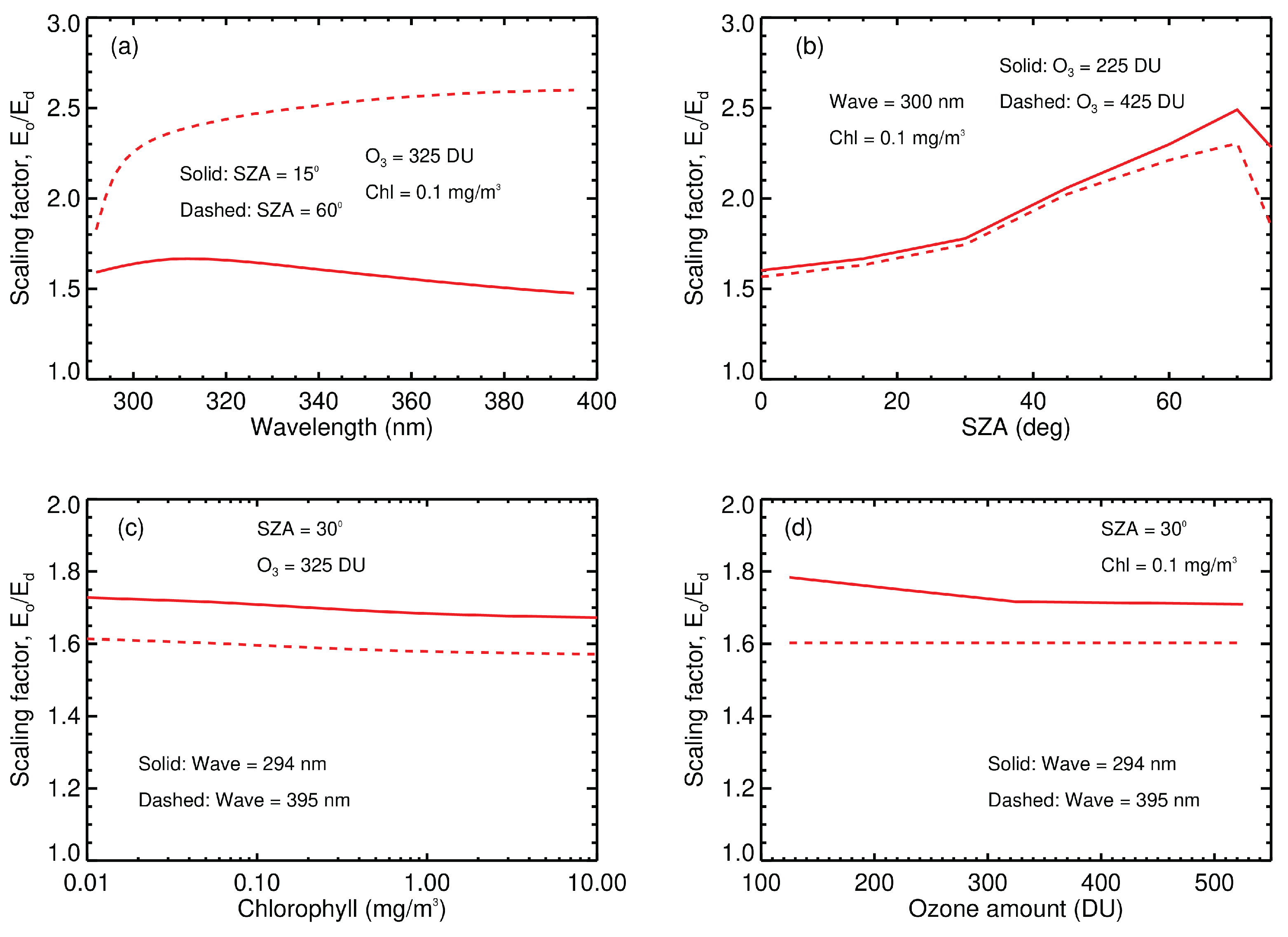
Appendix B. Scaling Factor

The scaling factor f ( λ , SZA , Chl , Ozone ) = E o / E d derived from Hydrolight computations allows us to estimate the scalar irradiance at the ocean surface provided the planar irradiance is known from an external source. In our case, the external source is satellite-derived planar irradiance at the surface. Then we can propagate the scalar irradiance into the ocean body using Hydrolight. The Hydrolight computations are carried out for a specified angular distribution of incoming radiance at the surface, which may differ from the actual angular distribution of incoming radiance. The below results refer to the default boundary conditions of Hydrolight.
Figure A2 shows the scaling factor just above the ocean surface as a function of different input variables.
The most notable dependence of the scaling factor on input parameters is its dependence on SZA (Figure A2b). The scaling factor increases with SZA increasing up to SZA 70 . Then, the scaling factor decreases with increasing SZA. This dependence of the scaling factor on SZA for high values of SZA is similar to the so-called Umkehr effect. Such a dependence of the scaling factor on SZA is explained by a different ozone absorption of the direct and diffuse solar light as a function of SZA in the atmosphere.
Figure A2. The scaling factor dependence on different variables; (a) the f dependence on wavelength for different SZAs; (b) the f dependence on SZA at 300 nm for different ozone amounts; (c) the f dependence on chlorophyll concentration for different wavelengths. (d) The f dependence on ozone amount for different wavelengths.
Remotesensing 14 02278 g0a2

References

  1. Häder, D.-P.; Williamson, C.E.; Wängberg, S.-A.; Rautio, M.; Rose, K.C.; Gao, K.; Helbling, E.W.; Sinhahand, R.P.; Worrest, R. Effects of UV radiation on aquatic ecosystems and interactions with other environmental factors. Photochem. Photobiol. Sci. 2015, 14, 108–126. [Google Scholar] [CrossRef] [PubMed] [Green Version]
  2. Litchman, E.; Neale, P.J. UV effects on photosynthesis, growth and acclimation of an estuarine diatom and cryptomonad. Mar. Ecol. Prog. Ser. 2005, 100, 53–62. [Google Scholar] [CrossRef]
  3. Cullen, J.J.; Neale, P.J.; Lesser, M.P. Biological weighting function for the inhibition of phytoplankton photosynthesis by ultraviolet radiation. Science 1992, 258, 646–650. [Google Scholar] [CrossRef] [PubMed]
  4. Boucher, N.P.; Prezelin, B.B. An in situ biological weighting function for UV inhibition of phytoplankton carbon fixation in the Southern Ocean. Mar. Ecol. Prog. Ser. 1996, 144, 223–236. [Google Scholar] [CrossRef]
  5. Neale, P.J.; Pritchard, A.L.; Ihnacik, R. UV effects on the primary productivity of picophytoplankton: Biological weighting functions and exposure response curves of Synechococcus. Biogeosciences 2014, 11, 2883–2895. [Google Scholar] [CrossRef] [Green Version]
  6. Bélanger, S.; Xie, H.; Krotkov, N.; Larouche, P.; Vincent, W.F.; Babin, M. Photomineralization of terrigenous dissolved organic matter in Arctic coastal waters from 1979 to 2003: Interannual variability and implications of climate change. Global Biogeochem. Cycles 2006, 20, GB4005. [Google Scholar] [CrossRef]
  7. Moran, M.A.; Zepp, E.G. Role of photoreactions in the formation of biologically labile compounds from dissolved organic matter. Limnol. Oceanogr. 1997, 42, 1307–1316. [Google Scholar] [CrossRef] [Green Version]
  8. Vasilkov, A.P.; Krotkov, N.A. Modeling the effect of seawater optical properties on the ultraviolet radiant fluxes in the ocean. Izv. Atmos. Ocean. Phys. 1997, 33, 349–357. [Google Scholar]
  9. Vasilkov, A.P.; Krotkov, N.; Herman, J.R.; McClain, C.; Arrigo, K.; Robinson, W. Global mapping of underwater UV irradiance and DNA-weighted exposures using TOMS and SeaWiFS data products. J. Geophys. Res. 2001, 106, 27205–27219. [Google Scholar] [CrossRef]
  10. Vasilkov, A.; Herman, J.; Ahmad, Z.; Kahru, M.; Mitchell, B.G. Assessment of the ultraviolet radiation field in ocean waters from space-based measurements and full radiative-transfer calculations. Appl. Opt. 2005, 44, 2863–2869. [Google Scholar] [CrossRef]
  11. Mobley, C.D. Light and Water: Radiative Transfer in Natural Waters; Academic Press: Cambridge, MA, USA, 1994; 592p. [Google Scholar]
  12. Ahmad, Z.; Herman, J.R.; Vasilkov, A.; Tzortziou, M.; Mitchell, G.; Kahru, M. Seasonal variation of UV radiation in the ocean under clear and cloudy conditions. In Ultraviolet Ground-and Space-Based Measurements, Models, and Effects III; Slusser, J.R., Herman, J.R., Gao, W., Eds.; SPIE: Bellingham, WA, USA, 2003; pp. 63–73. [Google Scholar]
  13. Fichot, C.G.; Sathyendranath, S.; Miller, W.L. SeaUV and SeaUVC: Algorithms for the retrieval of UV/visible diffuse attenuation coefficients from ocean color. Remote Sens. Environ. 2008, 112, 1584–1602. [Google Scholar] [CrossRef]
  14. Smyth, T.J. Penetration of UV irradiance into the global ocean. J. Geophys. Res. 2011, 116. [Google Scholar] [CrossRef]
  15. Lee, Z.; Hu, C.; Shang, A.; Du, K.; Lewis, M.; Arnone, R.; Brewin, R. Penetration of UV-visible solar radiation in the global oceans: Insights from ocean color remote sensing. J. Geophys. Res. Oceans 2013, 118, 4241–4255. [Google Scholar] [CrossRef] [Green Version]
  16. Wang, Y.; Lee, Z.; Ondrusek, M.; Li, X.; Zhang, S.; Wu, J. An evaluation of remote sensing algorithms for the estimation of diffuse attenuation coefficients in the ultraviolet bands. Opt. Express 2022, 30, 6640–6655. [Google Scholar] [CrossRef] [PubMed]
  17. Dinter, T.; Rozanov, V.V.; Burrows, J.P.; Bracher, A. Retrieving the availability of light in the ocean utilising spectral signatures of vibrational Raman scattering in hyper-spectral satellite measurements. Ocean Sci. 2015, 11, 373–389. [Google Scholar] [CrossRef] [Green Version]
  18. Oelker, J.; Richter, A.; Dinter, T.; Rozanov, V.V.; Burrows, J.P.; Bracher, A. Global diffuse attenuation derived from vibrational raman scattering detected in hyperspectral backscattered satellite spectra. Opt. Express 2019, 27, A829–A855. [Google Scholar] [CrossRef]
  19. Oelker, J.; Losa, S.N.; Richter, A.; Bracher, A. TROPOMI-Retrieved underwater light attenuation in three spectral regions in the ultraviolet and blue. Front. Mar. Sci. 2022, 9, 296. [Google Scholar] [CrossRef]
  20. Frouin, R.; Ramon, D.; Boss, E.; Jolivet, D.; Compiègne, M.; Tan, J.; Bouman, H.; Jackson, T.; Franz, B.; Platt, T.; et al. Satellite radiation products for ocean biology and biogeochemistry: Needs, State-of-the-Art, Gaps, Development Priorities, and Opportunities. Front. Mar. Sci. 2018, 5, 3. [Google Scholar] [CrossRef] [Green Version]
  21. Cetinić, I.; McClain, C.R.; Werdell, P.J. (Eds.) PreAerosol, Clouds, and ocean Ecosystem (PACE) Mission Science Definition Team Report; PACE Tech. Rep. NASA/TM2018-219027; NASA: Greenbelt, MD, USA, 2018; Volume 2, p. 316. [Google Scholar]
  22. Tanskanen, A.; Krotkov, N.; Herman, J.R.; Bhartia, P.K.; Arola, A. Surface UV irradiance from OMI. IEEE Trans. Geosci. Remote Sens. 2006, 44, 1267–1271. [Google Scholar] [CrossRef]
  23. Coddington, O.M.; Richard, E.C.; Harber, D.; Pilewskie, P.; Woods, T.N.; Chance, K.; Liu, X.; Sun, K. The TSIS-1 Hybrid Solar Reference Spectrum. Geophys. Res. Lett. 2021, 48, e2020GL091709. [Google Scholar] [CrossRef]
  24. Richard, E.; Harber, D.; Coddington, O.; Drake, G.; Rutkowski, J.; Triplett, M.; Pilewskie, P.; Woods, T. SI-traceable spectral irradiance radiometric characterization and absolute calibration of the TSIS-1 Spectral Irradiance Monitor (SIM). Remote Sens. 2020, 12, 1818. [Google Scholar] [CrossRef]
  25. Levelt, P.F.; Joiner, J.; Tamminen, J.; Veefkind, J.P.; Bhartia, P.K.; Stein Zweers, D.C.; Duncan, B.N.; Streets, D.G.; Eskes, H.; van der, A.R.; et al. The Ozone Monitoring Instrument: Overview of 14 years in space. Atmos. Chem. Phys. 2018, 18, 5699–5745. [Google Scholar] [CrossRef] [Green Version]
  26. Levelt, P.F.; van den Oord, G.H.J.; Dobber, M.R.; Mälkki, A.; Visser, H.; de Vries, J.; Stammes, P.; Lundell, J.; Saari, H. The Ozone Monitoring Instrument. IEEE Trans. Geosci. Remote 2006, 44, 1093–1101. [Google Scholar] [CrossRef]
  27. Dobber, M.R. OMI/Aura Level 1B UV Global Geolocated Earthshine Radiances (V003) [Dataset], Goddard Earth Sciences Data and Information Services Center (GES DISC). 2007. Available online: https://disc.gsfc.nasa.gov/datasets/OML1BRUG_003/summary (accessed on 30 March 2022).
  28. Dobber, M.R. OMI/Aura Level 1B IRR Solar Irradiances (V003) [Dataset], Goddard Earth Sciences Data and Information Services Center (GES DISC). 2007. Available online: https://disc.gsfc.nasa.gov/datasets/OML1BIRR_003/summary (accessed on 30 March 2022).
  29. Schenkeveld, V.M.E.; Jaross, G.; Marchenko, S.; Haffner, D.; Kleipool, Q.L.; Rozemeijer, N.C.; Veefkind, J.P.; Levelt, P.F. In-flight performance of the Ozone Monitoring Instrument. Atmos. Meas. Tech. 2017, 10, 1957–1986. [Google Scholar] [CrossRef] [PubMed] [Green Version]
  30. Balis, D.; Kroon, M.; Koukouli, M.E.; Brinksma, E.J.; Labow, G.; Veefkind, J.P.; McPeters, R.D. Validation of Ozone Monitoring Instrument total ozone column measurements using Brewer and Dobson spectrophotometer ground-based observations. J. Geophys. Res. 2007, 112. [Google Scholar] [CrossRef] [Green Version]
  31. Bhartia, P.K. OMI/Aura Ozone (O3) Total Column 1-Orbit L2 Swath 13 × 24 km V003, Greenbelt, MD, USA, Goddard Earth Sciences Data and Information Services Center (GES DISC). 2005. Available online: https://disc.gsfc.nasa.gov/datasets/OMTO3_003/summary (accessed on 30 March 2022).
  32. Kleipool, Q.L.; Dobber, M.R.; de Haan, J.F.; Levelt, P.F. Earth surface reflectance climatology from 3 years of OMI data. J. Geophys. Res. 2008, 113, D18308. [Google Scholar] [CrossRef]
  33. Kleipool, Q.L. OMI/Aura Surface Reflectance Climatology L3 Global Gridded 0.5 degree x 0.5 degree V3, Greenbelt, MD, USA, Goddard Earth Sciences Data and Information Services Center (GES DISC). 2010. Available online: https://disc.gsfc.nasa.gov/datasets/OMLER_003/summary (accessed on 30 March 2022).
  34. Zhai, P.; Hu, Y.; Chowdhary, J.; Trepte, C.R.; Lucker, P.L.; Josset, D.B. A vector radiative transfer model for coupled atmosphere and ocean systems with a rough interface. J. Quant. Spectr. Radiat. Trans. 2010, 111, 1025–1040. [Google Scholar] [CrossRef]
  35. Krotkov, N.A.; Bhartia, P.K.; Herman, J.R.; Fioletov, V.; Kerr, J. Satellite estimation of spectral surface UV irradiance in the presence of tropospheric aerosols 1. Cloud-free case. J. Geophys. Res. 1998, 103, 8779–8794. [Google Scholar] [CrossRef] [Green Version]
  36. Krotkov, N.A.; Herman, J.R.; Bhartia, P.K.; Fioletov, V.; Ahmad, Z. Satellite estimation of spectral surface UV irradiance 2. Effects of homogeneous clouds and snow. J. Geophys. Res. 2001, 106, 11743–11760. [Google Scholar] [CrossRef]
  37. Deirmendjian, D. Electromagnetic Scattering on Spherical Polydispersions; Elsevier: New York, NY, USA, 1969; 290p. [Google Scholar]
  38. Joiner, J.; Vasilkov, A.P.; Flittner, D.E.; Gleason, J.F.; Bhartia, P.K. Retrieval of cloud pressure and oceanic chlorophyll content using Raman scattering in GOME ultraviolet spectra. J. Geophys. Res. 2004, 109, D01109. [Google Scholar] [CrossRef]
  39. Stamnes, K.; Tsay, S.C.; Wiscombe, W.; Jayaweera, K. Numerically stable algorithm for discrete-ordinate-method radiative transfer in multiple scattering and emitting layered media. Appl. Opt. 1988, 27, 2502–2509. [Google Scholar] [CrossRef] [PubMed]
  40. Ahmad, Z.; Fraser, R. An iterative radiative transfer code for ocean-atmosphere systems. J. Atrnos. Sci. 1982, 39, 656–665. [Google Scholar] [CrossRef] [Green Version]
  41. Krotkov, N.A.; Herman, J.R.; Bhartia, P.K.; Seftor, C.; Arola, A.; Kaurola, J.; Taalas, P.; Vasilkov, A.P. OMI Surface UV Irradiance Algorithm. OMI Algorithm Theoretical Basis Document. Clouds, Aerosols, and Surface UV Irradiance. Available online: http://eospso.gsfc.nasa.gov/sites/default/files/atbd/ATBD-OMI-03.pdf (accessed on 30 March 2022).
  42. Frouin, R.; Tan, J.; Ramon, D.; Franz, B.; Murakami, H. Estimating photosynthetically available radiation at the ocean surface from EPIC/DSCOVR data. In Remote Sensing of the Open and Coastal Ocean and Inland Waters; International Society for Optics and Photonics: Bellingham, WA, USA, 2018; Volume 10778, p. 1077806. [Google Scholar]
  43. Morel, A. Optical modeling of the upper ocean in relation to its biogeneous matter content (Case I waters). J. Geophys. Res. 1988, 93, 10749–10768. [Google Scholar] [CrossRef] [Green Version]
  44. Vasilkov, A.; Lyapustin, A.; Mitchell, B.G.; Huang, D. UV Reflectance of the Ocean from DSCOVR/EPIC: Comparisons with a Theoretical Model and Aura/OMI Observations. J. Atmos. Oceanic Tech. 2019, 36, 2087–2099. [Google Scholar] [CrossRef]
  45. Vasilkov, A.P.; Joiner, J.; Gleason, J.; Bhartia, P.K. Ocean Raman scattering in satellite backscatter UV measurements. Geophys. Res. Lett. 2002, 29, 14–18. [Google Scholar] [CrossRef] [Green Version]
  46. Liu, C.-C.; Carder, K.L.; Miller, R.L.; Ivey, J.E. Fast and accurate model of underwater scalar irradiance. Appl. Opt. 2002, 41, 4962–4974. [Google Scholar] [CrossRef]
  47. Clark, D.K.; Feinholz, M.E.; Yarbrough, M.A.; Johnson, B.C.; Brown, S.W.; Kim, Y.S.; Barnes, R.A. Overview of the radiometric calibration of MOBY. In Earth Observing Systems VI; International Society for Optics and Photonics: Bellingham, WA, USA, 2002; Volume 4483, pp. 64–76. [Google Scholar]
  48. Setlow, R.B. The wavelengths in sunlight effective in producing skin cancer: A theoretical analysis. Proc. Natl. Acad. Sci. USA 1974, 71, 3363–3366. [Google Scholar] [CrossRef] [Green Version]
  49. Tedetti, M.; Sempere, R.; Vasilkov, A.; Charriere, B.; Nerini, D.; Miller, W.L.; Kawamura, K.; Raimbault, P. High penetration of ultraviolet radiation in the south east Pacific waters. Geophys. Reas. Lett. 2007, 34, L12610. [Google Scholar] [CrossRef] [Green Version]
  50. Lee, Z.; Weidemann, A.; Kindle, J.; Arnone, R.; Carder, K.L.; Davis, C. Euphotic zone depth: Its derivation and implication to ocean-color remote sensing. J. Geophys. Res. 2007, 112, C03009. [Google Scholar] [CrossRef] [Green Version]
  51. Lee, Z.-P.; Du, K.-P.; Arnone, R. A model for the diffuse attenuation coefficient of downwelling irradiance. J. Geophys. Res. 2005, 110, C02016. [Google Scholar] [CrossRef]
  52. Hu, C.; Lee, Z.; Franz, B.A. Chlorophyll-a algorithms for oligotrophic oceans: A novel approach based on three-band reflectance difference. J. Geophys. Res. 2012, 117, C01011. [Google Scholar] [CrossRef] [Green Version]
  53. NASA Goddard Space Flight Center, Ocean Ecology Laboratory, Ocean Biology Processing Group. Moderate-Resolution Imaging Spectroradiometer (MODIS) Aqua Chlorophyll Data; 2018 Reprocessing; NASA OB.DAAC: Greenbelt, MD, USA, 2018. [Google Scholar] [CrossRef]
  54. McKinlay, A.; Diffey, B. A reference action spectrum for ultraviolet induced erythema in human skin. CIE J. 1987, 6, 17–22. [Google Scholar]
  55. Fan, Y.; Li, W.; Chen, N.; Ahn, J.-H.; Park, Y.-J.; Kratzer, S.; Schroeder, T.; Ishizaka, J.; Chang, R.; Stamnes, K. A machine learning based data analysis platform for satellite ocean color sensors. Remote Sens. Environ. 2021, 253, 112236. [Google Scholar] [CrossRef]
  56. Fasnacht, Z.; Joiner, J.; Haffner, D.; Qin, W.; Vasilkov, A.; Castellanos, P.; Krotkov, N. Using machine learning for timely estimates of ocean color information from hyperspectral satellite measurements in the presence of clouds, aerosols, and sunglint. Front. Remote Sens. 2022, 2, 34. [Google Scholar] [CrossRef]
  57. Westberry, T.K.; Boss, E.; Lee, Z. Influence of Raman scattering on ocean color inversion models. Appl. Opt. 2013, 52, 5552–5561. [Google Scholar] [CrossRef]
  58. Chowdhary, J.; Zhai, P.-W.; Boss, E.; Dierssen, H.; Frouin, R.; Ibrahim, A.; Lee, Z.; Remer, L.A.; Twardowski, M.; Xu, F.; et al. Modeling atmosphere-ocean radiative transfer: A PACE mission perspective. Front. Earth Sci. 2019, 7, 100. [Google Scholar] [CrossRef]
  59. Morrison, J.R.; Nelson, N.B. Seasonal cycle of phytoplankton UV absorption at the Bermuda Atlantic Time-series Study (BATS) site. Limnol. Oceanogr. 2004, 49, 215–224. [Google Scholar] [CrossRef]
  60. Hedley, J.D.; Mobley, C.D. HYDROLIGHT 6.0 ECOLIGHT 6.0 Technical Documentation; Numerical Optics Ltd.: Tiverton, UK, 2019. [Google Scholar]
  61. Vasilkov, A.; Herman, J.; Krotkov, N.A.; Kahru, M.; Mitchell, B.G.; Hsu, C. Problems in assessment of the ultraviolet penetration into natural waters from space-based measurements. Opt. Eng. 2002, 41, 3019–3027. [Google Scholar] [CrossRef]
  62. Lee, Z.; Wei, J.; Voss, K.; Lewis, M.; Bricaud, A.; Huot, Y. Hyperspectral absorption coefficient of ‘‘pure’’ seawater in the range of 350–550 nm inverted from remote sensing reflectance. Appl. Opt. 2015, 54, 546–558. [Google Scholar] [CrossRef]
  63. Mannino, A.; Haffner, D.; Robinson, W.; Ahmad, Z. Extended UV Capability on OCI for Ozone Retrieval, in PACE Technical Report Series: Ocean Color Instrument (OCI) Concept Design Studies (NASA/TM-2018-2018–219027-); Cetinić, I., McClain, C.R., Werdell, P.J., Eds.; NASA Goddard Space Flight Space Center Greenbelt: Prince George’s County, MD, USA, 2018; Volume 7. [Google Scholar]
  64. Fournier, G.; Forand, J.L. Analytic phase functions for ocean water. Proc. SPIE 1994, 2258, 194–201. [Google Scholar]
  65. Pope, R.M.; Fry, E.S. Absorption spectrum (380–700 nm) of pure water. II. Integrating cavity measurements. Appl. Opt. 1997, 36, 8710–8723. [Google Scholar] [CrossRef] [PubMed]
  66. Quickenden, T.I.; Irvin, J.A. The ultraviolet absorption spectrum of liquid water. J. Chem. Phys. 1980, 72, 4416–4428. [Google Scholar] [CrossRef]
  67. Fry, E.S. Visible and near ultraviolet absorption spectrum of liquid water. Appl. Opt. 2000, 39, 2743–2744. [Google Scholar] [CrossRef] [PubMed]
  68. Morel, A.; Maritorena, S. Bio-optical properties of oceanic waters: A reappraisal. J. Geophys. Res. 2001, 106, 7163–7180. [Google Scholar] [CrossRef] [Green Version]
  69. Kopelevich, O.V.; Lutsarev, S.V.; Rodionov, V.V. Light spectral absorption by yellow substance of ocean water. Oceanology 1989, 29, 409–414. [Google Scholar]
  70. Morel, A.; Gentili, B.; Claustre, H.; Babin, M.; Bricaud, A.; Ras, J.; Tieche, F. Optical properties of the ‘‘clearest’’ natural waters. Limnol. Oceanogr. 2007, 52, 217–229. [Google Scholar] [CrossRef]
Figure 1. Extraterrestrial spectral irradiance at different spectral resolutions shown for (a) the entire UV spectral range and (b) the OCI spectral range shown in the light blue cutout in (a). The color bar represents the boxcar smoothing width in nanometers.
Remotesensing 14 02278 g001
Figure 2. (a) A comparison of the smoothed E s measurements from MOBY (solid line) and OMI (symbols) using the Solar Ultraviolet Spectral Irradiance Monitor (plus signs) and TSIS (asterisks) extraterrestrial solar irradiance spectra for a selected OMI pixel. (b) The mean difference and standard deviation between the OMI-derived surface irradiance and the MOBY-measured irradiance.
Remotesensing 14 02278 g002
Figure 3. Spectral planar (solid lines) and scalar (dashed lines) irradiances. Left: Absolute values of the irradiances at two depths: 2 m (red lines) and 20 m (blue lines). Right: Planar and scalar irradiances normalized over their values at 400 nm. The black line shows the DNA damage action spectrum.
Remotesensing 14 02278 g003
Figure 4. DNA-weighted planar (solid lines) and scalar (dashed lines) irradiances at two depths: 2 m (red lines) and 20 m (blue lines).
Remotesensing 14 02278 g004
Figure 5. Diffuse attenuation coefficient K d (red lines) and K o (blue lines) as a function of: (a) wavelength, (b) depth for two SZAs of 15 (solid lines) and 60 (dashed lines), (c) chlorophyll concentration for two wavelengths 300 nm (solid lines) and 380 nm (dashed lines) and (d) SZA for two values of chlorophyll concentration 0.1 mg/m3 (solid lines) and 1.0 mg/m3 (dashed lines).
Remotesensing 14 02278 g005
Figure 6. Maps of the main input parameters: (a) solar zenith angle; (b) chlorophyll concentration in mg/m3; (c) ozone amounts in DU; and (d) effective cloud optical depth at 360 nm.
Remotesensing 14 02278 g006
Figure 7. Maps of the surface erythemal dose rates: (a) calculated using the scalar irradiance; (b) calculated using the planar irradiance; (c) ratio of the scalar erythemal dose rate to the planar dose rate.
Remotesensing 14 02278 g007
Figure 8. Maps of the penetration depths for the DNA damage dose rates: (a) calculated using the planar irradiance; (b) calculated using the scalar irradiance. (c) The difference between the planar penetration and scalar penetration depths. The color bars represent the penetration depths in meters.
Remotesensing 14 02278 g008
Figure 9. Comparisons of Hydrolight penetration depth simulations and neural network estimate for 7 January 2005. Left panel shows comparisons for orbits included in neural network training while right panel shows orbits on this date not included in the training.
Remotesensing 14 02278 g009
Figure 10. Map of planar penetration depth on 7 January 2005. Top panel shows planar penetration depth from Hydrolight, middle panel shows planar penetration depth from the neural network and the bottom shows the percent difference of Hydrolight versus the neural network estimate. The color bars represent the penetration depths in meters and the percent difference.
Remotesensing 14 02278 g010
Publisher’s Note: MDPI stays neutral with regard to jurisdictional claims in published maps and institutional affiliations.

