Article

Comparison of the Spatial and Temporal Variability of Cloud Amounts over China Derived from Different Satellite Datasets

1
International Center for Climate and Environment Sciences, Institute of Atmospheric Physics, Chinese Academy of Sciences, Beijing 100029, China
2
College of Earth and Planetary Sciences, University of Chinese Academy of Sciences, Beijing 100049, China
3
Collaborative Innovation Center on Forecast and Evaluation of Meteorological Disasters, Nanjing University of Information Science and Technology, Nanjing 210044, China
*
Author to whom correspondence should be addressed.
Remote Sens. 2022, 14(9), 2173; https://doi.org/10.3390/rs14092173
Submission received: 31 March 2022 / Revised: 22 April 2022 / Accepted: 27 April 2022 / Published: 30 April 2022
(This article belongs to the Section Atmospheric Remote Sensing)

Abstract

:
Various cloud cover products have been developed over the past few decades, but their uncertainties have not been sufficiently assessed, especially at a regional scale, which is vital for the application of satellite products to climate studies. In this study, we compare the spatial–temporal variability of the cloud amount over China from the 11 datasets provided by the Global Energy and Water Cycle Experiment (GEWEX) cloud assessment project at a horizontal resolution of 1° × 1° from the 1980s to 2000s, using the site data as a reference. The differences among these datasets are quantified in terms of the standard deviations and the correlation coefficients between different datasets. Most of the datasets show a similar spatial distribution of total cloud amounts (TCAs), but their magnitudes differ. The standard deviations of the annual, winter, and summer mean TCA are approximately 9–18% for the regional mean TCAs over the four typical regions of China, including the northwestern region (NW), northeastern region (NE), Tibetan Plateau region (TP), and southern China region (SC), with the largest standard deviations of 13–18% in the TP. By analyzing the factors that influence the satellite inversion data, such as the observation instrument, inversion algorithm, and observation time, we found that the difference caused by the observation instrument or algorithm is greater than the effect of the observation time, and the satellite cloud datasets with better recognition capability for cloud types show lower uncertainties when compared with the station observation. In terms of seasonal cycle, except HIRS and MODIS-ST, most satellite datasets can reproduce the observed seasonal cycle with the largest TCA in summer and the smallest TCA in autumn and winter. For the interannual variation, ISCCP-D1, MODIS-CE, and MODIS-ST are most consistent with the site data for the annual mean TCA, and two of the remaining datasets (PATMOSX and TOVSB) show more consistent temporal variations with the site observation in summer than in winter, especially over NW and NE regions. In general, MODIS-CE shows the best performance in reproducing the spatial pattern and interannual variation of TCA amongst the 11 satellite datasets, and PATMOSX, MODIS-ST, CALIPSO-GOCCP, and CALIPSO-ST also show relatively good performance.

Graphical Abstract

1. Introduction

Clouds play a significant role in Earth’s energy and water cycles. Approximately 2/3 of the global area is covered by clouds. Clouds greatly impact the Earth’s radiation budget by reflecting the sun’s shortwave radiation back into space and absorbing and reemitting longwave radiation back into the atmosphere [1,2]. Clouds also regulate the atmospheric hydrological cycle by transporting water away from Earth’s surface and redistributing it through precipitation [3].
In climate models, cloud amount is one of the key parameters in the calculation of cloud radiation–precipitation interactions [4,5]. To understand current climate changes and predict future climatic variability, observationally based cloud fraction estimates have been intensively studied for decades. Evidence of climate change has been identified in satellite cloud records. For example, Norris et al. [6] found large-scale changes in the cloud amount between the 1980s and 2000s using several independent and empirically corrected satellite records, which are similar to those produced by climate models with recent historical external radiative forcings. Ding et al. [7] used International Satellite Cloud Climatology Project (ISCCP) data to analyze the total cloud amount (TCA) changes over the past 20 years and their possible climatological impact, and they concluded that TCA changes may initialize a positive feedback process in the climate system; the decreasing TCA observed in recent years may cause the global climate to become warmer. In addition, cloud products retrieved from observations have also been widely used in evaluating model performance. Ban-Weiss et al. [8] evaluated clouds, aerosols, and their interactions in three global climate models using Moderate Resolution Imaging Spectroradiometer (MODIS) satellite observations. Lacagnina and Selten [9] used ISCCP data to assess clouds and radiative fluxes in the EC-Earth general circulation model and found a large cloud amount bias in the tropics. Jin et al. [10] compared ISCCP-simulated data from the Coupled Model Intercomparison Project Phase 5 (CMIP5) models with the corresponding ISCCP observations based on the concept of cloud regimes. The results show that the model-simulated clouds tended to optically be too thick and not as extensive as the observed clouds. Dolinar et al. [11] evaluated CMIP5-simulated clouds and top of the atmosphere (TOA) radiation budgets using CERES, MODIS, ISCCP, CloudSat, and CALIPSO. The results show that the multi-model ensemble mean cloud fraction is underestimated compared to all of the satellite datasets. It is also found that cloud amount is a primary modulator of warming (or cooling) in the atmosphere. Compared with the CMIP5 model, the CMIP6 climate model has improved cloud parameterization processes [12]. However, there is still a large deviation in the simulation of the clouds and their radiation effect [13].
Satellites are the only tools that document clouds at the global scale, but the definition of a cloud depends on the cloud algorithm used and is not unique to different satellite observations. The satellite-retrieved cloud data used to build the cloud climatology datasets are affected by the type of instrument (passive, active), wavelength of the instrument, sensitivity of the sensors, threshold of detection, and spatiotemporal sampling resolution [14], which might lead to inconsistencies between different satellite cloud products. For example, MODIS observes less mid-level cloud than the ISCCP [15]. High thin clouds are not observable in the conventional ISCCP dataset, but can be detected by CALIPSO observations [16]. Marchand et al. [17] also found notable differences in the joint histograms of cloud top height and optical depth produced from MODIS and the Multiangle Imaging Spectro-Radiometer (MISR) and by the ISCCP. A comparison between various cloud climatology derived from different satellites with passive and active remote sensing instruments was performed by the Global Energy and Water Cycle Experiment (GEWEX) cloud assessment project [18], with emphasis on the global climatological mean cloud amount, cloud height, and other physical properties.
In addition, clouds exhibit remarkable regional characteristics due to their regionally differing circulation systems and external forcings. In particular, the spatial–temporal characteristics of clouds over the East Asian region are complicated. In summer, convective activities occur frequently in eastern China and the area of the Tibetan Plateau [19]. In winter and spring, southeast China is unique compared to other regions across the globe because of the many stratiform clouds present in this region [20]. In addition to the winter monsoon or summer monsoon period, sustained spring precipitation is also a unique regional climatic phenomenon in southeastern China, where spring precipitation accounts for more than 30% of the total annual precipitation [21]. Li et al. [22] showed that the strong shortwave cloud radiative forcing in southeastern China occurred in winter and continued throughout the spring, and the spring shortwave cloud radiative forcing in this region was the strongest at the same latitude in the northern hemisphere and the strongest among the four seasons. In addition, spring is the transition season between winter and summer, and the role of clouds in the radiation budget and atmospheric heating may affect the movement of the East Asian summer monsoon circulation [23]. Significant efforts have been made to investigate cloud processes and properties in East Asia using models and observations, and it has been suggested that some of the model biases in reproducing the observed climate conditions over East Asia can be attributed to the presence of clouds and radiation processes [24,25]. The impact of anthropogenic aerosols on clouds in East Asia has been investigated using climate models considering the direct, semidirect, and indirect effects of aerosols [26]. The associations of cloud fraction with cloud radiative effects and precipitation over East Asia have also been investigated using satellite observational data [15], and the features of cloud overlap in Eastern Asia and its effect on cloud radiative forcing have been analyzed using CloudSat observations [27].
Although there are previous studies on the different aspects of cloud features over East Asia using satellite data, most of them are focused on one or a limited number of cloud datasets [10,28,29,30], and inconsistencies in the analysis results can be found when different satellite datasets are used [15,16,17]. Therefore, the systematic comparison of cloud characteristics from different cloud datasets over China is imperative. The objective of this study is to compare and verify the climatological characteristics of cloud fractions over China between different satellite cloud datasets and meteorological station observations, and to further quantify the uncertainties among them. This is vital for cloud change detection and attribution research, as well as the model evaluation using satellite cloud products.

2. Materials and Methods

2.1. GEWEX Satellite Cloud Database

The satellite cloud amount dataset used in this study is the GEWEX Cloud Assessment database, which provides global L3 cloud products (gridded, monthly statistics), as listed in Table 1. These products are retrieved from measurements of multispectral imagers (ISCCP, PATMOS-x, MODIS-ST, MODIS-CE), IR sounders (HIRS-NOAA, TOVS Path-B, AIRS-LMD), active lidar systems (CALIPSO-ST, CALIPSO-GOCCP), and multiangle multispectral imagers (POLDER and MISR; POLDER also uses polarization). The horizontal resolution is 1° × 1° in latitude and longitude.
L3 data for the common GEWEX Cloud Assessment database are produced by first averaging the original L2 cloud products (given at instantaneous pixels) over each grid cell (1° × 1°) for each time step (day) and then averaging the daily data for the monthly mean. These cloud amount products are available at the GEWEX Cloud Assessment website (URL: http://climserv.ipsl.polytechnique.fr/gewexca/, accessed on 31 August 2017). The data used in the study were obtained at the end of August 2017. For details, please refer to Stubenrauch et al. [18]. The observation time for each product is also listed in Table 1.
Multispectral imagers are radiometers that collect measurements for only a few discrete wavelengths, usually from the solar to thermal infrared spectrum. At nadir viewing with cross-track scanning capabilities, they have a spatial resolution ranging from approximately 0.5 to 7 km (at nadir) and are the only sensors aboard geostationary weather satellites. The International Satellite Cloud Climatology Project (ISCCP) uses a combination of these sensors from both geostationary and polar-orbiting satellites. The advanced very-high-resolution radiometer (AVHRR, with 5 spectral channels) and moderate resolution imaging spectroradiometer (MODIS with 36 spectral channels) are multispectral imagers aboard polar-orbiting satellites.
Multiangle, multispectral imagers measure the same scene with different viewing angles, allowing a stereoscopic retrieval of the cloud top height. With the use of polarization, the thermodynamic phases of clouds can also be determined (since non-spherical ice particles depolarize the reflected light less than liquid droplets). Such imagers include the multiangle imaging spectroradiometer (MISR) and polarization and directionality of the Earth’s reflectance (POLDER), both only operating during daylight conditions.
IR sounders, originally designed for the retrieval of atmospheric temperature and humidity profiles, use IR channels in the absorption bands of CO2, water vapor, and ozone. IR sounders include HIRS and AIRS. The operational high-resolution infrared radiation sounder (HIRS, with 19 channels in the IR) is a multichannel radiometer, whereas the atmospheric infrared sounder (AIRS) is an infrared spectrometer. Their spatial resolution is approximately 15 km (at nadir). The good spectral resolution of these IR sounding instruments enables the reliable identification of cirrus (semitransparent ice clouds) cloud during day and night conditions. IR sounding methods are sensitive to thin cirrus clouds with optical depths exceeding approximately 0.1, enabling them to provide reliable cirrus properties during day and night conditions.
The active lidar of the CALIPSO mission is the most sensitive to thin cirrus (including subvisible cirrus) clouds, and it also provides information on all cloud layers within the atmosphere up to an optical depth of 3. The two cloud climatology systems (CALIPSO-ST and CALIPSO-GOCCP) are built from the same CALIOP measurements composed of 532 nm attenuated backscatter lidar profiles (ATB) and a horizontal sampling of 1/3 km along track and 70 m cross track; however, they use independent algorithms to detect clouds and to construct a gridded climatology.

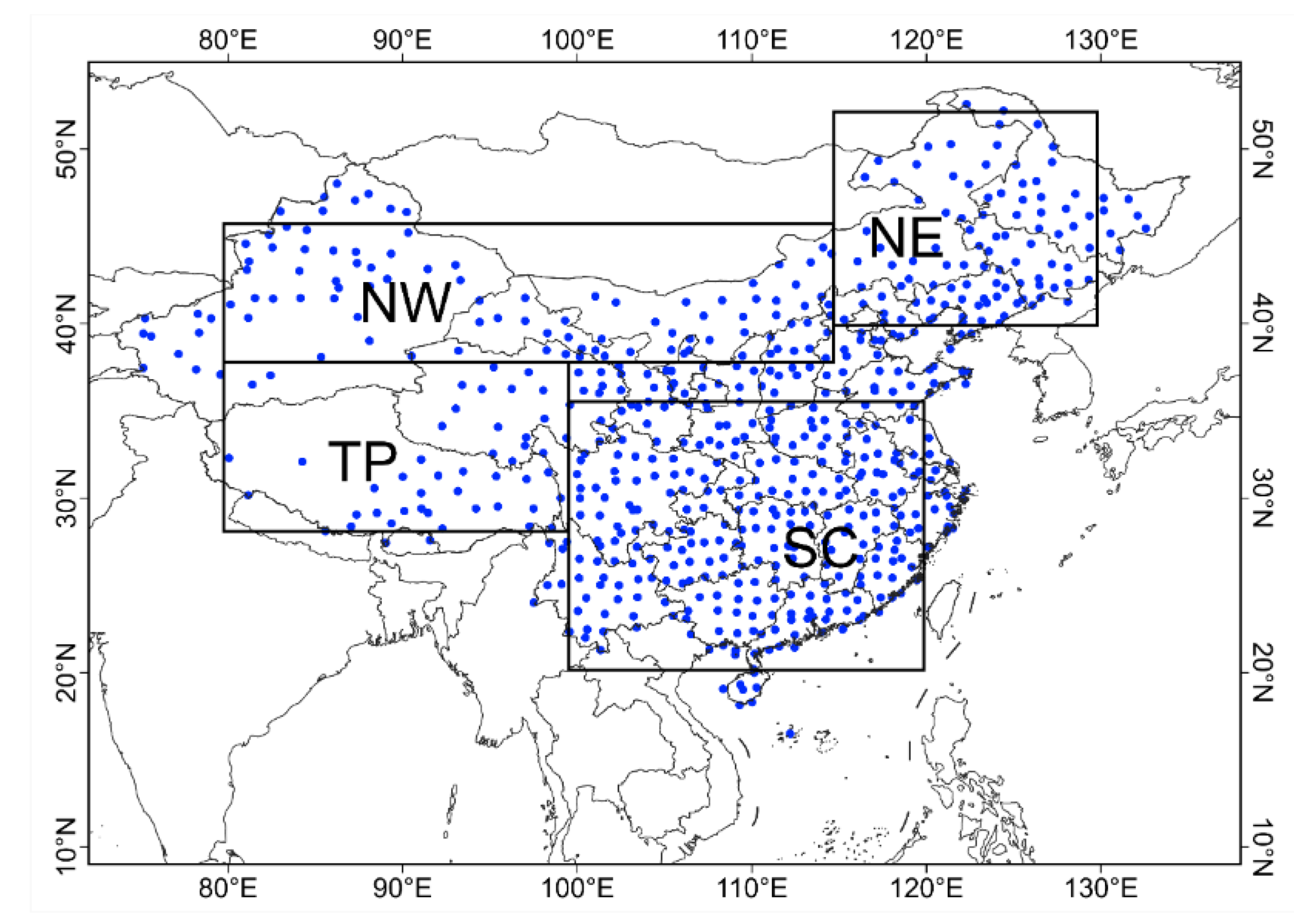
2.2. Station Cloud Amount Data

To evaluate the reliability of satellite products, the homogenized station total cloud amount dataset developed by Xia et al. [47] is used in this study. This dataset was originally based on the surface station observations of monthly total cloud amount (TCA) at 614 meteorological sites of China Meteorological Administration (Figure 1), and is available from the Climate Data Center, China Meteorological Administration (CDC/CMA). The number of sites gradually increased from 340 in 1954 to 680 by 1960, and then remained stable. Note that climate observations are often influenced by changes in station location, exposure of the observational site, instrumentation type, or measurement procedure, and thus they may be subject to shifts in the data records. To generate a homogenized dataset, the RHtestV2 software package was adopted to detect and adjust for multiple shifts that could exist in the original TCA series, as described in Xia et al. [47]. Here, the 614 stations that reported data from 1982 to 2005 were selected to generate the homogenized dataset.
For the comparison of station data with the gridded satellite data (1° × 1°), the station data are interpolated to the 1° × 1° grid using iterative correction objective analysis, which is widely used in meteorological research from the NCAR Command Language (NCL).

2.3. Variables for Comparison and Methodology

In this study, the TCA, high-level cloud amount (CAH), mid-level cloud amount (CAM), and low-level cloud amount (CAL) will be used for analysis. The clouds at different levels are classified by cloud top pressure (CP) with the thresholds used in the ISCCP [31], i.e., CAH (CP < 440 hPa), CAM (440 hPa ≤ CP < 680 hPa), and CAL (680 hPa ≤ CP). For better comparison, note that the GEWEX Cloud Assessment database only keeps the uppermost cloud layer in the case of multilayered clouds. Clouds at the middle level or low level refer to the portion of clouds that are not overlaid by the clouds above, and thus, their CAMs and CALs may be underestimated compared to the real cloud amount when there are multilayered clouds present [18].
When not specifically mentioned in the text, climatological averages are computed over the years when the observations are available (Table 1). For seasonal results, winter refers to December–February (DJF), spring refers to March–May (MAM), summer refers to June–August (JJA), and fall refers to September–November (SON). To compare the satellite data with the site data, the site data are interpolated to a 1° × 1° grid.
To better quantify the differences among the cloud observations in different climatic regimes, China is divided into four subregions in this study, as shown in Figure 1. The northwestern region (NW, 38°N–46° N, 80°E–115° E) is dry throughout the year. The northeastern region (NE, 40°N–52° N, 115°E–130° E) is humid and cloudy in summer, but dry and less cloudy in winter. The Tibetan Plateau region (TP, 28°N–38° N, 80°E–100° E) has a higher altitude, and southern China (SC, 20°N–35° N, 100°E–120° E) is a typical monsoon region with summer convective clouds and large amounts of stratus in winter.

3. Results

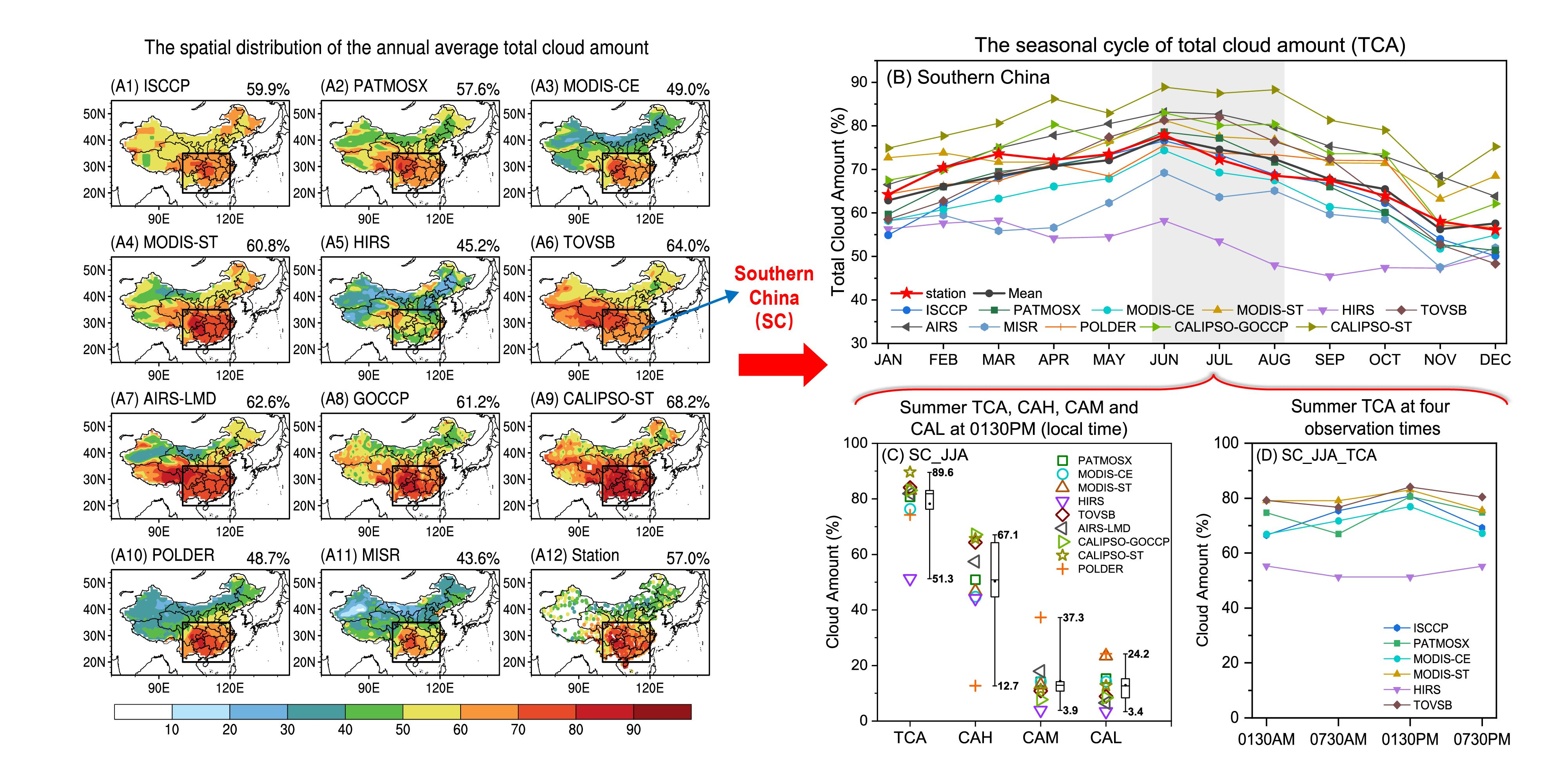
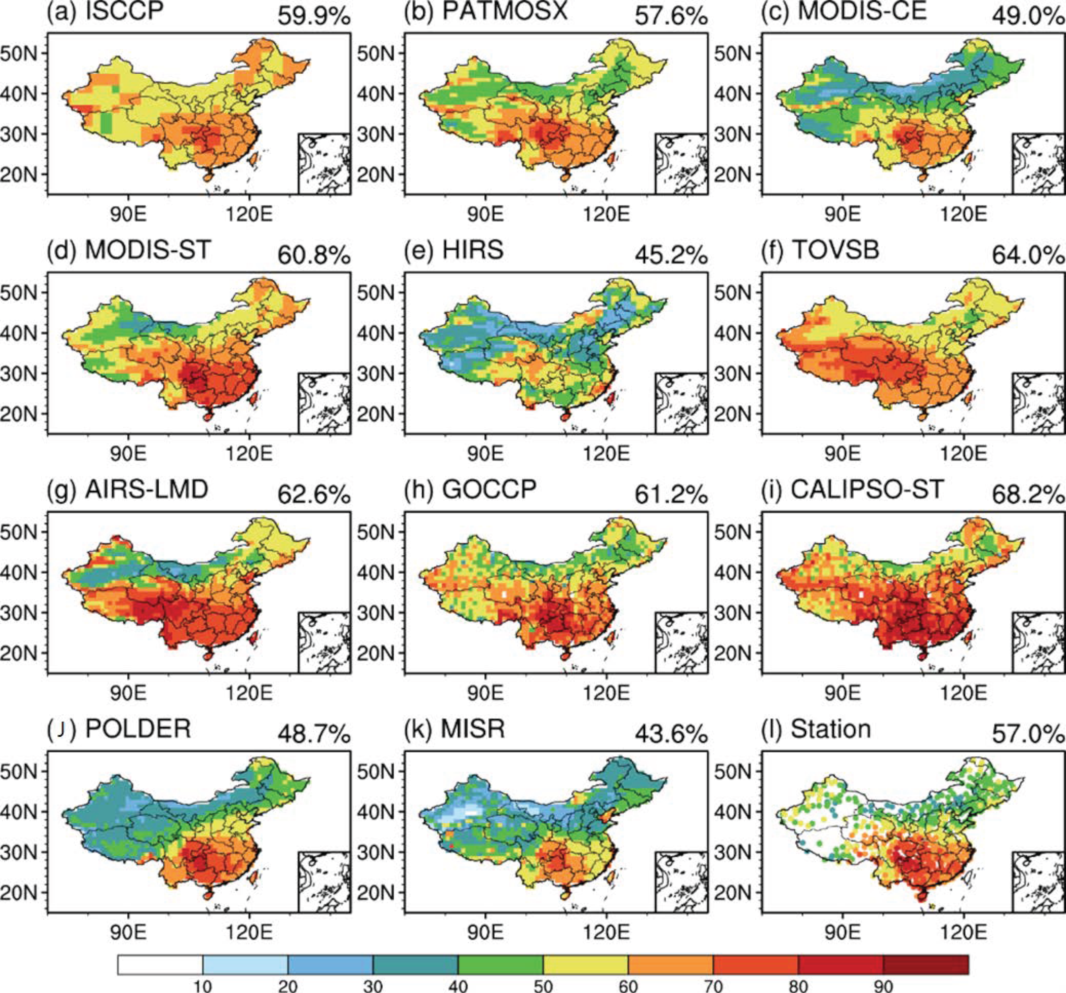
3.1. Spatial Distribution of Clouds in China

Figure 2 shows the spatial distribution of the annual mean TCA over China for 11 satellite-retrieved datasets and meteorological station observations. From the ground observation map (Figure 2l), it is found that the TCA gradually decreases from south China to north China and towards the dry areas in northwest China, with the largest TCA found over the Sichuan Basin and adjacent regions east of the Tibetan Plateau. The annual mean TCA can reach up to 80% in the Sichuan Basin, while it is less than 30% in some areas of Inner Mongolia and even lower than 10% in a large part of Xinjiang. We can see from Figure 2 that most satellite datasets can reproduce similar spatial patterns to the station observations, including the ISCCP, PATMOSX, MODIS-CE, MODIS-ST, GOCCP, POLDER, and MISR. However, the HIRS dataset could not reproduce the maximum TCA center in the Sichuan Basin, with an underestimated TCA value of 50–60% in the region. For the TOVSB dataset, the region with the maximum annual TCA is found from Sichuan to the regions further west, including the Tibetan Plateau and part of Xinjiang, which is inconsistent with the station observations. For the CALIPSO-ST and AIRS-LMD datasets, although a larger TCA could be found in Sichuan and south China, the region with a large TCA is more geographically extended compared with the observed TCA distribution, especially for the CALIPSO-ST product. The cloud amount in Xinjiang is distinctly overestimated in the CALIPSO-ST product.
Overall, the annual averaged TCA over China measured by station observations is 57%, but the annual TCAs across the individual datasets differ by 25% on average, ranging from 43.6% to 68.2%, with the largest regional averaged TCA being 68.2% for CALIPSO-ST (Figure 2i) and the smallest TCA being 43.6% for MISR (Figure 2k). The TCA derived from PATMOSX is 57.6%, which is the closest to the observed coverage. The TCA from the ISCCP is also close to the observed measurements, with an average amount of 59.9%. However, the CALIPSO-ST TCA is much higher than the observed value, with a TCA of 68.2%, while the TCAs from HIRS and MISR are the lowest, with a TCA of 43.6% for MISR and 45.2% for HIRS.
The aforementioned differences in the TCAs can mainly be explained by the different instrument sensitivities and inversion methods used. The active lidar used for CALIPSO-ST and CALIPSO-GOCCP is a highly sensitive measurement that can even detect subvisible cirrus, which is why the TCA in the CALIPSO dataset is larger than the ensemble means of all of the datasets (Figure 2h,i). In addition, CALIPSO-ST detects 8% more cloud than CALIPSO-GOCCP in China, which can be ascribed to the different horizontal averaging methods and cloud detection thresholds used in the two algorithms, as stated in Section 2. IR sounding along the CO2 absorption band (HIRS-NOAA, TOVSB, AIRS-LMD) and methods that implement IR spectral differences (MODIS-ST) are also powerful for thin cirrus identification. Using CERES classification algorithms, MODIS-CE showed a lower sensitivity than MODIS-ST, leading to approximately 10% fewer clouds in China compared with the MODIS-ST dataset (Figure 2c,d). The amount of cloud in MODIS-ST is less than that of CALIPSO-ST by 7% due to its lesser sensitivity when detecting very thin cirrus clouds in MODIS. The use of HIRS-NOAA is less efficient for detecting low-level clouds, especially those over land with a minimal thermal contrast, as stated in Section 2. Therefore, the difference in the cloud amount in HIRS-NOAA relative to the ensemble mean shows an obvious land–sea contrast, with a lower cloud amount over land (Figure 2e). The TCA of POLDER is in the lower range reported for all of the datasets because only clouds with optical depths larger than 2 are accounted for (Figure 2g). The threshold optical depth value is much larger than 0.1, which is the value used for the ISCCP (during the day), CALIPSO-GOCCP, PATMOS-x, MODIS-ST, AIRS-LMD, HIRS-NOAA, and TOVSB. The cloud amount of MISR refers to clouds for which the stereoscopic cloud height may be determined. Since cloud detection over land is more difficult, MISR shows less sensitivity when detecting thin cirrus clouds over the land than over the ocean. Therefore, compared to the other datasets, MISR tends to provide the lowest TCA over land in China (Figure 2k).
Figure 3 shows the ensemble mean and standard deviations of the annual and seasonal cloud amounts (total, high-level, middle-level, and low-level) from 11 cloud datasets in four subregions of China, i.e., northeast, northwest, south China, and the Tibetan Plateau. In this study, we firstly calculate the regionally averaged results for each set of cloud amount data, and then calculate the ensemble mean and standard deviation of the 11 satellite datasets. The annual mean TCA is the largest over SC (68 ± 7.9%) and second largest over the TP (56 ± 11.5%), while it is relatively small in NE (50 ± 8%) and NW (45 ± 9.9%) China. The TCA in summer also shows similar characteristics; the largest TCA in the SC region reaches 75%, and the smallest TCA in the NW region has a magnitude of around 50%. The characteristics of winter are different from those of summer, with the minimum TCA of 41% found in the NE region. Moreover, the TCA in summer is larger than that in winter in all regions. The region with the largest seasonal difference between TCA in winter and summer is the NE region, with an average difference of up to 18%, and the smallest difference of 6% occurs in the NW region. The standard deviations of TCA for annual mean, winter, and summer range from 7.2 to 15.2%, with the largest standard deviation occurring in the TP region in winter and the smallest standard deviation occurring in the SC region in winter. Of the four regions, the TP shows the largest standard deviations, indicating that the largest range among the 11 datasets occurs in this region, while SC shows relatively smaller standard deviations compared to the 11 datasets.
For clouds at different levels, the CAH class makes up a higher proportion than the CAM and CAL classes in general. The largest CAH is in the TP and SC regions and occurs in summer, reaching 47%, while the smallest CAH occurs in the NE region in winter, reaching 8.5%. The contrast of the CAH value between winter and summer is larger than that of TCA in the NE, NW, and SC regions. The standard deviations of the CAH are also larger than those of the TCA in most cases. This suggests a larger dispersion in the CAH values among datasets than that of the TCA. The CAM value is smaller than the CAH in most cases, with magnitudes of 13–26%, and shows less seasonal variability between summer and winter in most regions, excluding SC, where the seasonal difference is approximately 10%. The standard deviation of CAM in the 11 datasets is approximately 7.6–10.4%, which is almost on the same order of magnitude as CAM, indicating that the CAM products of the different datasets exhibit larger differences. The CAL is comparable to the CAM in the NE and SC regions, but is only half of the CAM in the NW region. In the TP region, due to the high elevation, there are few low-level clouds, so the CAL is very small in both summer and winter. Similar to CAM, the CAL is relatively larger in winter than in summer, and more low-level clouds can be found in the SC region than in other regions; the largest CAL can reach 21 ± 9.4%.

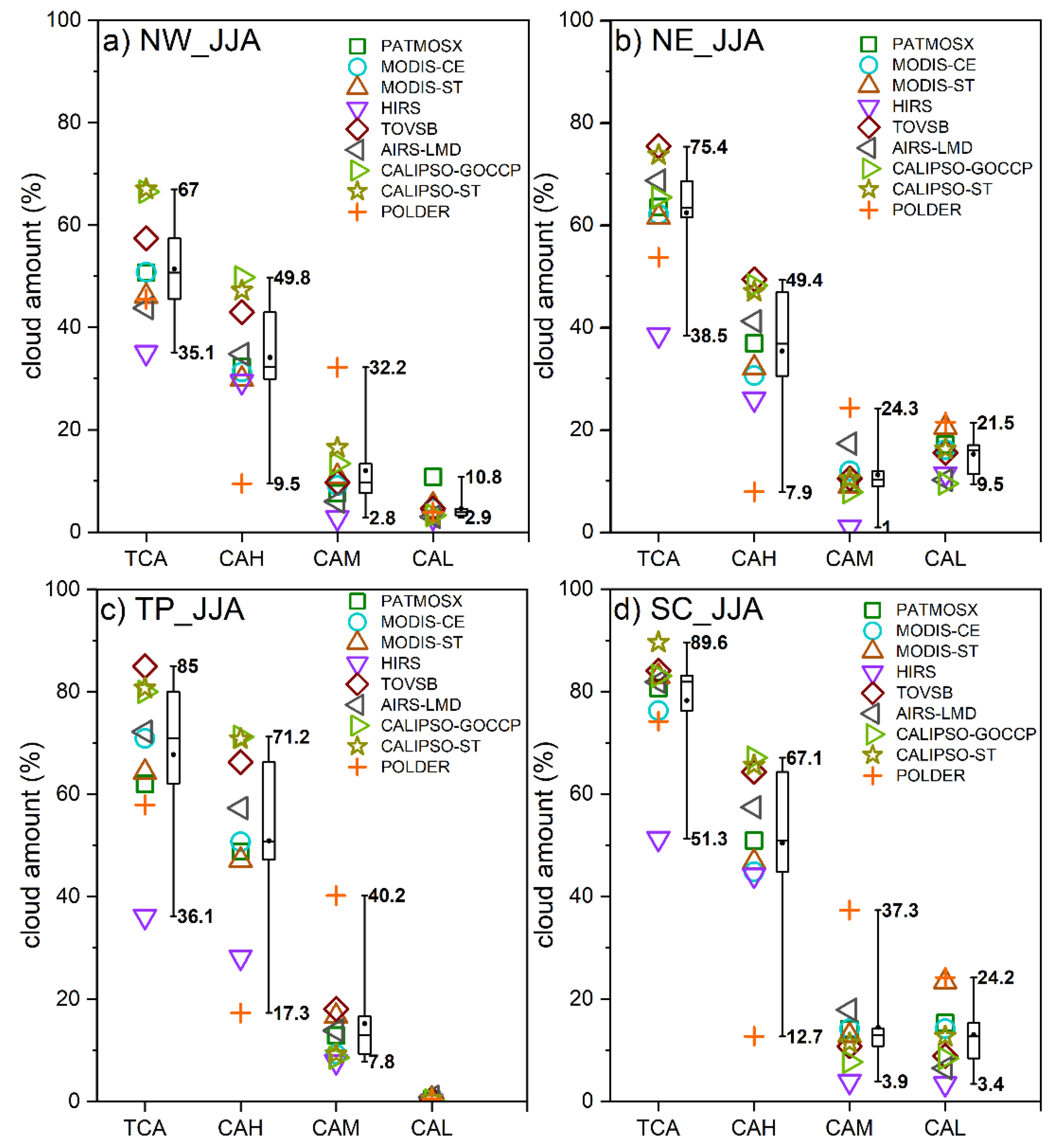
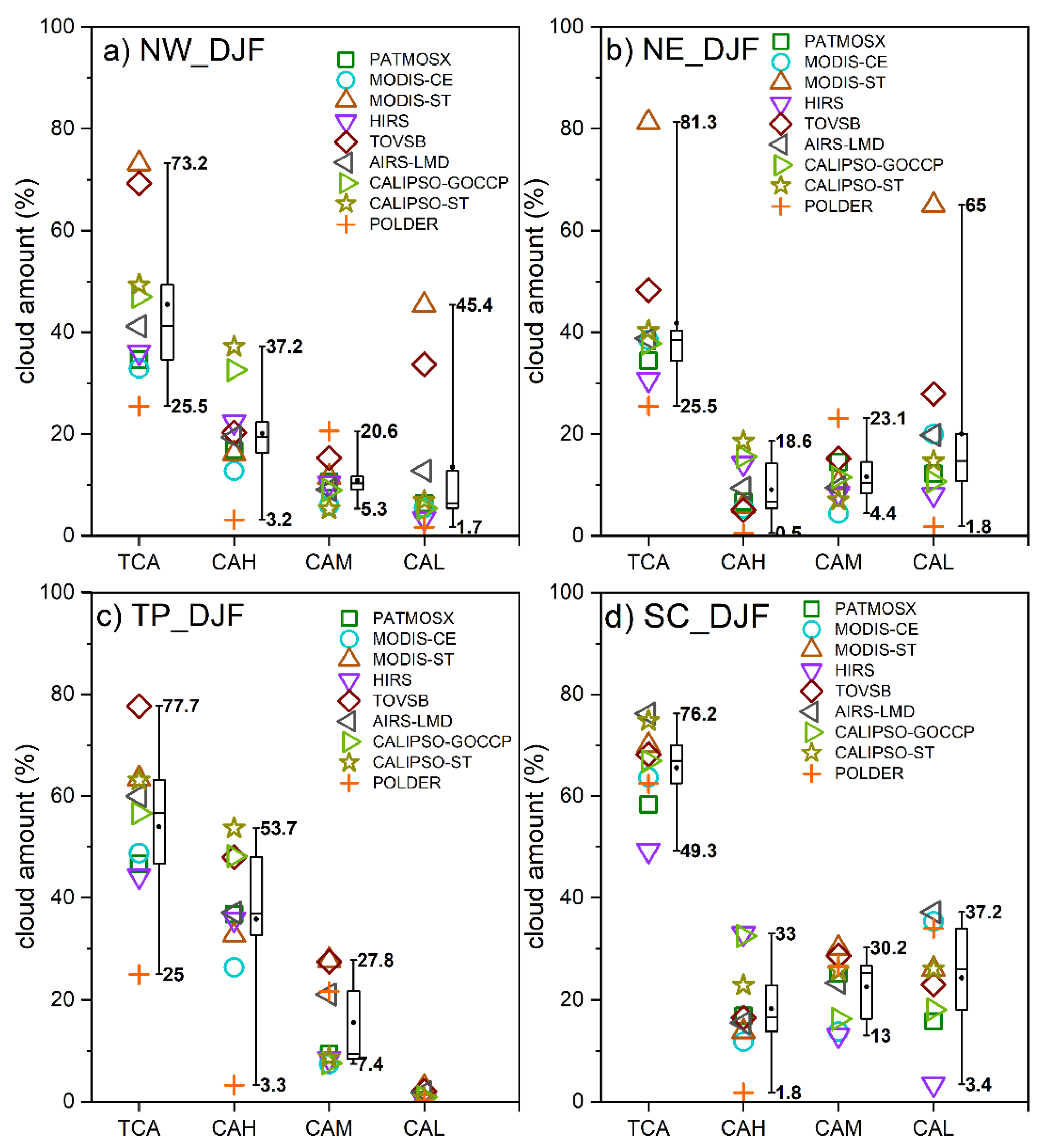
3.2. Influence of Different Instruments and Inversion Algorithms

It is noted that cloud characteristics are very complicated over China, and the satellite datasets exhibit different performances across different regions and seasons. Therefore, the differences and applicability of the different cloud products will be further discussed for the different seasons and regions. In order to quantify the impact of observation instruments or inversion algorithms on the uncertainties of retrieved cloud amount, the satellite cloud amount data with observation time at 13:30 are selected for comparison, and this is because the cloud amount varies at different observation times due to its strong diurnal cycle. Here, neither the ISCCP nor MISR cloud amount datasets are included for comparison, as there is no observation at 13:30 for these datasets.
Figure 4 shows the TCA, CAH, CAM, and CAL in four subregions of China in summer from the nine observation datasets. In the NW region (Figure 4a), the averaged TCA is approximately 50%, and the average CAH is more than 30%, suggesting that CAH accounts for a large proportion (60%) of the total cloud amount. However, the proportions of CAM and CAL are rather low, with approximately 10% of average CAM, and 3% for CAL. In other regions, the CAH is also much larger than the CAM and CAL in summer. Amongst the four subregions, the SC region has the largest TCA, with the average value reaching 78% and an average CAH of approximately 50%. For mid- and low-level clouds, there are fewer single-layer clouds in summer, and the average values of CAM and CAL are less than 20% in all regions.
Among all of the regions, the TP region shows the largest TCA spread from 36.1% to 85%, while the NW region has the smallest TCA spread from 35.1% to 67%. The CAH spread in the SC and TP regions is the largest, while it is relatively small in the NW and NE regions. In addition, the spread of mid-level clouds is significantly larger than that of low-level clouds. When analyzing the range of deviations, it was determined that the results of some of the datasets are very different from those of other datasets, which is the main reason for the dispersion of the observed results. The large CAH spread can be essentially explained by limitations in the instrument’s performance when identifying thin cirrus cloud. As analyzed earlier, the active lidar used for CALIPSO-ST and CALIPSO-GOCCP is highly sensitive. Although the TCA of POLDER is close to the other observational datasets, the CAH is the smallest in all regions. This is mainly because POLDER only considers clouds with optical thicknesses greater than 2 and is insensitive to thin clouds, so POLDER is not suitable for analyzing high-level clouds. The TCA of HIRS is the smallest value obtained across all regions, mainly because HIRS cannot easily identify low-level or middle-level clouds on land, so the HIRS dataset is not applicable to mid- and low-level clouds. In addition to low-level and middle-level clouds, HIRS shows lower high-level cloud amount in TP, which may be ascribed to the lower thermal contrast between the land surface and cloud top in the region compared to the other three regions.
In general, the AIRS-LMD, CALIPSO-GOCCP, CALIPSO-ST, MODIS-CE, MODIS-ST, PATMOSX, and TOVSB datasets are more consistent with the TCA from ground-based observations in summer than the remaining products. Based on these datasets, the spread and standard deviation of the different datasets are recalculated. The dispersion is significantly reduced, and the difference in the TCAs between the four regions is reduced from 33–49% (standard deviation is 10–14%) to 14–23% (standard deviation is 5–10%). The difference in the CAH in the four regions decreases from 40–54% (standard deviation is 13–17%) to 18–24% (standard deviation is 7–11%).
Figure 5 shows the TCA, CAH, CAM, and CAL in the four subregions of China in winter from the nine observation datasets. From the characteristics of the clouds observed in the NW region (Figure 5a), in the TCA (approximately 45%), the high-level cloud class accounts for a relatively large proportion, with an average CAH reaching 20%, an average CAM of approximately 10%, and a CAL of approximately 13%. In the TP region (Figure 5c), high-level clouds also account for a relatively large proportion of the TCA, with an average CAH reaching 30% and an average CAM of approximately 15%. However, in the NE and SC regions, the mid- and low-level cloud classes dominate in winter. In the SC region, the average CAM and CAL are more than 20%, while the CAH is less than 20%. The TCA in the four subregions is in the range of 27–56%, as shown in Figure 5, revealing significant regional variability. The consistency of the results in the SC region is the best, where the TCA spread ranges from 49.3% to 76.2%. The NE region shows the highest TCA values, reaching up to 56%. The range of the CAL in the NE area is the largest, reaching 63%, while the range of CAL in the SC area is the smallest, reaching 34%. It is worth noting that in the NW and NE regions, the larger difference in the TCA is mainly because the TCAs of MODIS-ST and TOVSB are larger than those of the other datasets. In the NW region, there are many high-level clouds. CALIPSO is the most sensitive to thin cirrus clouds. AIRS-LMD and TOVSB also have a strong ability to recognize thin cirrus clouds. However, the TCAs of MODIS-ST and TOVSB are much larger than those of the CALIPSO-ST, CALIPSO-CE, and AIRS-LMD datasets in the NW and NE regions. Wang et al. [19] analyzed the differences in the TCA between the ISCCP products and ground observations and noted that in snow covered areas in the north, satellites sometimes misclassified snow as low-level clouds, resulting in falsely high satellite observations. From the cloud amounts at different heights, the CALs of MODIS-ST and TOVSB are abnormally large, likely due to misclassification caused by snow cover in winter, so the MODIS-ST and TOVSB datasets are not suitable for analyzing clouds in the north in winter; however, this issue does not exist in the south. In conclusion, the AIRS-LMD, CALIPSO-GOCCP, CALIPSO-ST, MODIS-CE, and PATMOSX datasets show the strong ability to identify the TCA and different types of clouds across the different regions.
If the range and standard deviation of the different datasets are recalculated based on these datasets, the results show that the range of TCA is decreased from 27–56% (standard deviation is 8–16%) to 6–18% (standard deviation is 2–8%) in winter. Excluding the TP region, the range of the CALs decreases from 34–63% (standard deviation is 11–19%) to 7–21% (standard deviation is 3–10%). In summer, the range of TCA decreases from 32–49% (standard deviation is 11–15%) to 12–23% (standard deviation is 5–10%). In summary, if the datasets with cloud identification issues are excluded, the range of TCA caused by the observation instruments and inversion algorithms is increased from 6% to 23%, among which the summer observations vary widely, from 12% to 23%, and the difference in winter observations is small, ranging from 6% to 18%.
The results of all observation times were considered in the previous section, while in this section, the influence of the observation time is excluded. The standard deviations of TCA in the NW, NE, TP, and SC regions in the previous section are different from those reported in this section, suggesting that the observation time can have an impact on the dispersion of the satellite cloud amount products.

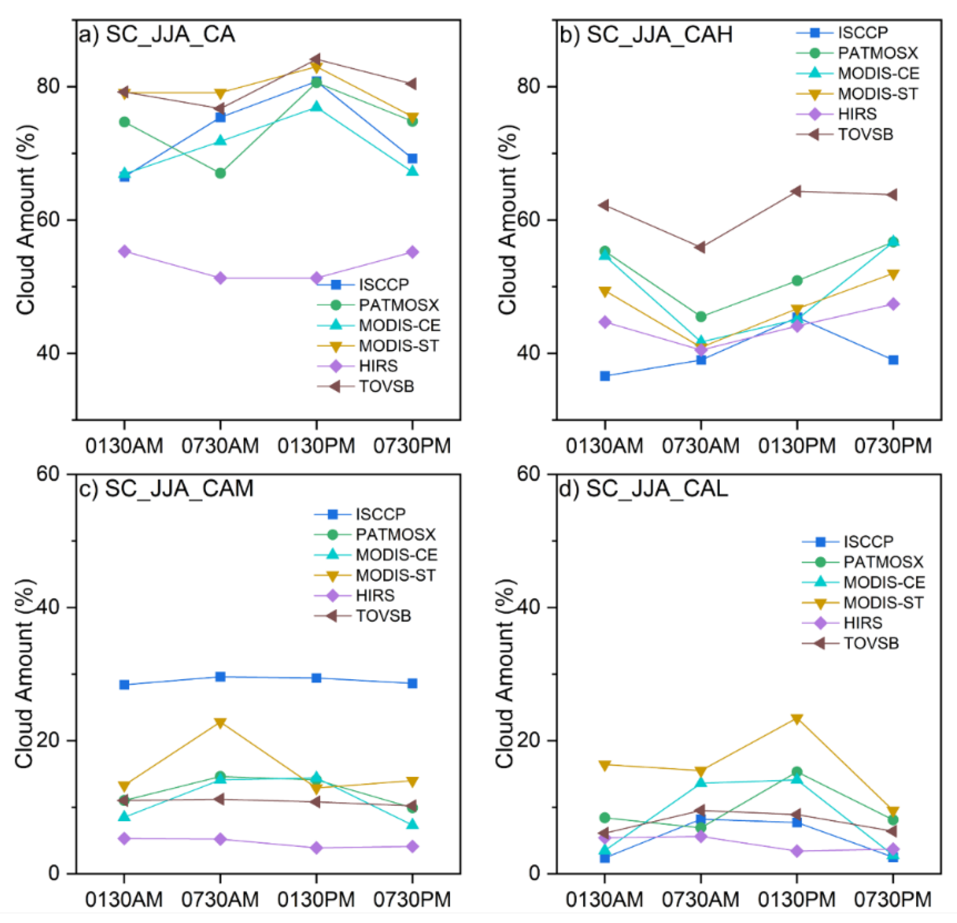
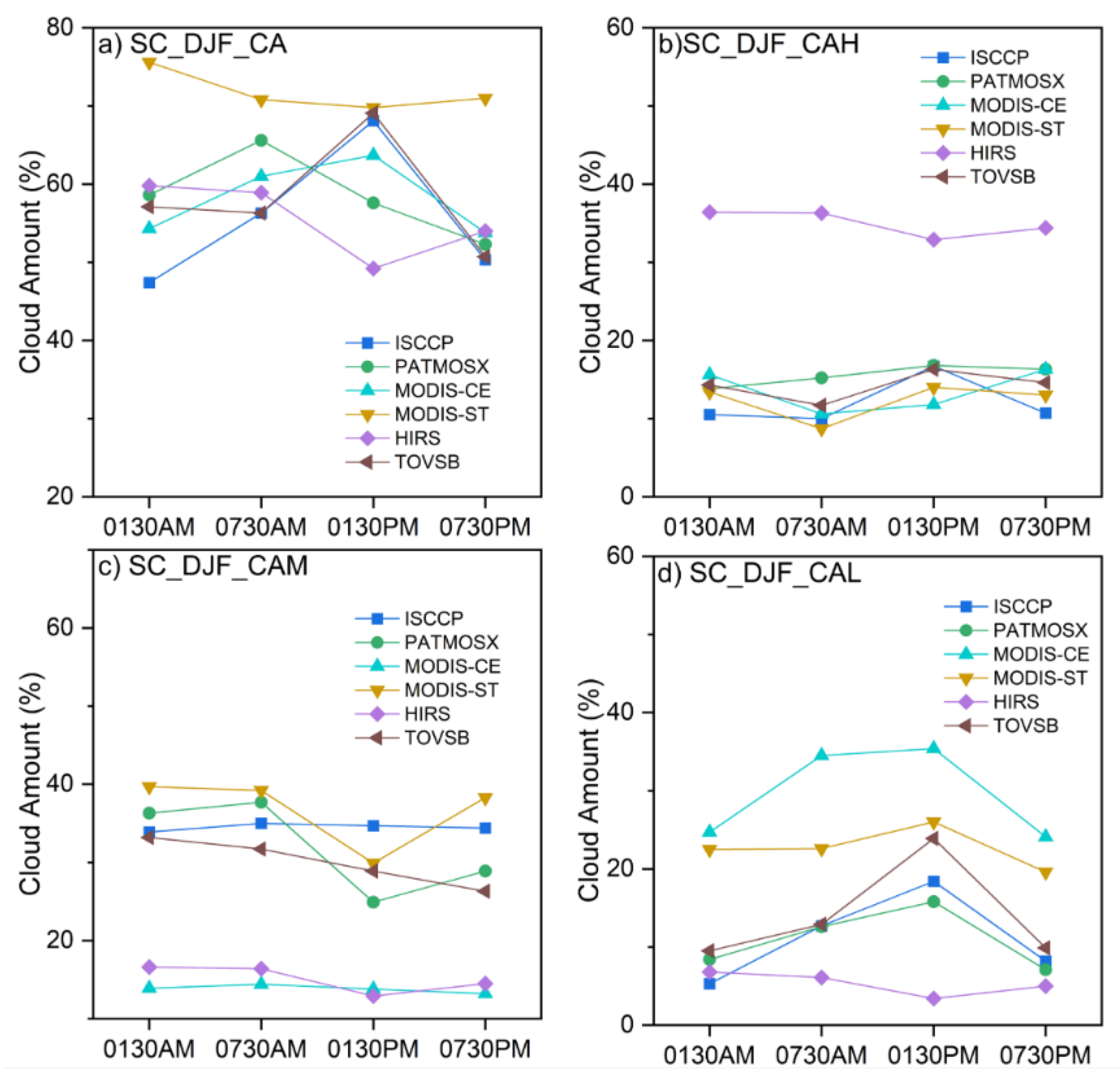
3.3. Impact of Observation Time on Satellite Observations

In order to quantitatively understand the contribution of observation time on the TCA difference amongst 11 satellite datasets, we further present the observation time and the corresponding TCA over SC in Table 2 (summer) and Table 3 (winter) for each satellite cloud dataset, as well as the mean cloud amount averaged over all observation times and different satellite datasets.
In summer (Table 2), based on the observation results collected at different times, the TCA is largest in the afternoon. The observation result of the ISCCP dataset at 0300 PM is 80.8%, and the average observation result of all other satellite datasets at 13:30 reaches 78.4%. The average observation result at 0730 AM is the smallest, reaching 65%. The difference in the TCA between the different datasets in the afternoon is the largest, reaching 38.3%. From the results of the daily variability in the TCA in the different datasets, the summer diurnal change in the TCA of the ISCCP dataset is the largest, reaching 14.3%, followed by PATMOSX, reaching 13.6%. The daily change in the TCA of the remaining datasets does not exceed 10%.
The diurnal variation in the TCA in winter (Table 3) is similar to that in summer, and it also reaches its maximum in the afternoon. Among them, the observation result of the ISCCP dataset at 0300 PM is 68.1%, and the average result of the other datasets is 66.4%. In the afternoon, the range of the different datasets is the largest, reaching 26.9%. From the perspective of the diurnal variation seen in the different datasets, the dataset with the largest diurnal variation in the TCA in winter is ISCCP, reaching 20.7%, followed by TOVSB and AIRS-LMD, both of which exceeded 18%. In general, the diurnal variation in the TCA in south China in winter is greater than that in summer.
Generally, the results for the NW, NE, and TP regions (shown in Supplementary Materials) are similar to those for the SC region. The total cloud cover in these three regions also reaches the maximum in the afternoon, the diurnal variation in winter is greater than in summer, and the ISCCP dataset has the largest diurnal variation in all regions in summer, which is consistent with the results in the SC region. However, in winter, the diurnal variation of the PATMOSX dataset is even larger, reaching 36.9% in the NW region.
To further quantify the impact of the diurnal cycle on the uncertainties of TCA between different datasets, six datasets with four observation times per day were selected for comparison: the ISCCP, PATMOSX, MODIS-CE, MODIS-ST, HIRS, and TOVSB datasets. The observation time of the ISCCP dataset lags by one and a half hours behind the other four sets of data.
Figure 6 and Figure 7 show the TCA and the cloud amount at different heights at four observation times in summer and winter, respectively. For most datasets, the TCA is the largest at noon and the smallest occurs at night, which is consistent with previous research [48], indicating that the formation of land clouds is affected by the underlying surface temperature or the effect of local geothermal convection caused by heating. According to the results of Liu et al. [48], the peak CAL appears at the same time as the peak TCA, while the high-level cloud shows a different feature; the maximum cloud amount appears during the period ranging from afternoon to night. In addition, the unique circulation caused by topography in China regulates the time of the peak high-level cloud amounts. Therefore, the peak CAH appears at 18:00, but in the lower reaches of the Tibetan Plateau, the peak CAH lags to 03:00. The similar diurnal cycle feature of the high- and low-level clouds can be found in Figure 6 and Figure 7. It is also found that the different datasets have different diurnal cycles of the TCA, resulting in different dispersions between the datasets at each observation time. For example, the TCA of PATMOSX in summer varies from 67% to 80.6%, with the TCA being the largest in the afternoon and smallest in the morning and evening. Conversely, the TCA of HIRS is the smallest in the afternoon and largest at night. This results in a greater dataset dispersion in the afternoon. At different observation times in summer, the differences between the datasets range from 23.9% to 32.8%, with the largest difference occurring in the afternoon and the smallest difference occurring in the early morning.
According to the analysis described above, HIRS has erroneous observations of the TCA. HIRS shows a diurnal cycle with the smallest TCA in the afternoon and the largest cloud amount at night, which is the opposite of the other datasets. This is mainly because HIRS poorly identifies low- and mid-level clouds. Therefore, the diurnal cycle of TCA in the HIRS dataset is similar to that of CAH. If the HIRS dataset is excluded, the range of TCA observations is reduced from 23.9–32.8% to 7.2–13.2%. There are also issues with the diurnal cycling of cloud amounts of different heights introduced by using the ISCCP dataset. These problems may result from the misclassification of thin and high-level clouds above the low-level clouds as mid-level clouds, and may also be due to the worse inversion results reported at night than during the daytime. Further investigation into the calibration and algorithm is needed to uncover the reasons for the erroneous diurnal cycles of TCA by HIRS.
The diurnal cycle of the TCA in winter is similar to that in summer. The difference between the datasets ranges from 14.5% to 28.2%. The difference between the observations is the smallest in the morning and is the largest at dawn. In addition to the aforementioned issues associated with the HIRS dataset, the diurnal cycle of MODIS-ST is also the opposite of that of other datasets, mainly because the CAL is significantly larger at night in winter. If the MODIS-ST and HIRS datasets are excluded, the range of TCAs can be reduced from 20.6–28.2% to 4.5–11.5%. The TCA deviation range of the different observation times is far less than the difference of approximately 20% resulting from the different observation instruments or inversion algorithms.

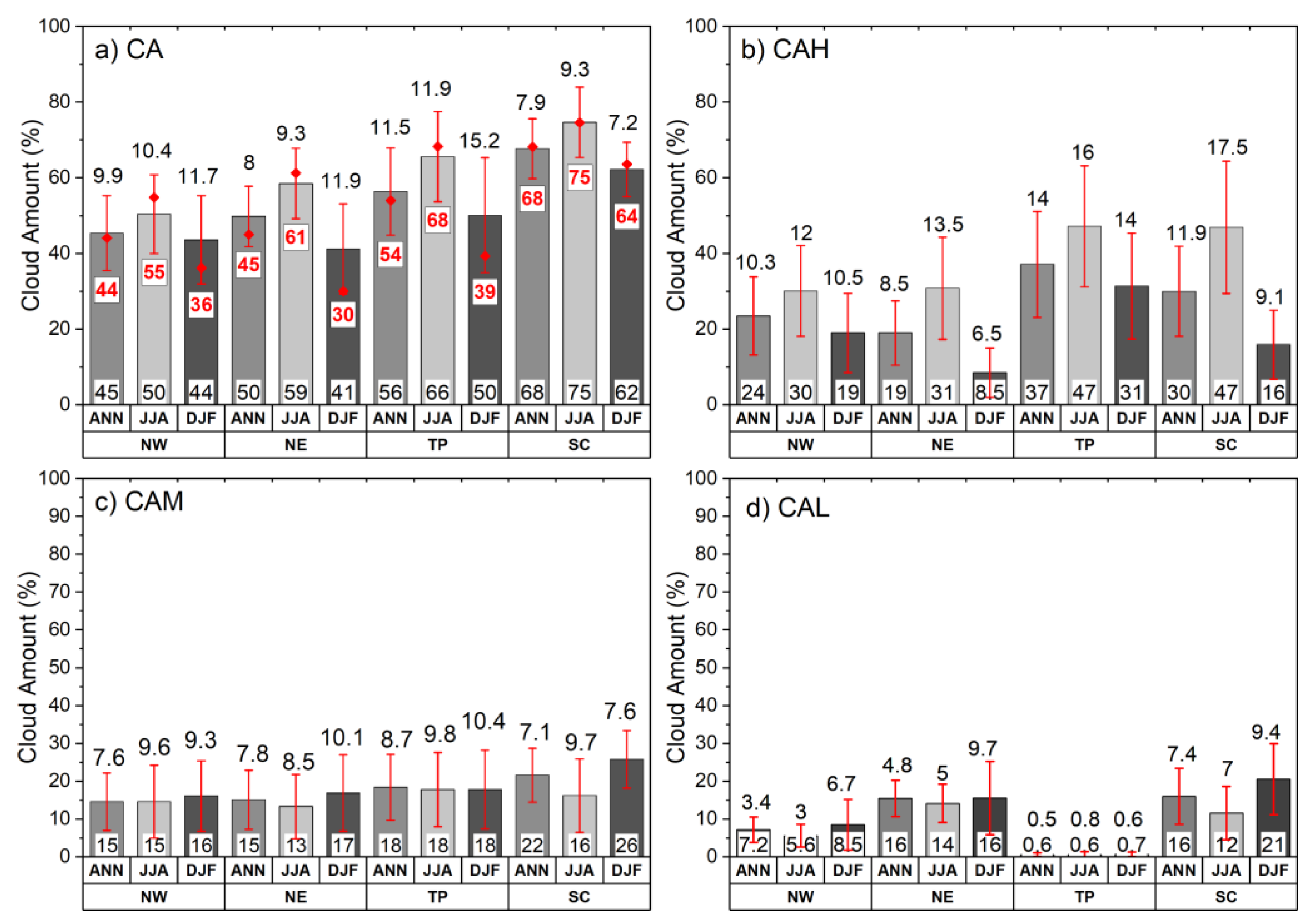
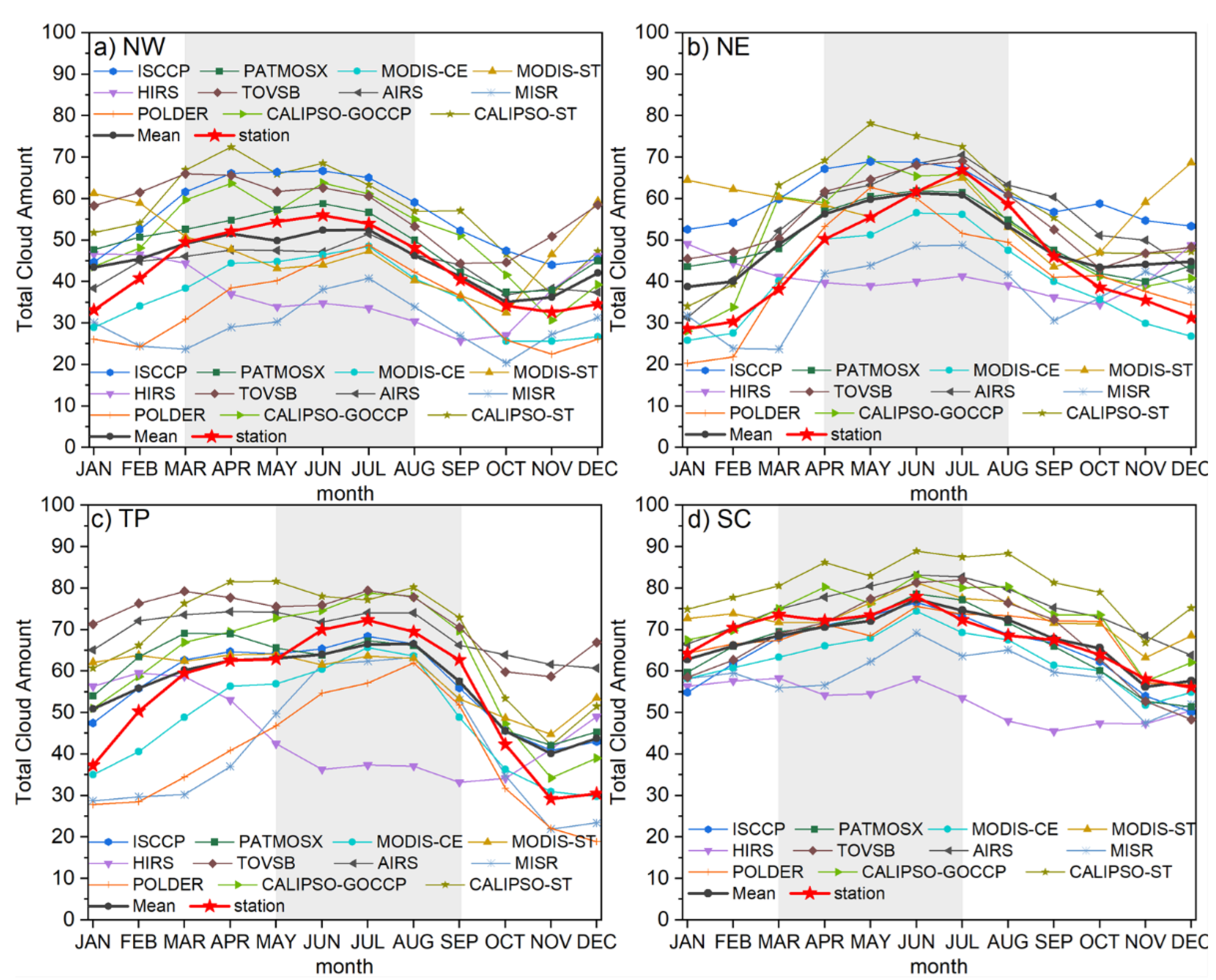
3.4. Seasonal Variations of Cloud Amount

Figure 8 shows the seasonal variations in the TCA for each dataset and the ensemble mean across the four regions. The yearly peaks are also shown in the gray area. The station data show that there are distinct seasonal variations in the cloud amount across the four regions. In the NW region, the maximum value of TCA is 56%, which appears in June, and the minimum value is 32.6%, which appears in November, with a span of 23.4%. In the NE region, the maximum value of TCA appears in July, reaching 66.9%, and the minimum value appears in January, reaching 28.7%. The TP region has the largest seasonal variation, with the difference between the maximum value in July (69.9%) and the minimum value in November (29.2%) reaching 43.1%. The SC region has the smallest seasonal variation of only 21.9%, of which the maximum value occurs in June (78%) and the minimum value occurs in December (56.1%). Most datasets show similar seasonal variability, with the largest cloud amount occurring in summer and the smallest cloud amount occurring in fall and winter in most datasets, although the magnitudes are quite different. Slight regional differences in the seasonal cycle can also be found, with the peak ensemble mean TCAs found in June for the SC, NE, and NW regions, but in July and August for the TP region. Of the four regions, SC shows the smallest standard deviation among all datasets for all 12 months, with the smallest standard deviation seen in February and the largest standard deviation seen in August. The TP region shows the largest standard deviations for all 12 months, with a minimum standard deviation in October and a maximum standard deviation in February and March. Despite the similarity between most datasets, there are some datasets that show quite different seasonal variation features from the other compared datasets in certain regions. In the NW and NE regions, the TCAs from MODIS-ST and HIRS show their peaks in December and January, and the smallest TCAs are found in September and October. In the TP region, the HIRS TCA shows the smallest cloud amount from June to October and the largest cloud amount from January to March, which is the opposite of the features seen in other datasets.
Note that the satellite estimates of TCA (in terms of the means of multiple datasets) are systematically larger than the ground-based observations in winter in most regions (except SC). This can be explained by the fact that the northern China and Tibetan Plateau regions are covered with snow at times in winter, and snow may be misjudged as low clouds in satellite observations, leading to the overestimation of TCA [49]. In addition, the northern region is mainly covered by thin high clouds in winter, which may be missed by the station observation made manually by the meteorological observers. This underestimation of station observation may be more pronounced at night.

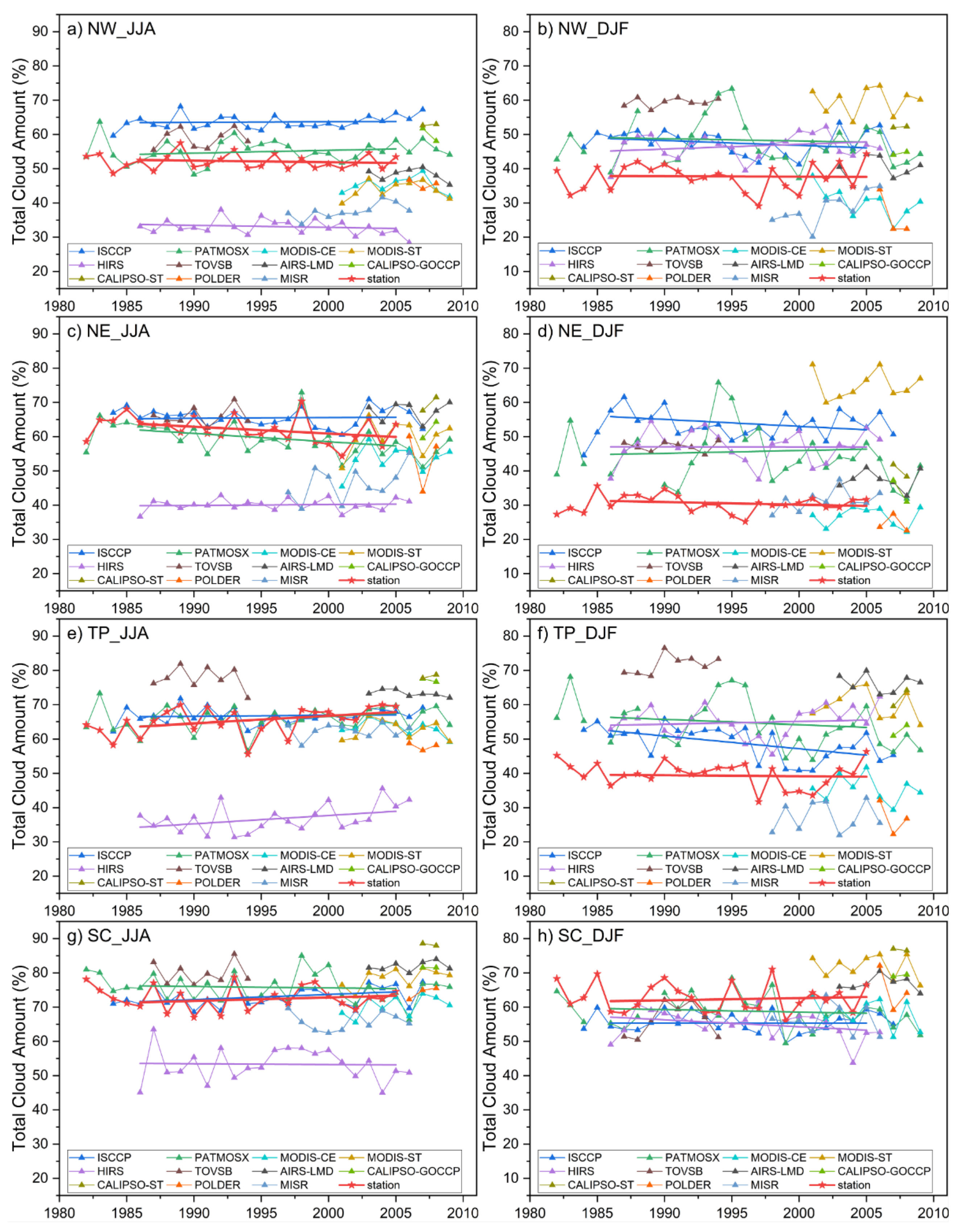
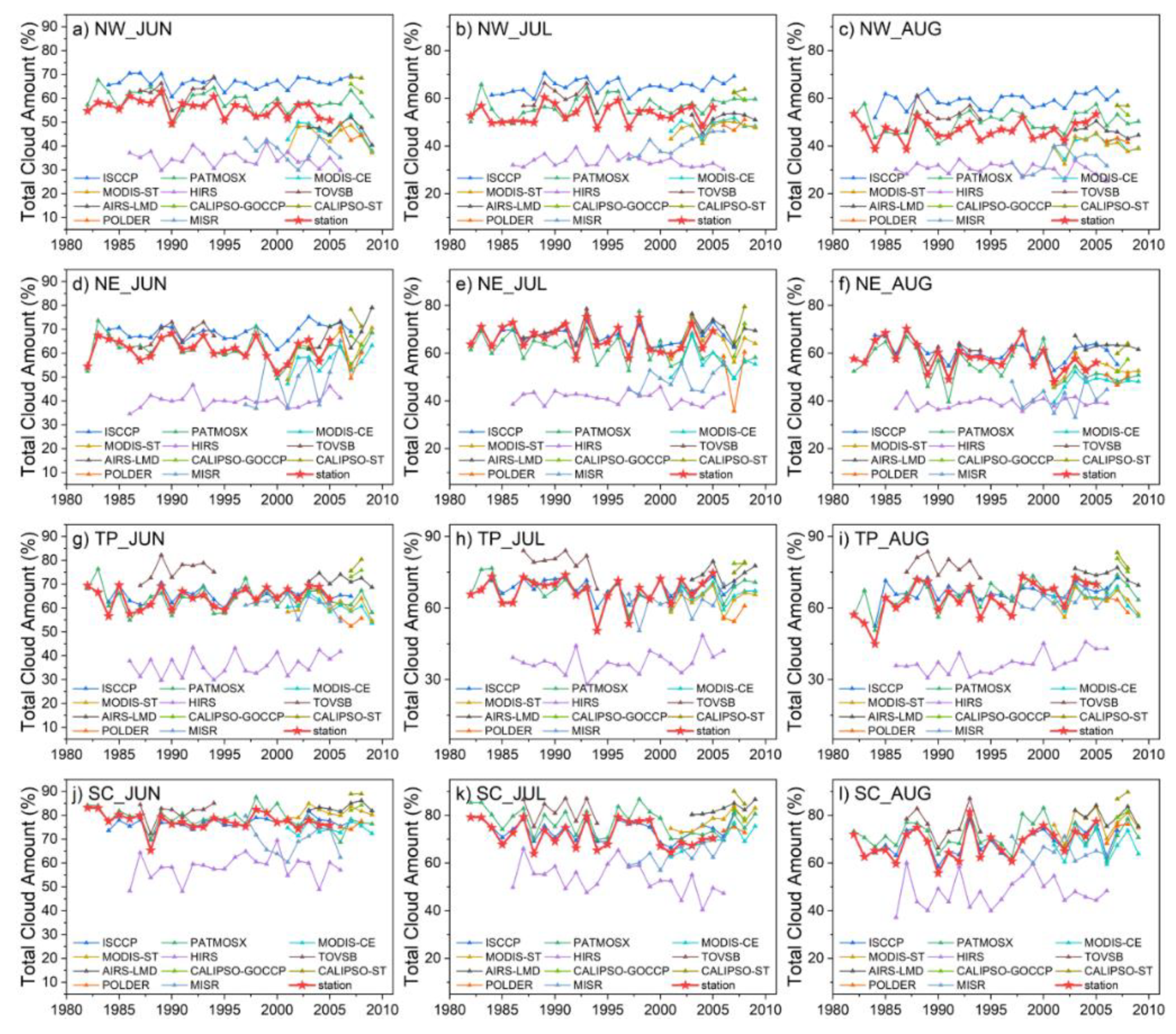
3.5. Interannual Variations and Trends

Figure 9 shows the interannual variations in the TCA in summer and winter across the four regions. From the results of the TCA derived from the site data, it can be seen that there are differences in the interannual variability of the TCA across the different regions. In summer, the NW region has the smallest interannual variability of only 2.1%. The summer interannual variabilities in the NE, TP, and SC regions are 3.8%, 3.8%, and 3.3%, respectively. The SC area in winter is the area that shows the most significant interannual variability of 4.4%. The other three regions report values of 3.8%, 2.6%, and 3.8%. In summer, except that the TCA of the HIRS dataset is relatively small in all regions, other datasets are close to the site data, especially in the TP and SC regions, where the satellite observation results are more concentrated. The interannual variation of TCA in winter is greater than that in summer, especially in the NW, NE, and TP regions. The results of satellite data in winter are highly dispersed, and only the data in the SC region are concentrated.
The temporal correlation coefficients of the TCA between the satellite datasets and site data in the NW, NE, SC, and TP regions are calculated and shown in Table 4. For correlation calculations, the observation periods need to be long enough. Only the products with more than 5 years of the same observation year are selected to calculate the correlation coefficients. In total, seven datasets (HIRS, ISCCP-D1, MISR, MODIS-CE, MODIS-ST, PATMOSX, and TOVSB) are used to calculate the correlation coefficients (Table 4).
In summer, the temporal correlation coefficients of TCAs between most satellite datasets and site data are greater than 0.7, which indicates that the results of the satellite datasets are consistent with the site data, except for HIRS. In winter, the SC region and the TP region are the regions with the best correlation between the TCA of satellite observations and the TCA of the site data, while the NE region is the region with the worst temporal correlation. In general, ISCCP-D1, MODIS-CE, and MODIS-ST have the best correlation with the site data, and the temporal correlation coefficient can reach more than 0.5 in all regions. The TCA of the PATMOSX dataset also has high temporal correlation with that of the site data, except for the NW and NE regions in winter.
Note that two satellite products (MISR and TOVSB) deviate significantly from the station observations, with a low correlation coefficient (around zero) in certain seasons (summer for MISR, winter for TOVSB). This may be linked to the caveats in the algorithm or calibration of these satellite retrievals, and further investigation is needed to uncover the reasons.
For trend analysis, three datasets with more than 20-year observations (HIRS, ISCCP, PATMOSTX) are used for the comparison with station observation (Figure 9). The station observations show that TCA decreases with a linear trend of −0.05/year and −0.01/year for summer and winter, respectively, in NW during 1986–2005. The TCA also decreases in NE, but with a stronger decreasing trend (−0.2/year and −0.08/year for summer and winter, respectively) than in NW. Different trends of TCA are found for summer (0.22/year) and winter (−0.03/year) in TP. In SC, there is an increasing trend of TCA in both summer (0.1/year) and winter (0.06/year).
Compared to the station observation, none of the three datasets (HIRS, ISCCP, PATMOSTX) capture the trend of TCA except in TP, where all three datasets show an increasing trend of summer TCA. In particular, the increasing trend of summer TCA in TP shown in HIRS (0.24/year) and PATMOSTX (0.19/year) is close to the station observation (0.22/year). PATMOSTX also captures the decreasing trend of summer TCA in NE well (−0.24/year) compared to the station observation (0.2/year). In addition, although HIRS shows the opposite trend of winter TCA in NW (0.14/year) compared to the station observation (−0.01/year), HIRS captures the decreasing trend of summer TCA well, with a similar magnitude (−0.06/year) to the station observation (−0.05/year). Similarly, ISCCP captures the increasing trend of summer TCA in SC (0.15/year), but shows a very weak trend (near zero) compared to the increasing trend of winter TCA in SC (0.06/year). All three datasets show a decreasing trend of winter TCA in SC, which is the opposite of the increasing trend in the station observation. Overall, the three products show different trends of TCA in most regions, and none of them overperforms the other datasets in any region.
Here, the comparison of temporal variations of TCA between satellites and station observations are based on the season mean in summer and winter. In fact, the difference between satellite and station observations for a specific month (e.g., June, July, August) is generally similar to that for the seasonal mean (Figure 10). The root mean square error (RMSE) in monthly TCA between the satellites and station observation is close to that in seasonal mean TCA. This suggests that the conclusion for the difference in seasonal mean TCA can be applied to that for monthly TCA.

4. Discussion

Satellite measurement is the only approach that can provide a continuous survey of cloud distribution at the continental to the global scale and has been widely used for climate change and variability studies, as well as for model evaluation and improvement. The differences in the cloud amount and its seasonal and interannual variation in China found among 11 current cloud products not only reveal the complexity of the cloud features in the East Asian monsoon region, but also demonstrate the large uncertainties and difficulties associated with cloud retrievals from different satellite observations.
This study compares the 11 satellite cloud products with ground station observations. However, it should be noted that the ground station data themselves also involve a considerable amount of uncertainty, especially in the Tibetan Plateau, where the ground stations are sparsely distributed. Meanwhile, the interpolation of station data to grid points also introduces new errors. In the future, cloud products in the Tibetan Plateau should be further evaluated so that they can be better applied in model evaluation and climate research.
The remarkable differences in the cloud amounts over China can be attributed to the different sensitivities of the observational instruments to thin clouds (e.g., cirrus) and classification algorithms for each cloud type. The partitioning of the individual contributions from these two factors to the uncertainty associated with cloud detection needs to be further investigated in the future.
In the report of the GEWEX cloud assessment project, only the results of the different situations of the world, land, and sea areas were analyzed, and the conditions in East Asia were not analyzed. However, the principle behind cloud satellite detections and inversion mechanisms are applicable to all regions of the world. For example, the conclusion that the CALIPSO satellites are more sensitive to thin cloud detection, that MISR is not sensitive to cirrus clouds on land, and that HIRS is not sensitive to low-level clouds on land are still applicable to East Asia. However, the simulation results of some models across the individual regions are abnormal, which cannot be explained by the abovementioned reasons. For example, MODIS-ST reports abnormal winter CAL in the NW and NE regions, but no abnormalities in the TP and SC regions. This may be due to the presence of snow in winter, which causes MODIS-ST to misclassify low-level clouds. In this regard, further analysis is needed in the future.
When analyzing the temporal variability of clouds, this report pointed out that day-night and daytime sampling differences among the datasets with no change in method (IR sounders and lidar) reflect random differences expressed in a change in the resulting coverage percentage. CALIPSO seems to have a slightly smaller detection sensitivity for thin cirrus during the day. Day–night differences in the TCA for ISCCP correspond to less than 10% over land. It also pointed out that most datasets show a similar seasonal cycle. These conclusions are more consistent with the analysis results in China.
Cloud statistics depend on the instrument’s retrieval capability to detect clouds. These satellite cloud products are very valuable for climate studies and model evaluation. When they are used for comparisons with climate models, observation times and retrieval filtering must be considered. This can be achieved by the Cloud Feedback Model Intercomparison Project (CFMIP) Observation Simulator Package (COSP) [50]. COSP is a software tool that facilitates the use of satellite data to evaluate models in a consistent way.

5. Conclusions

In this study, we compare the spatial and temporal variations in TCA over China from the 11 datasets provided by the GEWEX cloud assessment project, and use the site data as a reference. Our results show that all of the products show similar spatial distributions of clouds over China, with the largest cloud amount observed in the Sichuan Basin and adjacent regions located east of the Tibetan Plateau, and the smallest cloud amount observed in the arid regions of northern China and Mongolia. However, the magnitude of the annual mean cloud amount differs significantly, with amplitudes up to 40–60% in certain regions, and the regional averaged difference over China reaches 20%. Over the four typical subregions, the largest cloud amount difference among the datasets is found in the TP region, with the standard deviation of the annual cloud amount being approximately 13%; the smallest difference is found in the SC region, with the standard deviation being approximately 9%. Moreover, differences in the cloud amount are larger in winter (17.6% for TP and 11% for SC) than in summer (13.5% for TP and 10.1% for SC). In terms of the different levels of cloud amount, the high-level cloud amount (CAH) is found to exhibit large standard deviations, which are very similar to those for the TCA. In summer, the CAH shows larger standard deviations than the TCA.
The influence of different instruments or inversion algorithms and observation times are further analyzed in this study. First, we discuss the differences and applicability of the different cloud products separately for different seasons and regions after eliminating the influence of observation time. The results indicate that the ISCCP, MODIS-ST, and TOVSB datasets are not suitable for analyzing clouds in the north in winter, but this issue does not exist in the south. The AIRS-LMD, CALIPSO-GOCCP, CALIPSO-ST, MODIS-CE, and PATMOSX datasets show a strong ability to identify the TCA and different types of clouds in different regions both in summer and winter. The difference in the TCA caused by the observation instruments and the inversion algorithms reaches approximately 20%, among which the summer observations vary widely from 14% to 23%, and the difference in winter observations is small, ranging from 6% to 17%. Second, we analyze the influence of the observation time using the ISCCP, PATMOSX, MODIS-CE, MODIS-ST, HIRS, and TOVSB datasets. In summer, the TCA of HIRS shows a diurnal cycle feature, which is the opposite of the other datasets. If the HIRS dataset is excluded, the difference between the remaining observations is reduced from 23.9–32.8% to 7.2–13.2%. In winter, the TCAs of HIRS and MODIS-ST show a diurnal cycle feature in contrast to the other datasets. If the MODIS-ST and HIRS datasets are excluded, the difference between the TCAs can be reduced from 20.6–28.2% to 4.5–11.5%. The TCA deviation range across the different observation times is far less than the difference of approximately 20% caused by the different observation instruments or inversion algorithms.
For the seasonal variations, most cloud products show similar features, with the largest cloud amount in summer and smallest in fall and winter. The standard deviations of the monthly cloud amount are the largest on the TP, ranging from 10.6% in October to 16% in February and March, and they are the smallest in SC, with standard deviations generally less than 8.8%. Furthermore, different seasonal cycles are found in two datasets (MODIS-ST and HIRS) over the northern part of China (NW and NE), where the largest cloud amount is found in winter and the smallest is found in September and October. In addition, in the TP region, HIRS tends to provide a seasonal cycle that is the opposite of the other datasets.
In terms of interannual variation, seven datasets (HIRS, ISCCP-D1, MISR, MODIS-CE, MODIS-ST, PATMOSX, and TOVSB) are selected here to investigate the interannual variability in the TCA. By analyzing the correlation between the interannual variation of the total cloud amount of satellite datasets and site data, it is found that the temporal correlation coefficients of TCAs between most satellite datasets and site data are greater than 0.7 in summer. In winter, the TCAs of satellite datasets in the SC and TP regions are more consistent with the TCA of the site data. The ISCCP-D1, MODIS-CE, and MODIS-ST have better performance in interannual variation. The temporal characteristics of the total cloud amount of PATMOSX in summer are more consistent with the site data than in winter. In general, the temporal and spatial characteristics of the MODIS-CE in China show the best performance when compared with other satellite datasets. As for ISCCP-D1, the temporal variation characteristics are quite consistent with the site data, but there are problems with the spatial distribution.
Overall, the findings from this study further suggest the complicated features of the cloud characteristics over China, and the large uncertainties amongst current satellite cloud products. More caution should be taken when selecting a satellite cloud product for the evaluation of climate model performance in the cloud simulation. In this respect, the results shown here are very useful for the selection of satellite cloud products in different aspects of climate studies, including spatial distribution, seasonal cycles, and interannual variations. For example, some satellite products deviate greatly from the station observation for the interannual variations of TCA for one season, yet can exhibit high reliability for another season (Table 4), and it is therefore necessary to select the product with high reliability for interannual variability studies.
Note that some differences between the satellite measurements and station observations shown in this study may partly result from the uncertainties in the station observations, although these uncertainties are unavailable and, thus, are not provided in the dataset. Therefore, the quantification of measurement uncertainties as well as the further development of station observations are also desirable to improve the datasets for validating satellite measurements. In addition, further improvements to cloud detection methodologies are also necessary for the development of new cloud products for climate studies in the future [51,52].

Supplementary Materials

The following supporting information can be downloaded at https://www.mdpi.com/article/10.3390/rs14092173/s1, Table S1: Total cloud amount across the different observation times and different datasets in summer over NW region (unit: %), Table S2: Total cloud amount across the different observation times and different datasets in winter over NW region (unit: %), Table S3: Total cloud amount across the different observation times and different datasets in summer over NE region (unit: %), Table S4: Total cloud amount across the different observation times and different datasets in winter over NE region (unit: %), Table S5: Total cloud amount across the different observation times and different datasets in summer over TP region (unit: %), Table S6: Total cloud amount across the different observation times and different datasets in winter over TP region (unit: %).

Author Contributions

Conceptualization, Y.W. and Z.L.; data processing, Y.W.; writing—original draft preparation, Y.W.; writing—review and editing, Z.L. and C.W. All authors have read and agreed to the published version of the manuscript.

Funding

This research is supported by the National Key Research and Development Program of China (2017YFA0603503), the National Natural Science Foundation of China (41975119 and 41830966), and the project “Climate monitoring and prediction applications in the high and cold regions of North Hemisphere using FY-3 satellite products” (Grant No. ZQC-R18012) from National Satellite Meteorological Center, China.

Acknowledgments

We would like to thank the Climserv Data Center of IPSL/CNRS for providing the GEWEX cloud assessment datasets, and Xia X. for providing the homogenized station total cloud amount dataset over China.

Conflicts of Interest

The authors declare no conflict of interest.

References

  1. Stephens, G.L. Cloud feedbacks in the climate system: A critical review. J. Clim. 2005, 18, 237–273. [Google Scholar] [CrossRef] [Green Version]
  2. Wild, M.; Folini, D.; Schar, C.; Loeb, N.; Dutton, E.G.; Konig-Langlo, G. The global energy balance from a surface perspective. Clim. Dyn. 2013, 40, 3107–3134. [Google Scholar] [CrossRef] [Green Version]
  3. Quante, M. The role of clouds in the climate system. J. Phys. IV France 2004, 121, 61–86. [Google Scholar] [CrossRef] [Green Version]
  4. Liu, Y.; Wu, W.; Jensen, M.P.; Toto, T. Relationship between cloud radiative forcing, cloud fraction and cloud albedo, and new surface-based approach for determining cloud albedo. Atmos. Chem. Phys. 2011, 11, 7155–7170. [Google Scholar] [CrossRef] [Green Version]
  5. Manabe, S.; Strickler, R.F. Thermal Equilibrium of the Atmosphere with a Convective Adjustment. J. Atmos. Sci. 1964, 21, 361–385. [Google Scholar] [CrossRef]
  6. Norris, J.R.; Allen, R.J.; Evan, A.T.; Zelinka, M.D.; O’Dell, C.W.; Klein, S.A. Evidence for climate change in the satellite cloud record. Nature 2016, 536, 72–75. [Google Scholar] [CrossRef] [Green Version]
  7. Ding, S.G.; Shi, G.Y.; Zhao, C.S. Analyze the changes of global cloud amount in recent 20 years and their implications for climate using ISCCP D2 data. Chin. Sci. Bull. 2004, 49, 1105–1111. (In Chinese) [Google Scholar] [CrossRef]
  8. Ban-Weiss, G.A.; Jin, L.; Bauer, S.E.; Bennartz, R.; Liu, X.H.; Zhang, K.; Ming, Y.; Guo, H.; Jiang, J.H. Evaluating clouds, aerosols, and their interactions in three global climate models using satellite simulators and observations. J. Geophys. Res. Atmos. 2014, 119, 10876–10901. [Google Scholar] [CrossRef]
  9. Lacagnina, C.; Selten, F. Evaluation of clouds and radiative fluxes in the EC-Earth general circulation model. Clim. Dyn. 2014, 43, 2777–2796. [Google Scholar] [CrossRef]
  10. Jin, D.; Oreopoulos, L.; Lee, D. Simplified ISCCP cloud regimes for evaluating cloudiness in CMIP5 models. Clim. Dyn. 2017, 48, 113–130. [Google Scholar] [CrossRef]
  11. Dolinar, E.K.; Dong, X.Q.; Xi, B.K.; Jiang, J.H.; Su, H. Evaluation of CMIP5 simulated clouds and TOA radiation budgets using NASA satellite observations. Clim. Dyn. 2015, 44, 2229–2247. [Google Scholar]
  12. Furtado, K.; Field, P.; Boutle, I.; Morcrette, C.; Wilkinson, J. A physically based subgrid parameterization for the production and maintenance of mixed-phase clouds in a general circulation model. J. Atmos. Sci. 2016, 73, 279–291. [Google Scholar] [CrossRef] [Green Version]
  13. Li, J.; Sun, Z.; Liu, Y.; You, Q.; Chen, G.; Bao, Q. Top-of-Atmosphere Radiation Budget and Cloud Radiative Effects Over the Tibetan Plateau and Adjacent Monsoon Regions from CMIP6 Simulations. J. Geophys. Res. Atmos. 2021, 126, e2020JD034345. [Google Scholar]
  14. Chepfer, H.; Cesana, G.; Winker, D.; Getzewich, B.; Vaughan, M.; Liu, Z. Comparison of Two Different Cloud Climatologies Derived from CALIOP-Attenuated Backscattered Measurements (Level 1): The CALIPSO-ST and the CALIPSO-GOCCP. J. Atmos. Ocean. Technol. 2013, 30, 725–744. [Google Scholar]
  15. Pincus, R.; Platnick, S.; Ackerman, S.A.; Hemler, R.S.; Hofmann, R.J.P. Reconciling Simulated and Observed Views of Clouds: MODIS, ISCCP, and the Limits of Instrument Simulators. J. Clim. 2012, 25, 4699–4720. [Google Scholar] [CrossRef]
  16. Kodama, C.; Noda, A.T.; Satoh, M. An assessment of the cloud signals simulated by NICAM using ISCCP, CALIPSO and CloudSat satellite simulators. J. Geophys. Res. Atmos. 2012, 117, D12210. [Google Scholar] [CrossRef] [Green Version]
  17. Marchand, R.; Ackerman, T.; Smyth, M.; Rossow, W.B. A review of cloud top height and optical depth histograms from MISR, ISCCP and MODIS. J. Geophys. Res. Atmos. 2010, 115, D16206. [Google Scholar] [CrossRef]
  18. Stubenrauch, C.J.; Rossow, W.B.; Kinne, S.; Ackerman, S.; Cesana, G.; Chepfer, H.; Di Girolamo, L.; Getzewich, B.; Guignard, A.; Heidinger, A.; et al. Assessment of Global Cloud Datasets from Satellites: Project and Database Initiated by the GEWEX Radiation Panel. Bull. Amer. Meteor. Soc. 2013, 94, 1031–1049. [Google Scholar] [CrossRef]
  19. Ding, Y.H.; Chan, J.C.L. The East Asian summer monsoon: An overview. Meteorol. Atmos. Phys. 2005, 89, 117–142. [Google Scholar]
  20. Li, Y.Y.; Gu, H. Relationship between middle stratiform clouds and large scale circulation over eastern China. Geophys. Res. Lett. 2006, 33, L09706. [Google Scholar] [CrossRef]
  21. Wu, X.; Mao, J. Interdecadal modulation of ENSO-related spring rainfall over South China by the Pacific Decadal Oscillation. Clim. Dyn. 2016, 47, 3203–3220. [Google Scholar] [CrossRef]
  22. Li, J.; Wang, W.-C.; Dong, X.; Mao, J. Cloud-radiation-precipitation associations over the Asian monsoon region: An observational analysis. Clim. Dyn. 2017, 49, 3237–3255. [Google Scholar] [CrossRef]
  23. Guo, Z.; Zhou, T.; Wang, M.; Qian, Y. Impact of cloud radiative heating on East Asian summer monsoon circulation. Environ. Res. Lett. 2015, 10, 074014. [Google Scholar] [CrossRef]
  24. Li, J.; Liu, Y.; Wu, G. Cloud radiative forcing in Asian monsoon region simulated by IPCC AR4 AMIP models. Adv. Atmos. Sci. 2009, 26, 923–939. [Google Scholar] [CrossRef]
  25. Wang, F.; Yang, S.; Wu, T.W. Radiation budget biases in AMIP5 models over the East Asian monsoon region. J. Geophys. Res. Atmos. 2014, 119, 13400–13426. [Google Scholar] [CrossRef]
  26. Jiang, Y.; Liu, X.; Yang, X.-Q.; Wang, M. A numerical study of the effect of different aerosol types on East Asian summer clouds and precipitation. Atmos. Environ. 2013, 70, 51–63. [Google Scholar] [CrossRef]
  27. Zhang, H.; Peng, J.; Jing, X.; Li, J. The features of cloud overlapping in Eastern Asia and their effect on cloud radiative forcing. Sci. China Earth Sci. 2012, 56, 737–747. (In Chinese) [Google Scholar] [CrossRef]
  28. Cesana, G.; Chepfer, H. Evaluation of the cloud thermodynamic phase in a climate model using CALIPSO-GOCCP. J. Geophys. Res. Atmos. 2013, 118, 7922–7937. [Google Scholar] [CrossRef]
  29. Wang, F.; Xin, X.G.; Wang, Z.Z.; Cheng, Y.J.; Zhang, J.; Yang, S. Evaluation of cloud vertical structure simulated by recent BCC_AGCM versions through comparison with CALIPSO-GOCCP data. Adv. Atmos. Sci. 2014, 31, 721–733. [Google Scholar] [CrossRef]
  30. Klein, S.A.; Zhang, Y.Y.; Zelinka, M.D.; Pincus, R.; Boyle, J.; Gleckler, P.J. Are climate model simulations of clouds improving? An evaluation using the ISCCP simulator. J. Geophys. Res. Atmos. 2013, 118, 1329–1342. [Google Scholar] [CrossRef]
  31. Rossow, W.B.; Schiffer, R.A. Advances in understanding clouds from ISCCP. Bull. Amer. Meteor. Soc. 1999, 80, 2261–2287. [Google Scholar] [CrossRef] [Green Version]
  32. Heidinger, A.K.; Evan, A.T.; Foster, M.J.; Walther, A. A Naive Bayesian Cloud-Detection Scheme Derived from CALIPSO and Applied within PATMOS-x. J. Appl. Meteorol. Climatol. 2012, 51, 1129–1144. [Google Scholar] [CrossRef]
  33. Walther, A.; Heidinger, A.K. Implementation of the daytime cloud optical and microphysical properties algorithm (DCOMP) in PATMOS-x. J. Appl. Meteorol. Climatol. 2012, 51, 1371–1390. [Google Scholar] [CrossRef]
  34. Menzel, W.P.; Frey, R.A.; Zhang, H.; Wylie, D.P.; Moeller, C.C.; Holz, R.E.; Maddux, B.; Baum, B.A.; Strabala, K.I.; Gumley, L.E. MODIS global cloud-top pressure and amount estimation: Algorithm description and results. J. Appl. Meteorol. Climatol. 2008, 47, 1175–1198. [Google Scholar] [CrossRef] [Green Version]
  35. Platnick, S.; King, M.D.; Ackerman, S.A.; Menzel, W.P.; Baum, B.A.; Riedi, J.C.; Frey, R.A. The MODIS cloud products: Algorithms and examples from Terra. IEEE Trans. Geosci. Remote Sens. 2003, 41, 459–473. [Google Scholar] [CrossRef] [Green Version]
  36. Minnis, P.; Sun-Mack, S.; Young, D.F.; Heck, P.W.; Garber, D.P.; Chen, Y.; Spangenberg, D.A.; Arduini, R.F.; Trepte, Q.Z.; Smith, W.L., Jr.; et al. CERES Edition-2 Cloud Property Retrievals Using TRMM VIRS and Terra and Aqua MODIS Data-Part I: Algorithms. IEEE Trans. Geosci. Remote Sens. 2011, 49, 4374–4400. [Google Scholar] [CrossRef]
  37. Wylie, D.; Jackson, D.L.; Menzel, W.P.; Bates, J.J. Trends in global cloud cover in two decades of HIRS observations. J. Clim. 2005, 18, 3021–3031. [Google Scholar] [CrossRef]
  38. Stubenrauch, C.; Chédin, A.; Rädel, G.; Scott, N.; Serrar, S. Cloud properties and their seasonal and diurnal variability from TOVS Path-B. J. Clim. 2006, 19, 5531–5553. [Google Scholar] [CrossRef]
  39. Radel, G.; Stubenrauch, C.J.; Holz, R.; Mitchell, D.L. Retrieval of effective ice crystal size in the infrared: Sensitivity study and global measurements from TIROS-N Operational Vertical Sounder. J. Geophys. Res. Atmos. 2003, 108, 4281. [Google Scholar] [CrossRef]
  40. Stubenrauch, C.J.; Cros, S.; Guignard, A.; Lamquin, N. A 6-year global cloud climatology from the Atmospheric InfraRed Sounder AIRS and a statistical analysis in synergy with CALIPSO and CloudSat. Atmos. Chem. Phys. 2010, 10, 7197–7214. [Google Scholar] [CrossRef] [Green Version]
  41. Guignard, A.; Stubenrauch, C.J.; Baran, A.J.; Armante, R. Bulk microphysical properties of semi-transparent cirrus from AIRS: A six year global climatology and statistical analysis in synergy with geometrical profiling data from CloudSat-CALIPSO. Atmos. Chem. Phys. 2012, 12, 503–525. [Google Scholar] [CrossRef] [Green Version]
  42. Winker, D.M.; Vaughan, M.A.; Omar, A.; Hu, Y.; Powell, K.A.; Liu, Z.; Hunt, W.H.; Young, S.A. Overview of the CALIPSO Mission and CALIOP Data Processing Algorithms. J. Atmos. Ocean. Technol. 2009, 26, 2310–2323. [Google Scholar] [CrossRef]
  43. Chepfer, H.; Bony, S.; Winker, D.; Cesana, G.; Dufresne, J.L.; Minnis, P.; Stubenrauch, C.J.; Zeng, S. The GCM-Oriented CALIPSO Cloud Product (CALIPSO-GOCCP). J. Geophys. Res. Atmos. 2010, 115, D00H16. [Google Scholar] [CrossRef]
  44. Parol, F.; Buriez, J.C.; Vanbauce, C.; Riedi, J.; Labonnote, L.C.; Doutriaux-Boucher, M.; Vesperini, M.; Seze, G.; Couvert, P.; Viollier, M.; et al. Review of Capabilities of Multi-Angle and Polarization Cloud Measurements from POLDER. In Climate Change Processes in the Stratosphere, Earth-Atmosphere-Ocean Systems and Oceanographic Processes from Satellite Data; Schlussel, P., Stuhlmann, R., Campbell, J.W., Erickson, C., Eds.; Elsevier: Amsterdam, The Netherlands, 2004; Volume 33, pp. 1080–1088. [Google Scholar]
  45. Ferlay, N.; Thieuleux, F.; Cornet, C.; Davis, A.B.; Dubuisson, P.; Ducos, F.; Parol, F.; Riedi, J.; Vanbauce, C. Toward New Inferences about Cloud Structures from Multidirectional Measurements in the Oxygen a Band: Middle-of-Cloud Pressure and Cloud Geometrical Thickness from POLDER-3/PARASOL. J. Appl. Meteorol. Climatol. 2010, 49, 2492–2507. [Google Scholar] [CrossRef]
  46. Di Girolamo, L.; Menzies, A.; Zhao, G.; Mueller, K.; Moroney, C.; Diner, D. MISR level 3 cloud fraction by altitude algorithm theoretical basis. Jet Propuls. Lab. Rep 2010, 24, 18–23. [Google Scholar]
  47. Xia, X. Spatiotemporal changes in sunshine duration and cloud amount as well as their relationship in China during 1954–2005. J. Geophys. Res. Atmos. 2010, 115, D00K06. [Google Scholar] [CrossRef] [Green Version]
  48. Liu, Q.; Fu, Y.F. The Climatological Feature of Diurnal Variation of Cloud Amount Over the Tropics. J. Trop. Meteor. 2009, 25, 717–724. (In Chinese) [Google Scholar]
  49. Li, Y.; Yu, R.; Xu, Y.; Zhang, X. Spatial Distribution and Seasonal Variation of Cloud over China Based on ISCCP Data and Surface Observations. J. Meteorol. Soc. Jpn. 2004, 82, 2702–2713. [Google Scholar] [CrossRef] [Green Version]
  50. Bodas-Salcedo, A.; Webb, M.J.; Bony, S.; Chepfer, H.; Dufrense, J.-L.; Klein, S.A.; Zhang, Y.; Marchand, R.; Haynes, J.M.; Pincus, R.; et al. COSP Satellite simulation software for model assessment. Bull. Am. Meteorol. Soc. 2011, 92, 1023–1043. [Google Scholar] [CrossRef]
  51. Liu, Z.; Wu, Y. A review of cloud detection methods in remote sensing images. Remote Sens. Land Resour. 2017, 4, 6–12. (In Chinese) [Google Scholar]
  52. Mahajan, S.; Fataniya, B. Cloud detection methodologies: Variants and development—A review. Complex Intell. Syst. 2020, 6, 251–261. [Google Scholar] [CrossRef] [Green Version]
Figure 1. The spatial distribution of the 614 ground sites in China. The blue dots represent the location of each site. The acronyms in black represent the major regions of China. NW: northwestern region (38°N–46° N, 80°E–115° E); NE: northeastern region (40°N–52° N, 115°E–130° E); TP: Tibetan Plateau region (28°N–38° N, 80°E–100° E); SC: southern China (20°N–35° N, 100°E–120° E). The blue dots represent the location of each site.
Remotesensing 14 02173 g001
Figure 2. The spatial distribution of the annual average TCA (units: %) in China based on different satellite datasets: (a) ISCCP, (b) PATMOSX, (c) MODIS-CE, (d) MODIS-ST, (e) HIRS, (f) TOVSB, (g) AIRS-LMD, (h) CALIPSO-GOCCP, (i) CALIPSO-ST, (j) POLDER, (k) MISR, and (l) site observation data, units: %. The upper right corner of each panel shows the mean of the annual average TCA over China.
Remotesensing 14 02173 g002
Figure 3. The annual average (ANN), summer (JJA) and winter (DJF) TCA of satellite cloud products in different regions of China and the mean and standard deviation of the cloud amount of high-, mid- and low-level clouds, unit: %. (a) CA: total cloud amount, (b) CAH: high-level cloud amount, (c) CAM: mid-level cloud amount, (d) CAL: low-level cloud amount, where CAH + CAM + CAL = CA. Red line segments represent standard deviations across all satellite datasets, and the numbers shown at the bottom of the histogram represent the mean of all satellite datasets; red triangles represent site-observed values.
Remotesensing 14 02173 g003
Figure 4. Averaged summer total cloud amount (TCA), high-level cloud amount (CAH), mid-level cloud amount (CAM), and low-level cloud amount (CAL) at 13:30 local time across different satellite datasets over four subregions of China: (a) NW region; (b) NE region; (c) TP region; and (d) SC region (unit: %), with symbols marked for different datasets. The box–whisker plot shows the maximum, minimum, upper quartile, lower quartile, and median for all datasets, and the black dots represent the algorithm mean. The specific values of the maximum and minimum values are also marked on the box–whisker plot.
Remotesensing 14 02173 g004
Figure 5. Averaged winter total cloud amount (TCA), high-level cloud amount (CAH), mid-level cloud amount (CAM), and low-level cloud amount (CAL) at 13:30 local time across different satellite datasets over four subregions of China: (a) NW region; (b) NE region; (c) TP region; and (d) SC region (unit: %), with symbols marked for different datasets. The box–whisker plot shows the maximum, minimum, upper quartile, lower quartile, and median for all datasets, and the black dots represent the algorithm mean. The specific values of the maximum and minimum values are also marked on the box–whisker plot.
Remotesensing 14 02173 g005
Figure 6. (a) Total cloud amount (CA), (b) high-level cloud amount (CAH), (c) mid-level cloud amount (CAM), and (d) low-level cloud amount (CAL) retrieved at four observation times for six satellite datasets in summer over south China, unit: %. The observation times of PATMOSX, MODIS-CE, MODIS-ST, HIRS, and TOVSB are 01:30, 07:30, 13:30, and 19:30 local time, and the observation times of ISCCP are 03:00, 09:00, 15:00, and 21:00 local time.
Remotesensing 14 02173 g006
Figure 7. (a) Total cloud amount (CA), (b) high-level cloud amount (CAH), (c) mid-level cloud amount (CAM), and (d) low-level cloud amount (CAL) retrieved at four observation times for six satellite datasets in winter over south China, unit: %. The observation times of PATMOSX, MODIS-CE, MODIS-ST, HIRS, and TOVSB are 01:30, 07:30, 13:30, and 19:30 local time, and the observation times of ISCCP are 03:00, 09:00, 15:00, and 21:00 local time.
Remotesensing 14 02173 g007
Figure 8. The seasonal cycle characteristics of TCA in different regions of China. The station represents the observation data of the station, and the shading indicates the month of the peak. (a) NW region; (b) NE region; (c) TP region; and (d) SC region. The thick red line with a red pentagram is for station observation data.
Remotesensing 14 02173 g008
Figure 9. Interannual variation characteristics of the TCA in summer and winter in the different regions of China. (a,b) NW region; (c,d) NE region; (e,f) TP region; and (g,h) SC region. The red pentagram (red lines) represents site observations, and the other colored symbols represent results from different satellite datasets. The bold lines denote the linear regressions for the three satellites (HIRS, ISCCP, PATMOSTX) with more than 20-year observations available and for the station observation.
Remotesensing 14 02173 g009
Figure 10. Temporal variations of TCA averaged over four regions of China in June, July, and August. (ac) NW region; (df) NE region; (gi) TP region; and (jl) SC region. The red pentagram (red lines) represents site observations, and the other colored symbols represent results from different satellite datasets.
Remotesensing 14 02173 g010
Table 1. Description of the GEWEX Cloud Assessment datasets used in this study.
DatasetsType of SensorsLocal Observation TimeYearsReferences
ISCCPMultispectral imagers03:00, 09:00, 15:00, 21:00 LT1983–2007[31]
AVHRR Pathfinder PATMOS-xMultispectral imagers01:30, 07:30, 13:30, 19:30 LT1982–2009[32,33]
MODIS Science TeamMultispectral imagers01:30, 10:30, 13:30, 2230 LT2001–2009[34,35]
MODIS CERES Science TeamMultispectral imagers01:30, 10:30, 13:30, 2230 LT2003–2008[36]
HIRS-NOAAIR sounders01:30, 07:30, 13:30, 19:30 LT1987–2006[37]
TOVS Path-BIR sounders01:30, 07:30, 13:30, 19:30 LT1987–1994[38,39]
AIRS-LMDIR sounders01:30, 13:30 LT2003–2009[40,41]
CALIPSO Science TeamLidar01:30, 13:30 LT2007–2008[42]
CALIPSO-GOCCPLidar01:30, 13:30 LT2007–2008[43]
POLDERMultiangle imagers13:30 LT2006–2008[44,45]
MISRMultiangle imagers10:30 LT2001–2009[46]
Table 2. Total cloud amount across the different observation times (local time) and different datasets in summer over south China (unit: %). M_mean is the mean cloud amount averaged over all datasets at each specific observation time; M_range is the TCA range for all satellite datasets; T_mean is the mean cloud amount averaged over all observation times for each satellite dataset; and T_range is the TCA range among different observation times. Bold value with an underscore is the mean value averaged over 11 satellite datasets at all observation times, and bold and italic value is for station observation.
01:30 03:00 07:30 09:00 10:30 13:30 15:00 19:30 21:00 22:30T_meanT_range
ISCCP-D1 66.5 75.4 80.8 69.2 72.914.3
PATMOSX74.7 67 80.6 74.8 75.813.6
MODIS-CE66.9 71.876.9 67.270.410
MODIS-ST79.1 79.183 75.578.57.5
HIRS55.3 51.3 51.3 55.2 53.24
TOVSB79.2 76.7 84.1 80.4 79.97.4
AIRS-LMD82 81.9 81.90.1
CALIPSO-GOCCP78.6 83.6 81.65
CALIPSO-ST85.5 89.6 88.24.1
POLDER 74.2 74.20
MISR 65.9 65.90
M_mean75.266.565.075.472.378.480.870.169.271.474.86.0
M_range30.2025.4013.238.3025.208.335
station 74.6
Table 3. Total cloud amount across the different observation times (local time) and different datasets in winter over south China (unit: %). M_mean is the mean cloud amount averaged over all datasets at each specific observation time; M_range is the TCA range for all satellite datasets; T_mean is the mean cloud amount averaged over all observation times for each satellite dataset; and T_range is the TCA range among different observation times. Bold value with an underscore is the mean value averaged over 11 satellite datasets at all observation times, and bold and italic value is for station observation.
01:30 03:00 07:30 09:00 10:30 13:30 15:00 19:30 21:00 22:30T_meanT_range
ISCCP-D1 47.4 56.3 68.1 50.3 55.520.7
PATMOSX58.6 65.6 57.6 52.3 58.513.3
MODIS-CE54.3 60.763.7 53.858.29.9
MODIS-ST75.6 70.869.8 7171.85.8
HIRS59.8 58.9 49.3 54 55.110.6
TOVSB57.1 56.3 69.1 50.7 56.218.4
AIRS-LMD57.8 76.2 66.918.4
CALIPSO-GOCCP69.6 71.4 69.41.8
CALIPSO-ST78.3 76 76.83.3
POLDER 65.1 65.10
MISR 56.3 56.30
M_mean63.947.460.356.362.666.468.152.350.362.462.79.3
M_range2409.3014.526.903.3017.221.7
station 63.6
Table 4. The temporal correlation coefficients (TCC) of the TCA between the satellite datasets and station data over NW, NE, TP, and SC regions of China in summer and winter, respectively. The STD represents the interannual variability of TCA for each dataset.
JJADJF
TCCSTD (%)TCCSTD (%)
NWStation data-2.1-3.8
HIRS0.132.20.343.7
ISCCP-D10.752.00.803.4
MISR0.082.20.864.7
MODIS-CE0.912.40.574.4
MODIS-ST0.952.50.983.8
PATMOSX0.523.30.216.7
TOVSB0.972.8−0.121.3
NEStation data-3.8-2.6
HIRS−0.081.70.184.8
ISCCP-D10.752.60.503.9
MISR0.775.0−0.473.1
MODIS-CE0.934.00.572.8
MODIS-ST0.954.90.984.0
PATMOSX0.844.7−0.238.0
TOVSB0.882.60.301.4
TPStation data-3.8-3.8
HIRS0.094.0−0.194.3
ISCCP-D10.762.30.824.7
MISR0.492.00.584.3
MODIS-CE0.832.10.783.8
MODIS-ST0.912.80.894.3
PATMOSX0.683.60.656.9
TOVSB0.903.30.862.8
SCStation data-3.3-4.4
HIRS0.234.70.064.1
ISCCP-D10.822.80.732.9
MISR0.722.60.834.2
MODIS-CE0.902.90.794.4
MODIS-ST0.932.70.783.5
PATMOSX0.794.00.724.6
TOVSB0.993.20.714.8
Publisher’s Note: MDPI stays neutral with regard to jurisdictional claims in published maps and institutional affiliations.

