The Use of Sentinel-3/OLCI for Monitoring the Water Quality and Optical Water Types in the Largest Portuguese Reservoir

Abstract

The Alqueva reservoir is essential for water supply in the Alentejo region (south of Portugal). Satellite data are essential to overcome the temporal and spatial limitations of in situ measurements, ensuring continuous and global water quality monitoring. Data between 2017 and 2020, obtained from OLCI (Ocean and Land Color Instrument) aboard Sentinel-3, were explored. Two different methods were used to assess the water quality in the reservoir: K-means to group reflectance spectra into different optical water types (OWT), and empirical algorithms to estimate water quality parameters. Spatial (in five different areas in the reservoir) and temporal (monthly) variations of OWT and water quality parameters were analyzed, namely, Secchi depth, water turbidity, chlorophyll a, and phycocyanin concentrations. One cluster has been identified representing the typical spectra of the presence of microalgae in the reservoir, mainly between July and October and more intense in the northern region of the Alqueva reservoir. An OWT type representing the area of the reservoir with the highest transparency and lowest chlorophyll a concentration was defined. The methodology proposed is suitable to continuously monitor the water quality of Alqueva reservoir, constituting a useful contribution to a potential early warning system for identification of critical areas corresponding to cyanobacterial algae blooms.

1. Introduction

In the context of climate change, the monitoring of water quality in lakes and reservoirs is relevant to have an effective control of this resource due to an increasing scarcity in the Mediterranean region, with intermittent rainfall regimes, severe droughts, and an increase in evapotranspiration. Projections from climate models for the Alentejo region (southern Portugal) follow the global context and particularly indicate a decrease in wet days, increase in heat waves, a significant increase of the maximum/minimum temperatures in all seasons, and more frequent extreme temperatures [1,2,3]. High-resolution projections project relevant losses of precipitation in Portugal in spring, summer, and autumn, the simulations being more severe to the southern basins [3], where the Alqueva reservoir is located. Moreover, it is expected that by the end of the century, more than half of the heat waves will be stronger than the historic heat wave of 2003 in Portugal [2]. It is also anticipated that there will be longer heat waves that could, in the future, last for more than one month. All these factors will lead to a higher evaporation rate throughout the year, and especially in the warmest months. Lakes respond directly to climate change, and some effects in water quality are expected, such as changes in salinity, water level, intensification of eutrophication which favors periodic proliferation by cyanobacteria, an increase of invasive species, increased turbidity, and enhanced vertical stratification, among other effects [4,5,6,7,8,9,10]. Water temperature, which is highly correlated with air temperature, exhibits a rapid and direct response to climatic forcing. With the expected warmer water and decreased water level (due to the expected increase in evaporation in the Mediterranean region), only with reductions in the inputs of nitrogen (N) and phosphorus (P) into the lakes and reservoirs will it be possible to control harmful algae blooms in the future [6].

An adequate monitoring of water bodies is essential, associated with an increasing of pressures as well as water need for human consumption, irrigation, and other purposes [11,12,13,14]. Satellite data can be very useful in this context, with a better temporal and spatial coverage compared with in situ methods. Estimates of water quality using satellite data are normally made using empirical algorithms established with satellite reflectances and in situ or laboratory measurements of water quality parameters. Several studies have proved that band ratio algorithms from remote sensing data are effective to estimate water quality parameters in lakes and reservoirs, such as chlorophyll a (Chl-a) concentrations, phycocyanin concentrations (PC), water turbidity (Turb), Secchi depth (SD), or suspended particulate matter [15,16,17,18,19,20,21,22,23,24]. Other authors [25,26,27,28,29] demonstrate how remote sensing sensors combined with machine learning allow for retrieval of water quality parameters, such as Chl-a concentrations, total suspended matter, or colored dissolved organic matter.

The phycocyanin pigment is more suitable for monitoring cyanobacterial blooms than Chl-a [19]. Cyanobacterial blooms are currently a great threat to the ecological integrity and sustainability for some of the lakes and reservoirs in the world. Episodes of microalgae bloom emergence in the Alqueva reservoir were identified through satellite data [30,31]. The present study analyzes the appearance of these microalgae blooms, also identifying and quantifying the presence of the pigment that signals the presence of cyanobacteria, the phycocyanin.

Spectral reflectances are grouped through clustering methods in order to be classified into different optical water types (OWT). This methodology allows for mapping a lake with a qualitative class, consenting to easily distinguish between areas with different spectral reflectance behavior and consequently different water quality. It can also be used to select which empirical water quality algorithm is used, that is, to use more than one empirical algorithm to estimate the same parameter for the same reservoir [32,33,34,35]. Hierarchical [33,36,37] or non-hierarchical approaches are normally used as clustering techniques to obtain OWT classifications. Non-hierarchical approaches consider the overall distribution of spectral pairs, the most popular of this techniques being the k-means [34,35,38,39] and fuzzy-c means [40,41,42,43]. These clustering techniques are commonly used for the classification of surface reflectances into groups based upon differences in magnitude and shape.

Empirical algorithms were already developed for the Alqueva reservoir to estimate the pigment Chl-a, cyanobacteria concentration, and water turbidity from the MERIS sensor onboard the ENVISAT satellite [44,45]. The same authors applied the semi-empirical bio-optical models from the MERIS sensor to the Sentinel-2 Multi-Spectral Instrument (MSI), estimating the turbidity and Chl-a/cyanobacteria concentrations during a microalgae bloom that occurred in late summer/early autumn of 2017 [31]. Empirical algorithms have recently been established for Secchi depth and diffuse attenuation coefficient using the instrument MSI [30].

The main motivation of the present work is to explore Sentinel-3 OLCI data for full spatial cover and continuous monitoring of water quality in the Alqueva reservoir. Although the instrument OLCI from Sentinel-3 has much lower spatial resolution (300 m) compared to Sentinel-2/MSI and Landsat data, it presents an adequate resolution to represent the spatial variations of water quality in the reservoir (the largest artificial lake in Western Europe). The instrument OLCI has very high temporal resolution (better compared to MSI and much better than Landsat), with one overpass every day. OLCI is equipped with very adequate spectral bands (21 bands in the spectral range of 400–1020 nm) suitable for inland waters and for monitoring algae blooms. In this work is presented a qualitative analysis (OWT scheme) associated with estimations of water quality parameters (quantitative analyses) over a long period in the Alqueva reservoir, between 2017 and 2020. The added value of a qualitative analysis in lakes is the abridgment associated with the assignment of classes, allowing a faster and more effective analysis in the context of monitoring water quality. Associating the OWT classification with the estimates of water quality allow a robust analysis, which will ensure a very good degree of confidence in the estimations, also permitting to associate a degree of severity to each of the classes. The main contribution of the present study is the establishment of these two methods defined independently (OWT scheme and empirical algorithms), allowing to identify cases/pixels where the results have high or low reliability, without the need to confirm them in the field. With the traditional approach [32,33,34,35] there is a relationship between these two methods (empirical algorithm depending of the OWT assignment); therefore, it is not possible to directly assess the reliability of the retrievals using only satellite data.

The present work aims to improve estimates of bloom occurrence over inland waters for risk assessment, as well as to provide global spatiotemporal variations of water quality in the Alqueva reservoir, using remote sensing data. Section 2 gives a description of the area of study and data used. Section 3 summarizes the methodology used. Section 4 and Section 5 present the results and their discussion. Section 6 summarizes the main conclusions of the work.

2. Materials

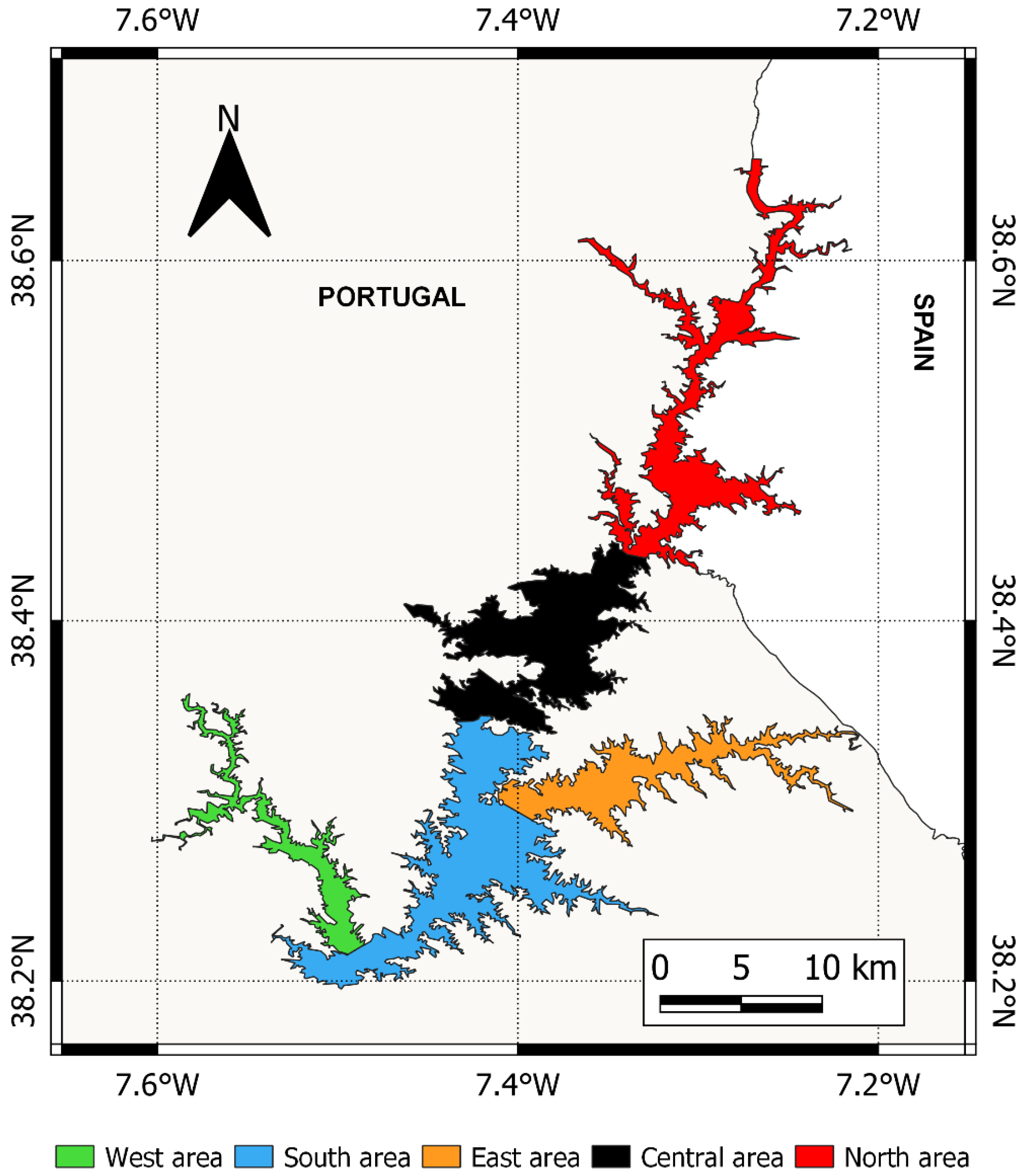
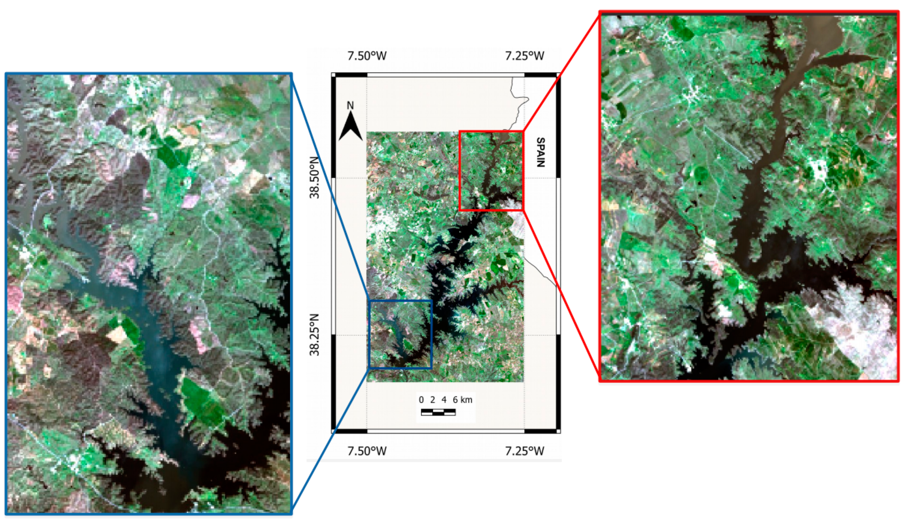
2.1. Area and Period of Study

The Alqueva reservoir (southeast of Portugal in Alentejo region) is the largest artificial lake in Western Europe, with a surface area of 250 km², 85 km length and a maximum depth of 65 m. Currently, the Alentejo region is an area with droughts that can persist for more than two years, and several months of low precipitation associated with very high maximum temperatures, between 25 °C and 45 °C (June to September). In this context, and with increasing water needs for human consumption, agriculture, and industries, the Alqueva reservoir constitutes a fundamental water resource in southern Portugal. The primary inflow to Alqueva is the river Guadiana (north of reservoir) bordered by Spain in the east. Temporal and spatial variations of water quality in the present study are analyzed in the Alqueva reservoir as a whole, and by five areas, the same used in the previous study [30] and shown in Figure 1. The period of study using OLCI data in this work comprises four years, between 2017 and 2020. However, the data used to define the empirical algorithms belong to different periods.

Table 1. Periods considered for each dataset used.

Data	Objective	Period
Sentinel-3/OLCI (Satellite data)	Estimate water quality and OWTs	2017–2020 (Period of study)
Surface reflectances (Satellite data and measurements)	Validation of OLCI surface reflectances	May 2016–September 2020
SD (Measurements)	Empirical algorithm	May 2016–October 2021
Chl-a/Turb (Laboratory data)	Empirical algorithms	July 2017–October 2021
PC (Laboratory data)	Empirical algorithm	February 2018–October 2021

shows the periods of all data used in this paper.

2.2. Sentinel-3/OLCI Data

The Ocean and Land Colour Instrument (OLCI) is a visible–near-infrared imaging spectrometer onboard the Sentinel-3 satellites launched by the European Space Agency (ESA). There is a constellation of two satellites: Sentinel-3A, launched in 2016, and Sentinel-3B, in 2018. OLCI will be widely used for studying the open ocean and inland/coastal waters since two more versions of the sensor are planned for launch over the next years (Sentinel-3C in the period 2023–2030 and Sentinel-3D in 2025–2032), thus allowing continuity. Since the launch of Sentinel-3B in April 2018, the Alqueva reservoir currently has a daily revisit. The instrument OLCI has a spatial resolution of 300 m (full resolution, FR) or 1200 m (reduced resolution, RR). Despite the spatial resolution of 300 m, it can be applied in large lakes, and due to its fairly high spectral resolution (21 bands in the range of 400–1020 nm), it is very useful for water and algae bloom monitoring. It also has a very relevant aspect in the study of lakes and oceans: sun-glint minimization [46]. With sun-glint minimization, the OLCI allows to include in the study practically all cloud-free days between May and August, months when deterioration of water quality and the emergence/evolution of microalgae must be monitored. With the Sentinel-2/MSI instrument, despite its better spatial resolution, many days would be excluded due to sun-glint presence, as discussed in a previous work [30].

The dataset used in this study is the Sentinel-3 Level-1 (top of the atmosphere), with 300 m spatial resolution (full resolution product) and was downloaded from Copernicus Open Access Hub (https://scihub.copernicus.eu/dhus/#/home, accessed on 1 November 2021). The OLCI Level-2 Water Full (300 m) and Reduced (1200 m) resolution products are also available as Level-2 (with atmospheric correction). However, Level-1 reflectances were used here in order to apply the suitable atmospheric correction scheme (Section 3.1) to obtain the surface reflectances.

2.3. In Situ/Laboratory Data

Since 2016, measurements of SD have been carried out at various points in the Alqueva reservoir. The SD is a quick and simple way to assess the transparency of water. It consists of a disk divided into four, with black and white contrast, and it is used to measure the depth until is visible in the water column. Generally, the lower the SD, the higher the Turb. During the period 2016–2021, the highest SD value was obtained on 11 March 2019, with 7 m measured at two locations in the Alqueva reservoir (south region). This maximum is much higher than the previous maximum of 5.5 m on 24 May 2017. The average value of all measurements in the Alqueva reservoir from 2016 to 2021 is 2.94 m. A minimum value of just 0.4 m was measured in August 2017 in the northern region of the reservoir. The lowest values of SD were measured during periods with presence of microalgae in the reservoir.

Since 2017, water samples and laboratory analyses have been carried out to have concentrations of Chl-a, PC, and Turb (Table 1). Water samples were collected at 0.5 m depth. Chl-a determination was based in molecular absorption spectroscopy and the equations developed by Lorenzen [47], according to the standard methods NP 4327:1996 [48] and EN ISO 10260:1992 [49]. Turb was determined using the nephelometric method [50]. PC determination was performed following the procedure proposed by Horváth et al. (2013) [51], extracted with phosphate buffer with the modifications suggested by Lauceri et al. (2017) [52]. The highest values of Chl-a/PC concentrations and Turb were obtained in late summer or early autumn (August/September), coinciding with microalgae blooms.

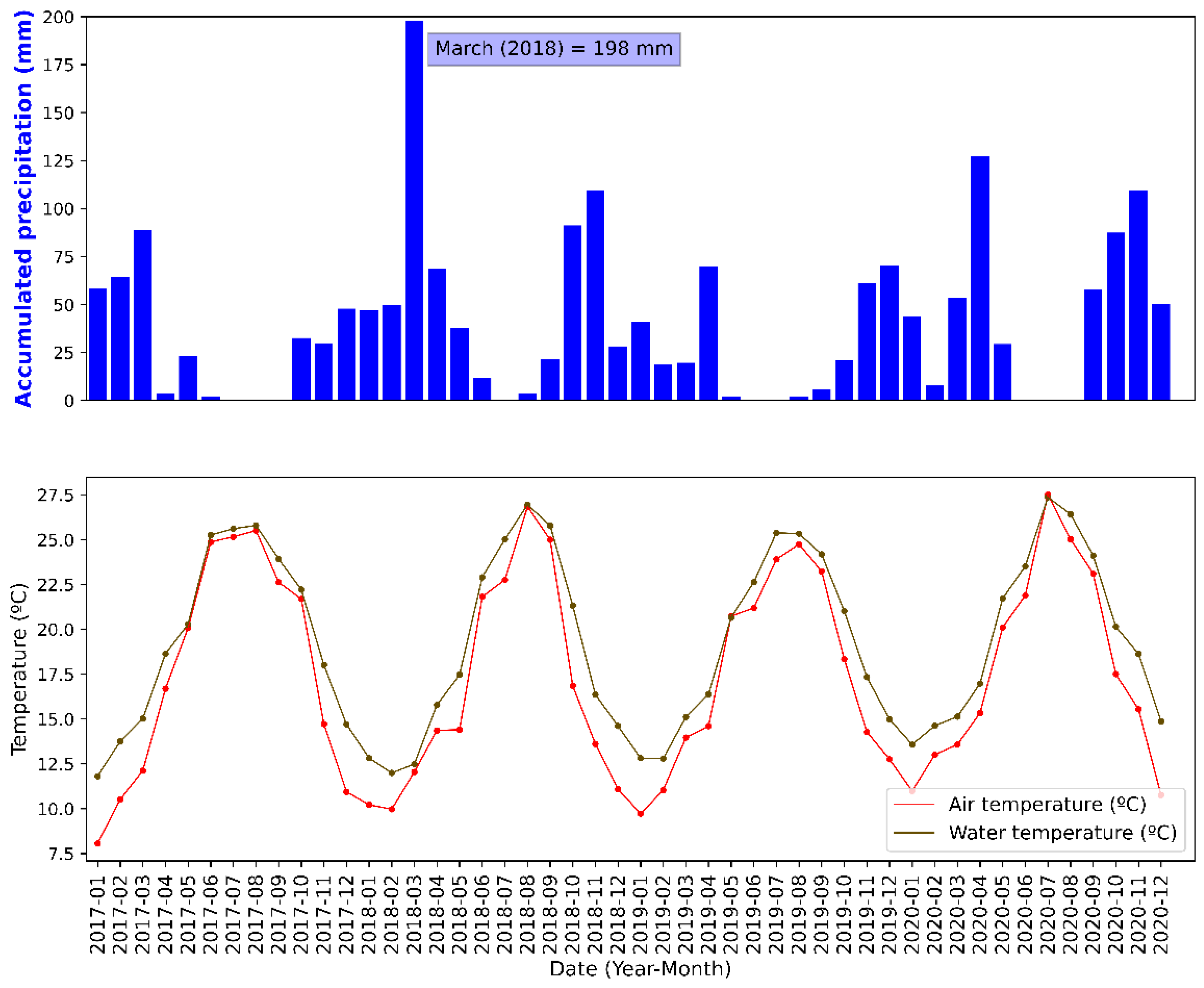
2.4. Meteorological Data

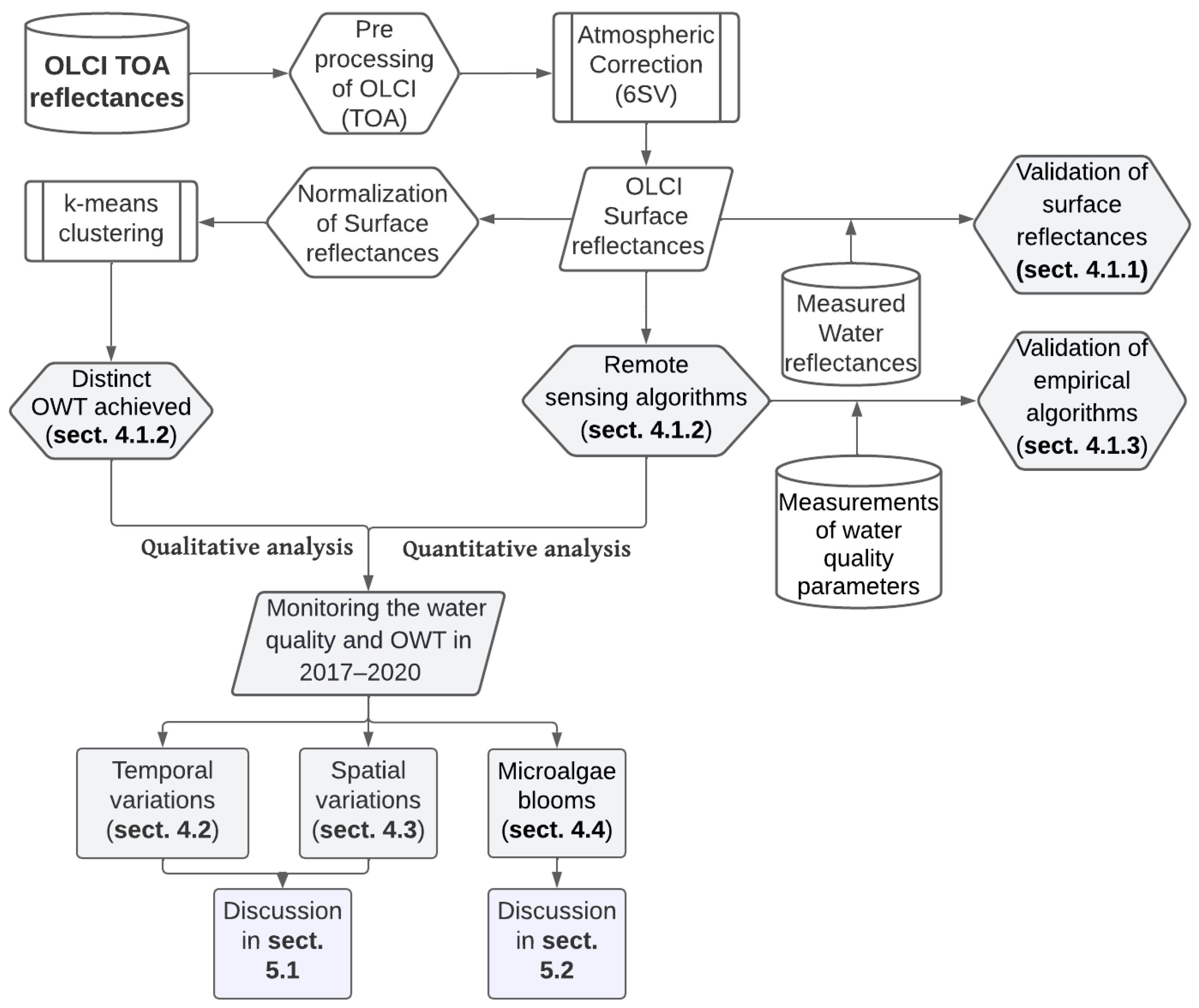
Since 2017, three stations were installed in the Alqueva reservoir, recording meteorological data with a temporal resolution of one minute, namely, wind intensity and direction, air/water temperatures, relative humidity, solar radiation, and accumulated precipitation, among other parameters. One of the stations is installed in a floating platform (Montante station), and the other two meteorological stations (CidAlmeida and Barbosa stations) are installed on the margins of the reservoir. The water temperature was measured on the Montante station at various depths, namely, at 0.05, 0.25, 0.50, 0.75, 1, 2, 4, 6, 8, 10, 12, 15, 20, 30, and 60 m depth. In the Alentejo region, where the Alqueva reservoir is located, the summers are very hot and dry, with high solar radiation. Between May and September, the average rainfall is very low, and this rainfall is mainly convective. Almost all the accumulated precipitation is recorded in the period between October and May. Wind intensity is normally of weak (or weak to moderate) intensity in the Alqueva reservoir [53]. Over the entire analyzed period, only in March 2018 was the average wind intensity above 4 m/s. Figure 2 shows the monthly evolution of meteorological parameters in the period 2017–2020: air temperature, water temperature, and monthly accumulated precipitation. The water temperature follows the variations of the air temperature but presents smaller differences between months due to its high heat capacity and thermal inertia.

3. Methodology

Satellite remote sensing of water quality parameters relies on the use of surface spectral reflectances above water. However, Sentinel-3 OLCI measurements are taken at the top of the atmosphere (TOA). It is thus necessary to atmospherically correct the data in order to account for the absorption and scattering atmospheric effects and obtain the surface signal. In Section 3.1, the atmospheric correction method and the empirical algorithms are described. The k-means approach implemented to define different optical water types is presented in Section 3.2. Section 3.3 shows the methodology followed in the comparative analysis between quantitative and qualitative estimations of water quality. Figure 3 shows a flowchart summarizing the methodology and main results of this work. The grey boxes show the main results, and in parentheses the subchapter is shown.

3.1. Atmospheric Correction and Empirical Algorithms

The satellite data of Sentinel-3/OLCI used are Level-1 (see Section 2.2) corresponding to TOA spectral measurements, which are subsequently corrected for the effects of the atmosphere in order to obtain the surface signal. Therefore, in order to obtain estimates of water parameters, the following procedures were carried out:

(i) 

The preprocessing of TOA Sentinel-3 imagery, including image reading, subset to Alqueva reservoir area, processing of radiances to reflectances, and extraction of the products. These four steps were performed using the toolbox SNAP (Sentinel Application Platform, http://step.esa.int/main/toolboxes/snap/, accessed on 1 November 2021), version 6.0. The top-of-atmosphere (TOA) reflectances were extracted from the OLCI images. The products SZA (solar zenith angle), SAA (solar azimuth angle), VZA (view zenith angle), and VAA (view azimuth angle) were also extracted, to be used in the atmospheric correction scheme as geometrical conditions.

(ii) 

The second step is the atmospheric correction of the various effects of the atmosphere, namely, ozone, water vapor, and aerosols. A reliable and adequate atmospheric correction process in the analysis of surface parameters in lakes or ocean is essential, as water usually has low reflectances, so small errors in the atmospheric correction can lead to large errors in surface reflectance estimates. In this work, the atmospheric correction method 6SV was assessed to obtain the surface reflectances, applied to cloud-free images acquired by the OLCI instrument. Python code was used to transform TOA to surface reflectances. Other atmospheric correction methods were verified in the literature, such as the ACOLITE or C2RCC (Case 2 Regional CoastColour) processor. We selected the 6SV method mainly due to three factors: (a) There are high correlations between estimated and measured reflectances in the Alqueva reservoir considering previous studies [30,44,45]. These high correlations mean that when using the 6SV method, despite the associated errors (in absolute value), there is similarity between shape of estimated and measured reflectances, being a crucial factor for a correct definition of OWTs. (b) It is a method that normally does not have null or negative reflectances, in situations of high water transparency (low surface reflectances), while with C2RCC and ACOLITE processors this happens. We tested the C2RCC processor for days with clean water, i.e., low water reflectances, and we obtained negative reflectances, without necessarily having high AOTs. This result for the Alqueva reservoir is in agreement with other studies, where there is an underestimation of the reflectances compared to the surface reflectances measured using the C2RCC processor [20,54]. (c) It is a method of atmospheric correction that has been extensively used in several lakes and with good accuracy compared to measured surface reflectances [21,22,23,30,44,45,55,56].

The 6SV is a vector version of the 6S (Second Simulation of a Satellite Signal in the Solar Spectrum), being a robust radiative transfer code that is highly accurate, and was also used in the previous study in the Alqueva reservoir [30]. The 6SV method is used to correct the OLCI images over the Alqueva reservoir, allowing to account for the various effects of the atmosphere. We used input parameters for the 6SV process to model the atmospheric effects and spectral/geometrical conditions, as shown in

Table 2. Input parameters of 6SV model applied to Sentinel-3/OLCI.

	Source	Parameters
Input type	Sentinel-3/OLCI	TOA reflectance
Geometrical conditions	Sentinel-3/OLCI	Solar zenith angle, solar azimuth angle (◦)
		View zenith angle, view azimuth angle (◦)
		Month, day
Atmospheric conditions (user)	Aeronet	Water vapor (g/cm2)
	Ozone Monitoring (OMI)	Ozone (cm-atm)
Aerosol model (type)	-	Continental
Aerosol model (concentration)	Aeronet	Aerosol optical thickness at 550 nm
Spectral bands	Sentinel-3/OLCI	Spectral function responses

.

The validation dataset of surface spectral reflectances was obtained at the Alqueva reservoir with a portable spectroradiometer FieldSpec UV/VNIR (ASD, Inc., Bouler, Colorado USA). More details about the FieldSpec UV/VNIR (ASD, Inc.) can be found in [57,58]. In addition to the correlation coefficient between in situ reflectances and satellite data, the bias, the MAE (mean absolute error), and MAPE (mean absolute percentage error) were used. The bias error and the MAE measure of the overall errors are that the MAE correspond to absolute errors. MAPE is defined as the mean of absolute differences between estimates (satellite-derived) and observations and measures the error in percentage terms.

The remote sensing algorithms obtained for the Alqueva reservoir were based on empirical relationships between the water quality parameters and Sentinel-3/OLCI retrievals of surface reflectances. In situ measurements of SD and laboratory analysis of Chl a, PC, and Turb were related to the atmospherically corrected surface spectral reflectances obtained from OLCI, through regression algorithms. Maximum differences of 1 day were accepted between water quality parameters and OLCI surface reflectances. In order to relate satellite data with measured/laboratory data, the nearest water pixel was used. An additional filter has been added to exclude pixels at the land/water boundary, the Modified Normalized Difference Water Index (MNDWI). This index evidences the open water features compared with NDWI (Normalized Difference Water Index) while efficiently suppressing land, vegetation, and soil noise [59]. Water pixel selection was performed considering an MNDWI index greater than 0.5. It was found that this index excludes not only many mixing spectra, but also pixels contaminated by cirrus and even light clouds visible by the RGB image and distinguishable in the reflectance spectrum (much less variation in the visible to NIR bands, comparatively to purely water pixels).

The defined regression algorithms were validated using different (independent) periods from those used to establish the algorithms. The period for the different water quality parameters is distinct due to different covering periods. Algorithms for PC and Turb were defined in the period 2018–2020 and 2017–2020, respectively. For these two water quality parameters, the validation period is 2021. For SD and Chl-a concentrations, the definition of the algorithms were in 2016–2018 and 2017–2018 respectively, and the validation period corresponds to 2019–2021.

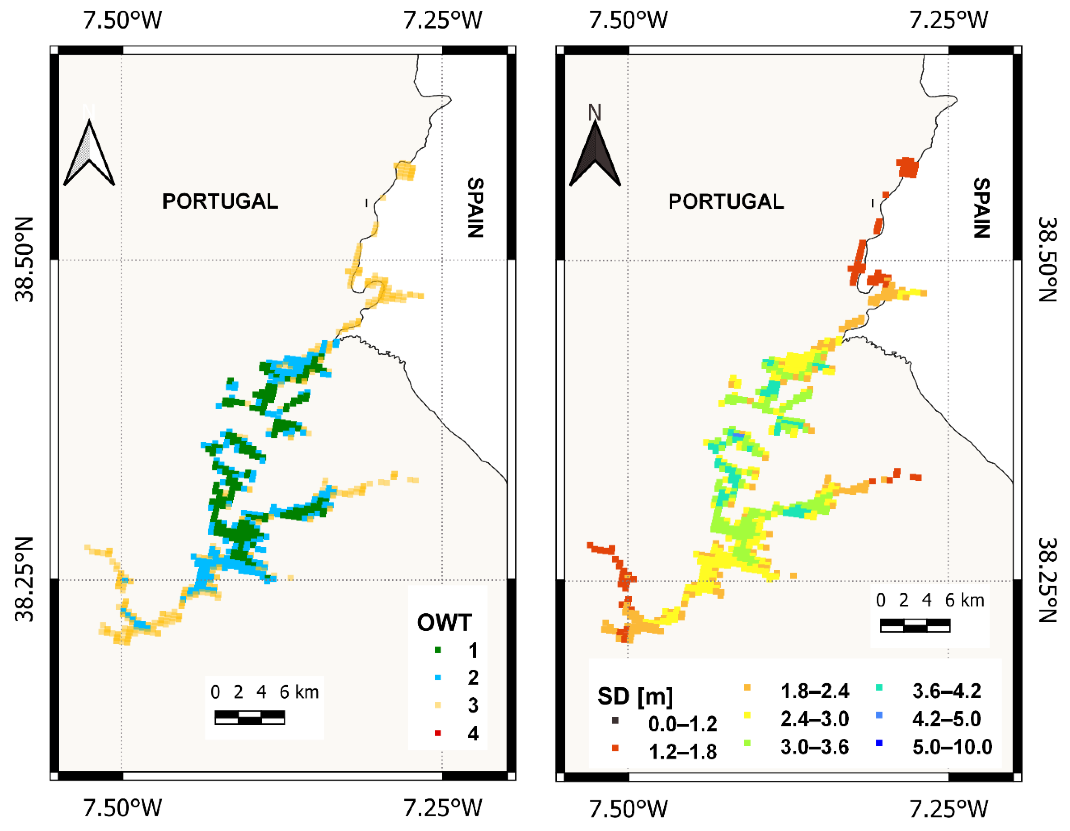
3.2. Definition of Optical Water Types (OWT)

Distinct optical water types (OWT) were identified based in the surface reflectance spectra of Sentinel-3 data in the period 2017–2020. Each type of OWT represents a group of similar optical characteristics and similar reflectance spectra. Prior to clustering, preprocessing was performed. It was applied to each day with clear sky over the reservoir, excluding pixels or days in the following cases:

➢

Days with at least one pixel having null values of view azimuth angle. These images represent days when the reservoir is at the limit of the OLCI image, thus having degradation in image quality and reflectance spectra.

➢

Pixels with MNDWI less than 0.5.

➢

Days when there are less than 200 pixels with MNDWI greater than 0.5.

➢

Days with at least one pixel with negative reflectance in one band between 490 nm and 708.75 nm. Only five days were excluded with this filter, being days with high AOT values.

After applying these four filters, all the water pixels were used to divide the spectra with similar characteristics within each of the clusters. The wavelengths chosen were in the range of 490 nm to 709 nm, that is, between band B4 and band B11 of the instrument OLCI.

K-means and fuzzy-c means, being unsupervised clustering methods, aim to cluster all input samples within different classes but require a priori selection of the optimal number of clusters and a method for excluding data from the analysis. Some studies identify very similar results between these two clustering methods [30,38]. The k-means approach was used, being one of the most popular non-hierarchical clustering techniques [33,34], as a method with high efficiency in the classification of large datasets [60]. Python code was used to run the k-means method and assign each of the OLCI pixels to a different OWT. The k-means algorithm was applied to the normalized OLCI reflectances instead of using the raw surface reflectances, to reduce the influence of the magnitude on the clustering and give greater relevance to the spectral reflectance shape [32,34]. Giving greater relevance to the shape allows absorption characteristics to have more impact on clustering. It also allows to reduce the effects of errors in atmospheric correction because these uncertainties have a greater effect on the amplitude of the spectra rather than their shape [32]. The normalization of each reflectance was made using its integrated value between B4 and B11 bands. This method was used because it does not give a greater weight to a defined part of the reflectance spectra, contrarily to other normalization methods. Unsupervised methods such as the k-means approach do not allow to exclude spectra from the analysis. In this way, this method may include spectra in a given OWT of pixels that are on the border between two or more OWTs. However, after processing the clustering method, some spectra could be excluded, through the information provided from the “silhouette width” [61]. The silhouette width measures how well each spectrum is clustered, having ranges between −1 to 1. A value of 0 of the silhouette width indicates that the spectra are on the boundary between two clusters and negative values indicate that those samples might have been assigned to the wrong cluster. In this work, only spectra with silhouette width above 0.05 were used. It was found that the silhouette index filter below 0.05 (pixel not assigned to any of the four clusters) excludes some spectra of doubtful quality (land/water mixture) that had not been excluded with the selection of MNDWI above 0.5. The silhouette width also allows to exclude spectra in areas that may have a mixture of two or more different OWTs. The silhouette width was also used to choose the statistically optimal number of clusters. The k-means method was run using two to ten clusters, and it was with four clusters that the highest mean silhouette value was obtained, that is, on average, the spectra are further apart spectrally compared to another selection of number of clusters.

3.3. Comparison between OWT and Water Quality Parameters

In order to have qualitative and quantitative estimations of water quality in the 2017–2020 period, the OWT classification was analyzed together with the estimations of water quality parameters. Aiming at full spatial cover and continuous monitoring of water quality parameters in the Alqueva reservoir, the atmospheric correction code 6SV was used to process all water pixels, for every cloud free day, obtained from Sentinel-3/OLCI (TOA) in the period. Filters were applied as explained in Section 3.2. The OWT classification allows assigning a cluster to each of the OLCI pixels, that is, an OWT spatialization map of the entire reservoir. The empirical algorithms provide, for every pixel, maps representing the estimates of water quality parameters. Then, the spatiotemporal variations of OWT and water quality parameters were analyzed, namely, Chl-a concentrations, PC concentrations, SD, and Turb. The silhouette index below 0.05 was used to exclude pixels, in addition to the MNDWI above 0.5. The water quality comparisons were performed based on boxplot representing the average conditions (average and median) and also the 10th, 25th (first quartile), 75th (third quartile), and 90th percentiles. The 10th and 90th percentiles were used to analyze the value corresponding to the 10% of highest and lowest severity for each water quality parameter. For the most correct comparison analysis between the OWT classification and water quality parameters, an intercomparison pixel-by-pixel (300 m of resolution) analysis was performed. The qualitative and quantitative comparisons were carried out by areas of the reservoir, dividing into the same five areas used in the previous study and presented in Section 2.1. The large differences in the number of OLCI pixels assigned to each Alqueva area would mean that analyzing the average characteristics of the entire reservoir would give greater relevance to the central and southern areas, possibly masking local variations in areas with much fewer pixels. In

Table 3. Daily average of pixels for each year and area.

	North	Center	South	West	East
2017	70	228	275	26	81
2018	70	227	282	27	85
2019	66	207	267	25	77
2020	47	172	237	20	62

, the daily average of pixels per area and per year is presented. This average of pixels (by year and by area) was calculated, counting the number of pixels of all OLCI images used in this study.

4. Results

4.1. Definition of Optical Classification and Empirical Algorithms

4.1.1. Validation of OLCI Surface Spectral Reflectances

In order to estimate water quality parameters and the OWT classification, it is first necessary to obtain the surface reflectances applying the atmospheric correction process, as explained in Section 3.1. The validation of OLCI surface reflectances (after applying the 6SV method) is shown in

Table 4. Statistical indicators between the measured and satellite-derived (OLCI) water reflectances using the 6SV method.

N = 27	Correl.	Bias	MAE	MAPE (%)
B4	0.92	0.006	0.006	39
B5	0.92	0.006	0.006	31
B6	0.96	0.004	0.005	18
B7	0.95	0.004	0.004	26
B8	0.94	0.003	0.003	31
B9	0.92	0.003	0.003	33
B10	0.92	0.003	0.003	29
B11	0.93	0.002	0.003	47

and corresponds to the period May 2016–September 2020. In the present study, only the surface reflectances between B4 band (490 nm) and B11 band (709 nm) were used, where correlations are higher than 0.9 (close to 1) and MAPE lower than 40% (except B11 band). The estimated values are overestimated compared to those observed (positive bias).

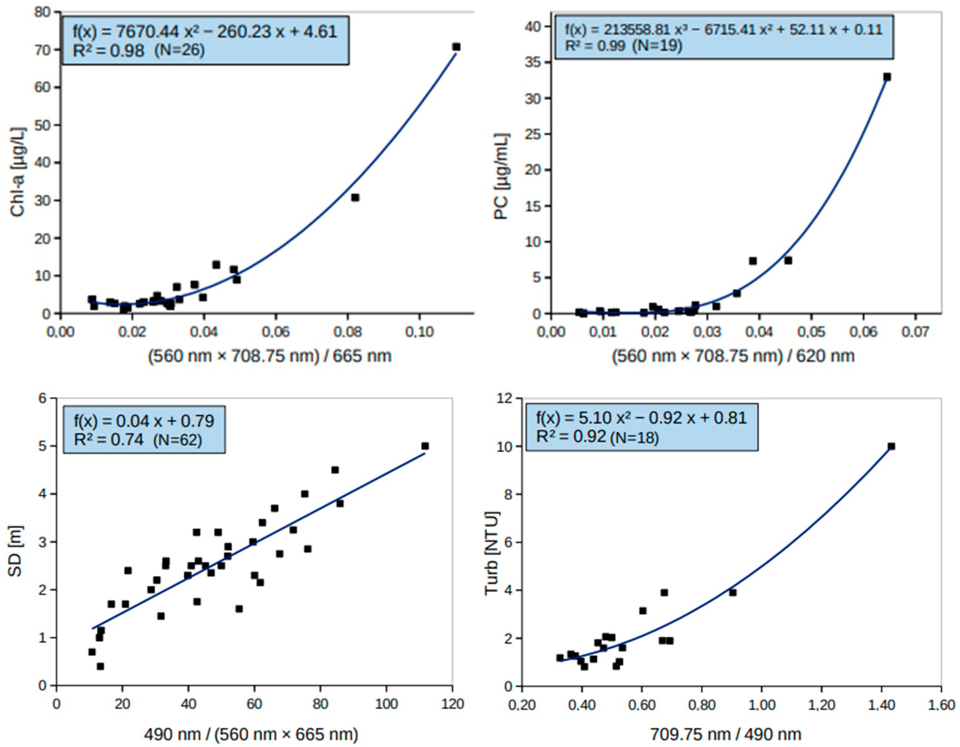
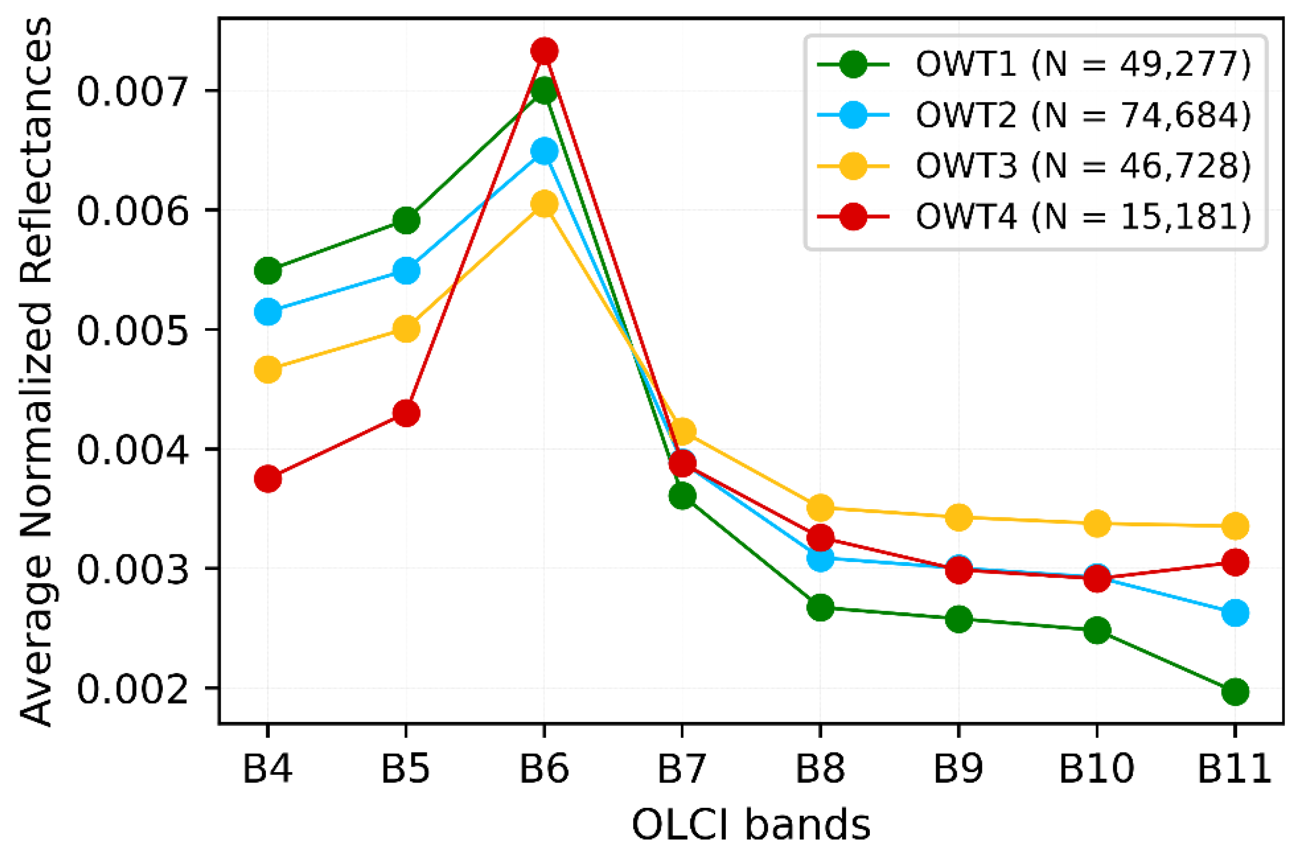
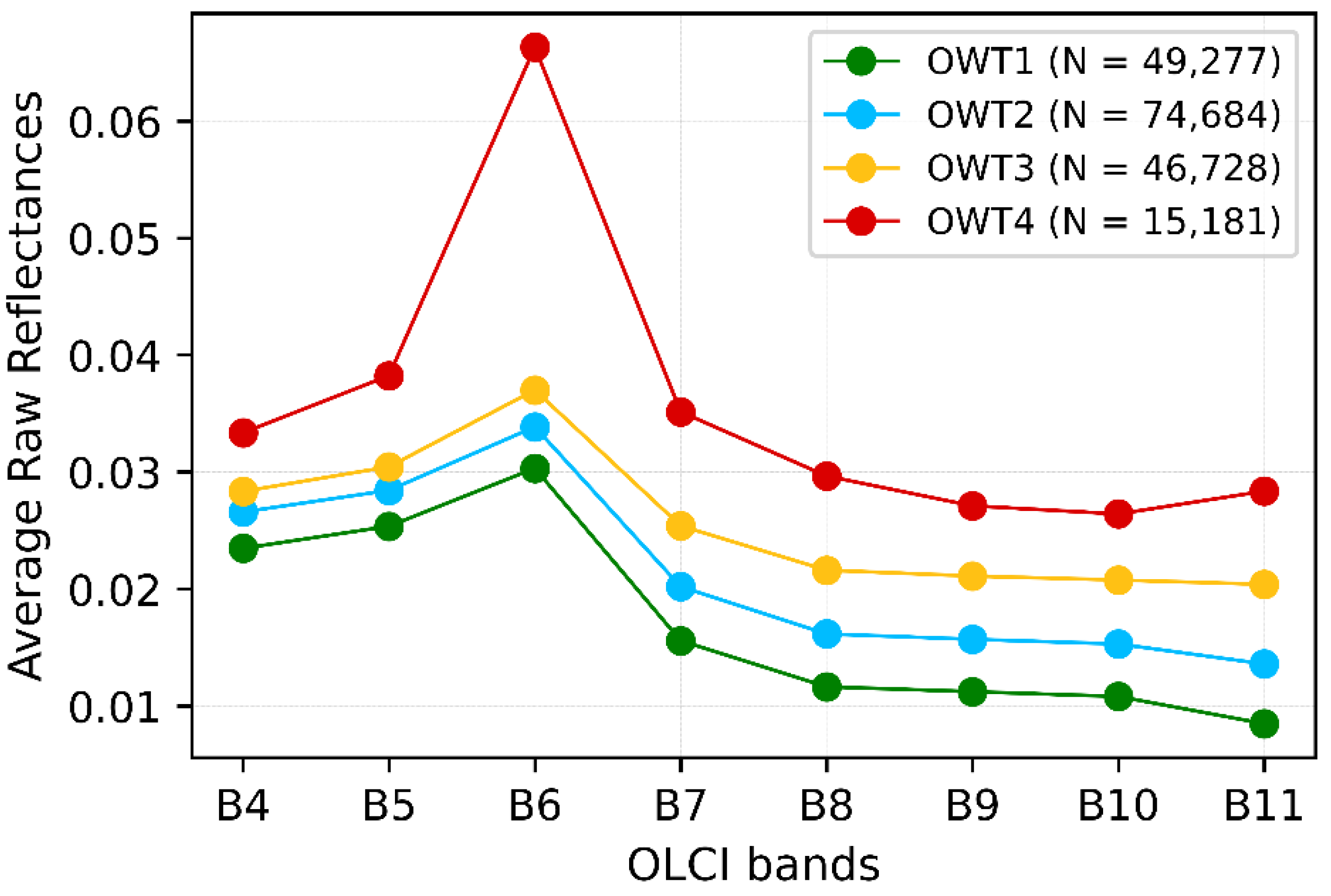
4.1.2. Definition of the Empirical Algorithms and the Four OWTs

Two independent methods were developed to estimate the water quality in the Alqueva reservoir: empirical algorithms for definition (Section 3.1), and using the k-means clustering method, four distinct OWTs were achieved (Section 3.2).

The best algorithm found for Chl-a, with the best results of R² and NRMSE, was adding the reflectance of the green band (560 nm) to the bands 709 nm and 665 nm. Normally, more than half of the year, Alqueva reservoir present low Chl-a concentrations. This fact helps to explain why the use of only red to NIR bands does not present good statistical results, widely used in the context of lakes [62]. The green band of 560 nm is a chlorophyll reference (chlorophyll minimum absorption), where the presence of greater reflectance represents greater Chl-a concentrations. The green band (560 nm in Sentinel-3 OLCI) is widely used in cases of lower Chl-a concentrations. The other two bands used in the algorithm (665 and 709 nm) are used in cases of high concentrations of Chl-a.

$$\mathrm{Chl-a}=7670.4\times {\left(\frac{B6\times B11}{B8}\right)}^2-260.23\times \left(\frac{B6\times B11}{B8}\right)+4.61$$

(1)

Although high concentrations of Chl-a are indicators for the appearance of cyanobacteria, they do not imply necessarily its presence. The pigment phycocyanin is a marker for cyanobacterial presence in eutrophic water and has an absorption peak at approximately 615–620 nm [18,19]. The PC algorithm determined with the best coefficient of determination uses this absorption peak ( of OLCI), as well as a near-infrared (NIR) band, centered at 709 nm (very low PC absorption) and also the green band ( of OLCI; medium absorption and high reflectance):

$$\mathrm{PC}=\mathrm{213,558.8}\times {\left(\frac{B6\times B11}{B7}\right)}^3-6715.41\times {\left(\frac{B6\times B11}{B7}\right)}^2+52.11\times \left(\frac{B6\times B11}{B7}\right)+0.11$$

(2)

The SD algorithm developed by Rodrigues et al. [30] for Sentinel-2/MSI is adopted in the present study, using instead Sentinel-3/OLCI. The equivalents OLCI bands are used here, adjusting the linear regression coefficients:

$$\mathrm{SD}=0.036\times \left(\frac{B4}{B6\times B8}\right)+0.79$$

(3)

The Turb algorithm, determined with the best coefficient of determination, uses bands $B4$ and $B11$, presenting the following equation:

$$\mathrm{Turb}= 5.10\times {\left(\frac{B11}{B4}\right)}^2-0.92\times \left(\frac{B11}{B4}\right)+0.81$$

(4)

The scatter plots, with the best fit for each algorithm between satellite-retrieved reflectances and water parameter data, are shown in Figure 4 (chlorophyll a, phycocyanin, SD, and Turb).

Four distinct sets of reflectance means were defined (Figure 5). These reflectance means form the OWT classification in the Alqueva reservoir, which are representative of the averaged conditions caused by the optical properties of the water column. In addition, the median for each of the clusters was also calculated and showed very identical spectra for the different selected clusters (not showed here). The OWTs were organized in ascending number (1 to 4) based on ascending water turbidity of the water.

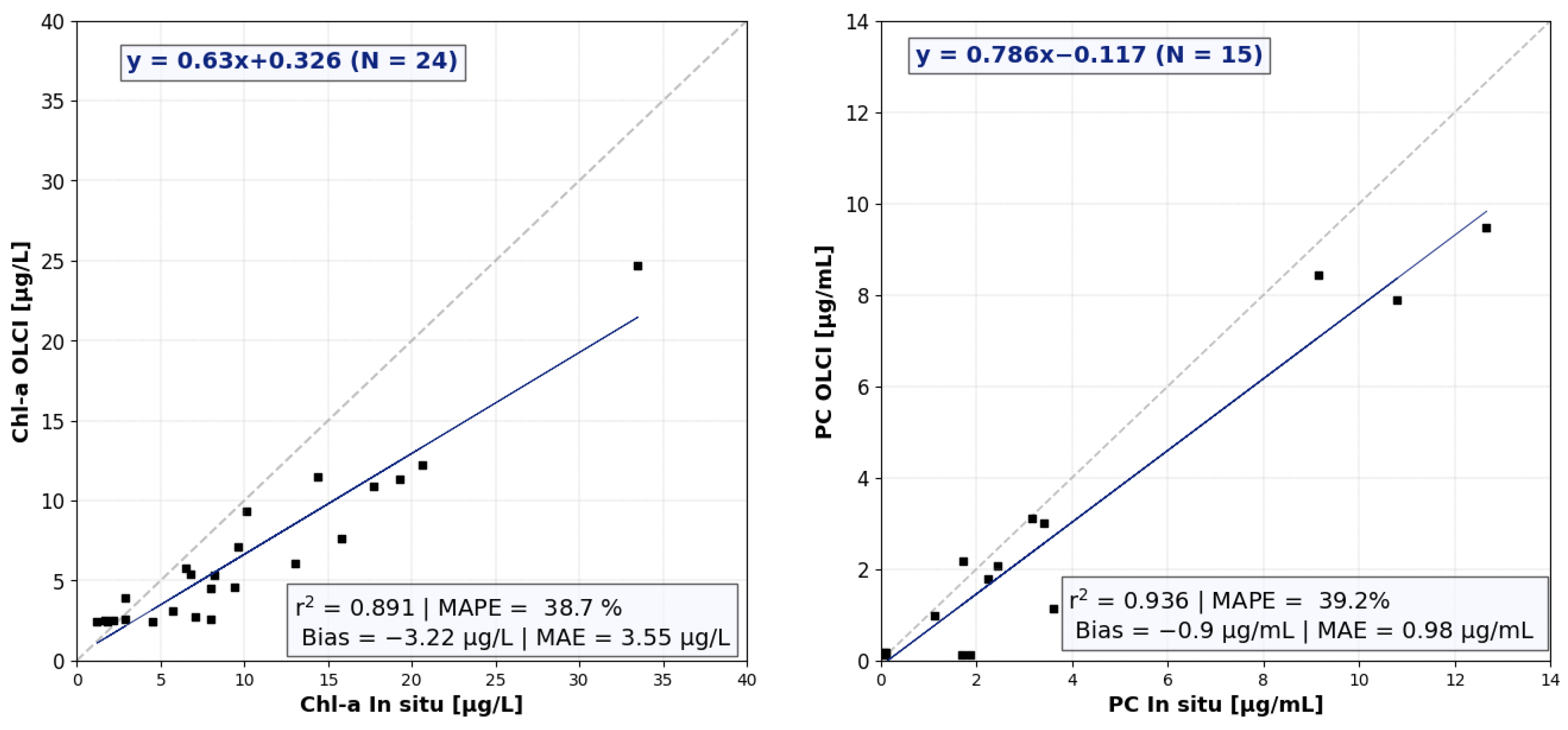
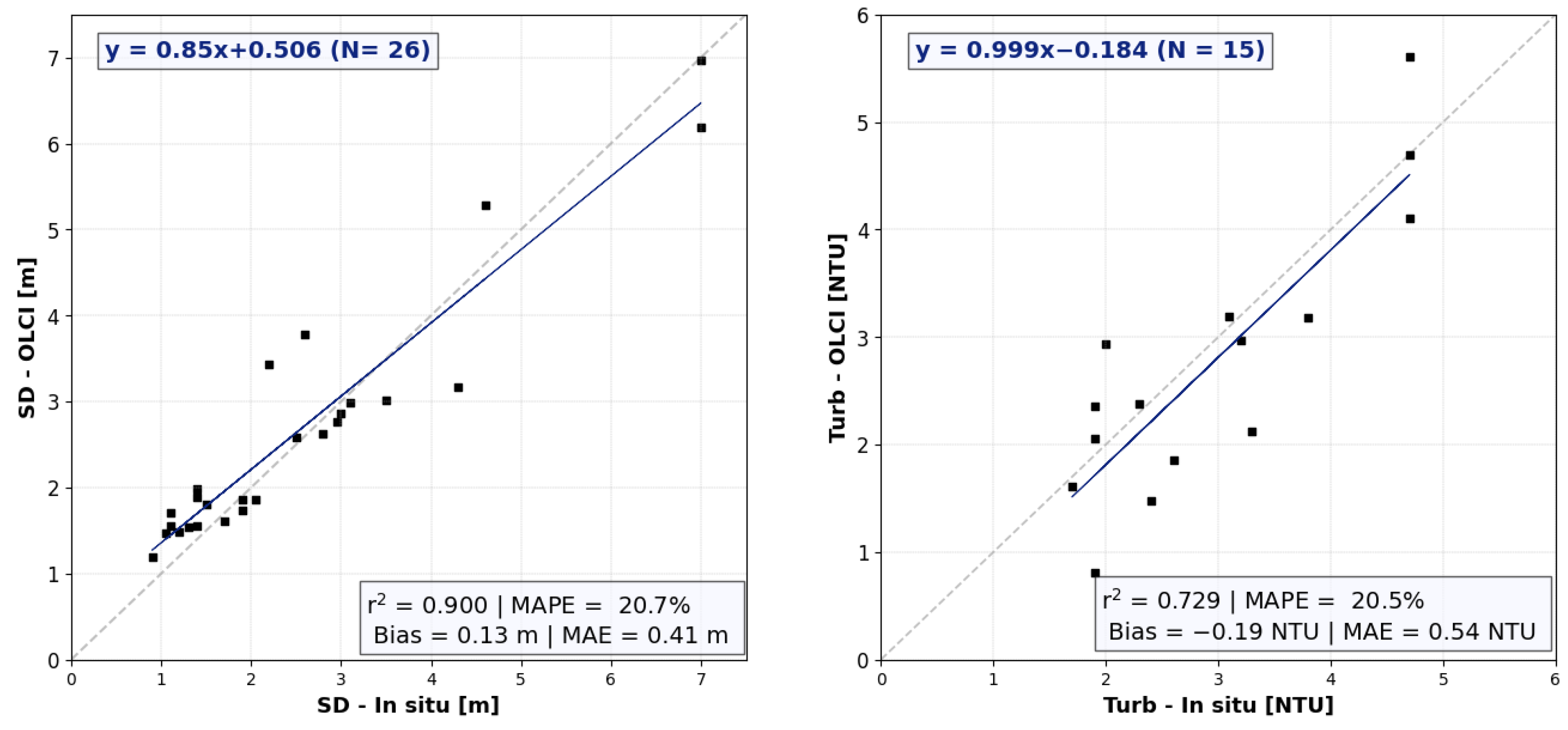
4.1.3. Validation of Empirical Algorithms

The results obtained using the developed empirical algorithms were compared with in situ measurements (validation of the empirical algorithms) for a different period with respect to that used to derive the four equations (Section 4.1.2). These algorithms were applied to the nearest water pixel with respect to the sites where the water samples were collected (Turb, Chl-a, and PC) and to SD measurements. In Figure 6, the relationships between estimated water quality parameters and the corresponding data measurements are shown.

In the validation of empirical algorithms (Figure 6), note the good agreement between observed and satellite estimates, with high coefficients of determination (above 0.9), except for Turb, with r² of 0.73. There are MAPEs close to 20% for SD and Turb, and 39% for Chl-a concentrations. Note that the MAPE near 40% in the validation of PC algorithm is also due to the fact that, in general, there are many low values of PC concentrations than higher values. Therefore, for very low PC concentrations, there can easily be obtained absolute mean errors in percentage above 100%. For SD and Turb, there is no relevant trend of overestimation or underestimation of the estimated data in relation to the measured data (bias close to 0). For Chl-a and PC, there is almost always an underestimation of the estimated data relative to the laboratory data, with negative bias (bias practically equal to the MAE), and almost all are points below the y = x line.

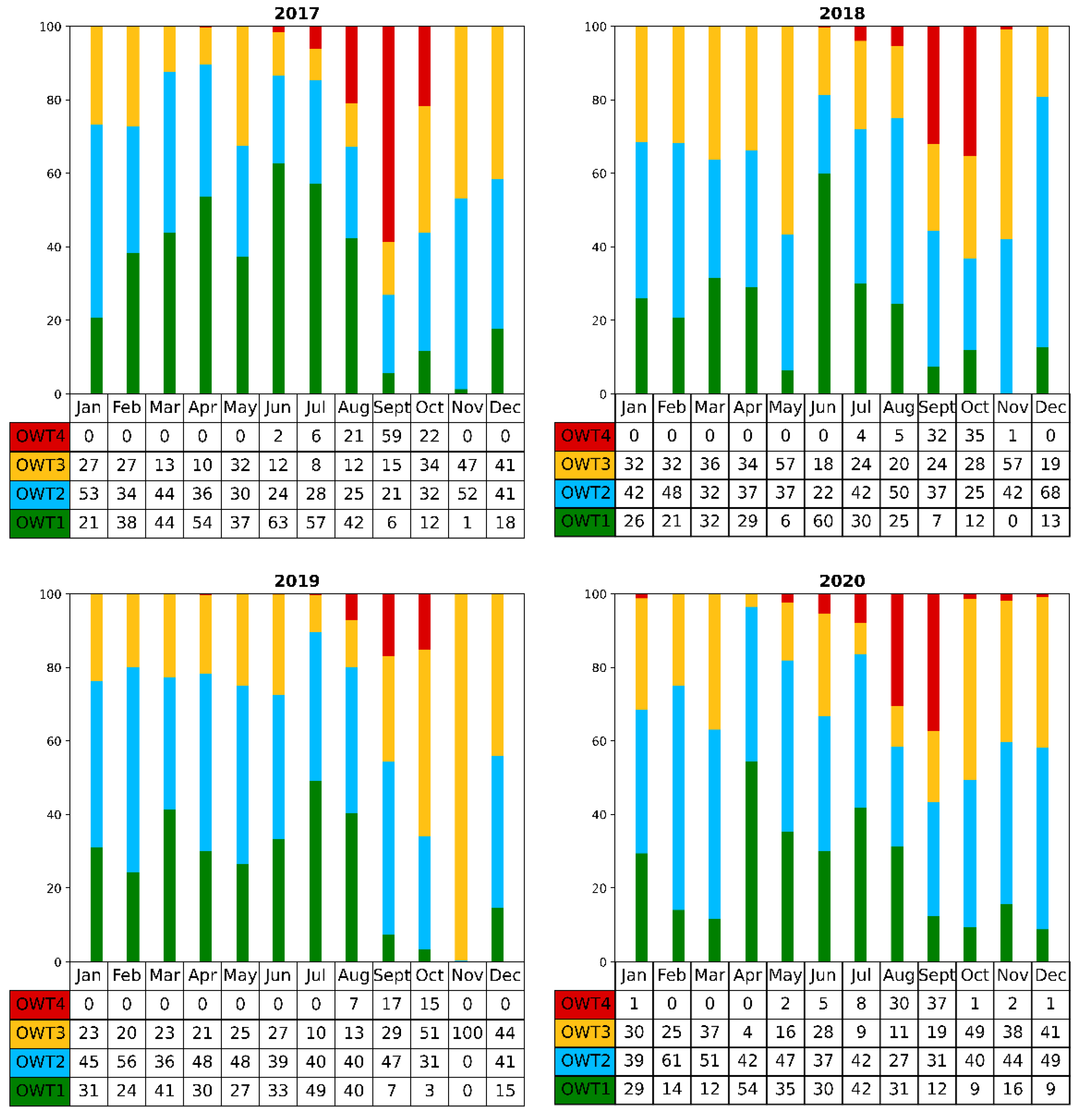
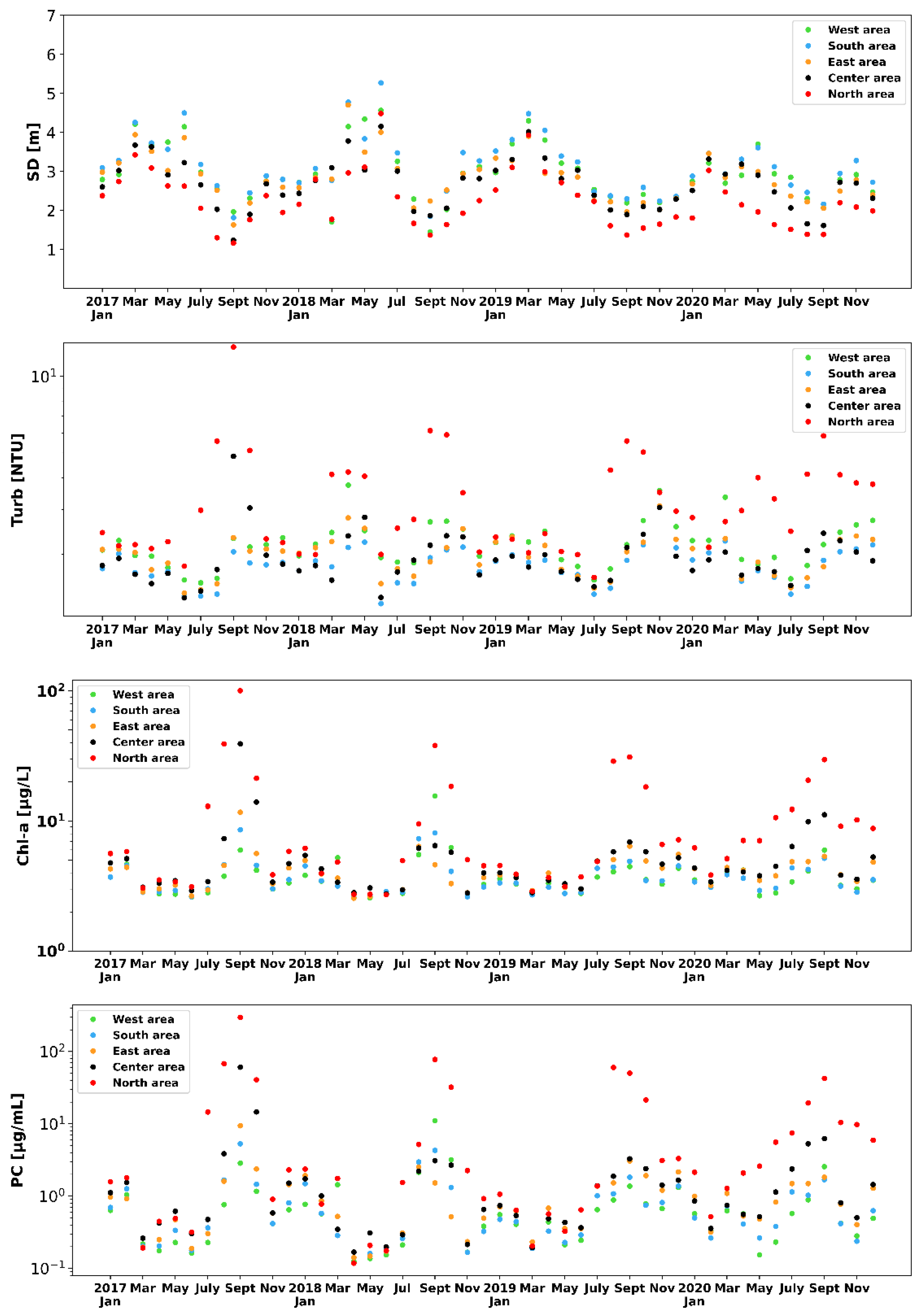
4.2. Qualitative and Quantitative Analysis of Water Quality

The clustering approach presented in this study (Section 3.2) has the advantage to differentiate subsets based mainly on the shape of surface reflectances. Four optical water types (OWT) were defined through a k-means approach applied to OLCI surface reflectances during the 2017–2020 period. The differences along the spectra of surface reflectances denote different optical characteristics and the predominance of one over another in water constituents (e.g., phytoplankton or non-phytoplankton particles). One of the essential features of spectral analysis is the verification of the variation between blue and green bands. Greater differences between band B5 (or other blue band) and band B6 represent greater presence of Chl-a (the greener the water is, the greater the reflectance of the green band in relation to the blue band). In the context of monitoring water turbidity, for minor ratios between reflectances in the blue and the red/NIR bands, greater water turbidity is expected.

Figure 7 shows the average raw reflectances (non-normalized) for each of the OWT groupings using the normalized reflectances. The typical spectrum of the OWT1 cluster (Figure 5 in Section 4.1.2 and Figure 7) represents conditions of low turbidity, that is, less dispersion and absorption by particles contained in the water. In the comparison between the typical conditions of the OWT1 and OWT2 cluster (Figure 5), a smaller difference was identified between the normalized reflectances (average) in the blue bands (B4 and B5 of OLCI); nevertheless, in the red and NIR bands (band B7) the cluster OWT2 overcomes the OWT1. Therefore, the areas assigned to the OWT2 cluster will normally have greater turbidity than areas assigned to the OWT1 cluster and weak or non-existent presence of microalgae. Analyzing the slope between the green (B6) and red (B7) band, it is identified that the OWT3 cluster represents the optical conditions with the highest absorption of the non-phytoplankton particles (sediments, for example). It is noted that the clusters OWT3 and OWT4 represent the most turbid optical waters, because in these clusters, on average, there are lower differences between the blue and red/NIR bands. The main source of turbidity in OWT3 is non-phytoplankton particles, while for cluster OWT4, it is the presence of microalgae, because this cluster represents areas with high concentrations of Chl-a. Another typical characteristic of the presence of microalgae in OWT4 is the peak at 708 nm, which is usually associated with high algae particle concentration [17,63].

The water quality algorithms and the OWT class through k-means clustering method (Section 4.1.2) were applied to all water pixels in the period 2017–2020. Therefore, a complete water quality characterization is obtained for all clear sky days, excluding pixels and days in the conditions defined in Section 3.2.

Figure 8 show the monthly evolution of Chl-a, PC concentrations, SD, and Turb obtained with the algorithms presented in Section 4.1.2 (Equations (1)–(4)). Each boxplot is composed of the mean, median, 25th percentile (1st quartile), 75th percentile (3rd quartile), and 10th/90th percentiles. In these graphs, the red bars represent the months (August to October) that normally have the highest presence of microalgae in the Alqueva reservoir. The frequency distribution of the four OWTs in the 4 years analyzed is shown in Figure 9.

Three main characteristics are presented and described below. The first is related to the presence of microalgae blooms in the reservoir in late summer and early autumn. The second is the high turbidity resulting from the overturn period. These two periods of greater turbidity occurred sequentially in the 4 years analyzed, having generally occurred between August and November. Finally, there is verification that in the rest of the months there are low Chl-a/PC concentrations and high percentage of OWT1 or OWT2 attribution.

(1) There is worse water quality in the months between August and October, associated with the presence of microalgae in the Alqueva reservoir. This fact can be seen with the identification of OWT4 pixels (Figure 9) and even higher values of Chl-a/PC concentrations (Figure 8). It is identified that the OWT4 cluster is practically present only in this period, associated with the appearance of microalgae. In three of the four years analyzed, the worst month in terms of water quality was September, with the highest presence of OWT4 pixels (in frequency), greater turbidity, and highest Chl-a/PC concentrations (Figure 8).

In the four years analyzed, September of 2017 is by far the month with the highest presence of microalgae in the Alqueva reservoir:

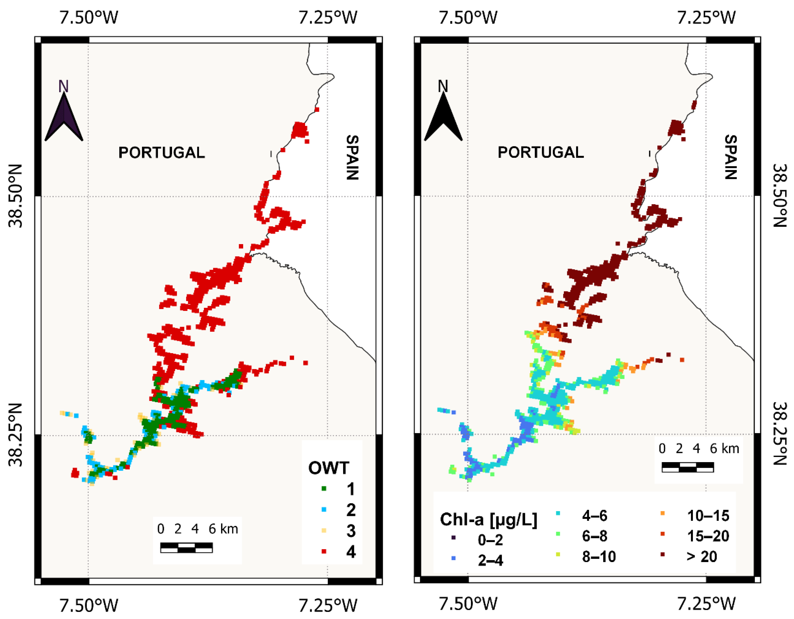
• 58.3% of the pixels in the entire reservoir presented the OWT4 classification. September 2020 had the second highest attribution to OWT4 cluster with 37.1%.
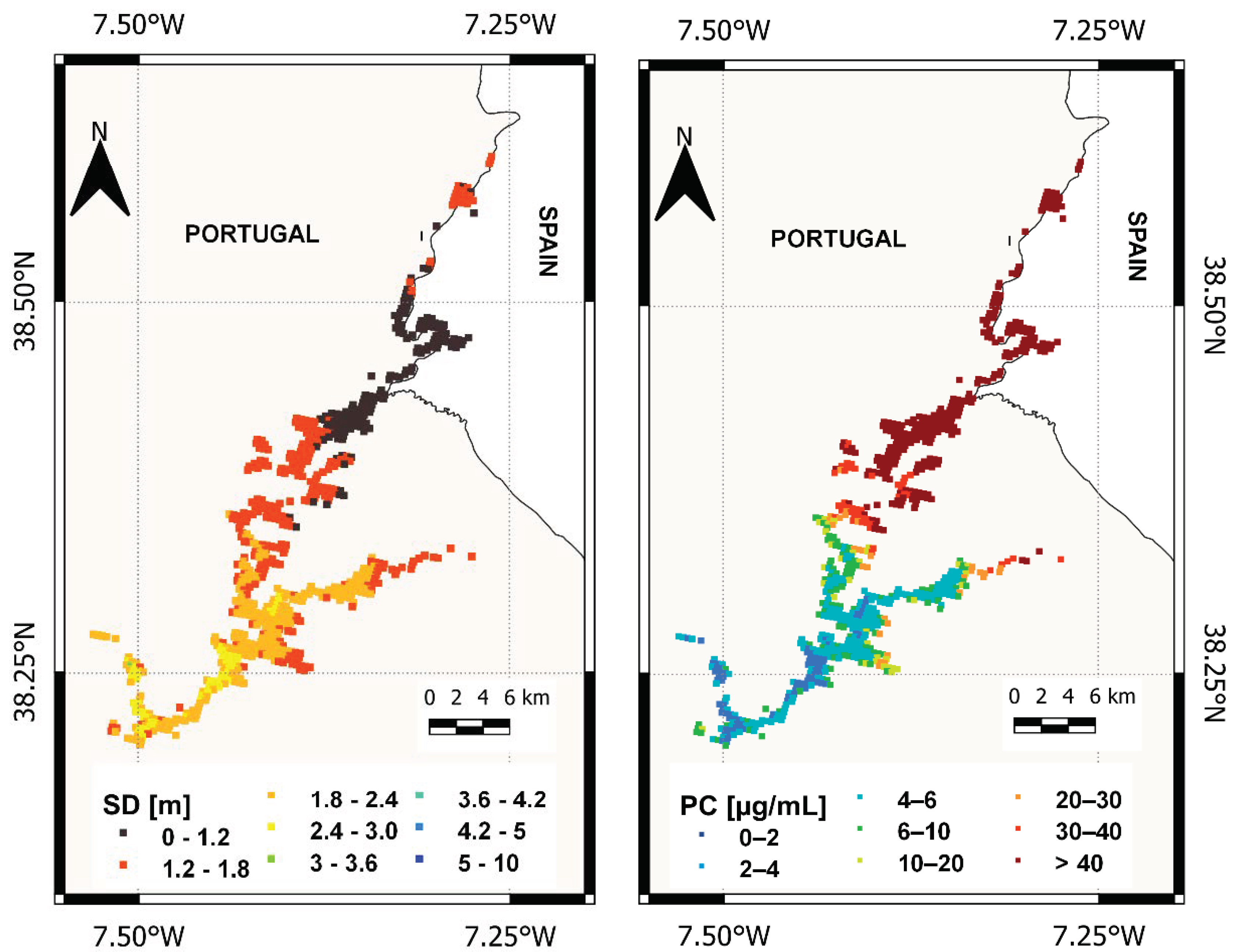
• Water quality estimates in September present the highest values of biomass load (higher Chl-a concentrations), a greater presence of cyanobacteria (much higher PC concentrations than any other month) and Turb, and lower SD. A highlight is the value corresponding to the 90th percentile for an SD of less than 2 m, which denotes a very high turbidity in practically the entire reservoir and in all the days available for analysis.

Therefore, there is a clear sign of deterioration in water quality in September, with the results obtained from two distinct and independent methodologies (OWTs analysis and the use of empirical algorithms) giving the same indication. It is important to highlight the very relevant differences between the 75th and 90th percentile (as well as the difference between the mean and median) for Chl-a and PC concentrations in all the months of September of the 4 years, mainly in September 2017 (Figure 8). This fact denotes that the upper extremes of Chl-a and PC are very far from the median/average value of the entire sample. As will be explained in Section 4.3, this is related to the large spatial disparities in the reservoir.

(2) Every year, the phenomenon of the overturn occurs in the reservoir, associated with the cooling of the surface temperature, leading to the mixing between layers from surface to the bottom. In recent years, the overturn has mostly taken place in the end of November. Except for the year 2020 (when the overturn took place in December), it was in November that the highest turbidity values in the reservoir have been identified, caused by non-photosynthetic particles (not associated with the presence of microalgae). That is,

• Lower frequency (%) of spectra (OWT1) associated with the most transparent water.
• The month with the highest frequency (%) of pixels assigned to the OWT3 cluster, representative of pixels with high turbidity.

In November 2019, only one OLCI image was used for the monthly analysis of OWT and water quality parameters. In this month, the overturn was identified as happening between early and mid-November. The temperature profile was determined by measuring the water temperature at various depths (Section 2.4), from surface to the bottom (60 m depth). In mid-November the reservoir was fully mixed and the overturn was concluded, i.e., a homogeneous temperature profile was found throughout the water column (Figure 10). The only day (15) used in this month is precisely the day before the completion of the overturn. From the sample of 639 pixels used, 99.7% of these (Figure 9) were assigned to the OWT3 cluster.

In 2020, the overturn occurred in December, and it was the second month with the highest frequency of OWT3 pixels in this year.

(3) Most of the months present low to moderate values of Chl-a concentrations (range of 0–8 μg/L) and low turbidity. These months also present a frequency greater than 60% of all pixels assigned to clusters representing the best water quality, that is, with the attribution of OWT1 and OWT2 class. In the period between January and August, only in August 2020 was there an exception, with less 60% of the pixels assigned to the OWT1 and OWT2 cluster. There are a few months with the allocation of (OWT1 + OWT2) close to or greater than 90% of all pixels analyzed for each of those months. These are the months of March/April (2017), June/July (2017), July 2019, and April 2020. It can then be concluded that there are representative pixels of lower water turbidity and lower Chl-a concentrations in winter months (except December), spring, and early summer months. The influence of runoff in water turbidity is a fourth aspect that will only be analyzed in chapter 4.4, as it was only relevantly identified in narrower areas of the reservoir. This is also evidenced in the reflectance spectra, that is, in the OWT classification.

A pixel-by-pixel intercomparison was also carried out in order to find relationships between the results of the water quality algorithms and the OWT attribution. To summarize the relationship between the four clusters and the parameters of water quality, four graphs are presented (Figure 11).

The water quality estimates from empirical algorithms generally present results in agreement with those expected for each of the clusters. That is, the typical values of Chl-a/PC concentration increased and SD decreased from OWT1 to OWT4. In the pixel-by-pixel intercomparison, a very significant number of points assigned to the OWT1 classification showed very low Chl-a/PC concentrations, and very low Turb. On the opposite side, almost all the pixels assigned to the OWT4 cluster presented estimates of very high Chl-a/PC concentrations and high Turb/low SD.

Table 5. Summary of key findings from the four defined OWTs. Water turbidity and Chl-a concentrations increase from cluster OWT1 to OWT4.

OWT Type(s)	Summary
OWT1	Characteristic of more transparent water spectra with lower Chl-a concentrations, and no presence of PC
OWT1 + OWT2	Characteristic of high water transparency
OWT2	OWT2 typically with lower water transparency and higher Chl-a concentrations than OWT1
OWT3 + OWT4	Water with low/moderate water transparency
OWT3	Low to moderate water transparency, but not necessarily associated with microalgae blooms
OWT4	High or very high Chl-a concentrations; microalgae blooms and risk of cyanobacterial presence

presents the main conclusions for each of the defined clusters.

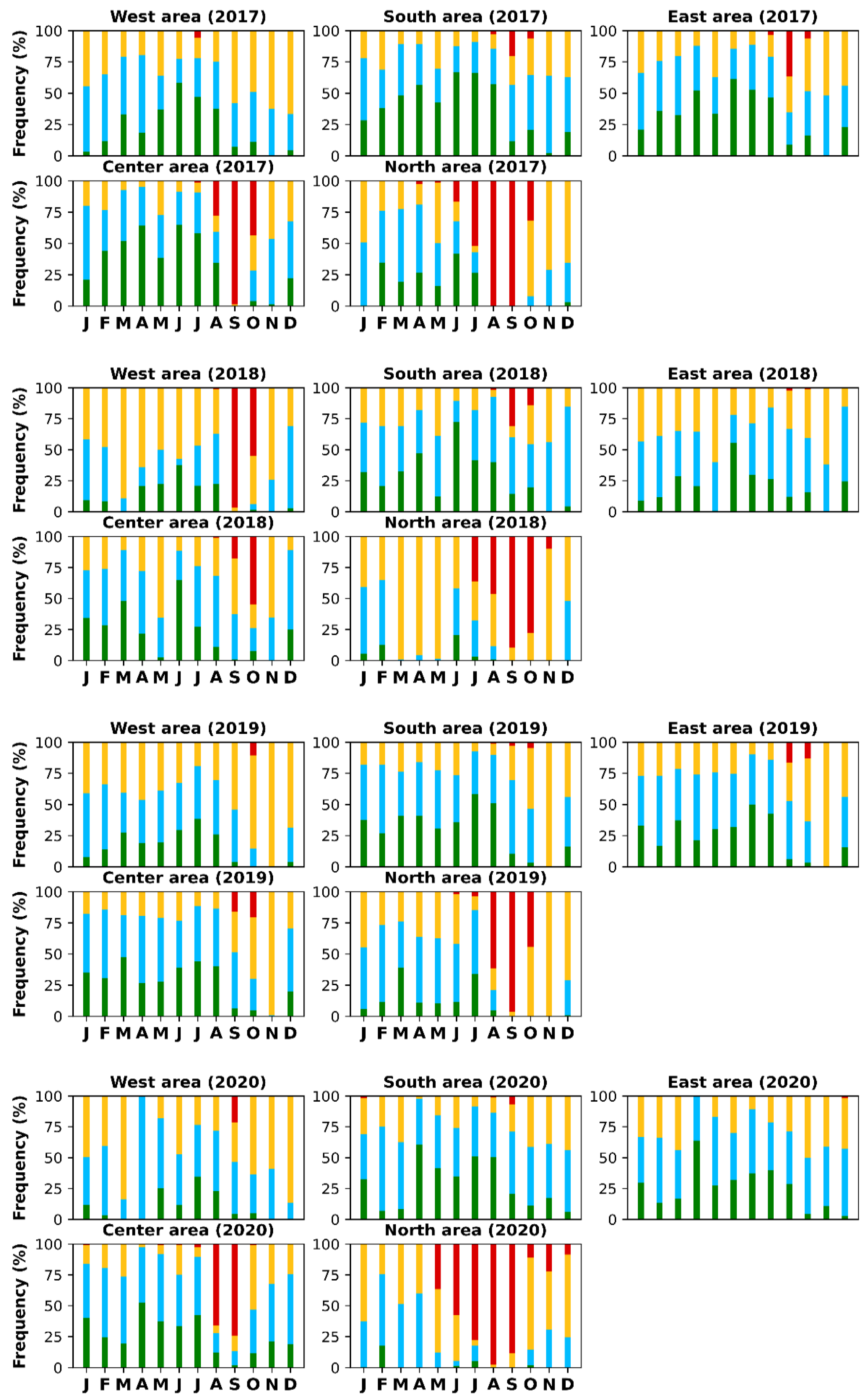
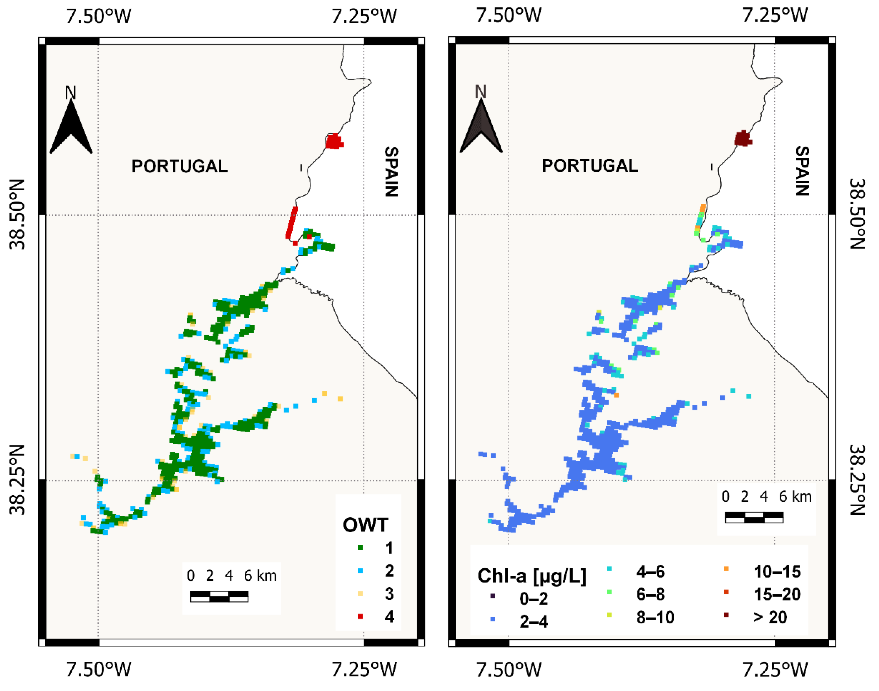
4.3. Spatial Variations of the Optical Water Types and Water Quality

In order to verify spatial variations, the reservoir was divided into five areas, calculating the OWT frequency for each month and area (Figure 12). Figure 13 shows the water quality mean by area and by month for the period 2017–2020. Spatial variations of OWT and parameters of water quality were analyzed, evidencing the following differences between the five areas of the reservoir:

• The northern area of the reservoir represents the area with the highest percentage of pixels assigned to OWT3 cluster or OWT4 during the four years analyzed. It is the area of the reservoir most affected by microalgae blooms (between July and October) and also by runoff phenomena after heavy rainfalls.
• The central area, being much wider than the northern area and further away from the Guadiana river inlet (in the north region), presents better water quality in all analyzed years compared to the north area. Precipitation and runoff affect this area less. However, microalgae blooms also disturb this area, mainly in the period between August and October, being the second area with greater deterioration of water quality in this period. This is verified not only by the analysis of OWT frequencies, but also by the estimates of Chl-a and PC concentrations.
• The southern area, one of the areas farthest from the area with the worst water quality (north area), presents, on average, the best conditions (lowest water turbidity and highest frequency of OWT1 + OWT2 pixels) of the entire reservoir. It also has the lowest impact of runoff effects or microalgae blooms.
• The western area (branch that starts in the south area towards the west/northwest) presented the most discrepant behavior in the 4 years analyzed, with respect to the July–October period, compared to the average of the entire reservoir. It was the area with the lowest frequency of pixels assigned to the OWT4 cluster in 2017, in the months with the presence of microalgae, being in 2018 the second worst (highest frequency of OWT3 + OWT4) area with high frequency identification of OWT3 pixels, in the month with highest rainfall (March 2018).
• The east area, despite being much narrower than the central and south areas, generally presents similarity to these two areas in relation to the frequency of OWT1 and OWT2. This area is also less representative of microalgae in 2018 and 2020, i.e., it presents lower frequency of pixels with OWT4 attribution and lower Chl-a/PC concentrations.

It is generally noted that in months without high rainfall and/or without the presence of microalgae (July to October mainly), a similar frequency of characteristic low turbidity spectra (OWT1 + OWT2) is observed between the four areas in the reservoir (except the north area). However, in these periods, the percentage of pixels assigned to the cluster featuring greater water transparency (OWT1) differs significantly between areas, being more significant in the south, center, and east areas. The north area is by far the one with the lowest frequency of OWT1 pixels. In this area, in 2020, there was no month with frequency higher than 20% attributed to the OWT1 cluster. In 2018, only June exceeded the 20% of pixels classified as OWT1, and in several months it did not even reach 0.1%. In 2018, the northern region of the reservoir presents 8 of 12 months with more than 85% of the pixels associated with either OWT3 or OWT4. Of these eight months, this area presents 4 months with practically 100% of the pixels attributed to the OWT3 cluster, representing turbid water. Of these four months, three coincide with high rainfall in the Alqueva reservoir and the other with the overturn phenomenon (November).

4.4. Extreme Events (Microalgae Blooms and Runoff after Heavy Rainfall)

The situations identified with the greatest spatial variations in the reservoir are related to intense precipitation events and microalgae blooms. In spring 2018 there was high rainfall, especially in March, with an accumulated value close to 200 mm at the CidAlmeida station (much higher than the average monthly precipitation). In a large reservoir, water quality varies more slowly than in a small reservoir. This can explain why March 2018 does not present high percentage of pixels associated with the OWT3 cluster in the entire reservoir (Figure 9). However, locally (in narrower areas) there is a significant increase in characteristic spectra of high turbidity, that is, associated with the OWT3 cluster. For the same month, the northern and western areas of the reservoir present 99% and 89% of the OWT3 class, respectively (Figure 12). These results are further corroborated by the RGB image obtained from the Sentinel-2 on 26 March 2018, identifying a brown color in north and west areas (Figure 14). This increase in water turbidity in the northern and western areas is identified by two methods of estimating water quality: OWT classification and water quality parameters. Figure 15 shows the maps of OWT and SD on 27 March 2018. The SD map is obtained by applying the algorithm (defined in Section 4.1.2) to all water pixels. In the central region, most pixels are assigned to the OWT1 cluster (blue pixels) with associated high water transparency (SD greater than 3 m). In the northern and western areas, practically all the pixels are assigned to OWT3 cluster, that is, representative of low to moderate water transparency. It is also in these two areas that the lowest values of SD are verified, with SDs normally below 2 m. On the frontier between the highest (OWT1) and lowest water transparency (OWT3) pixels, there are some intermediate water transparency (OWT2) pixels (blue pixels) with SDs around 2.5 m. There is a strong agreement between the brownish color in the RGB image (Figure 14) with the reduced SD and the OWT3 attribution (Figure 15).

During microalgae bloom events (July–October), there is also agreement between RGB images and water quality estimates (not shown here). Greenish colors in the RGB image (representing microalgae in water surface) correspond, in most cases, to the attribution of OWT4 cluster and high concentrations of Chl-a, PC, and low SDs. As in the intense precipitation events, there are high spatial variations. In July, the northern region of the reservoir normally presents microalgae, with high Chl-a concentrations and OWT4 classification. However, the other areas of the reservoir usually do not have a relevant frequency of OWT4 attribution. An example in Figure 16 for 23 July 2017 shows a map of Chl-a concentrations and the OWT classification. Very low Chl-a concentrations are associated with OWT1 assignment. Low to intermediate Chl-a concentrations are associated with the OWT2 or OWT3 cluster. High or very high Chl-a concentrations appear on this day in the northern region of the Alqueva reservoir and are already associated with the OWT4 cluster. At the end of summer, in September 2017, the microalgae evolve towards the south, also occupying the entire central area of the reservoir. The OWT classification and maps of Chl-a, PC, and SD for 26 September 2017 are presented in Figure 17. The areas without the presence of algae are assigned to the OWT1 or OWT2 clusters, and also have the lowest water turbidity in these areas (highest SD). On this day, several areas are identified with the presence of cyanobacteria blooms. There is agreement between the OWT classification (Cluster OWT4) with the estimates of Chl-a and PC (very high concentrations). These are therefore areas with a high probability of cyanobacteria presence.

5. Discussion

5.1. Monitoring Water Quality and Optical Water Types

We present two different methodologies to estimate the water quality in a large reservoir: the water quality parameters using a quantitative analysis (empirical algorithms), and the assignment of an optical water type (qualitative analysis). Water quality is expected to worsen from the OWT1 towards the OWT4 cluster, i.e., an increase in water turbidity and Chl-a concentration is likely. The OWT1 class represents the pixels with greater transparency and without the presence of microalgae. Cluster OWT4 is expected to be associated with microalgae blooms. The OWT4 pixels have a reflectance spectrum completely different from the other three clusters, mainly in relation to the peak in the green band (560 nm), and an increase from the B10 (681.3 nm) to B11 band of OLCI (708.75 nm). The OWT4 cluster typifies, then, an area of possible risk of presence or future appearance of cyanobacteria. As it is a cluster only representative of months of microalgae blooms (between July and October), it presents the lowest number of pixels assigned in the period 2017–2020 over the reservoir. This cluster only represents 8.2% of all pixels analyzed in the 4-year period. The OWT1, OWT2, and OWT3 represent 26.5%, 40.2%, and 25.1%, respectively. For the overall period, 66.7% of the pixels in the reservoir were attributed to the clusters OWT1 or OWT2, that are groups of spectra representative of slightly turbid water, and low concentrations of Chl-a. This means that the Alqueva reservoir, for most of the year and in most of the areas, has good water quality, considering these parameters, being little affected by runoff events and microalgae blooms. However, there are periods and areas of the reservoir (mainly the northern region of the reservoir, between Monsaraz and Lucefecit—see Figure 17) with the presence of high Chl-a and cyanobacteria concentrations. This conclusion is in line with results from previous works [30,64,65] identifying the northern area as the key area for the emergence of microalgae blooms, mainly in the period between August and October. Although the west area of the reservoir is far from the area with the worst water quality (northern area), one microalgae bloom was also identified in the summer of 2018 in this area. As the summer progressed, there was an increase in the number of pixels assigned to the OWT4 cluster for areas further south in the reservoir. During autumn, with lower temperatures (air and water), the decrease in light intensity and even the increase in the wind events normally lead to the dissipation of these microalgae blooms, and to the improvement of the water quality. The episodes of extreme precipitation have been identified to mainly affect the narrowest areas, namely, the northern and western areas of the reservoir. This great distinction can be seen in March 2018, with practically 100% of the pixels being defined with OWT3 class in the north and west region (denoting the influence of runoff in the reflectance spectra), and with little variation in the other areas comparing with months without runoff.

In several studies, the empirical algorithms (to obtain estimates of water quality) are chosen depending on the OWT assignment. This methodology has great advantages, namely because there are empirical algorithms that work well in a given OWT, but present large errors in another. Thus, each algorithm is used for the OWT in which it works best. This means that for the same reservoir, two or more empirical algorithms are defined to represent the same water quality parameter. However, if the OWT assignment is wrong, the quantitative water quality estimate is also wrong. This methodology is also possible with a very significant number of data measured on site and can lead to relevant water quality discontinuities in nearby pixels with distinct OWT (and empirical algorithms) assigned. In the present study, the OWT and water quality parameters analysis was carried out independently, that is, without defining empirical algorithms dependent on the OWT assigned to each pixel. There are always some uncertainties when estimating water quality parameters using satellite remote sensing, but using two different and independent methodologies to represent the water quality in the same day/area provides greater reliability in the results.

5.2. Microalgae Blooms and Early Cyanobacteria Detection

Cyanobacterial blooms can emerge quickly in lakes with high nutrient levels, associated with calm weather and high water temperatures. The microalgae blooms already documented in the Alqueva reservoir using high-resolution satellite (Sentinel-2/MSI) [30,31] were also identified here. In summer and early autumn, until the arrival of the first rain episodes, the areas with low SD (high Turb) and high Chl-a concentrations are mainly due to microalgae and cyanobacteria presence. The existence of one OWT group associated with microalgae indicates that a pixel or an area in the lake will likely have high concentrations of Chl-a and presence of microalgae, but adding the quantification of Chl-a and/or PC concentrations will allow for quantifying the degree of severity. Moderate or high concentrations of Chl-a do not imply the presence of cyanobacteria in a lake. However, it increases the probability of cyanobacteria blooms’ emergence. Therefore, two different risk levels were identified for the presence of cyanobacteria in the Alqueva reservoir using Sentinel-3/OLCI data:

Level (a) Moderate risk—area covered by OWT4 pixels, with high Chl-a concentrations, but low to moderate PC concentrations.

Level (b) High to very-high risk—area covered by OWT4 classification and simultaneously with high Chl-a and PC concentrations.

In order to predict an increase of the risk level for the presence of cyanobacteria in the following days or weeks, it is important to analyze the spatial/temporal predictions of meteorological parameters. For higher water temperature/solar radiation and lower wind intensities, there may be a risk of increase of PC concentrations. In the summer, the wind direction is mostly from the northwest, increasing in intensity in the late afternoon [53]. This fact may explain the shift of microalgae blooms, with increasing of frequency in the OWT4 cluster and high concentrations of Chl-a/PC during the summer towards to the south of Alqueva reservoir. On the other hand, if the weather forecast for the following days is of intense precipitation or a sudden decrease in air temperature, a decrease in the risk of the existence of cyanobacteria is expected.

The retrieval of the pigment phycocyanin coupled with information from OWTs can aid in the monitoring of cyanobacterial blooms. However, high presence of phycocyanin does not imply a public health risk, because most cyanobacteria do not produce toxins harmful to people. Areas simultaneously identified by OWT 4 and high Chl-a/PC concentrations (level b) may constitute relevant areas for water collection and subsequent laboratory analyses to confirm the presence of cyanobacteria and to check the toxicity to humans and wildlife.

6. Conclusions

In this work, we propose a methodology to combine the qualitative information from optical water type (OWT) classification with the estimations of water quality parameters (quantitative information) using Sentinel-3/OLCI data. Instead of using the OWT classification to determine which empirical algorithm is used, we propose to use this information independently. This allows to validate water quality estimates by verifying that the information from the OWT classification and from the empirical algorithms are in accordance.

The 2017–2020 satellite retrievals of atmospherically corrected spectral reflectance were separated into four distinct clusters using the k-means clustering method, with water turbidity and Chl-a concentrations increasing from cluster OWT1 to OWT4. The OWT4 group is representative of areas with microalgae presence, and with potential for emergence of cyanobacteria. These areas also show, in a pixel-by-pixel comparison, the highest Chl-a and PC concentrations, obtained from the empirical algorithms determined with OLCI band relationships and laboratory data. The presence of group OWT4 was identified mainly between July and October and more intensely in the northern region of the Alqueva reservoir. In three of the four years analyzed, the month in which the overturn took place was the month with the highest frequency (%) of OWT3 pixels. During the overturn process, the increase in turbidity and in OWT3 class occurs in the whole reservoir, whereas during the high precipitation and runoff events, this increase is more perceptible in some areas, mainly the west and north area of the reservoir. The period of greatest turbidity and worst water quality estimated in the four years analyzed was between August and November in the north area. On the other hand, between January and July, the conditions are generally of high water transparency and low Chl-a/PC concentrations, the southern area most of the time being the one with the best water quality in these indicators. In these months, at least 60% of the pixels were assigned to the OWT1/OWT2 clusters representing spectra with a large decrease in surface reflectance from green to red/NIR wavelengths. However, it is recommended to analyze specific areas of the reservoir, such as the northern area and the eastern/westernmost area of the reservoir, even if, on average, the results are of good water quality. This is because these three areas have much fewer OLCI pixels than the southern and central areas of the reservoir, thus masking local variations when the reservoir is analyzed as a whole.

This work proposes to increase the knowledge of the dynamics and evolution of the water quality in the Alqueva reservoir, as well as constitute a useful tool to be used in the future as part of an alert system to monitor sudden changes in water quality.

References

1. Giorgi, F.; Lionello, P. Climate Change Projections for the Mediterranean Region. Glob. Planet. Chang. 2008, 63, 90–104. [Google Scholar] [CrossRef]
2. Cardoso, R.M.; Soares, P.M.M.; Lima, D.C.A.; Miranda, P.M.A. Mean and Extreme Temperatures in a Warming Climate: EURO CORDEX and WRF Regional Climate High-Resolution Projections for Portugal. Clim. Dyn. 2019, 52, 129–157. [Google Scholar] [CrossRef]
3. Soares, P.M.M.; Cardoso, R.M.; Lima, D.C.A.; Miranda, P.M.A. Future Precipitation in Portugal: High-Resolution Projections Using WRF Model and EURO-CORDEX Multi-Model Ensembles. Clim. Dyn. 2017, 49, 2503–2530. [Google Scholar] [CrossRef]
4. Jeppesen, E.; Brucet, S.; Naselli-Flores, L.; Papastergiadou, E.; Stefanidis, K.; Nõges, T.; Nõges, P.; Attayde, J.L.; Zohary, T.; Coppens, J.; et al. Ecological Impacts of Global Warming and Water Abstraction on Lakes and Reservoirs Due to Changes in Water Level and Related Changes in Salinity. Hydrobiologia 2015, 750, 201–227. [Google Scholar] [CrossRef]
5. Jeppesen, E.; Meerhoff, M.; Davidson, T.A.; Trolle, D.; Søndergaard, M.; Lauridsen, T.L.; Beklioǧlu, M.; Brucet, S.; Volta, P.; González-Bergonzoni, I.; et al. Climate Change Impacts on Lakes: An Integrated Ecological Perspective Based on a Multi-Faceted Approach, with Special Focus on Shallow Lakes. J. Limnol. 2014, 73, 88–111. [Google Scholar] [CrossRef] [Green Version]
6. Havens, K.E.; Paerl, H.W. Climate Change at a Crossroad for Control of Harmful Algal Blooms. Environ. Sci. Technol. 2015, 49, 12605–12606. [Google Scholar] [CrossRef]
7. Havens, K.; Jeppesen, E. Ecological Responses of Lakes to Climate Change. Water 2018, 10, 917. [Google Scholar] [CrossRef] [Green Version]
8. Moss, B. Allied Attack: Climate Change and Eutrophication. Inland Waters 2011, 1, 101–105. [Google Scholar] [CrossRef] [Green Version]
9. Erol, A.; Randhir, T.O. Climatic Change Impacts on the Ecohydrology of Mediterranean Watersheds. Clim. Chang. 2012, 114, 319–341. [Google Scholar] [CrossRef]
10. Paerl, H.W.; Huisman, J. Climate Change: A Catalyst for Global Expansion of Harmful Cyanobacterial Blooms. Environ. Microbiol. Rep. 2009, 1, 27–37. [Google Scholar] [CrossRef]
11. Palma, P.; Fialho, S.; Lima, A.; Catarino, A.; Costa, M.J.; Barbieri, M.V.; Monllor-Alcaraz, L.S.; Postigo, C.; Lopez de Alda, M. Occurrence and risk assessment of pesticides in a Mediterranean Basin with strong agricultural pressure (Guadiana Basin: Southern of Portugal). Sci. Total Environ. 2021, 794, 148703. [Google Scholar] [CrossRef] [PubMed]
12. Tomaz, A.; Palma, P.; Fialho, S.; Lima, A.; Alvarenga, P.; Potes, M.; Costa, M.J.; Salgado, R. Risk Assessment of Irrigation-Related Soil Salinization and Sodification in Mediterranean Areas. Water 2020, 12, 3569. [Google Scholar] [CrossRef]
13. Palma, P.; Fialho, S.; Lima, A.; Mourinha, C.; Penha, A.; Novais, M.H.; Rosado, A.; Morais, M.; Potes, M.; Costa, M.J.; et al. Land-Cover Patterns and Hydrogeomorphology of Tributaries: Are These Important Stressors for the Water Quality of Reservoirs in the Mediterranean Region? Water 2020, 12, 2665. [Google Scholar] [CrossRef]
14. Novais, M.H.; Morales, E.A.; Marchã Penha, A.; Potes, M.; Bouchez, A.; Barthès, A.; Costa, M.J.; Salgado, R.; Santos, J.; Morais, M. Benthic diatom community dynamics in Mediterranean intermittent streams: Effects of water availability and their potential as indicators of dry-phase ecological status. Sci. Total Environ. 2020, 719, 137462. [Google Scholar] [CrossRef] [PubMed]
15. Bukata, R.P.; Jerome, J.H.; Kondratyev, K.Y.; Pozdnyakov, D.V. Optical Properties and Remote Sensing of Inland and Coastal Waters; CRC Press: Boca Raton, FL, USA, 1995. [Google Scholar]
16. Dekker, A.G.; Vos, R.J.; Peters, S.W.M. Comparison of Remote Sensing Data, Model Results and in Situ Data for Total Suspended Matter (TSM) in the Southern Frisian Lakes. Sci. Total Environ. 2001, 268, 197–214. [Google Scholar] [CrossRef]
17. Gower, J.; King, S.; Borstad, G.; Brown, L. Detection of Intense Plankton Blooms Using the 709 nm Band of the MERIS Imaging Spectrometer. Int. J. Remote Sens. 2005, 26, 2005–2012. [Google Scholar] [CrossRef]
18. Simis, S.G.H.; Peters, S.W.M.; Gons, H.J. Remote Sensing of the Cyanobacterial Pigment Phycocyanin in Turbid Inland Water. Limnol. Oceanogr. 2005, 50, 237–245. [Google Scholar] [CrossRef]
19. Ruiz-Verdú, A.; Simis, S.G.H.; de Hoyos, C.; Gons, H.J.; Peña-Martínez, R. An Evaluation of Algorithms for the Remote Sensing of Cyanobacterial Biomass. Remote Sens. Environ. 2008, 112, 3996–4008. [Google Scholar] [CrossRef]
20. Ansper, A.; Alikas, K. Retrieval of Chlorophyll a from Sentinel-2 MSI Data for the European Union Water Framework Directive Reporting Purposes. Remote Sens. 2019, 11, 64. [Google Scholar] [CrossRef] [Green Version]
21. Cazzaniga, I.; Bresciani, M.; Colombo, R.; Della Bella, V.; Padula, R.; Giardino, C. A Comparison of Sentinel-3-OLCI and Sentinel-2-MSI-Derived Chlorophyll-a Maps for Two Large Italian Lakes. Remote Sens. Lett. 2019, 10, 978–987. [Google Scholar] [CrossRef]
22. Wang, D.; Ma, R.; Xue, K.; Loiselle, S. The Assessment of Landsat-8 OLI Atmospheric Correction Algorithms for Inland Waters. Remote Sens. 2019, 11, 169. [Google Scholar] [CrossRef] [Green Version]
23. Xue, K.; Ma, R.; Shen, M.; Li, Y.; Duan, H.; Cao, Z.; Wang, D.; Xiong, J. Variations of Suspended Particulate Concentration and Composition in Chinese Lakes Observed from Sentinel-3A OLCI Images. Sci. Total Environ. 2020, 721, 137774. [Google Scholar] [CrossRef] [PubMed]
24. Pahlevan, N.; Smith, B.; Schalles, J.; Binding, C.; Cao, Z.; Ma, R.; Alikas, K.; Kangro, K.; Gurlin, D.; Hà, N.; et al. Seamless Retrievals of Chlorophyll-a from Sentinel-2 (MSI) and Sentinel-3 (OLCI) in Inland and Coastal Waters: A Machine-Learning Approach. Remote Sens. Environ. 2020, 240, 111604. [Google Scholar] [CrossRef]
25. Canziani, G.; Ferrati, R.; Marinelli, C.; Dukatz, F. Artificial Neural Networks and Remote Sensing in the Analysis of the Highly Variable Pampean Shallow Lakes. Math. Biosci. Eng. 2008, 5, 691–711. [Google Scholar] [CrossRef]
26. Hafeez, S.; Wong, M.S.; Ho, H.C.; Nazeer, M.; Nichol, J.; Abbas, S.; Tang, D.; Lee, K.H.; Pun, L. Comparison of Machine Learning Algorithms for Retrieval of Water Quality Indicators in Case-Ii Waters: A Case Study of Hong Kong. Remote Sens. 2019, 11, 617. [Google Scholar] [CrossRef] [Green Version]
27. Niroumand-Jadidi, M.; Bovolo, F.; Bruzzone, L.; Gege, P. Inter-Comparison of Methods for Chlorophyll-a Retrieval: Sentinel-2 Time-Series Analysis in Italian Lakes. Remote Sens. 2021, 13, 2381. [Google Scholar] [CrossRef]
28. Pahlevan, N.; Smith, B.; Schalles, J.; Binding, C.; Cao, Z.; Ma, R.; Alikas, K.; Kangro, K.; Gurlin, D.; Hà, N.; et al. Re-Parameterization of a Quasi Analytical Algorithm and Phycocyanin Estimation in a Tropical Reservoir. Master’s Thesis, Instituto Nacional de Pesquisas Espaciais, São José dos Campos, Brazil, 2014. [Google Scholar]
29. Ruescas, A.B.; Mateo-García, G.; Camps-Valls, G.; Hieronymi, M. Retrieval of Case 2 Water Quality Parameters with Machine Learning. In Proceedings of the IGARSS 2018—2018 IEEE International Geoscience and Remote Sensing Symposium, Valencia, Spain, 22–27 July 2018; pp. 124–127. [Google Scholar] [CrossRef]
30. Rodrigues, G.; Potes, M.; Costa, M.J.; Novais, M.H.; Penha, A.M.; Salgado, R.; Morais, M.M. Temporal and Spatial Variations of Secchi Depth and Diffuse Attenuation Coefficient from Sentinel-2 MSI over a Large Reservoir. Remote Sens. 2020, 12, 768. [Google Scholar] [CrossRef] [Green Version]
31. Potes, M.; Rodrigues, G.; Marchã Penha, A.; Helena Novais, M.; João Costa, M.; Salgado, R.; Manuela Morais, M. Use of Sentinel 2-MSI for Water Quality Monitoring at Alqueva Reservoir, Portugal. Proc. Int. Assoc. Hydrol. Sci. 2018, 380, 73–79. [Google Scholar] [CrossRef]
32. Vantrepotte, V.; Loisel, H.; Dessailly, D.; Mériaux, X. Optical Classification of Contrasted Coastal Waters. Remote Sens. Environ. 2012, 123, 306–323. [Google Scholar] [CrossRef]
33. Botha, E.J.; Anstee, J.M.; Sagar, S.; Lehmann, E.; Medeiros, T.A.G. Classification of Australian Waterbodies across a Wide Range of Optical Water Types. Remote Sens. 2020, 12, 3018. [Google Scholar] [CrossRef]
34. Spyrakos, E.; O’Donnell, R.; Hunter, P.D.; Miller, C.; Scott, M.; Simis, S.G.H.; Neil, C.; Barbosa, C.C.F.; Binding, C.E.; Bradt, S.; et al. Optical Types of Inland and Coastal Waters. Limnol. Oceanogr. 2018, 63, 846–870. [Google Scholar] [CrossRef] [Green Version]
35. Xue, K.; Ma, R.; Wang, D.; Shen, M. Optical Classification of the Remote Sensing Reflectance and Its Application in Deriving the Specific Phytoplankton Absorption in Optically Complex Lakes. Remote Sens. 2019, 11, 184. [Google Scholar] [CrossRef] [Green Version]
36. Ward, J.H. Hierarchical Grouping to Optimize an Objective Function. J. Am. Stat. Assoc. 1963, 58, 236–244. [Google Scholar] [CrossRef]
37. Shi, K.; Li, Y.; Zhang, Y.; Li, L.; Lv, H.; Song, K. Classification of Inland Waters Based on Bio-Optical Properties. IEEE J. Sel. Top. Appl. Earth Obs. Remote Sens. 2014, 7, 543–561. [Google Scholar] [CrossRef]
38. Palacios, S.L.; Peterson, T.D.; Kudela, R.M. Optical Characterization of Water Masses within the Columbia River Plume. J. Geophys. Res. Ocean. 2012, 117, C11020. [Google Scholar] [CrossRef] [Green Version]
39. Zhang, F.; Li, J.; Shen, Q.; Zhang, B.; Wu, C.; Wu, Y.; Wang, G.; Wang, S.; Lu, Z. Algorithms and Schemes for Chlorophyll a Estimation by Remote Sensing and Optical Classification for Turbid Lake Taihu, China. IEEE J. Sel. Top. Appl. Earth Obs. Remote Sens. 2015, 8, 350–364. [Google Scholar] [CrossRef]
40. Shen, Q.; Li, J.; Zhang, F.; Sun, X.; Li, J.; Li, W.; Zhang, B. Classification of Several Optically Complex Waters in China Using in Situ Remote Sensing Reflectance. Remote Sens. 2015, 7, 14731–14756. [Google Scholar] [CrossRef] [Green Version]
41. Bi, S.; Li, Y.; Xu, J.; Liu, G.; Song, K.; Mu, M.; Lyu, H.; Miao, S.; Xu, J. Optical Classification of Inland Waters Based on an Improved Fuzzy C-Means Method. Opt. Express 2019, 27, 34838. [Google Scholar] [CrossRef]
42. Eleveld, M.A.; Ruescas, A.B.; Hommersom, A.; Moore, T.S.; Peters, S.W.M.; Brockmann, C. An Optical Classification Tool for Global Lake Waters. Remote Sens. 2017, 9, 420. [Google Scholar] [CrossRef] [Green Version]
43. Moore, T.S.; Dowell, M.D.; Bradt, S.; Ruiz Verdu, A. An Optical Water Type Framework for Selecting and Blending Retrievals from Bio-Optical Algorithms in Lakes and Coastal Waters. Remote Sens. Environ. 2014, 143, 97–111. [Google Scholar] [CrossRef] [Green Version]
44. Potes, M.; Costa, M.J.; da Silva, J.C.B.; Silva, A.M.; Morais, M. Remote Sensing of Water Quality Parameters over Alqueva Reservoir in the South of Portugal. Int. J. Remote Sens. 2011, 32, 3373–3388. [Google Scholar] [CrossRef]
45. Potes, M.; Costa, M.J.; Salgado, R. Satellite Remote Sensing of Water Turbidity in Alqueva Reservoir and Implications on Lake Modelling. Hydrol. Earth Syst. Sci. 2012, 16, 1623–1633. [Google Scholar] [CrossRef] [Green Version]
46. Lamquin, N.; Clerc, S.; Bourg, L.; Donlon, C. OLCI A/B Tandem Phase Analysis, Part 1: Level 1 Homogenisation and Harmonisation. Remote Sens. 2020, 12, 1804. [Google Scholar] [CrossRef]
47. Lorenzen, C.J. Determination of Chlorophyll and Pheo-Pigments: Spectrophotometric Equations. Limnol. Oceanogr. 1967, 12, 343–346. [Google Scholar] [CrossRef]
48. NP 4327/1996; Qualidade da Água. Doseamento da Clorofila a e Dos Feopigmentos Por Espectrofotometria de Absorção Molecular. Instituto Português da Qualidade: Monte de Caparica, Portugal, 1997.
49. ISO 10260:1992; Water Quality: Measurement of Biochemical Parameters: Spectrometric Determination of the Chlorophyll-A Concentration. International Organization for Standardization: Geneva, Switzerland, 1992.
50. APHA. Standard Methods for the Examination of Water and Wastewater, 19th ed.; American Public Health Association: Washington, DC, USA, 1995. [Google Scholar]
51. Horváth, H.; Kovács, A.W.; Riddick, C.; Présing, M. Extraction Methods for Phycocyanin Determination in Freshwater Filamentous Cyanobacteria and Their Application in a Shallow Lake. Eur. J. Phycol. 2013, 48, 278–286. [Google Scholar] [CrossRef] [Green Version]
52. Lauceri, R.; Bresciani, M.; Lami, A.; Morabito, G. Chlorophyll A Interference in Phycocyanin and Allophycocyanin Spectrophotometric Quantification. J. Limnol. 2018, 77, 169–177. [Google Scholar] [CrossRef] [Green Version]
53. Purificação, C.; Potes, M.; Rodrigues, G.; Salgado, R.; Costa, M.J. Lake and Land Breezes at a Mediterranean Artificial Lake: Observations in Alqueva Reservoir, Portugal. Atmosphere 2021, 12, 535. [Google Scholar] [CrossRef]
54. Soomets, T.; Uudeberg, K.; Jakovels, D.; Brauns, A.; Zagars, M.; Kutser, T. Validation and Comparison of Water Quality Products in Baltic Lakes Using Sentinel-2 Msi and Sentinel-3 OLCI Data. Sensors 2020, 20, 742. [Google Scholar] [CrossRef] [Green Version]
55. Martins, V.S.; Barbosa, C.C.F.; de Carvalho, L.A.S.; Jorge, D.S.F.; Lobo, F.d.L.; de Moraes Novo, E.M.L. Assessment of Atmospheric Correction Methods for Sentinel-2 MSI Images Applied to Amazon Floodplain Lakes. Remote Sens. 2017, 9, 322. [Google Scholar] [CrossRef] [Green Version]
56. Shen, M.; Duan, H.; Cao, Z.; Xue, K.; Loiselle, S.; Yesou, H. Determination of the Downwelling Diffuse Attenuation Coefficient of Lakewater with the Sentinel-3A OLCI. Remote Sens. 2017, 9, 1246. [Google Scholar] [CrossRef] [Green Version]
57. ASD. FieldSpec® HandHeld 2 Spectroradiometer User’s Manual; ASD Inc.: Boulder, CO, USA, 2010; Volume 1, pp. 1–93. [Google Scholar]
58. Potes, M.; Costa, M.J.; Salgado, R.; Bortoli, D.; Serafim, A.; Le Moigne, P. Spectral measurements of underwater downwelling radiance of inland water bodies. Tellus A 2013, 65, 20774. [Google Scholar] [CrossRef] [Green Version]
59. Xu, H. Modification of Normalised Difference Water Index (NDWI) to Enhance Open Water Features in Remotely Sensed Imagery. Int. J. Remote Sens. 2006, 27, 3025–3033. [Google Scholar] [CrossRef]
60. Huang, Z. Extensions to the K-Means Algorithm for Clustering Large Data Sets with Categorical Values. Data Min. Knowl. Discov. 1998, 2, 283–304. [Google Scholar] [CrossRef]
61. Rousseeuw, P.J. Silhouettes: A Graphical Aid to the Interpretation and Validation of Cluster Analysis. J. Comput. Appl. Math. 1987, 20, 53–65. [Google Scholar] [CrossRef] [Green Version]
62. Flores-Anderson, A.I.; Griffin, R.; Dix, M.; Romero-Oliva, C.S.; Ochaeta, G.; Skinner-Alvarado, J.; Ramirez Moran, M.V.; Hernandez, B.; Cherrington, E.; Page, B.; et al. Hyperspectral Satellite Remote Sensing of Water Quality in Lake Atitlán, Guatemala. Front. Environ. Sci. 2020, 8, 7. [Google Scholar] [CrossRef]
63. Craig, S.E.; Lohrenz, S.E.; Lee, Z.; Mahoney, K.L.; Kirkpatrick, G.J.; Schofield, O.M.; Steward, R.G. Use of Hyperspectral Remote Sensing Reflectance for Detection and Assessment of the Harmful Alga, Karenia brevis. Appl. Opt. 2006, 45, 5414–5425. [Google Scholar] [CrossRef]
64. Potes, M.; Salgado, R.; Costa, M.J.; Morais, M.; Bortoli, D.; Kostadinov, I.; Mammarella, I. Lake-Atmosphere Interactions at Alqueva Reservoir: A Case Study in the Summer of 2014. Tellus Ser. A Dyn. Meteorol. Oceanogr. 2017, 69, 1272787. [Google Scholar] [CrossRef] [Green Version]
65. Palma, P.; Penha, A.M.; Novais, M.H.; Fialho, S.; Lima, A.; Mourinha, C.; Alvarenga, P.; Rosado, A.; Iakunin, M.; Rodrigues, G.; et al. Water-Sediment Physicochemical Dynamics in a Large Reservoir in the Mediterranean Region under Multiple Stressors. Water 2021, 13, 707. [Google Scholar] [CrossRef]
Figure 1. Alqueva reservoir divided into five areas for water quality analysis.
Remotesensing 14 02172 g001
Figure 2. Monthly accumulated precipitation (above) and monthly average of air/water temperatures (below), in the Alqueva reservoir.
Remotesensing 14 02172 g002
Figure 3. Flowchart showing the methodology using OLCI data and the main results (gray background) obtained in this work.
Remotesensing 14 02172 g003
Figure 4. Scatter plot between the water quality parameters and the combination of OLCI band reflectances (Chl-a and PC on the top panel; SD and water turbidity on the bottom panel).
Remotesensing 14 02172 g004
Figure 5. Average normalized reflectance spectra derived from the k-means classification by class (OWT1, OWT2, OWT3, and OWT4).
Remotesensing 14 02172 g005
Figure 6. Scatter plot of predicted versus measurements/laboratory data (Chl-a and PC on the top panel; SD and Turb on the bottom panel).
Remotesensing 14 02172 g006aRemotesensing 14 02172 g006b
Figure 7. Average raw reflectance spectra derived for the k-means classification by class OWT.
Remotesensing 14 02172 g007
Figure 8. Boxplots with the monthly evolution of Chl-a, PC, SD, and Turb in the 2017–2020 period. The sample median is indicated by a horizontal line within the box while the triangle represents the monthly average.
Remotesensing 14 02172 g008
Figure 9. Frequency of the four OWTs by year and by month.
Remotesensing 14 02172 g009
Figure 10. Temperature profile from August to November (2019).
Remotesensing 14 02172 g010
Figure 11. Number of pixels per OWT cluster and for each of the classes of water quality parameters. The figures above represent Chl-a concentrations (left) and PC concentrations (right). Below represent SD (left) and Turb (right). The green bars represent OWT1, in blue OWT2, in orange OWT3, and red is OWT4.
Remotesensing 14 02172 g011aRemotesensing 14 02172 g011b
Figure 12. Monthly frequency (%) of each of the OWTs in the five areas of the reservoir, and for the 4 years analyzed. The green bars represent OWT1, in blue the OWT2, in orange the OWT3, and red is OWT4.
Remotesensing 14 02172 g012
Figure 13. Monthly average for each of the areas and in the four water quality parameters analyzed in the period 2017–2020.
Remotesensing 14 02172 g013
Figure 14. RGB image and more detailed images of the north and west areas on 26 March 2018 in the Alqueva reservoir.
Remotesensing 14 02172 g014
Figure 15. OWT (left) and Secchi depth (right) maps on 27 March 2018 in the Alqueva reservoir.
Remotesensing 14 02172 g015
Figure 16. OWT (left) and Chl-a (right) maps on 23 July 2017 in the Alqueva reservoir.
Remotesensing 14 02172 g016
Figure 17. Above are the OWT (left) and Chl-a (right) maps on 26 September 2017 in the Alqueva reservoir. Below are the SD (left) and PC (right) maps for the same day.
Remotesensing 14 02172 g017aRemotesensing 14 02172 g017b