
Assessing the Relationship between Freshwater Flux and Sea Surface Salinity


1
Institute of Oceanographic Instrumentation, Qilu University of Technology (Shandong Academy of Science), Qingdao 266100, China
2
First Institute of Oceanography, and Key Laboratory of Marine Science and Numerical Modeling, Ministry of Natural Resources, Qingdao 266061, China
3
Laboratory for Regional Oceanography and Numerical Modeling, Pilot National Laboratory for Marine Science and Technology, Qingdao 266237, China
4
Shandong Key Laboratory of Marine Science and Numerical Modeling, Qingdao 266061, China
*
Author to whom correspondence should be addressed.
Remote Sens. 2022, 14(9), 2149; https://doi.org/10.3390/rs14092149
Submission received: 17 March 2022
/
Revised: 23 April 2022
/
Accepted: 27 April 2022
/
Published: 30 April 2022
(This article belongs to the Special Issue Validation and Evaluation of Global Ocean Satellite Products)
Abstract
:Exploring the relationship between evaporation ()-minus-precipitation () and sea surface salinity (SSS) is vital for understanding global hydrological cycle changes and investigating the salinity budget. This study quantifies the uncertainty in the relationship between and SSS based on satellite data over the 50°S–50°N ocean from 2012 to 2017 in 140 sets of combinations of , and SSS. We find that the uncertainty (10%) in the variability of freshwater flux (FWF) over 2012–2017 is smaller than that in SSS (15%). The difference in the combination of sets of “--SSS” products can lead to the 10% difference in RMSD and 25% difference in area-weighted mean correlation coefficients between SSS tendency and FWF. There is a 24.1~58% area over the global ocean with a significant (p value < 0.05) positive correlation between the FWF and SSS tendency derived from satellite products. The seasonal EMP and SSS tendencies show larger correlation coefficients and lower RMSDs over most sets compared with those on nonseasonal time scales. Large uncertainty in the FWF-SSS tendency relation associated with spread among products prevents the use of one combination of , and SSS from satellite-based products for salinity budget analysis.
1. Introduction
Evaporation () and precipitation () are major sources of spatial and temporal changes in sea surface salinity (SSS, e.g., [1]). SSS is sometimes regarded as a rain gauge [2] to infer changes in evaporation-minus-precipitation (EMP, [3,4,5]). On an annual basis, 78% of global and 87% of global take place over the ocean [6]. Thus, air-sea freshwater exchanges (i.e., and ) are a major component of the global hydrological cycle [7,8]. SSS has the potential to constrain EMP [9,10]; therefore, exploring , and over oceans and SSS is vital for understanding changes in the hydrological cycle [11].
Hypothesis, based on that the SSS-rain gauge framework is apt, can combine EMP and SSS (Equations (3) and (4) from Vinogradova and Ponte [12]) using a simple version of the salinity tendency equation as
where MLS is the mixed layer salinity, which is replaced here with SSS; h is the mixed layer depth (MLD); and α is the linear fit parameter. If the balance of the two terms in Equation (1) results in falling between 0 and 1, then EMP is the dominant driver for the SSS tendency. If is negative or larger than 1, or Equation (1) cannot be balanced if any is chosen, then ocean dynamics determines SSS tendency [11,12,13] instead of the air–sea freshwater flux term. For example, ocean dynamics play a dominant role in the time-mean salinity tendency over the Arctic and Bay of Bengal [14]; for over 25% of the global ocean, advection is stronger than freshwater flux and diffusive salt flux combined, according to results from Vinogradova and Ponte [13]. However, with the exception of differences in MLS and SSS or the presence of ocean dynamics, uncertainties in the , or SSS products could also impact the values of in Equation (1). Even though the relationship between EMP and SSS is generating much interest (e.g., [15]), uncertainties within the EMP-SSS relationship associated with discrepancies among products are less evaluated.
Previous analyses have generally investigated the relationship between satellite-based EMP and in situ-based SSS over the global ocean (e.g., [1]). Other analyses use model outputs (e.g., [12]) to explore the connection between EMP and SSS. The underlying SSS data for in situ-based products or early model simulations are generally measured at a single point in space and time. The difference between a point measurement for SSS and the area-averaged EMP sampled by a satellite over the ocean challenges the robustness of the results. Within this decade, advances in L-band radiometry have demonstrated the capability of monitoring SSS from space. The satellite-based SSS has been reported to show a more consistent spatial pattern than those based on profiles that are smoothed in space and time. For example, in the western and eastern tropical Atlantic Ocean, satellite-based SSS data show an equal size of variability with those from thermosalinograph transect data, while results derived from Argo-based SSS are too small [16]. Thus, due to the advantages of the satellite-based SSS data listed above, researchers have begun focusing on the relation between EMP and satellite-based SSS (e.g., [17]). However, these studies are mainly derived from one set of EMP-SSS data. The role of uncertainty among satellite-based SSS and EMP products on the EMP-SSS relationship is unknown.
One of the dominant error sources in SSS retrieval is sea surface temperature (SST [18]). The radiometric sensitivity to SSS is reduced in places of low SST. Thus, in this analysis, the chosen region is between 50°S and 50°N to exclude low SST regions. The satellite-based SSS generally measures salinity at a skin level (1~5 cm), which is different from the salinity from Equation (1) due to near-surface salinity stratification [19,20]. The latter refers to a bulk SSS, which represents salinity at 5 m or below. However, correlation coefficients between monthly in situ and satellite-based SSS data show values > 0.8 over all oceans except for the subpolar oceans [21]. Due to high correlations between the two types of SSS, we assume that monthly values of bulk SSS can be replaced by skin SSS over 50°S–50°N, but caution should be exercised in interpreting the results of this study.
In this analysis, we focus on identifying and quantifying the temporal relation (i.e., correlation coefficients, magnitude of variability, and root-mean-square difference (RMSD)) between EMP and SSS among 140 combinations of satellite-based products. To gain insight into the data uncertainty among satellite-based products, we intercompare four sets of data, seven sets of data, and five sets of SSS data during the overlapping periods (2012–2017 for this study). Then, the consistency between the satellite-estimated EMP and SSS tendency terms is assessed by quantifying the relation between the two variables based on the correlation coefficients and RMSD and by exploring the factors that could impact the relationship between these two terms.
2. Data and Methods
Seven , four and five SSS products based on satellites are used in the intercomparison and evaluation of the connection between air–sea freshwater fluxes and salinity tendencies. There are 28 sets in combination and 140 total sets. Details of the individual products are shown next.
2.1. Precipitation Datasets
is generally retrieved from satellites based on four principles (reviewed in [22]), including the infrared (IR) or visible and infrared scanner (VIRS), passive microwaves (PMW), active microwave (AMW) and multisensor techniques, which combine different platforms and techniques to achieve the optimal quantitative precipitation estimates. The products used in this analysis generally combine multiple methods and sources from different sensors on satellite platforms.
2.1.1. GPCP v3.1
The global precipitation climatology project (GPCP) version 3.1 [23] is supported by the Global Water and Energy Exchange project of the World Climate Research Programme (https://www.wcrp-climate.org/, accessed on 20 April 2022). It contains precipitation products with monthly and daily temporal resolution, but only the monthly dataset is used in this analysis. The basis of GPCP v3.1 is formed by merging six datasets including PMW estimates; IR data [24] from the global collection of geosynchronous weather satellites; precipitation estimates from the Television-InfraRed Operational Satellite (TIROS) Operational Vertical Sounder (TOVS [25]) sensors on selected TIROS- and national oceanic and atmospheric administration (NOAA)-series satellites and the Advanced Infrared Sounder (AIRS) instrument from the Earth Observing System Aqua satellite; the Tropical Rainfall Measuring Mission (TRMM) combined climatology data; the Merged CloudSat, TRMM and Global Precipitation Measurement (GPM) climatology data and global gauge analyses (details is in [26]). A set of algorithms was developed to combine the strengths of each dataset and minimize the weakness to create a single product [23]. Other details are listed in Table 1.
2.1.2. CMAP
The Climate Prediction Center (CPC) developed the technique “CPC Merged Analysis of Precipitation (CMAP, https://psl.noaa.gov/data/gridded/data.cmap.html#detail, accessed on 20 April 2022)”, which produces pentad and monthly analyses of precipitation estimates [27]. CMAP has similar sources of input data to GPCP, but a different merging technique. It combines datasets by using the maximum-likelihood method, and then the variational blending method combines the results from the first step with results from gauge-based analyses [27]. CMAP contains two sets of precipitation estimates, one of which is constructed from satellite and gauge data. The other blends the satellite/gauge data with reanalysis precipitation values from NCEP/NCAR [43]. The latter is used in this analysis.
2.1.3. CMORPH
NOAA distributes the bias-corrected precipitation analyses based on the CPC MORPHing technique (CMORPH [28]). The MORPHing technique is not a precipitation retrieval method but a means by which existing rainfall algorithms can be combined. This technique incorporates precipitation estimates exclusively from low orbiter satellite microwave observations including passive microwaves from the Special Sensor Microwave/Image (SSM/I) from the U.S. Defense Meteorological Satellite Program (DMSP 13, 14, and 15), the Advanced Microwave Sounding Unit-B (AMSU-B) from NOAA-15, 16–17 and 18, Advanced Microwave Scanning Radiometer for the Earth Observing System (AMSR-E) and the PMW TRMM MW Imager (TMI) aboard NASA’s Aqua and TRMM spacecraft (details about these estimates can be found in CMORPH [28]). It is constructed from satellite-based precipitation rates from all available passive microwave measurements and bias-corrected from gauge-satellite blended precipitation products.
2.1.4. GPM IMERG
The GPM team has developed an integrated Multisatellite Retrievals algorithm technique (IMERG [29]) for precipitation estimates. This product estimates precipitation from various precipitation-relevant satellite sensors. The outputs are intercalibrated to the GPM Combined Ku Radar-Radiometer Algorithm (CORRA) product [44]. Then, these estimates go through a “forward/backwards morphed” process and combined with microwave precipitation-calibrated geo-IR fields [45] and adjusted with seasonal GPCP satellite-gauge (SG) precipitation data [46] over the tropical land and high-latitude oceans.
2.1.5. PERSIANN CDR
Precipitation Estimation from Remotely Sensed Information using Artificial Neural Networks–Climate Data Record (PERSIANN CDR [30]) was developed by the Center for Hydrometeorology and Remote Sensing (CHRS) at the University of California. This product is generated from the PERSIANN algorithm, which is a neural network function classification/approximation procedure, using geostationary longwave infrared imagery to estimate precipitation. Estimates of the network parameters are updated by using an adaptive training feature. PERSIANN CDR generates precipitation estimates by using GridSat-B1 infrared data and adjusted by the GPCP monthly product throughout the entire record.
2.1.6. TRMM 3B42
The TRMM [31] is a collaborative effort of NASA and the Japanese Aerospace Exploration Agency (JAXA), which launched the first precipitation radar that then operated from 1997 to 2015. The TRMM 3B42 dataset is estimated using the TRMM Multisatellite Precipitation Analysis (TMPA) and combines low-earth-orbiting satellites and microwave precipitation estimates with the TRMM precipitation estimates. This product mainly provides precipitation in the tropical and subtropical regions.
2.1.7. MSWEP
Multisource weighted-ensemble precipitation (MSWEP [32,33]) is a global precipitation product with a 3-hourly/monthly and 0.1 resolution from 1979 onwards. It merges daily gauge observations with satellite and reanalysis data to obtain high-quality precipitation estimates. The incorporated datasets include the CMORPH [28], European Centre for Medium-Range Weather Forecasts interim reanalysis (ERA-Interim [47]), Global Precipitation Climatology Centre Full Data Reanalysis (GPCC FDR [48,49]), Gridded Satellite (GridSat) BI infrared archive V02R01 [50], Global Satellite Mapping of Precipitation (GSMaP [51]), Japanese 55-year Reanalysis (JRA-55 [52]), TRMM 3B42 and WorldClim V2.0 monthly datasets [53].
2.2. Evaporation Datasets
With the exception of Objectively Analyzed air-sea Fluxes (OAFlux), the products chosen in this analysis do not directly include evaporation, but they provide latent heat fluxes and sea surface temperatures, which can be used to calculate from Equations (2) and (3). The latent heat flux is generally calculated by using Equation (4), which is based on the specific humidity at the sea surface (requiring sea surface temperature [54]); the specific humidity at 10 m height; and the wind speed at 10 m height (. Generally, specific humidity at the sea surface and at 10 m height, sea surface temperature, and air temperature at 10 m height are needed for constructing products. Details can be found in Section 2.2.1, Section 2.2.2, Section 2.2.3, Section 2.2.4 and Section 2.4.
2.2.1. OAFlux
OAFlux is supported by NOAA’s Global Ocean Monitoring and Observing Program [34]. This product directly provides the evaporation rate, which merges the specific humidity at 10 m height () and air temperature from reanalyzed fields from ERA-Interim, National Centers for Environmental Prediction version 1 (NCEP1 [43]) and NCEP2 [55]; SST from NOAA Optimally Interpolated Sea Surface Temperature (OISST [56]); and wind speed at 10 m height () from 15 satellite-board sensors. This product is built based on the Coupled Ocean-Atmosphere Response Experiment (COARE) version 3.0 algorithm [57]. Details about this product can be found in the link from the data availability section.
2.2.2. IFREMER
Institut Français pour la Recherche et l’Exploitation de la MER (IFREMER) provides ocean flux data based on the Ocean Heat Flux (OHF) project (https://wwz.ifremer.fr/oceanheatflux, accessed on 20 April 2022). The from IFREMER is determined using an empirical model according to Bentamy et al. [35] with the use of brightness temperatures from Colorado State University (CSU) [58] and the latest International Comprehensive Ocean-Atmosphere Dataset (ICOADS Version 3 [59]). Wind-associated parameters are retrieved from scatterometers such as SSM/I, Special Microwave Imager/Sounder (SSMIS), and WindSat instruments. Radiometer wind retrievals are also used, but as ancillary data. SST are from the OISST [56] and air temperature data are derived from ERA-Interim [60]. Fluxes are estimated using the COARE 3.0 algorithm [57]. Details about the input data and retrieval processes can be found in [61].
2.2.3. J-OFURO3
A third version of Japanese ocean flux dataset with remote-sensing observations (J-OFURO3 version 1.1) uses multiple satellite data for the estimation of air-sea fluxes along with relevant parameters [36]. is calculated from parametrization [62] based on brightness temperature, which is derived from satellites such as SSM/I [63], TMI [64], and AMSR-E sensor (https://nsidc.org/data/amsre, accessed on 20 April 2022). SST is based on the ensemble median value derived from satellite, in situ, and reanalysis datasets (lists of SST products can be found from Tomita et al. [36]. Surface wind speed is based on satellite sensors such as WindSat [65] and QuickSCAT [66]. A complete satellite set for the construction of J-OFURO version 3 can be found in Tomita et al. [36]. Fluxes are estimated using the COARE 3.0 algorithm [57].
2.2.4. SEAFLUX
SEAFLUX retrieves near-surface winds, humidity and temperature depending on the use of the GPM Level 1C intercalibrated brightness temperature [67], 14 passive microwave imagers [68] and a neural network method [69]. The Modern-Era Retrospective analysis for Research and Applications Version 2 (MERRA-2 [70]) is also blended with satellite observations to address the regional biases. Details about the lists of input data can be found at https://ghrc.nsstc.nasa.gov/pub/seaflux/ (accessed on 20 April 2022). A Kalman filter was applied to generate a gap-free analysis. Fluxes are estimated using COARE 3.5 algorithm [71].
2.3. SSS Datasets
The brightness temperature observed at L-band frequencies was shown to be plausible for extracting salinity patterns in the 1970s [72]. It is the main mechanism for retrieving SSS estimates from satellites with L-band radar. Major salinity remote sensing missions include the joint NASA/CONAE Aquarius/SAC-D (2011–2015 [73]), the ESA Soil Moisture and Ocean Salinity (SMOS 2009-present [74]), and the NASA Soil Moisture Active mission (SMAP, 2015-present [75]). Three out of five datasets listed in this section compiled results from more than one satellite mission.
2.3.1. SMOS BEC
The SMOS Level 4 SSS [38] is released by the Barcelona Expert Center (BEC). This product is denoted as SMOS BEC in this analysis. SMOS BEC retrieves SSS from brightness temperatures obtained from SMOS MIRAS L1B TBs v620 by the Earth Observation CFI v3.x branch based on a debiased non-Bayesian algorithm [76]. The gridded SSS from the World Ocean Atlas 2013 (WOA 2013 [77]) is taken as the reference value to be added to SMOS salinity anomalies to derive an absolute SSS product. Furthermore, WOA 2013 is also used for correction of latitudinal and seasonal biases. SMOS Level 4 SSS also merges sea surface temperature (SST) data from the Operational Sea Surface Temperature and Sea Ice Analysis (OSTIA [78]) by using a multifractal fusion method. A detailed construction of SMOS BEC data can be found in Olemdo et al. [38].
2.3.2. SMOS CEC
The Centre Aval de Traitement des Données SMOS (CATDS) has produced an SSS product and is released by LOCEAN CATDS Expertise Center (LOCEAN-CEC). This product is denoted as SMOS CEC. Level 3 version 7 is used in this study [39]. SSS is retrieved from brightness temperatures from SMOS by using a reconstruction algorithm [79] and a dielectric model by Boutin et al. [39]. The SSS retrieval and bias-correction procedure was developed by Boutin et al. [80], which is different from SMOS BEC. This product includes systematic corrections for land–sea contamination and for seasonal-latitudinal artificial variations. ISAS 20 [81] and ISAS delayed time SSS [82] have been used as references for long term bias correction. It should be noted that in rainy areas, CEC v7 SSS is close to a bulk salinity.
2.3.3. ESA CCI
The European Space Agency Climate Change Initiative (ESA CCI) generates SSS produced by the ACRI-ST company and the LOCEAN laboratory. ESA CCI SSS [40] are generated from three satellite L-band measurements, including SMOS level 2, SMAP level 2 and Aquarius level 3 data (details about three products at https://climate.esa.int/en/projects/sea-surface-salinity/key-documents/, accessed on 20 April 2022). SMAP and Aquarius data were projected onto the SMOS grid for optimal interpolation (OI). The near surface salinity at 5 m from the In Situ Analysis System (ISAS [82]) based on Argo is used for the SMOS latitudinal seasonal bias correction and for adjusting the long-term absolute reference fields of satellite SSS. A detailed overview of the ESA CCI SSS merging methodology is shown in Figure 2 from Boutin et al. [83].
2.3.4. OISSS
The Multi-Mission Optimally Interpolated SSS (OISSS) was generated by the International Pacific Research Center (IPRC) of the University of Hawaii in collaboration with the Remote Sensing Systems (RSS). This product [41] concatenates the Aquarius level 2 swath data (September 2011–June 2015) and SMAP (April 2015 to present) using optimal interpolation with a 7-day decorrelation time scale. ESA SMOS data are also used to fill the cap in SMAP during June–July 2019. In situ salinity from the ensemble mean of four Argo products including APRDC of the Hawaii Argo-derived salinity data (http://apdrc.soest.hawaii.edu/projects/argo/, accessed on 20 April 2022), Scripps Institution of Oceanography Argo-derived salinity product [84] and Met Office Hadley Center objective analysis from the profile data of EN4 [85] and ISAS-15 salinity gridded data [81] is used to correct bias in the large-scale patterns and regarded as a first guess for the satellite estimate. Details about producing procedures can be found in the user’s handbook from the link in the data availability section.
2.3.5. CMEMS
The European Copernicus Marine Environment Monitoring Services SSS (CMEMS [42]) is distributed by the E.U. Copernicus Marine Service Information. This product is derived from applying a multidimensional OI algorithm introduced by Buongiorno Nardelli [86] to combine satellite and in situ data. Satellite SSS is retrieved from the CATDS SMOS [87,88], and in situ data are based on two products, INSITU_GLO_TS_ASSIM_NRT_OBSERVATIONS_013_047 (NRT) and INSITU_GLO_TS_ASSIM_REP_OBSERVATIONS_013_051 (REP). Both of these in situ products are available at https://resources.marine.copernicus.eu/products (accessed on 20 April 2022). Details about merging satellite SSS with in situ SSS are documented in the link in the data availability section.
2.4. MLD Dataset
For the comparison between the air–sea freshwater flux term and SSS tendency in Equation (1) over 2012–2017, climatological monthly MLD data are used from IFREMER. The MLD is determined by using a 0.03 kg/m3 density threshold [89] with a horizontal resolution of 2°.
2.5. Methods
The overlapping temporal coverage for the , and SSS datasets in this analysis spans 2012 to 2017 (Table 1). The spatial coverage for this analysis is between 50°S and 50°N, which excludes regions with low SST. All comparisons presented in this study are performed within this temporal/spatial window. For this study, all data are regridded onto a 1° horizontal box to match the OAFlux resolution.
2.5.1. Calculation for Evaporation
can be calculated from latent heat fluxes and sea surface temperatures (Equation (10) from [90]) as follows:
where is the latent heat flux; is the ocean surface density, which is 1025 kg/m3 in this study; and is the latent heat of evaporation of water, which is given by Henderson-Sellers [90] as
where is the sea surface temperature (SST) in Kelvin. The latent heat flux () is not a variable that can be directly observed. It is often parameterized according to the bulk flux algorithm [91] as follows:
where and are the specific humidity at the sea surface and at 10 m height, respectively; is the density of air; is the wind speed at 10 m height; and is the coefficient of turbulent exchanges, which is obtained from the COARE [57]. Satellite-based latent heat flux often sources and from satellite-based brightness temperatures, and , and depend on the sea surface temperature and/or air temperature.
2.5.2. Calculation for Statistical Properties
The magnitude of variability in each variable is calculated as the standard deviation of monthly values from 2012 to 2017. The ensemble medians () are defined as the median value of each variable among different products. Values averaged over different products (the ensemble mean) are also calculated, but they show similar patterns with the results based on median values. The uncertainty of variability is defined as the spread of variability among products [92], which is calculated as
where is the total number of , or products; represents the individual product; and is the ensemble median. A larger indicates higher disagreement among products. To examine the agreement of a particular variable between datasets on temporal variability at each grid point and compare the disagreement/agreement over different locations, the signal-to-noise ratio (SNR) is introduced following Robertson et al. [37] as
where prime denotes the anomalies with respect to the 2012–2017 mean for each product; denotes anomalies with respect to the 2012–2017 mean for each product, and is anomalies with respect to the 2012–2017 mean based on ensemble median values in each variable.
To quantify the resemblance and discrepancy of the temporal variability of each product with the ensemble median, Taylor diagrams are used and presented in this study. The correlation coefficients () are shown as the azimuthal angle in a Taylor diagram, which are derived at each gridding point and then area-averaged over the global ocean. In this study, is derived based on Pearson correlation, and the significance level of the correlation coefficients is determined based on Student’s t test. To further quantify the global mean significance level, the p-value based on the test is calculated. The p-value ranges from 0 to 1, where 0 indicates a significant correlation in , and a low probability of observing the null hypothesis. The radial distance from the origin denotes the standard deviation (STD), which is also derived from area-averaged values at each gridding point over the global ocean. The RMSD is calculated based on Taylor [93] as
where denotes the standard deviation for each product, and denotes the standard deviation for the ensemble median.
2.5.3. Preparation for Calculating SSS Tendency and Freshwater Flux
To prepare SSS for derivation in SSS tendency, SSSs from satellite data are all converted to absolute salinity by using the Gibbs-SeaWater (GSW) Oceanographic Toolbox of Thermodynamic Equation of SeaWater 2010 [94], which is a conserved property. The unit for absolute salinity is g/kg.
The SSS in the air–sea freshwater flux term (i.e., or FWF) is derived from the climatological monthly values. MLD is based on data from IFREMER (Section 2.4).
3. Results
3.1. Intercomparison among E and P
The spatial pattern of climatological mean EMP is generally dominated by (shown as its negative values in Figure 1b for easier visual comparison with EMP in Figure 1c) over the Intertropical Convergence Zone (ITCZ) and subpolar gyres (Figure 1a–c). outweighs over the subtropical oceans. The maximum variability in the ensemble median (Figure 1d) occurs over the two western boundary current regions: the Kuroshio Extension and the Gulf Stream, with values of approximately 2~3 mm/day. For (Figure 1e), the maximum variability appears in the tropical rain belt, with peak values exceeding 6 mm/day. The large variability in is primarily attributed to the meridional migration of the Intertropical Convergence Zone (ITCZ). Large variability in also occurs over the South Pacific convergence zone (SPCZ) and the western subtropical North/South Atlantic Ocean, the western North Pacific Ocean and the western Indian Ocean, with values of 2~4 mm/day. The pattern of EMP variability (Figure 1f) shows a consistent pattern (including magnitude) with those of , suggesting that variability in dominates the variability in EMP during 2012–2017.
The uncertainty in the variability of (Figure 1g) is smaller than 0.5 mm/day over most of the global ocean. Large uncertainty in variability (Figure 1h) is collocated with a maximum in variability, with values of 0.5~1 mm/day. The spatial distribution of uncertainty in the EMP variance (Figure 1i) is consistent with that in , implying that uncertainty in contributes the most to the uncertainty in EMP. The global area-weighted (in 1° × 1° box) mean uncertainty in , and EMP variance is 0.08 mm/day, 0.43 mm/day and 0.40 mm/day, respectively. The global mean/total estimates of , and EMP over the ocean also show the largest uncertainty in among the , , and EMP variables [15,95]. Thus, the spread of among products makes the largest contribution to the uncertainty in air–sea water exchanges.
The maximum SNR (Figure 1j) occurs over the subtropical gyres, with values exceeding 6. A lower SNR of mainly appears over the tropical oceans. shows a different spatial distribution of SNR (Figure 1k) compared with those of E. Maximum values in P SNR generally occur over the tropical oceans, except for the central tropical Indian Ocean and western tropical Pacific Ocean. SNRs with values smaller than 2 generally occur over the poleward side of the subtropical ocean, indicating that variability in is hard to identify as the uncertainty is as large as or makes a large contribution to its variability. EMP SNR (Figure 1l) shows a coherent spatial distribution with those of , indicating that plays a dominant role in EMP SNR.
The Taylor diagram in Figure 2 summarizes the basic properties of , and EMP over 2012–2017. The area-weighted variability of ensemble median over the global ocean (50°S–50°N) is 0.85 mm/day and that of ensemble median is 2.17 mm/day (Figure 2a,b). from J-OFURO3 shows maximum variability among the four datasets, with values of 0.95 mm/day. The maximum variability is from GPM IMERG, with values of 2.93 mm/day. Based on RMSD, J-OFURO3 and GPM IMERG also show the largest deviations from the ensemble median and , respectively. The correlation coefficients between the individual product and ensemble median of are generally larger than 0.95 (p-value < 0.05), and those of are larger than 0.9 (p-value < 0.05). For EMP (Figure 2c,d), the area-weighted variability over the global ocean is 2.4 mm/day, which is stronger than or . The correlation coefficients between each set of EMPs and the ensemble median are larger than 0.91. Correlations in , and EMP between products and the ensemble median have p-values smaller than 0.05, which indicates that they are all significant at the 0.05 level (with 58 degrees of freedom). Each set of EMPs is located closer to each other based on , indicating that differences in P products cause discrepancies among EMP sets. Based on RMSD, the combinations of the CMORPH and four datasets show the largest resemblance to the variability of the ensemble median EMP over the global ocean, and the GPM IMERG with four datasets show the largest discrepancy among the 28 datasets.
3.2. Intercomparison in SSS Datasets
The climatological mean SSS (Figure 3a) shows a consistent spatial distribution with those of the EMP (Figure 1c). SSS over the subtropical oceans is larger than those over the tropical ocean and subpolar gyres. The maximum variability in the ensemble median SSS (Figure 3b) occurs over the western/eastern tropical Atlantic Ocean, the eastern tropical Pacific Ocean, the Bay of Bengal, and the eastern Arabian Sea, with values larger than 0.4 g/kg. Large variability in SSS over the western and eastern tropical Atlantic Ocean could be attributed to changes in rainfall over oceans and/or river discharge [16]. Over open ocean regions within subtropical gyres, the variability in SSS is relatively small, with values less than 0.1 g/kg. The uncertainty in SSS variability (Figure 3c) among the five datasets shows a spatial distribution similar to that of SSS variability, except with a smaller magnitude. The maximum SNR of SSS (Figure 3d) generally occurs over the tropical ocean where the sea surface is relatively warm. A relatively low SNR of SSS occurs over the poleward side of the subtropical ocean where the sea surface is cold. This is because a large bias exists during SSS retrieval at lower temperatures from satellites. As a result, the SSS noise over the lower SST region is relatively substantial.
The area-weighted variability of SSS over 50°S and 50°N is 0.18~0.22 g/kg (Figure 3e), with SMOS BEC exhibiting the lower limit and SMOS CEC exhibiting the upper limit. The OISSS shows the best match (i.e., the lowest RMSD) and the strongest correlation with ensemble median values (all correlations in Figure 3e are significant as p-value < 0.05 considering 58 degrees of freedom), and SMOS CEC shows the largest deviation from the ensemble median values.
3.3. Relationship between Satellite-Based EMP and SSS Tendency
The time-averaged SSS tendency over 2012–2017 is approximately 1~2 orders of magnitude smaller than that of the FWF (Figure 4a,b). The pattern of the mean FWF and SSS tendency shows the same sign over the subtropical North Atlantic Ocean, the eastern tropical Pacific Ocean, the Bay of Bengal, the southern Arabian Sea, and the poleward sections of the subtropical gyres in the Southern Ocean. Other regions show opposite signs.
The FWF generally has the same magnitude variability as the SSS tendency over most of the global ocean during 2012–2017 (Figure 4c,d). Exceptions exist over the Arabian Sea, the Gulf of Guinea, and the western tropical Atlantic Ocean where the variability in SSS tendency is larger than that in FWF. Or over the central tropical Pacific Ocean, the eastern subtropical North Atlantic Ocean, the SPCZ, and the western subtropical gyres, where FWF shows slightly larger variability than that in SSS tendency. Large SSS tendency variability over the Arabian Sea was likely associated with the intrusion of low-salinity waters from the Bay of Bengal during November–February [96], and those over the Gulf of Guinea can be attributed to Congo and Niger river runoff, horizontal advection and precipitation over the northern Gulf of Guinea [97]. The maximum variability in FWF (>4 g/kg/year) occurs over the tropical rain belts, consistent with results based on the climatological seasonal cycle from Bingham et al. [1], which indicates that seasonality plays a major role in FWF variability during 2012–2017. The variability in SSS tendency shows a spatial pattern similar to that of FWF, indicating that a close connection exists between FWF and SSS tendency.
The variability in SSS tendency/FWF based on monthly values from 2012 to 2017 from each set of data is quantified by deriving the area-weighted standard deviation over the 50°S–50°N ocean (Figure 5). The maximum variability in SSS tendency among the five SSS datasets is derived from SMOS CEC (Figure 5a), which is 1.52 g/kg/year. SMOS BEC shows the minimum variability among the five products, with values of 1.13 g/kg/year. It is interesting that SMOS satellite-based datasets show the upper and lower bounds for variability of SSS tendency, while variability of SSS based on SMAP and Aquarius satellite-based or SMOS combined with in situ SSS products lies in between. This highlights that the retrieval methods might play a major role in the difference in SSS variance among satellite-based products. The mean SSS tendency variability among the five SSS products is 1.28 g/kg/year.
For FWF (Figure 5b), the maximum variability is from J-OFURO3-GPM IMERG, with values of 1.49 g/kg/year. The set of IFREMER-CMAP shows the minimum variability among 28 sets of FWF, with values of 1.03 g/kg/year. It should be noted that combinations between GPM IMERG and any product all show relatively large variability and combinations between CMAP and any product show small variability among 28 sets of EMP data. This suggests that the variability of FWF is more sensitive to changes in products than changes in products, as variability in among different datasets shows larger discrepancy than variability in different datasets. The mean in FWF variability among the 28 sets of and products is 1.21 g/kg/year.
On regional scales, the uncertainty of FWF variability (Figure 4e) shows a consistent horizontal distribution with the variability of FWF but with a smaller magnitude. The uncertainty is generally between 0 and 0.8 g/kg/year, accounting for 20% of the variability over regional scales. Uncertainty in SSS variability (Figure 4f) also shows a horizontal distribution similar to that of FWF but with a larger magnitude. Regions such as the Kuroshio Current/Gulf Stream, the eastern tropical Atlantic and Pacific Oceans, the Arabian Sea and Bay of Bengal, and the outflow region of the Amazon River have large uncertainties in SSS tendencies with values exceeding 0.8 g/kg/year. The area-weighted uncertainty of FWF (i.e., spread in variability based on results from Figure 5a) over 50°S–50°N is 0.12 g/kg/year from 2012 to 2017 (accounting for 10% of the total variability), and the uncertainty of SSS tendency is 0.19 g/kg/year (accounting for 15% of the total variability). Thus, the variability in FWF over 2012–2017 is more consistent among satellite-based products (10%) than that of SSS (15%).
Figure 6a shows the correlation coefficients between the ensemble median FWF and ensemble median SSS tendency from 2012 to 2017, and only grids with p-value < 0.05 and positive values are shown in color. The correlation coefficients (Figure 6a) between the ensemble median FWF and ensemble median SSS tendency on regional scales are large over the eastern tropical Pacific Ocean, the eastern South Pacific Ocean, the SPCZ, the Kuroshio extension region, the western tropical South Indian Ocean, the eastern tropical North Atlantic Ocean, the central subtropical South Atlantic Ocean, and the Gulf Stream region, with values over 0.6 (p-value < 0.05). The results agree with those based on a model (Figure 4 from Vinogradova and Ponte [12]), which suggests the possibility of SSS as a rain gauge over these regions. The SSS tendency over regions such as the western tropical South Indian Ocean and the eastern tropical North Atlantic Ocean are mainly attributed to the FWF on a seasonal time scale [11], which can explain the high correlation in those regions. The absolute annual mean value of FWF over the central tropical South Atlantic Ocean is the dominant term [98,99] in the salinity budget, which can most likely explain the high correlation between FWF and SSS tendency there. The area-weighted correlation coefficient over the 50°S–50°N ocean is 0.25 (area-weighted mean p-value > 0.05), which is calculated based on entire ocean basins, including the negative correlation and insignificant regions. The correlation between FWF and SSS tendency is weak and insignificant over the global ocean, which agrees with results from previous studies [13,15], showing the inability of the SSS as a rain gauge over a large scale of ocean basins.
The maximum RMSD (Figure 6b) between the FWF and SSS tendency mainly occurs over the rain belts or in the vicinity of major river outflow regions. Large uncertainty in SSS tendency or FWF also collocated within these regions, indicating that differences in FWF and SSS tendency can be partially attributed to spread among SSS or FWF products. The minimum RMSDs, with values of less than 0.8 g/kg/year, occur over the eastern subtropical gyres within the North and South Pacific Oceans, the North and South Atlantic Oceans, and the poleward flanks of the Southern Ocean. A small RMSD indicates that the magnitude of the difference between FWF and SSS tendencies is small (in the eastern subtropical South Pacific Ocean Figure 6a). Alternatively, it could be attributed to low variability in FWF and SSS tendencies over those regions (for example, over the subtropical South Pacific Ocean, Figure 4c,d).
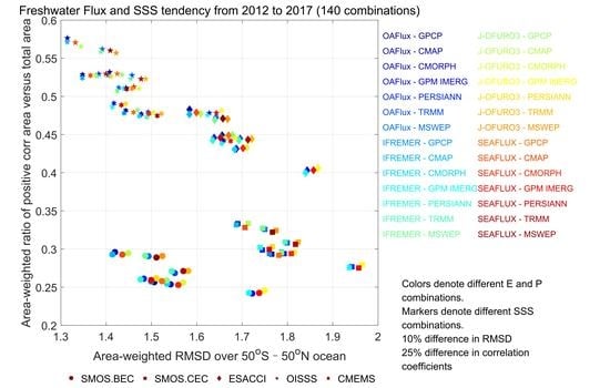
Figure 7 quantifies the correlation between FWF and SSS tendency among 140 sets of combinations between , , and SSS data from 2012 to 2017. To summarize how the correlations vary among different sets, two properties associated with correlation are calculated: the ratio of the spatial coverage of the significantly positive correlation (p-value < 0.05) versus the size of the global ocean and the area-weighted correlation coefficients (along with p-values) from each grid point averaged over the global ocean. The former property indicates the size of the area over the global ocean that the rain gauge-SSS framework might be apt. The latter property is a statistical quantity that is calculated between the FWF and SSS tendency at each grid point and then correlation coefficients are area-weighted averaged over the global ocean. They denote the overall agreement between the FWF and SSS tendency over the global ocean. Values near 0 or negative indicate that the framework for the SSS-rain gauge is not apt for a large portion of the ocean gyres, and values near 1 indicate that the SSS-rain gauge framework is robust.
The two properties mainly vary due to spread in SSS products instead of or (Figure 7). The ratio of the positive correlation area versus total area between 28 sets of FWF and SSS tendencies is 0.27 for SMOS BEC, while those of SMOS CEC, ESACCI, OISSS and CMEMS are 0.3, 0.45, 0.53, and 0.49, respectively. The minimum ratio of size occurs in sets of OAFlux-GPM IMERG-SMOS BEC, with a value of 0.241. In other words, a positive and significant correlation between FWF and SSS tendency for those two sets only occurs over 24.1% of the global ocean between 50°S and 50°N. The maximum size ratio occurs in the set of OAFlux-CMAP-OISSS, with the occurrence of a significant positive correlation over 58% the global oceans. In summary, 24.1~58% of the area over the global ocean shows a significantly positive correlation between the FWF and SSS tendency derived from satellite products, which indicates that the rain gauge-SSS assumption based on satellites is not valid for at least 40% of the global ocean.
The correlation coefficients of FWF and SSS tendency from 2012 to 2017 averaged over the global ocean are small, ranging from 0.11 (OAFlux-GPM IMERG-SMOS BEC) to 0.26 (OAFlux-CMAP-OISSS). Furthermore, p-values for correlation between FWF and SSS tendency over the global ocean from 2012 to 2017 are larger than 0.05 for 140 combinations of , and SSS products (Figure 7b,d,f,h,j). This further confirms the difficulty in treating SSS as a rain gauge over most of the global ocean based on satellite-based SSS and FWF products. The spread in correlation coefficients between SSS tendency and FWF among 140 combinations is 0.05, which denotes a 25% discrepancy. Such a large difference in correlation coefficients among datasets might be attributed to uncertainty associated with different data sources or retrieval methods. A discussion of the possible causes is included in Section 4.
To further explore the linear relationship between FWF and SSS tendency, the two variables are decomposed into two components as a function of time at seasonal and nonseasonal scales (Figure 8). Correlation coefficients between five sets of SSS tendencies and 28 sets of FWFs are calculated at different time scales at each grid point. The ratio of the size of the positive correlation area to the size of the global ocean is compared at different time scales. The same has been compared for correlation coefficients in area-weighted values over the 50°S–50°N ocean. The SSS tendency and FWF on a seasonal time scale are calculated by averaging each month over different years from 2012 to 2017 (total number of freedoms is 10), and nonseasonal anomalies are calculated by subtracting the monthly values from the climatological seasonal values in each month (total number of freedoms is 58).
For ESACCI, OISSS and CMEMS, the sizes of significantly positive correlation coefficient regions on seasonal time scales are 30~40% larger than those on nonseasonal time scales (Figure 8a). For SMOS BEC and CEC, the sizes of significantly positive correlation coefficient regions on the seasonal time scale show nearly the same spatial coverage (or slightly larger for SMOS CEC) as those based on the nonseasonal time scale. The minimum in spatial coverage of both seasonal and nonseasonal positive correlation between FWF and SSS tendency occurs in SMOS BEC among five SSS products, while the maximum in spatial coverage on seasonal correlation occurs in CMEMS, and maximum in those on nonseasonal time scales occurs in OISSS. For the five SSS products, the area-weighted mean correlation coefficients between SSS tendency and FWF over the 50°S–50°N ocean show larger values on seasonal time scales than on nonseasonal time scales (all p-values for seasonal or non-seasonal correlation are larger than 0.05, indicating that correlations are not significant, Figure 8b). The CMEMS shows the largest correlation coefficients on the seasonal time scale, and OISSS shows the largest correlation coefficients on the nonseasonal time scale. The minimum correlation coefficients between SSS tendency and FWF on seasonal and nonseasonal time scales occur in SMOS BEC. The ratio of correlation coefficients on seasonal and nonseasonal time scales is 2~3 for all 140 sets of , and SSS. Based on the results above, the seasonal cycle plays the dominant role in the correlation between FWF and SSS tendency among different time scales.
To examine how the FWF-SSS tendency relation varies on regional scales among products, we show maps of the “best” case (OAFlux-CMAP-OISSS) and the “worst” case (OAFlux-IMERG GPM-SMOS BEC) based on the area-weighted mean correlation coefficients (only sites with p-values < 0.05 and positive correlation coefficients are shown in Figure 9) derived from 2012 to 2017. The correlation coefficients from the best case show a similar spatial pattern to those based on the ensemble median, with the largest values located in the subtropical gyres but insignificant or negative values over the tropical oceans. For the worst case, either the size of positive and significant correlation coefficients or the magnitude of the correlation coefficients is significantly reduced compared to the best case. The maximum correlations from the worst cases mainly occur over the eastern and central subtropical South Pacific Ocean, the eastern North Pacific Ocean, the central South Atlantic Ocean, and the central tropical Indian Ocean. In both the best and worst cases, the magnitude of the correlation coefficients between the FWF and SSS tendency is larger on seasonal time scales than on nonseasonal time scales. This suggests that seasonal SSS can be treated as a rain gauge over some portion (shading in colors in Figure 9c,d) of the ocean, while SSS and FWF on nonseasonal time scales lack such capability.
Figure 10 compares the RMSD between SSS tendency and FWF among 140 sets of products. Similar to the results based on STDs (Figure 5) and correlation (Figure 7), spread in SSS products (STD of RMSD is 0.15 g/kg/year averaged over 28 EMP combinations) makes the largest contribution to the spread in RMSD between SSS tendency and FWF among 140 sets. The spread in RMSD among products is also large, with a magnitude of 0.09 g/kg/year averaged over 20 combinations between the and SSS products. For example, in Figure 10a, a set of SMOS BEC-OAFlux-CMAP is 1.42 g/kg/year, and a set of SMOS BEC-OAFlux-GMP IMERG is 1.72 g/kg/year. The difference between them is 0.3 g/kg/year due to the different P products used. The spread in contributes the least to the spread in RMSD between SSS tendency and FWF among 140 sets of combinations, which indicates a strong consistency among products. The minimum RMSD between FWF and SSS tendency occurs in sets of OAFlux-CMAP-OISSS, with values of 1.314 g/kg/year. The maximum RMSD between FWF and SSS tendency appears in sets of JOFURO-GPM IMERG-SMOS CEC, with values of 1.97 g/kg/year. The mean RMSD averaged among 140 sets of combinations is 1.59 g/kg/year and the spread in RMSD is 0.16 g/kg/year. This result suggests that a 10% difference in RMSD between the SSS tendency and FWF is caused by the different combinations of sets of “--SSS” products.
Figure 11 examines the difference in RMSD between SSS tendency and FWF on seasonal and nonseasonal time scales among 140 sets of data from 2012 to 2017. The RMSD on the seasonal time scale is generally smaller than that on the nonseasonal time scale, except for three sets of OISSS data with FWF that show the same magnitude of RMSD on both seasonal and nonseasonal time scales. The minimum RMSD on nonseasonal time scales occurs in OISSS, with values of approximately 0.95 g/kg/year, while the minimum in seasonal RMSD occurs in CMEMS, with values of 0.9 g/kg/year. The maximum RMSD on seasonal and nonseasonal time scales occurs in SMOS CEC, with values of 1.22 g/kg/year for the former and 1.58 g/kg/year for the latter.
4. Discussion
We present an intercomparison of satellite-based four products, seven products and five SSS products over the 50°S–50°N ocean from 2012 to 2017 and assess the relation between SSS and FWF using 140 combinations of , and SSS products. For each variable, the variability from individual products is compared with the ensemble median values (Figure 2 and Figure 3e). Maximum deviations from the ensemble median, measured by RMSD, occur in J-OFURO3 for (Figure 2), GPM IMERG for (Figure 2), and SMOS CEC for SSS (Figure 3e). Datasets that show the largest difference from the ensemble median do not imply a weak representation of the “true value”. To examine the capability of an air–sea freshwater exchange property in representing the true value, this property should be examined from a property-conserved perspective. For example, examining in water budget (if the net transport of water vapor from ocean to land is known [95]) or oceanic freshwater budget [100] by using different sets of products could offer a way to rank the results of intercomparison.
The area-weighted variability of EMP (Figure 2c,d) over the global ocean from monthly data from 2012 to 2017 is 2.4 mm/day, which is stronger than (0.85 mm/day) and (2.17 mm/day), respectively. It also infers that the deviation among data is dominated by differences in , which agrees with results from Gutenstein et al. [95], who use a different set of and and period (1993–2017) from this analysis. SMOS CEC shows the largest variability (0.22 g/kg in Figure 3e) among the five satellite-based SSS products, and SMOS BEC shows the smallest variability (0.18 g/kg). Liu and Wei [92] have compared 10 SSS estimates from 2011 to 2018 using a combination of in situ and satellite-based data. They also found that SMOS CEC (called LOCEAN in their study, which is an early version of SMOS CEC v7) shows the largest variability among the 10 SSS datasets during 2011–2018. Thus, SMOS CEC contributes the most to the spread/uncertainty not only in satellite-based SSS but also for in situ and satellite combined sets of products.
The SSS tendency derived from the 2012–2017 mean is 1~2 magnitude smaller than that of FWF (Figure 4a,b), consistent with results from Ponte and Vinogradova [14], in which they showed that the salinity tendency at 5 m based on a closed salinity budget model is two orders of magnitude smaller than that of the FWF over 1993–2010. The high consistency between the two results suggests the possibility of using satellite SSS as an independent reference for validating the bulk-SSS budget. To assess the relation between SSS and FWF in satellite-based products, we calculate their STDs, correlations and RMSD. These variables offer the temporal variations or relation over 50°S–50°N from 2012 to 2017 among different products. For STDs, there is at least a 15% difference in SSS tendency among the five SSS datasets, and a 10% for FWF among the 28 combinations between the and products. For the area-weighted mean correlation coefficient over the global ocean from 2012 to 2017, there is 25% difference between SSS tendency and FWF if different combinations of --SSS products are chosen. There is a 10% difference in RMSD between the SSS tendency and FWF, which is caused by the different combinations of sets of --SSS products. These differences among products prevent the use of a single combination of --SSS as a reference for evaluating SSS budgets.
It should be noted that the satellite-based over the ocean is estimated from principles of infrared and microwave retrievals [22]. cannot be directly observed over the ocean and is often estimated from other variables based on bulk formulas [91,101]. SSS products based on satellites generally retrieve data from L-band brightness temperatures [102]. Thus, the derivations for satellite-based , and SSS are all indirect. The results are inevitably accompanied by a large amount of uncertainty. Different retrieval algorithms or data sources might be responsible for the large uncertainty in , , and SSS products or EMP - SSS relations among products. Further analysis is needed to identify the main cause. For example, to examine whether the retrieving methods are the main causes for the difference, one should use the same sources of data and apply different retrieving methods.
5. Summary
This study aims to quantify the uncertainty in satellite-based SSS, , and and examine the roles of such uncertainty in the relation between EMP and SSS based on 140 sets of combinations between , and SSS. Statistical properties are calculated over the 50°S–50°N ocean from 2012 to 2017. Maximum variability in satellite-based SSS occurs in SMOS CEC, and minimum variability occurs in SMOS BEC. For FWF, the largest variability occurs in J-OFURO3-GPM IMERG, and the minimum occurs in IFREMER-CMAP. The minimum (maximum) RMSD between FWF and SSS tendency occurs in sets of OAFlux-CMAP-OISSS (JOFURO-GPM IMERG-SMOS CEC), with values of 1.31 g/kg/year (1.97 g/kg/year). The area-weighted correlation coefficient between SSS tendency and FWF from 2012 to 2017 is generally small among 140 sets of combinations of --SSS, with values from 0.11 (OAFlux-CMAP-OISSS) to 0.26 (OAFlux-GPM IMERG-SMOS BEC). p-values for correlation among 140 sets of combinations are larger than 0.05. Further analysis reveals that 24.1~58% (variations based on different sets of products) of the area over the global ocean shows significantly positive correlation coefficients between FWF and SSS tendency derived from satellite products, which indicates that the rain gauge-SSS could be valid there. Properties calculated from 2012 to 2017 over the 50°S–50°N ocean between FWF and SSS tendency show an uncertainty of 25% in correlation coefficients and an uncertainty of 10% in RMSD. As large discrepancies in the FWF-SSS relationship exist among sets of --SSS, the results of this study warn against the use of any combination of , and SSS from a single product for salinity budget analysis or oceanic hydrological cycle-related budget analysis. Furthermore, this study could serve as a benchmark for constraining satellite-based , and SSS uncertainty in the model in which FWF and SSS can be derived based on each other alone [103].
For STDs, correlation coefficients and RMSD, we also found out that the spread in those properties between FWF and SSS tendency is mainly attributed to the spread in SSS products instead of or . The uncertainty in the STDs of the SSS tendency and FWF are 15% and 10%, respectively. This warrants an urgent need for improving the consistency in satellite-based SSS products. Further analysis shows that the FWF and SSS tendencies at the seasonal time scale show larger correlation coefficients and lower RMSDs than those at the nonseasonal time scale in most sets of 140 combinations. Statistically, satellite-based FWF and SSS tendencies have better similarities (from correlation and RMSD perspectives) in temporal variability over 50°S–50°N on seasonal time scales than at other time scales. Thus, perhaps on a seasonal time scale, over limited regions (Figure 9), SSS can be used as a rain gauge, but it is not possible anywhere over the global ocean on any time scale.
We emphasize that some major contributions to SSS tendency (such as advection [12,13]) are unknown, and whether the worst or the best cases (Figure 9) are closer to the salinity budget conservation is not identifiable based on our results. As ocean dynamics [12] and near-surface salinity stratification [20] could account for the difference between the FWF and SSS tendencies observed in this study, global-scale and long-term in situ observations with the capability of detecting skin salinity are still needed to validate the results based on satellites. However, the outcome of this study offers a possible range of variations which we could use as a reference for constraining model stimulations.
Author Contributions
Conceptualization, H.L. and Z.W.; methodology, H.L.; software, H.L.; validation, H.L., and X.N.; formal analysis, H.L.; investigation, H.L.; writing—original draft preparation, H.L.; writing—review and editing, H.L., Z.W. and X.N. All authors have read and agreed to the published version of the manuscript.
Funding
This research was funded by the National Natural Science Foundation of China (42006005, 41821004, 41806040).
Institutional Review Board Statement
Not applicable.
Informed Consent Statement
Not applicable.
Data Availability Statement
All data are freely available at following websites. Some of the datasets are required to be registered before accessing. GPCP version 3.1 is accessible at https://disc.gsfc.nasa.gov/datasets/GPCPMON_3.1/summary?keywords=GPCPMON_3.1; CMAP at https://psl.noaa.gov/data/gridded/data.cmap.html#detail; TRMM 3B42 at https://disc.gsfc.nasa.gov/datasets/TRMM_3B42_7/summary?keywords=TRMM%203B42; GPM IMERG at https://doi.org/10.5067/GPM/IMERG/3B-MONTH/06; PERSIANN CDR at https://chrsdata.eng.uci.edu/; CMORPH at https://doi.org/10.5065/0EFN-KZ90; MSWEP at http://www.gloh2o.org/mswep/; OAFlux at https://oaflux.whoi.edu/; IFREMER v4.1 at https://wwz.ifremer.fr/oceanheatflux/Data; SEAFLUX3 at http://dx.doi.org/10.5067/SEAFLUX/DATA101; J-OFURO3 at https://j-ofuro.isee.nagoya-u.ac.jp/en/; SMOS BEC at http://bec.icm.csic.es/ocean-global-sss/; SMOS CEC at https://www.seanoe.org/data/00417/52804/; ESACCI at https://climate.esa.int/en/odp/#/project/sea-surface-salinity; OISSS at https://podaac.jpl.nasa.gov/dataset/OISSS_L4_multimission_7day_v1;CMEMS at https://resources.marine.copernicus.eu/product-detail/MULTIOBS_GLO_PHY_S_SURFACE_MYNRT_015_013/; IFREMER MLD at http://www.ifremer.fr/cerweb/deboyer/mld/Surface_Mixed_Layer_Depth.php. All data were accessed 20 April 2022.
Acknowledgments
This research thanks the National Natural Science Foundation of China (42006005, 41821004, 41806040) for their financial support.
Conflicts of Interest
The authors declare no conflict of interest.
References
- Bingham, F.M.; Foltz, G.; McPhaden, M. Characteristics of the seasonal cycle of surface layer salinity in the global ocean. Ocean Sci. 2012, 8, 915–929. [Google Scholar] [CrossRef] [Green Version]
- Elliott, G.W. Precipitation signatures in sea-surface-layer conditions during BOMEX. J. Phys. Oceanogr. 1974, 4, 498–501. [Google Scholar] [CrossRef] [Green Version]
- Durack, P.J.; Wijffels, S.E. Fifty-year trends in global ocean salinities and their relationship to broad-scale warming. J. Clim. 2010, 23, 4342–4362. [Google Scholar] [CrossRef]
- Helm, K.P.; Bindoff, N.L.; Church, J.A. Changes in the global hydrological-cycle inferred from ocean salinity. Geophys. Res. Lett. 2010, 37, L18701. [Google Scholar] [CrossRef]
- Lago, V.; Wijffels, S.E.; Durack, P.J.; Church, J.A.; Bindoff, N.L.; Marsland, S.J. Simulating the role of surface forcing on observed multidecadal upper ocean salinity changes. J. Clim. 2015, 29, 5575–5588. [Google Scholar] [CrossRef]
- Baumgartner, A.; Reichel, E. The World Water Balance: Mean Annual Global, Continental and Maritime Precipitation and Run-Off; Elsevier: Amsterdam, The Netherlands, 1975. [Google Scholar]
- Durack, P.J.; Wijffels, S.E.; Matear, R.J. Ocean salinities reveal strong global water cycle intensification during 1950 to 2000. Science 2012, 336, 455–458. [Google Scholar] [CrossRef] [PubMed] [Green Version]
- Dorigo, W.; Dietrich, S.; Aires, F.; Brocca, L.; Carter, S.; Cretaux, J.-F.; Dunkerley, D.; Enomoto, H.; Forsberg, R.; Güntner, A.; et al. Closing the Water Cycle from Observations across Scales: Where Do We Stand? Bull. Am. Meteorol. Soc. 2021, 102, E1897–E1935. [Google Scholar] [CrossRef]
- Hosoda, S.; Suga, T.; Shikama, N.; Mizuno, K. Global surface layer salinity change detected by Argo and its implication for hydrological cycle intensification. J. Oceanogr. 2009, 65, 579–586. [Google Scholar] [CrossRef]
- Terray, L.; Corre, L.; Cravatte, S.; Delcroix, T.; Reverdin, G.; Ribes, A. Near-surface salinity as nature's rain gauge to detect human influence on the tropical water cycle. J. Clim. 2012, 25, 958–977. [Google Scholar] [CrossRef] [Green Version]
- Yu, L. A global relationship between the ocean water cycle and near-surface salinity. J. Geophys. Res. Ocean. 2011, 116, C10025. [Google Scholar] [CrossRef]
- Vinogradova, N.T.; Ponte, R.M. Clarifying the link between surface salinity and freshwater fluxes on monthly to interannual time scales. J. Geophys. Res. Ocean 2013, 118, 3190–3201. [Google Scholar] [CrossRef]
- Vinogradova, N.T.; Ponte, R.M. In Search of Fingerprints of the Recent Intensification of the Ocean Water Cycle. J. Clim. 2017, 30, 5513–5528. [Google Scholar] [CrossRef]
- Ponte, R.; Vinogradova, N. An assessment of basic processes controlling mean surface salinity over the global ocean. Geophys. Res. Lett. 2016, 43, 7052–7058. [Google Scholar] [CrossRef] [Green Version]
- Yu, L.; Jin, X.; Josey, S.A.; Lee, T.; Kumar, A.; Wen, C.; Xue, Y. The Global Ocean Water Cycle in Atmospheric Reanalysis, Satellite, and Ocean Salinity. J. Clim. 2017, 30, 3829–3852. [Google Scholar] [CrossRef]
- Grodsky, S.A.; Carton, J.A. Delayed and Quasi-Synchronous Response of Tropical Atlantic Surface Salinity to Rainfall. J. Geophys. Res. Ocean. 2018, 123, 5971–5985. [Google Scholar] [CrossRef]
- Tzortzi, E. Sea Surface Salinity in the Atlantic Ocean from the SMOS Mission and Its Relation to Freshwater Fluxes. Ph.D. Thesis, University of Southampton, Southampton, UK, 2015. [Google Scholar]
- Yueh, S.H.; West, R.; Wilson, W.J.; Li, F.K.; Njoku, E.G.; Rahmat-Samii, Y. Error sources and feasibility for microwave remote sensing of ocean surface salinity. IEEE Trans. Geosci. Remote Sens. 2001, 39, 1049–1060. [Google Scholar] [CrossRef] [Green Version]
- Henocq, C.; Boutin, J.; Reverdin, G.; Petitcolin, F.; Arnault, S.; Lattes, P. Vertical Variability of Near-Surface Salinity in the Tropics: Consequences for L-Band Radiometer Calibration and Validation. J. Atmos. Ocean. Technol. 2010, 27, 192–209. [Google Scholar] [CrossRef]
- Boutin, J.; Chao, Y.; Asher, W.E.; Delcroix, T.; Drucker, R.; Drushka, K.; Kolodziejczyk, N.; Lee, T.; Reul, N.; Reverdin, G. Satellite and in situ salinity: Understanding near-surface stratification and subfootprint variability. Bull. Am. Meteorol. Soc. 2016, 97, 1391–1407. [Google Scholar] [CrossRef] [Green Version]
- Stammer, D.; Martins, M.S.; Köhler, J.; Köhl, A. How well do we know ocean salinity and its changes? Prog. Oceanogr 2021, 190, 102478. [Google Scholar] [CrossRef]
- Kidd, C.; Huffman, G. Global precipitation measurement. Meteorol. Appl. 2011, 18, 334–353. [Google Scholar] [CrossRef]
- Huffman, G.J.; Behrangi, A.; Bolvin, D.T.; Nelkin, E.J. (Eds.) GPCP Version 3.1 Satellite-Gauge (SG) Combined Precipitation Data Set; NASA GES DISC: Greenbelt, MD, USA, 2020. [Google Scholar] [CrossRef]
- Adler, R.F.; Huffman, G.J.; Keehn, P.R. Global tropical rain estimates from microwave-adjusted geosynchronous IR data. Remote Sens. Rev. 1994, 11, 125–152. [Google Scholar] [CrossRef]
- Susskind, J.; Piraino, P.; Rokke, L.; Iredell, L.; Mehta, A. Characteristics of the TOVS Pathfinder Path A dataset. Bull. Am. Meteorol. Soc. 1997, 78, 1449–1472. [Google Scholar] [CrossRef]
- Huffman, G.J.; Adler, R.F.; Bolvin, D.T.; Hsu, K.; Kidd, C.; Nelkin, E.J.; Tan, J.; Xie, P. Algorithm Theoretical Basis Document (ATBD) for Global Precipitation Climatology Project Version 3.0 Precipitation Data; MEaSUREs project: Greenbelt, MD, USA, 2019. [Google Scholar]
- Xie, P.; Arkin, P.A. Global Precipitation: A 17-Year Monthly Analysis Based on Gauge Observations, Satellite Estimates, and Numerical Model Outputs. Bull. Am. Meteorol. Soc. 1997, 78, 2539–2558. [Google Scholar] [CrossRef]
- Xie, P.; Joyce, R.; Wu, S.; Yoo, S.; Yarosh, Y.; Sun, F.; Lin, R. NOAA Climate Data Record (CDR) of CPC Morphing Technique (CMORPH) High Resolution Global Precipitation Estimates, Version 1; RDA/UCAR: Research Data Archive at the National Center for Atmospheric Research; Computational and Information Systems Laboratory, National Centers for Environmental Information, NESDIS, NOAA: Greenbelt, MD, USA, 2020. [Google Scholar] [CrossRef]
- Huffman, G.J.; Stocker, E.F.; Bolvin, D.T.; Nelkin, E.J.; Tan, J. GPM IMERG Final Precipitation L3 1 Month 0.1 Degree x 0.1 Degree V06; Goddard Earth Sciences Data and Information Services Center: Greenbelt, MD, USA, 2019. [Google Scholar] [CrossRef]
- Ashouri, H.; Hsu, K.-L.; Sorooshian, S.; Braithwaite, D.K.; Knapp, K.R.; Cecil, L.D.; Nelson, B.R.; Prat, O.P. PERSIANN-CDR: Daily precipitation climate data record from multisatellite observations for hydrological and climate studies. Bull. Am. Meteorol. Soc. 2015, 96, 69–83. [Google Scholar] [CrossRef] [Green Version]
- Huffman, G.J.; Bolvin, D.T.; Nelkin, E.J.; Wolff, D.B.; Adler, R.F.; Gu, G.; Hong, Y.; Bowman, K.P.; Stocker, E.F. The TRMM Multisatellite Precipitation Analysis (TMPA): Quasi-Global, Multiyear, Combined-Sensor Precipitation Estimates at Fine Scales. J. Hydrometeorol. 2007, 8, 38–55. [Google Scholar] [CrossRef]
- Beck, H.E.; van Dijk, A.I.J.M.; Levizzani, V.; Schellekens, J.; Miralles, D.G.; Martens, B.; de Roo, A. MSWEP: 3-hourly 0.25° global gridded precipitation (1979–2015) by merging gauge, satellite, and reanalysis data. Hydrol. Earth Syst. Sci. 2017, 21, 589–615. [Google Scholar] [CrossRef] [Green Version]
- Beck, H.E.; Wood, E.F.; Pan, M.; Fisher, C.K.; Miralles, D.G.; Van Dijk, A.I.; McVicar, T.R.; Adler, R.F. MSWEP V2 global 3-hourly 0.1 precipitation: Methodology and quantitative assessment. Bull. Am. Meteorol. Soc. 2019, 100, 473–500. [Google Scholar] [CrossRef] [Green Version]
- Yu, L.; Weller, R.A. Objectively Analyzed Air–Sea Heat Fluxes for the Global Ice-Free Oceans (1981–2005). Bull. Am. Meteorol. Soc. 2007, 88, 527–540. [Google Scholar] [CrossRef] [Green Version]
- Bentamy, A.; Grodsky, S.A.; Katsaros, K.; Mestas-Nuñez, A.M.; Blanke, B.; Desbiolles, F. Improvement in air–sea flux estimates derived from satellite observations. Int. J. Remote Sens. 2013, 34, 5243–5261. [Google Scholar] [CrossRef] [Green Version]
- Tomita, H.; Hihara, T.; Kako, S.I.; Kubota, M.; Kutsuwada, K. An introduction to J-OFURO3, a third-generation Japanese ocean flux data set using remote-sensing observations. J. Oceanogr. 2019, 75, 171–194. [Google Scholar] [CrossRef] [Green Version]
- Roberts, B.J.; Clayson, C.A.; Robertson, F.R. SeaFlux Data Products; NASA Global Hydrology Resource Center DAAC: Huntsville, AL, USA, 2020. [Google Scholar]
- Olmedo, E.; González-Haro, C.; Hoareau, N.; Umbert, M.; González-Gambau, V.; Martínez, J.; Gabarró, C.; Turiel, A. Nine years of SMOS sea surface salinity global maps at the Barcelona Expert Center. Earth Syst. Sci. Data 2021, 13, 857–888. [Google Scholar] [CrossRef]
- Boutin, J.; Vergely, J.-L.; Khvorostyanov, D. SMOS SSS L3 Maps Generated by CATDS CEC LOCEAN. Debias V7.0. SEANOE; SEANOE: Plouzané, France, 2022. [Google Scholar] [CrossRef]
- Boutin, J.; Reul, N.; Catany, R.; Koehler, J.; Martin, A.; Rouffi, F.; Arias, M.; Chakroun, M.; Corato, G.; Estella-Perez, V.; et al. ESA Sea Surface Salinity Climate Change Initiative (Sea_Surface_Salinity_cci): Weekly and Monthly Sea Surface Salinity Prod-ucts, v2. 31, for 2010 to 2019. 07 September 2020 ed.; NERC EDS Centre for Environmental Data Analysis: Gwynedd, UK, 2020. [Google Scholar] [CrossRef]
- Melnichenko, O. Multi-Mission Optimally Interpolated Sea Surface Salinity 7-Day Global Dataset V1; NASA Physical Oceanography DAAC: PO.DAAC: Pasadena, CA, USA, 2021. [Google Scholar] [CrossRef]
- Droghei, R.; Nardelli, B.B.; Santoleri, R. Combining in situ and satellite observations to retrieve salinity and density at the ocean surface. J. Atmos. Ocean. Technol. 2016, 33, 1211–1223. [Google Scholar] [CrossRef]
- Kalnay, E.; Kanamitsu, M.; Kistler, R.; Collins, W.; Deaven, D.; Gandin, L.; Iredell, M.; Saha, S.; White, G.; Woollen, J.; et al. The NCEP/NCAR 40-Year Reanalysis Project. Bull. Am. Meteorol. Soc. 1996, 77, 437–472. [Google Scholar] [CrossRef] [Green Version]
- Olson, W.S.; Masunaga, H. GMP.Combined Radar-Radiometer Algorithm Team. In GPM Combined Radar-Radiometer Precipitation Algorithm Theoretical Basis Document (Version 4); NASA: Washington, DC, USA, 2016. [Google Scholar]
- Knapp, K.R. Scientific data stewardship of International Satellite Cloud Climatology Project B1 global geostationary observations. J. Appl. Remote Sens. 2008, 2, 023548. [Google Scholar] [CrossRef]
- Adler, R.F.; Sapiano, M.R.; Huffman, G.J.; Wang, J.-J.; Gu, G.; Bolvin, D.; Chiu, L.; Schneider, U.; Becker, A.; Nelkin, E. The Global Precipitation Climatology Project (GPCP) monthly analysis (new version 2.3) and a review of 2017 global precipitation. Atmosphere 2018, 9, 138. [Google Scholar] [CrossRef] [Green Version]
- Dee, D.P.; Uppala, S.; Simmons, A.; Berrisford, P.; Poli, P.; Kobayashi, S.; Andrae, U.; Balmaseda, M.; Balsamo, G.; Bauer, P. The ERA-Interim reanalysis: Configuration and performance of the data assimilation system. Q. J. R. Meteorol. Soc. 2011, 137, 553–597. [Google Scholar] [CrossRef]
- Schneider, U.; Becker, A.; Finger, P.; Meyer-Christoffer, A.; Ziese, M.; Rudolf, B. GPCC’s new land surface precipitation climatology based on quality-controlled in situ data and its role in quantifying the global water cycle. Theor. Appl. Climatol. 2014, 115, 15–40. [Google Scholar] [CrossRef] [Green Version]
- Schneider, U.; Finger, P.; Meyer-Christoffer, A.; Rustemeier, E.; Ziese, M.; Becker, A. Evaluating the Hydrological Cycle over Land Using the Newly-Corrected Precipitation Climatology from the Global Precipitation Climatology Centre (GPCC). Atmosphere 2017, 8, 52. [Google Scholar] [CrossRef] [Green Version]
- Knapp, K.R.; Ansari, S.; Bain, C.L.; Bourassa, M.A.; Dickinson, M.J.; Funk, C.; Helms, C.N.; Hennon, C.C.; Holmes, C.D.; Huffman, G.J.; et al. Globally Gridded Satellite Observations for Climate Studies. Bull. Am. Meteorol. Soc. 2011, 92, 893–907. [Google Scholar] [CrossRef]
- Ushio, T.; Sasashige, K.; Kubota, T.; Shige, S.; Okamoto, K.; Aonashi, K.; Inoue, T.; Takahashi, N.; Iguchi, T.; Kachi, M.; et al. A Kalman Filter Approach to the Global Satellite Mapping of Precipitation (GSMaP) from Combined Passive Microwave and Infrared Radiometric Data. J. Meteorol. Soc. Japan. Ser. II 2009, 87A, 137–151. [Google Scholar] [CrossRef] [Green Version]
- Kobayashi, S.; Ota, Y.; Harada, Y.; Ebita, A.; Moriya, M.; Onoda, H.; Onogi, K.; Kamahori, H.; Kobayashi, C.; Endo, H.; et al. The JRA-55 Reanalysis: General Specifications and Basic Characteristics. J. Meteorol. Soc. Japan. Ser. II 2015, 93, 5–48. [Google Scholar] [CrossRef] [Green Version]
- Fick, S.E.; Hijmans, R.J. WorldClim 2: New 1-km spatial resolution climate surfaces for global land areas. Int. J. Climatol. 2017, 37, 4302–4315. [Google Scholar] [CrossRef]
- Singh, R.; Joshi, P.; Kishtawal, C. A new technique for estimation of surface latent heat fluxes using satellite-based observations. Mon. Weather Rev. 2005, 133, 2692–2710. [Google Scholar] [CrossRef]
- Kanamitsu, M.; Ebisuzaki, W.; Woollen, J.; Yang, S.-K.; Hnilo, J.J.; Fiorino, M.; Potter, G.L. NCEP–DOE AMIP-II Reanalysis (R-2). Bull. Am. Meteorol. Soc. 2002, 83, 1631–1644. [Google Scholar] [CrossRef]
- Reynolds, R.W.; Smith, T.M.; Liu, C.; Chelton, D.B.; Casey, K.S.; Schlax, M.G. Daily High-Resolution-Blended Analyses for Sea Surface Temperature. J. Clim. 2007, 20, 5473–5496. [Google Scholar] [CrossRef]
- Fairall, C.W.; Bradley, E.F.; Hare, J.E.; Grachev, A.A.; Edson, J.B. Bulk Parameterization of Air–Sea Fluxes: Updates and Verification for the COARE Algorithm. J. Clim. 2003, 16, 571–591. [Google Scholar] [CrossRef]
- Kummerow, D.C.; Berg, W.K.; Sapiano, M.R.; Program, N.C. NOAA Climate Data Record (CDR) of SSM/I and SSMIS Microwave Brightness Temperatures, CSU Version 1; National Centers for Environmental Information, NESDIS, NOAA: Greenbelt, MD, USA, 2013. [Google Scholar] [CrossRef]
- Freeman, E.; Woodruff, S.D.; Worley, S.J.; Lubker, S.J.; Kent, E.C.; Angel, W.E.; Berry, D.I.; Brohan, P.; Eastman, R.; Gates, L.; et al. ICOADS Release 3.0: A major update to the historical marine climate record. Int. J. Climatol. 2017, 37, 2211–2232. [Google Scholar] [CrossRef] [Green Version]
- Berrisford, P.; Dee, D.P.; Poli, P.; Brugge, R.; Fielding, M.; Fuentes, M.; Kållberg, P.W.; Kobayashi, S.; Uppala, S.; Simmons, A. The ERA-Interim archive Version 2.0; ECMWF: Shinfield, UK, 2011; Volume 23. [Google Scholar]
- Bentamy, A.; Grodsky, S.A.; Elyouncha, A.; Chapron, B.; Desbiolles, F. Homogenization of scatterometer wind retrievals. Int. J. Climatol. 2017, 37, 870–889. [Google Scholar] [CrossRef] [Green Version]
- Tomita, H.; Hihara, T.; Kubota, M. Improved Satellite Estimation of Near-Surface Humidity Using Vertical Water Vapor Profile Information. Geophys. Res. Lett. 2018, 45, 899–906. [Google Scholar] [CrossRef]
- Wentz, F.J.; Ricciardulli, L.; Gentemann, C.; Meissner, T.; Hilburn, K.A.; Scott, J. Remote Sensing Systems Coriolis WindSat, Environmental Suite on 0.25 deg grid, Version 7.0.1.; Remote Sensing Systems: Santa Rosa, CA, USA, 2013. [Google Scholar]
- Wentz, F.J. A 17-yr climate record of environmental parameters derived from the Tropical Rainfall Measuring Mission (TRMM) Microwave Imager. J. Clim. 2015, 28, 6882–6902. [Google Scholar] [CrossRef]
- Gaiser, P.W.; St Germain, K.M.; Twarog, E.M.; Poe, G.A.; Purdy, W.; Richardson, D.; Grossman, W.; Jones, W.L.; Spencer, D.; Golba, G. The WindSat spaceborne polarimetric microwave radiometer: Sensor description and early orbit performance. IEEE Trans. Geosci. Remote Sens. 2004, 42, 2347–2361. [Google Scholar] [CrossRef]
- Piolle, J.-F.; Bentamy, A. Quickscat scatterometer-Mean wind fileds products-User Manual. Ifremer, Department of Oceanography from Space, Ref.: C2-MUT-W-03-IF, Version 1.0. 2002. Available online: http://apdrc.soest.hawaii.edu/doc/qscat_mwf.pdf (accessed on 20 April 2022).
- Berg, W.; Kroodsma, R.; Kummerow, C.D.; McKague, D.S. Fundamental Climate Data Records of Microwave Brightness Temperatures. Remote Sens. 2018, 10, 1306. [Google Scholar] [CrossRef] [Green Version]
- Roberts, J.B.; Clayson, C.A.; Robertson, F.R. Improving Near-Surface Retrievals of Surface Humidity Over the Global Open Oceans From Passive Microwave Observations. Earth Space Sci. 2019, 6, 1220–1233. [Google Scholar] [CrossRef] [PubMed] [Green Version]
- Roberts, J.B.; Clayson, C.A.; Robertson, F.R.; Jackson, D.L. Predicting near-surface atmospheric variables from Special Sensor Microwave/Imager using neural networks with a first-guess approach. J. Geophys. Res. Atmos. 2010, 115, D19113. [Google Scholar] [CrossRef]
- Gelaro, R.; McCarty, W.; Suárez, M.J.; Todling, R.; Molod, A.; Takacs, L.; Randles, C.A.; Darmenov, A.; Bosilovich, M.G.; Reichle, R.; et al. The Modern-Era Retrospective Analysis for Research and Applications, Version 2 (MERRA-2). J. Clim. 2017, 30, 5419–5454. [Google Scholar] [CrossRef]
- Edson, J.B.; Jampana, V.; Weller, R.A.; Bigorre, S.P.; Plueddemann, A.J.; Fairall, C.W.; Miller, S.D.; Mahrt, L.; Vickers, D.; Hersbach, H. On the Exchange of Momentum over the Open Ocean. J. Phys. Oceanogr. 2013, 43, 1589–1610. [Google Scholar] [CrossRef] [Green Version]
- Droppleman, J.D.; Mennella, R.A.; Evans, D.E. An airborne measurement of the salinity variations of the Mississippi River Outflow. J. Geophys. Res. 1970, 75, 5909–5913. [Google Scholar] [CrossRef]
- Lagerloef, G.; Colomb, F.R.; Le Vine, D.; Wentz, F.; Yueh, S.; Ruf, C.; Lilly, J.; Gunn, J.; Chao, Y.; Decharon, A. The Aquarius/SAC-D mission: Designed to meet the salinity remote-sensing challenge. Oceanography 2008, 21, 68–81. [Google Scholar] [CrossRef] [Green Version]
- Reul, N.; Fournier, S.; Boutin, J.; Hernandez, O.; Maes, C.; Chapron, B.; Alory, G.; Quilfen, Y.; Tenerelli, J.; Morisset, S.; et al. Sea surface salinity observations from space with the SMOS satellite: A new means to monitor the marine branch of the water cycle. Earth’s Hydrol. Cycle 2014, 35, 681–722. [Google Scholar] [CrossRef] [Green Version]
- Meissner, T.; Wentz, F.J. Remote Sensing Systems SMAP Ocean Surface Salinities [Level 2C, Level 3 Running 8-day, Level 3 Monthly], Version 2.0 Validated Release; Systems, R.S., Ed.; Santa Rosa, CA, USA, 2016. [Google Scholar] [CrossRef]
- Olmedo, E.; Martínez, J.; Turiel, A.; Ballabrera-Poy, J.; Portabella, M. Debiased non-Bayesian retrieval: A novel approach to SMOS Sea Surface Salinity. Remote Sens. Environ. 2017, 193, 103–126. [Google Scholar] [CrossRef]
- Zweng, M.M.; Reagan, J.R.; Antonov, J.I.; Locarnini, R.A.; Mishonov, A.V.; Boyer, T.P.; Garcia, H.E.; Baranova, O.K.; Johnson, D.R.; Seidov, D.; et al. World Ocean Atlas 2013, Volume 2: Salinity; Levitus, S., Mishonov, A., Eds.; Technical Ed: NOAA Atlas NESDIS 74; National Oceanographic Data Center: Silver Spring, MD, USA, 2013. [Google Scholar]
- Donlon, C.J.; Martin, M.; Stark, J.; Roberts-Jones, J.; Fiedler, E.; Wimmer, W. The operational sea surface temperature and sea ice analysis (OSTIA) system. Remote Sens. Environ. 2012, 116, 140–158. [Google Scholar] [CrossRef]
- Boutin, J.; Martin, N.; Kolodziejczyk, N.; Reverdin, G. Interannual anomalies of SMOS sea surface salinity. Remote Sens. Environ. 2016, 180, 128–136. [Google Scholar] [CrossRef]
- Boutin, J.; Vergely, J.-L.; Marchand, S.; d’Amico, F.; Hasson, A.; Kolodziejczyk, N.; Reul, N.; Reverdin, G.; Vialard, J. New SMOS Sea Surface Salinity with reduced systematic errors and improved variability. Remote Sens. Environ. 2018, 214, 115–134. [Google Scholar] [CrossRef] [Green Version]
- Kolodziejczyk, N.; Prigent-Mazella, A.; Gaillard, F. ISAS Temperature and Salinity Gridded Fields; SEANOE: Plouzané, France, 2021. [Google Scholar] [CrossRef]
- Kolodziejczyk, N.; Prigent-Mazella, A.; Gaillard, F. ISAS-SSS: In Situ Sea Surface Salinity Gridded Fields; SEANOE: Plouzané, France, 2018. [Google Scholar] [CrossRef]
- Boutin, J.; Reul, N.; Koehler, J.; Martin, A.; Catany, R.; Guimbard, S.; Rouffi, F.; Vergely, J.L.; Arias, M.; Chakroun, M.; et al. Satellite-Based Sea Surface Salinity Designed for Ocean and Climate Studies. J. Geophys. Res. Ocean. 2021, 126, e2021JC017676. [Google Scholar] [CrossRef]
- Roemmich, D.; Gilson, J. The 2004–2008 mean and annual cycle of temperature, salinity, and steric height in the global ocean from the Argo Program. Prog. Oceanogr. 2009, 82, 81–100. [Google Scholar] [CrossRef]
- Good, S.A.; Martin, M.J.; Rayner, N.A. EN4: Quality controlled ocean temperature and salinity profiles and monthly objective analyses with uncertainty estimates. J. Geophys. Res. Ocean. 2013, 118, 6704–6716. [Google Scholar] [CrossRef]
- Nardelli, B.B. A Novel Approach for the High-Resolution Interpolation of In Situ Sea Surface Salinity. J. Atmos. Ocean. Technol. 2012, 29, 867–879. [Google Scholar] [CrossRef]
- CATDS. CATDS-PDC L3OS 2Q—Debiased Daily Valid Ocean Salinity Values Product from SMOS Satellite; CATDS, Ed.; CNES, IFREMER, LOCEAN, ACRI: Brest, France, 2022. [Google Scholar]
- Boutin, J.; Vergely, J.-L.; Khvorostyanov, D. SMOS SSS L3 Maps Generated by CATDS CEC LOCEAN. Debias V3. 0; SEANOE: Plouzané, France, 2018. [Google Scholar]
- de Boyer Montégut, C.; Madec, G.; Fischer, A.S.; Lazar, A.; Iudicone, D. Mixed layer depth over the global ocean: An examination of profile data and a profile-based climatology. J. Geophys. Res. Ocean. 2004, 109, C12003. [Google Scholar] [CrossRef]
- Henderson-Sellers, B. A new formula for latent heat of vaporization of water as a function of temperature. Q. J. R. Meteorol. Soc. 1984, 110, 1186–1190. [Google Scholar] [CrossRef]
- Fairall, C.W.; Bradley, E.F.; Rogers, D.P.; Edson, J.B.; Young, G.S. Bulk parameterization of air-sea fluxes for Tropical Ocean-Global Atmosphere Coupled-Ocean Atmosphere Response Experiment. J. Geophys. Res. Ocean. 1996, 101, 3747–3764. [Google Scholar] [CrossRef]
- Liu, H.; Wei, Z. Intercomparison of Global Sea Surface Salinity from Multiple Datasets over 2011–2018. Remote Sens. 2021, 13, 811. [Google Scholar] [CrossRef]
- Taylor, K.E. Summarizing multiple aspects of model performance in a single diagram. J. Geophys. Res. Atmos. 2001, 106, 7183–7192. [Google Scholar] [CrossRef]
- McDougall, T.J.; Barker, P.M. Getting started with TEOS-10 and the Gibbs Seawater (GSW), Oceanographic Toolbox. SCOR/IAPSO WG 2011, 127, 1–28. [Google Scholar]
- Gutenstein, M.; Fennig, K.; Schröder, M.; Trent, T.; Bakan, S.; Roberts, J.B.; Robertson, F.R. Intercomparison of freshwater fluxes over ocean and investigations into water budget closure. Hydrol. Earth Syst. Sci. 2021, 25, 121–146. [Google Scholar] [CrossRef]
- Rao, R.R.; Sivakumar, R. On the possible mechanisms of the evolution of a mini-warm pool during the pre-summer monsoon season and the genesis of onset vortex in the South-Eastern Arabian Sea. Q. J. R. Meteorol. Soc. 1999, 125, 787–809. [Google Scholar] [CrossRef]
- Houndegnonto, O.J.; Kolodziejczyk, N.; Maes, C.; Bourlès, B.; Da-Allada, C.Y.; Reul, N. Seasonal Variability of Freshwater Plumes in the Eastern Gulf of Guinea as Inferred From Satellite Measurements. J. Geophys. Res. Ocean. 2021, 126, e2020JC017041. [Google Scholar] [CrossRef]
- Da-Allada, C.; Alory, G.; Penhoat, Y.d.; Kestenare, E.; Durand, F.; Hounkonnou, N. Seasonal mixed-layer salinity balance in the tropical Atlantic Ocean: Mean state and seasonal cycle. J. Geophys. Res. Ocean. 2013, 118, 332–345. [Google Scholar] [CrossRef] [Green Version]
- Aubone, N.; Palma, E.D.; Piola, A.R. The surface salinity maximum of the South Atlantic. Prog. Oceanogr. 2021, 191, 102499. [Google Scholar] [CrossRef]
- Schanze, J.J.; Schmitt, R.W.; Yu, L. The global oceanic freshwater cycle: A state-of-the-art quantification. J. Mar. Res. 2010, 68, 569–595. [Google Scholar] [CrossRef]
- Bentamy, A.; Katsaros, K.B.; Mestas-Nuñez, A.M.; Drennan, W.M.; Forde, E.B.; Roquet, H. Satellite Estimates of Wind Speed and Latent Heat Flux over the Global Oceans. J. Clim. 2003, 16, 637–656. [Google Scholar] [CrossRef] [Green Version]
- Font, J.; Lagerloef, G.S.E.; Vine, D.M.L.; Camps, A.; Zanife, O. The determination of surface salinity with the European SMOS space mission. IEEE Trans. Geosci. Remote Sens. 2004, 42, 2196–2205. [Google Scholar] [CrossRef] [Green Version]
- Nieves, V.; Wang, J.; Willis, J.K. A conceptual model of ocean freshwater flux derived from sea surface salinity. Geophys. Res. Lett. 2014, 41, 6452–6458. [Google Scholar] [CrossRef]
Figure 1.
Climatological mean of (a) , (b) negative and (c) EMP derived from the ensemble median over 2012–2017; (d–f) variability, (g–i) uncertainty, and (j–l) are signal-to-noise ratio maps of , , EMP, respectively. The units for mean, variability and associated uncertainty are mm/day, and SNRs are unitless.

Figure 2.
Area-weighted standard deviations (radial distance from the origin of the circle) and correlation coefficients (the azimuthal angle) between individual products and ensemble medians of (a) E, (b) P and (c,d) EMP over 50°S–50°N from 2012 to 2017. p-value < 0.05 (58 degrees of freedom) for all correlations in , and EMP, respectively. The standard deviations and correlations are calculated over each grid point and then are area-averaged over the global ocean. (c,d) denote Taylor diagrams of EMP, but with different datasets; they are plotted here for easier visualization. The blue dashed lines denote the root mean square difference (RMSD). The units for STD and RMSD are mm/day.

Figure 3.
(a) Annual mean of ensemble median satellite-based SSS; (b) its variability; (c) uncertainty of variability in SSS; (d) signal-to-noise ratio in SSS variability; and (e) Taylor diagrams of area-weighted SSS from 2012 to 2017 over 50°S–50°N. p-value < 0.05 (58 degrees of freedom) for all correlations between individual SSS and its ensemble median. The units for mean SSS, variability, uncertainty, STD and RMSD are g/kg. The correlation coefficient and SNR are unitless.

Figure 4.
Time-averaged (a) FWF and (b) SSS tendency during 2012–2017. Variability of (c) ensemble median FWF and (d) ensemble median SSS tendency, and uncertainty of (e) FWF and (f) SSS tendency. The units for FWF and SSS tendency are g/kg/year.
Figure 4.
Time-averaged (a) FWF and (b) SSS tendency during 2012–2017. Variability of (c) ensemble median FWF and (d) ensemble median SSS tendency, and uncertainty of (e) FWF and (f) SSS tendency. The units for FWF and SSS tendency are g/kg/year.

Figure 5.
(a) The area-weighted variability of SSS tendency based on four sets of satellite-based products and (b) variability of FWF based on 28 sets of EMP from 2012 to 2017. In (a), the light blue bar denotes SMOS BEC; the cyan bar denotes SMOS CEC; the green bar denotes ESA CCI; the magenta bar denotes OISSS; and the orange bar denotes CMEMS. In (b), from dark blue to light blue bars indicate combinations between OAFlux and seven precipitation datasets; from cyan to bright green bars denote combinations between IFREMER and seven precipitation datasets; from light green to orange bars indicate combinations between J-OFURO3 and seven precipitation datasets; and from light red to dark red bars represent combinations between SEAFLUX and seven precipitation datasets. The units for variability are g/kg/year.

Figure 6.
(a) The spatial distribution of correlation coefficients between ensemble median FWF and ensemble median SSS tendency calculated based on monthly values from 2012 to 2017. Margins denote sites with a p-value larger than 0.05 (insignificant) or a negative correlation between FWF and SSS tendency. (b) RMSD between the ensemble median FWF and ensemble median SSS tendency from 2012 to 2017. Correlation coefficients are unitless and units for RMSD are g/kg/year.

Figure 7.
(a) Ratio of the spatial coverage of significant and positive correlation between SMOS SSS tendency and 28 sets of FWF versus total size of global ocean over 50°S–50°N and (b) area-weighted correlation coefficients. The correlation coefficient is calculated between 28 sets of FWF and (c,d) ESA CCI, (e,f) OISSS, and (g,h) CMEMS. The hollow bars in (b,d,f,h,j) indicate p-value is larger than 0.05. From dark blue to light blue bars indicate combinations between OAFlux and seven precipitation datasets; from cyan to bright green bars denote combinations between IFREMER and seven precipitation datasets; from light green to orange bars indicate combinations between J-OFURO3 and seven precipitation datasets; and from light red to dark red bars represent combinations between SEAFLUX and seven precipitation datasets.

Figure 8.
(a) Ratio of the size of the positive correlation area to the size of the global ocean derived from the seasonal time scale versus the nonseasonal time scale. (b) denotes the same as (a) but for the magnitude of the correlation coefficients. The dots denote correlation coefficients calculated between SSS tendency based on 5 products (different colors) and 28 sets of FWF (same color). The hollow cycles in (b) indicate the correlation between FWF and SSS tendency on seasonal and nonseasonal time scales is not significant (p-values > 0.05).

Figure 9.
The correlation coefficients between (a) FWF and (b) SSS tendency in the highest correlation cases “OAFlux-CMAP-OISSS” and the lowest cases “OAFlux-IMERG GPM-SMOS”. The correlation coefficients are calculated from monthly values from 2012 to 2017. Correlation coefficients are between the same two variables based on the (c,d) seasonal and (e,f) nonseasonal anomalies in two cases. The margin regions denote that FWF and SSS tendency is either insignificant (p-values > 0.05) or negatively correlated.

Figure 10.
Area-weighted RMSD between 28 sets of FWF and SSS tendencies based on (a) SMOS BEC, (b) SMOS CEC, (c) EAS CCI, (d) OISSS and (e) CMEMS over 50°S–50°N from 2012–2017. The units for RMSD are g/kg/year. From dark blue to light blue bars indicate combinations between OAFlux and seven precipitation datasets; from cyan to bright green bars denote combinations between IFREMER and seven precipitation datasets; from light green to orange bars indicate combinations between J-OFURO3 and seven precipitation datasets; and from light red to dark red bars represent combinations between SEAFLUX and seven precipitation datasets.

Figure 11.
RMSD between FWF and SSS tendency on a seasonal time scale vs. nonseasonal time scale. The dots denote correlation coefficients calculated between SSS tendency based on 5 products (different colors) and 28 sets of FWF (same color). Units for RMSD are g/kg/year.
Figure 11.
RMSD between FWF and SSS tendency on a seasonal time scale vs. nonseasonal time scale. The dots denote correlation coefficients calculated between SSS tendency based on 5 products (different colors) and 28 sets of FWF (same color). Units for RMSD are g/kg/year.


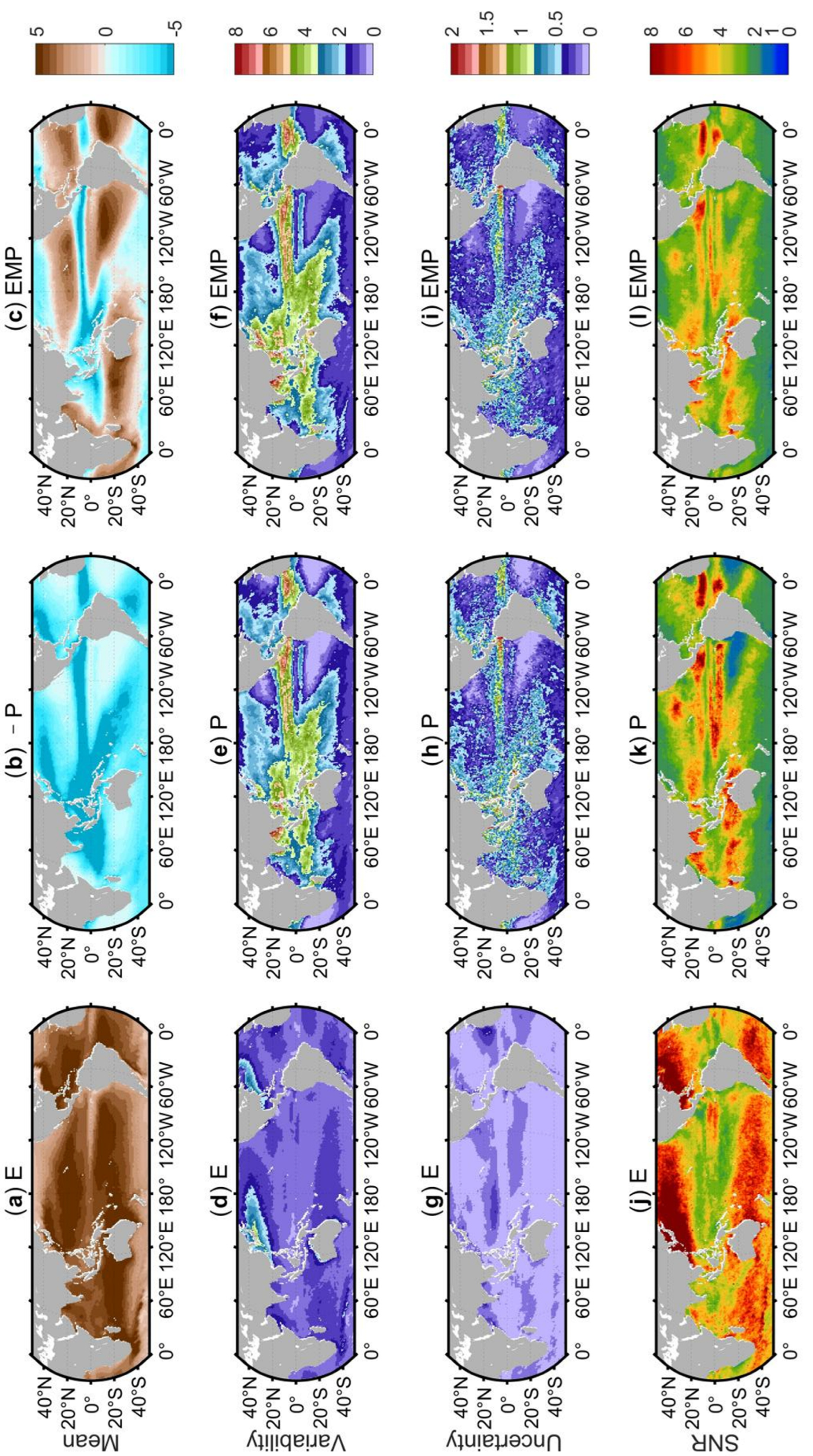
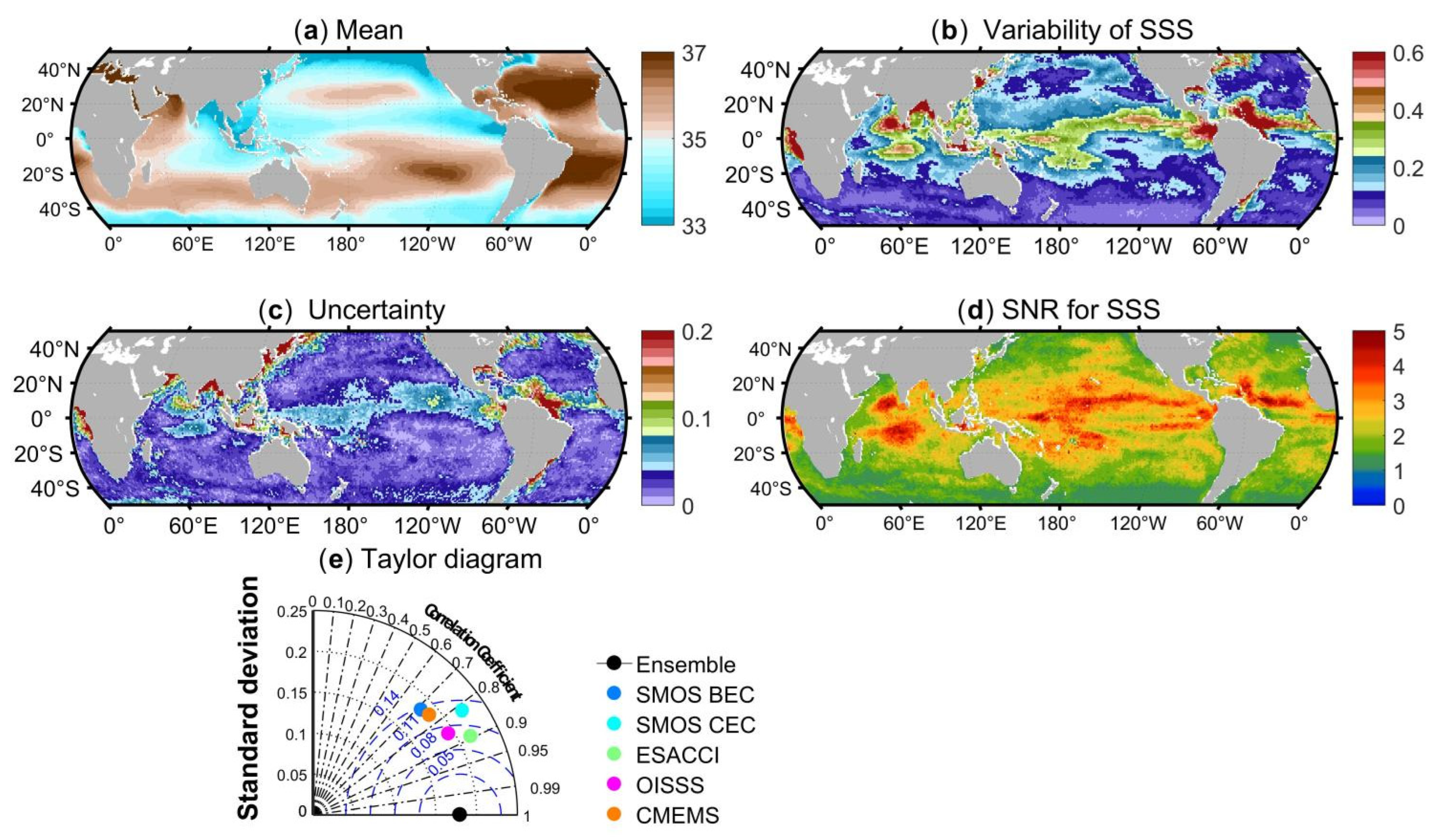
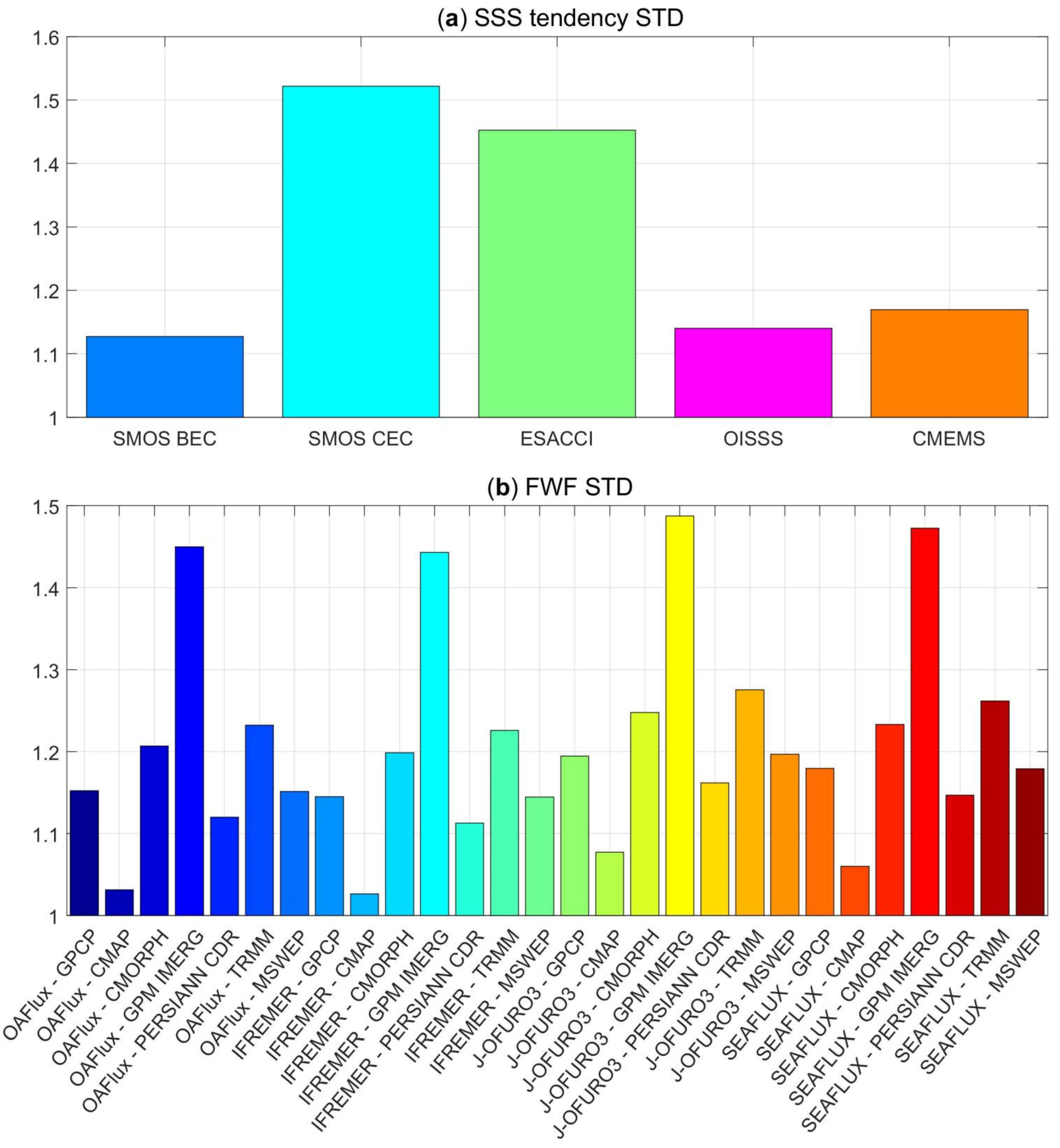
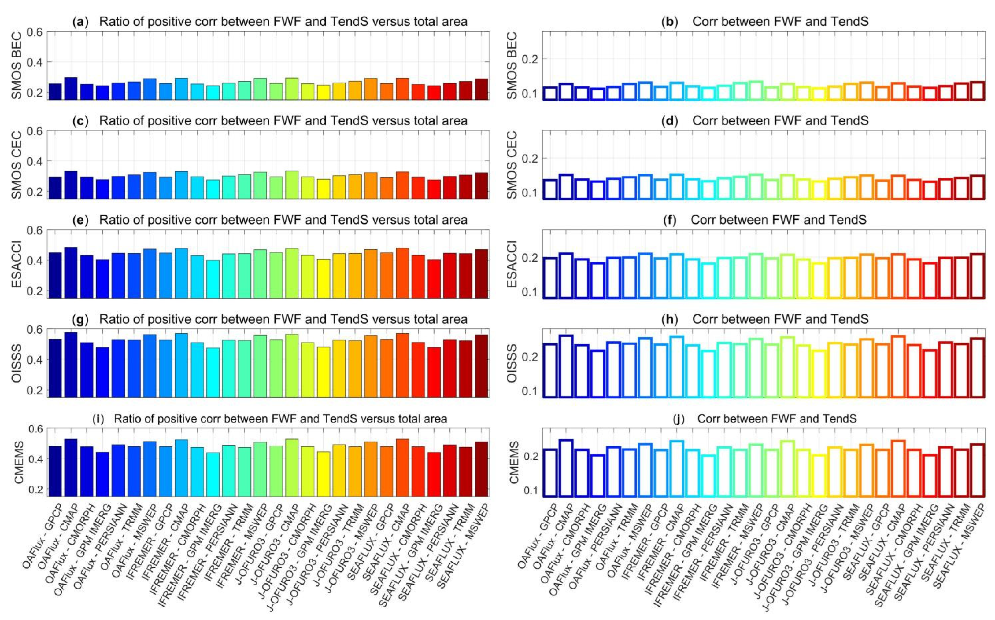
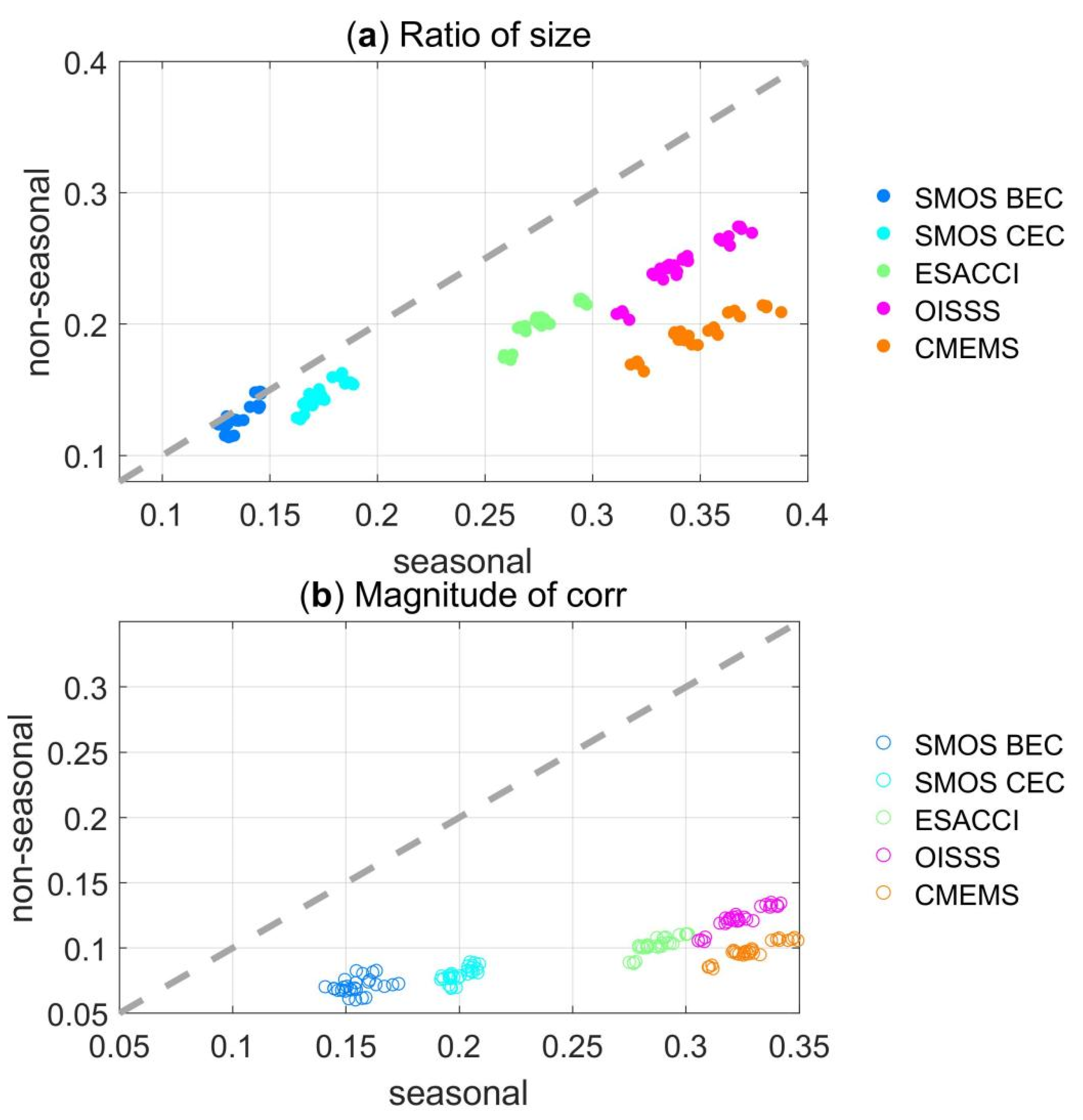
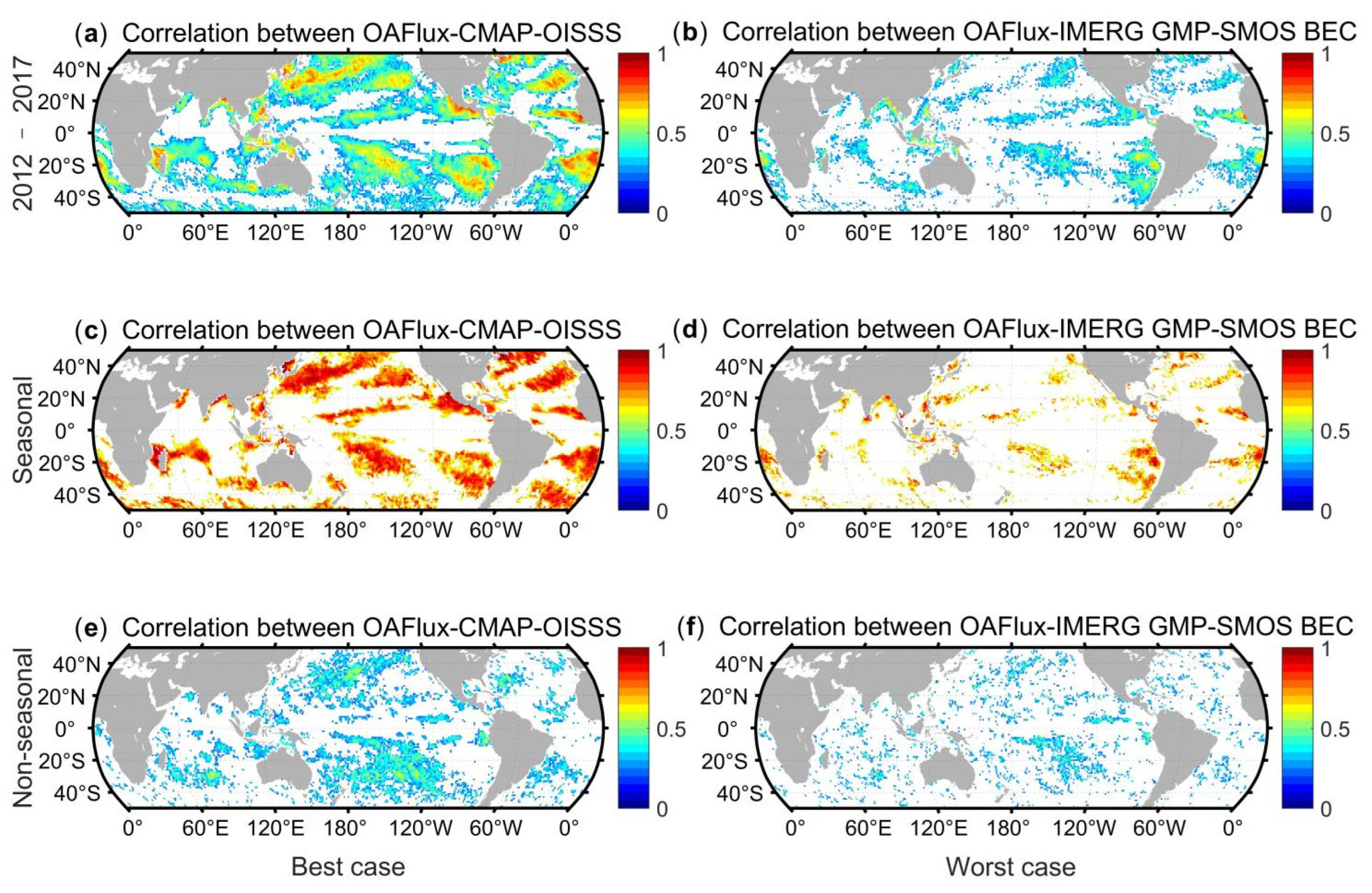
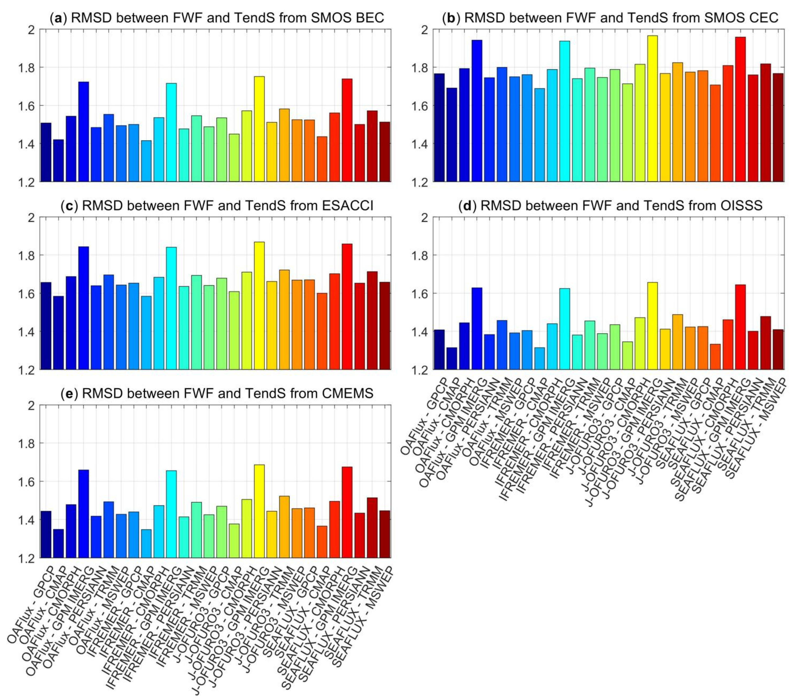
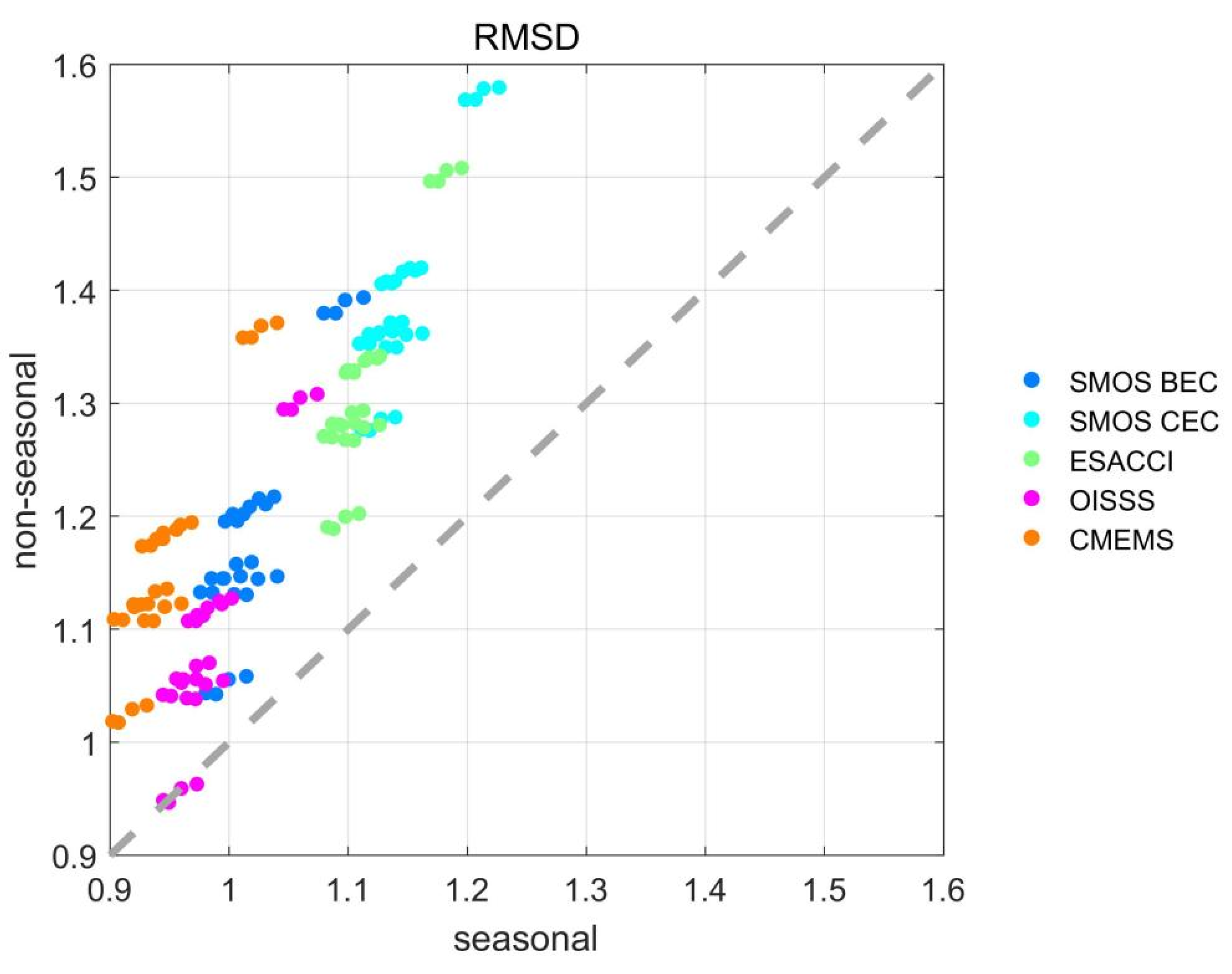
Table 1.
Main characteristics of the 7 , 4 and 5 SSS satellite-based products used in this study. Most products contain more sets of data with the different resolutions listed here. All data 1 are accessed on 20 April 2022.
Table 1.
Main characteristics of the 7 , 4 and 5 SSS satellite-based products used in this study. Most products contain more sets of data with the different resolutions listed here. All data 1 are accessed on 20 April 2022.
| Number | Datasets | Version | Variables | Resolution | Temporal Coverage | Reference |
|---|---|---|---|---|---|---|
| 1 | GPCP | Version 3.1 | 0.5°, monthly | January 1983–December 2019 | Huffman et al. [23] | |
| 2 | CMAP | Version2112blended | 2.5°, monthly | January 1979 to present | Xie et al. [27] | |
| 3 | CMORPH | Version 1 | 0.25°, daily | January 1998–December 2021 | Xie et al. [28] | |
| 4 | GPM IMERG | Version 6 | 0.1°, monthly | Jun 2000–September 2021 | Huffman et al. [29] | |
| 5 | PERSIANN CDR | None | 0.25°, monthly | January 1983 to present | Ashouri et al. [30] | |
| 6 | TRMM 3B42 | Version 7 | 0.25°, daily | January 1983–December 2019 | Huffman et al. [31] | |
| 7 | MSWEP | Version 2.8 | 0.1°, monthly | February 1979–November 2020 | Beck et al. [32], Beck et al. [33] | |
| 8 | OAFlux | Version 3 | 1°, monthly | January 1958–December 2020 | Yu and Weller [34] | |
| 9 | IFREMER | Version 4.1 | , | 0.25°, monthly | January 1992–December 2018 | Bentamy et al. [35] |
| 10 | J-OFURO3 | Version 1.1 | , | 0.25°, monthly | January 1988–December 2017 | Tomita et al. [36] |
| 11 | SEAFLUX | Version 3 | , | 0.25°, monthly | January 1988–December 2018 | Roberts et al. [37] |
| 12 | SMOS BEC | BEC, Level 4 Version 2 | 0.05°, daily | January 2011–December 2019 | Olmedo et al. [38] | |
| 13 | SMOS CEC | Version 7, Level 3 | 0.25°, 4 days | January 2010–November 2021 | Boutin et al. [39] | |
| 14 | ESA CCI | Version 03.21 | longitude 0.26°, latitude 0.2~1.5°, monthly | January 2010–September 2020 | Boutin et al. [40] | |
| 15 | OISSS | Version 1.0 | 0.25°, 4 days | August 2011–November 2021 | Melnichenko [41] | |
| 16 | CMEMS | MULTIOBS-GLO-PHY-S-SURFACE-MYNRT-015-013 | 0.25°, monthly | January 1993–December 2020 | Droghei et al. [42] |
1 Data can be downloaded from links in the data availability section. Some datasets need registration before access.
Publisher’s Note: MDPI stays neutral with regard to jurisdictional claims in published maps and institutional affiliations. |
© 2022 by the authors. Licensee MDPI, Basel, Switzerland. This article is an open access article distributed under the terms and conditions of the Creative Commons Attribution (CC BY) license (https://creativecommons.org/licenses/by/4.0/).
Share and Cite
MDPI and ACS Style
Liu, H.; Wei, Z.; Nie, X. Assessing the Relationship between Freshwater Flux and Sea Surface Salinity. Remote Sens. 2022, 14, 2149. https://doi.org/10.3390/rs14092149
AMA Style
Liu H, Wei Z, Nie X. Assessing the Relationship between Freshwater Flux and Sea Surface Salinity. Remote Sensing. 2022; 14(9):2149. https://doi.org/10.3390/rs14092149
Chicago/Turabian StyleLiu, Hao, Zexun Wei, and Xunwei Nie. 2022. "Assessing the Relationship between Freshwater Flux and Sea Surface Salinity" Remote Sensing 14, no. 9: 2149. https://doi.org/10.3390/rs14092149
Note that from the first issue of 2016, this journal uses article numbers instead of page numbers. See further details here.