
A Dual w-Test Based Quality Control Algorithm for Integrated IMU/GNSS Navigation in Urban Areas


Abstract
:
1. Introduction
2. Algorithm Design
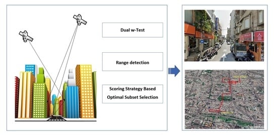
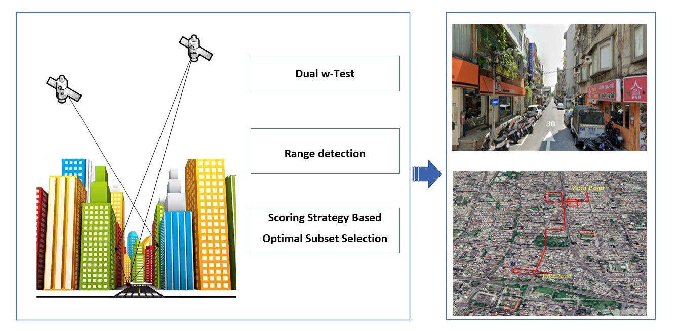
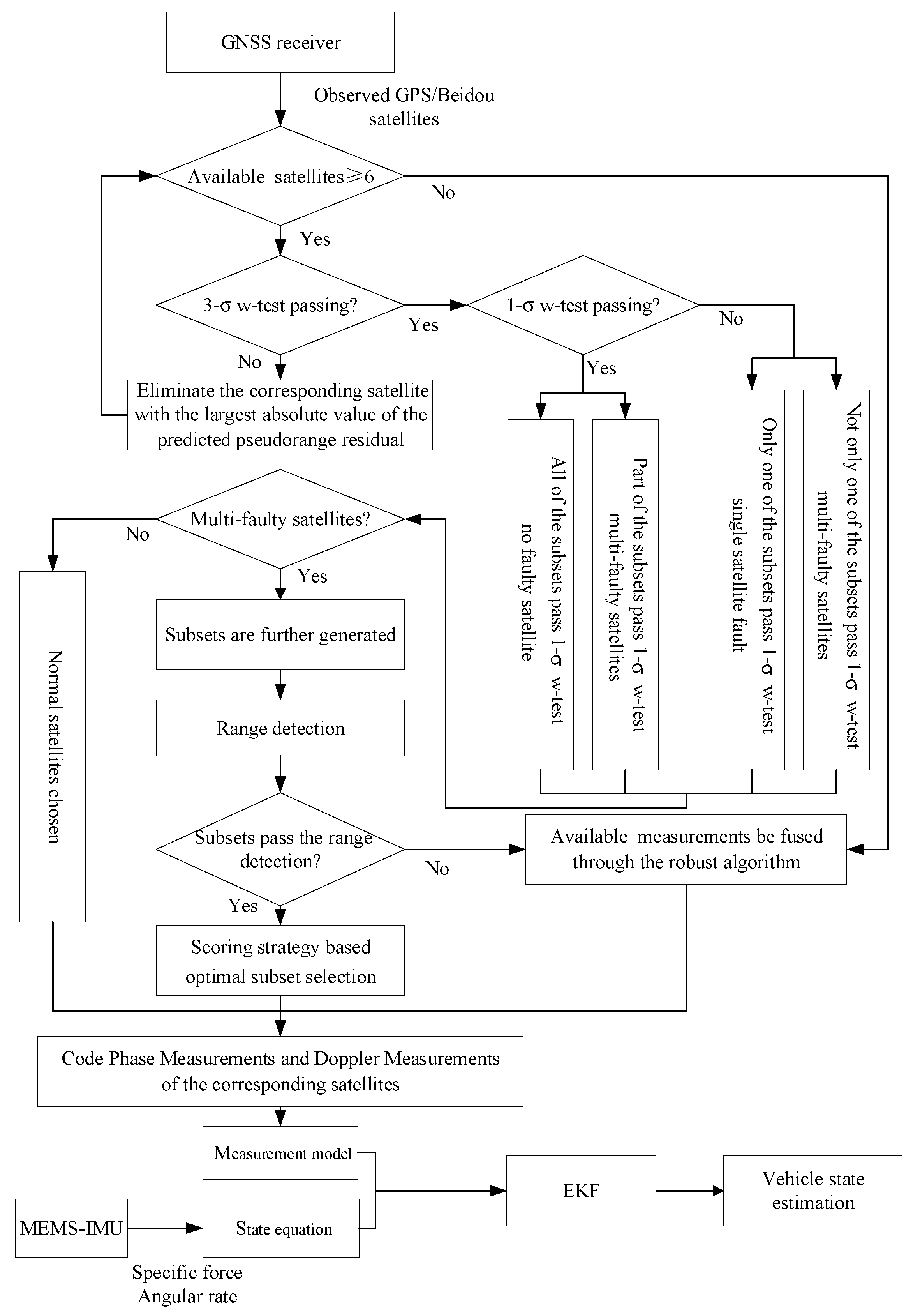
2.1. Dual w-Test
2.1.1. Traditional w-Test
2.1.2. and Dual w-Test
- The universal set and all subsets pass the w-test.
- The universal set and some subsets pass the w-test.
- The universal set does not pass the w-test, and only one of the subsets passes the w-test.
- The universal set does not pass the w-test, with more than one subset passing the w-test.
2.2. Scoring Strategy Based Optimal Subset Selection
2.3. IMU/GNSS Integration
3. Test and Validation
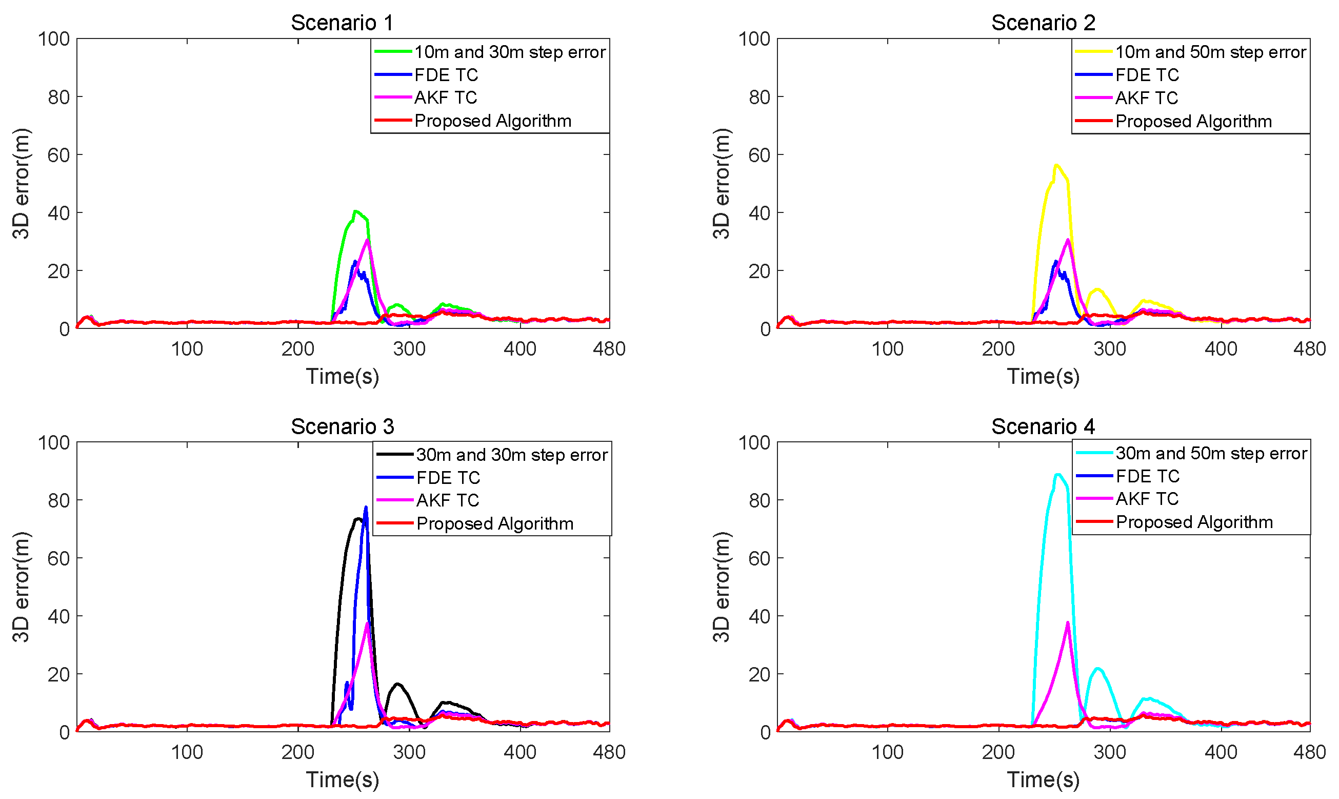
3.1. Simulation
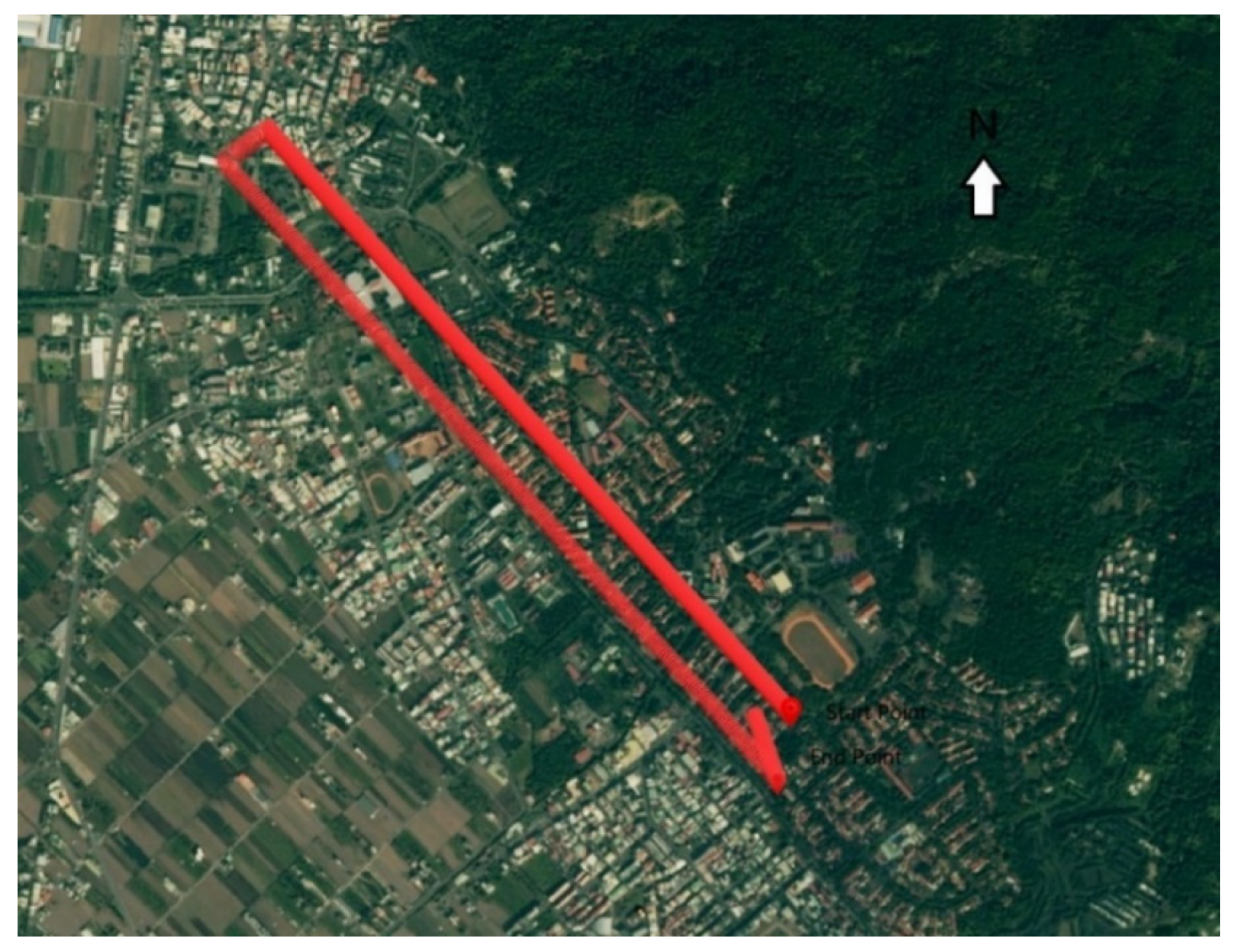
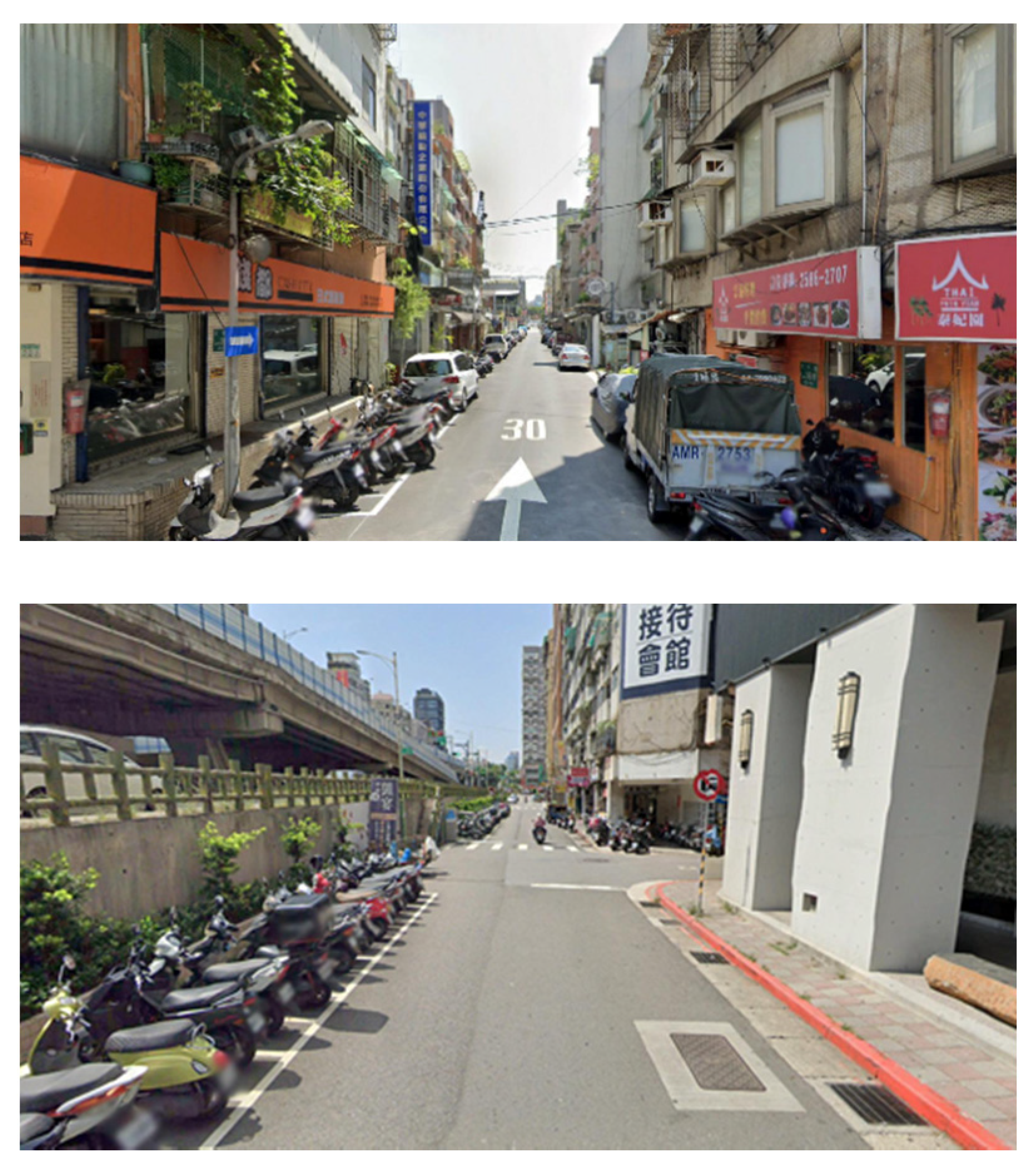
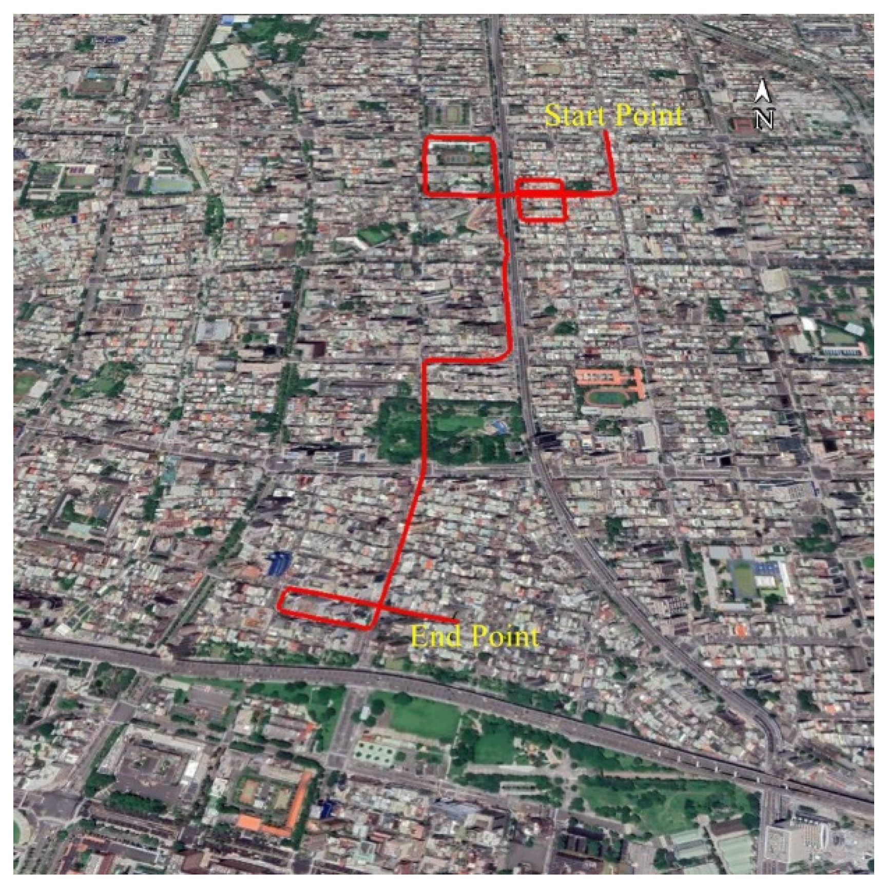
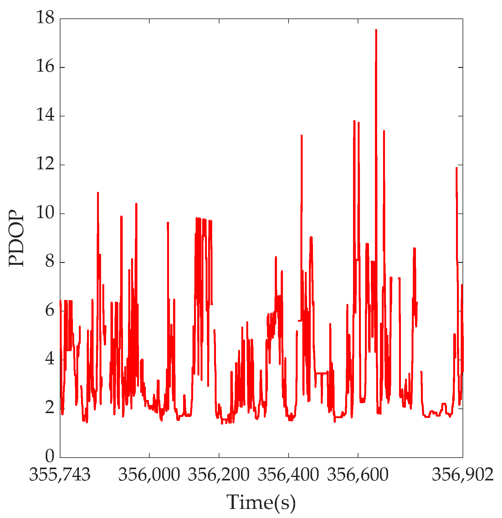
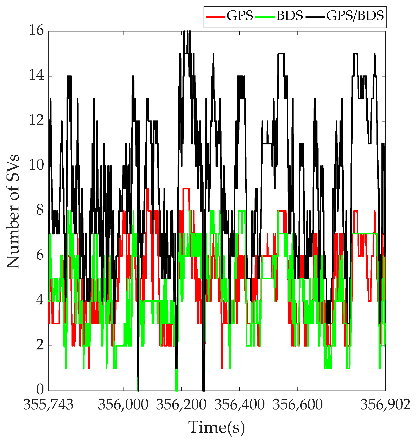
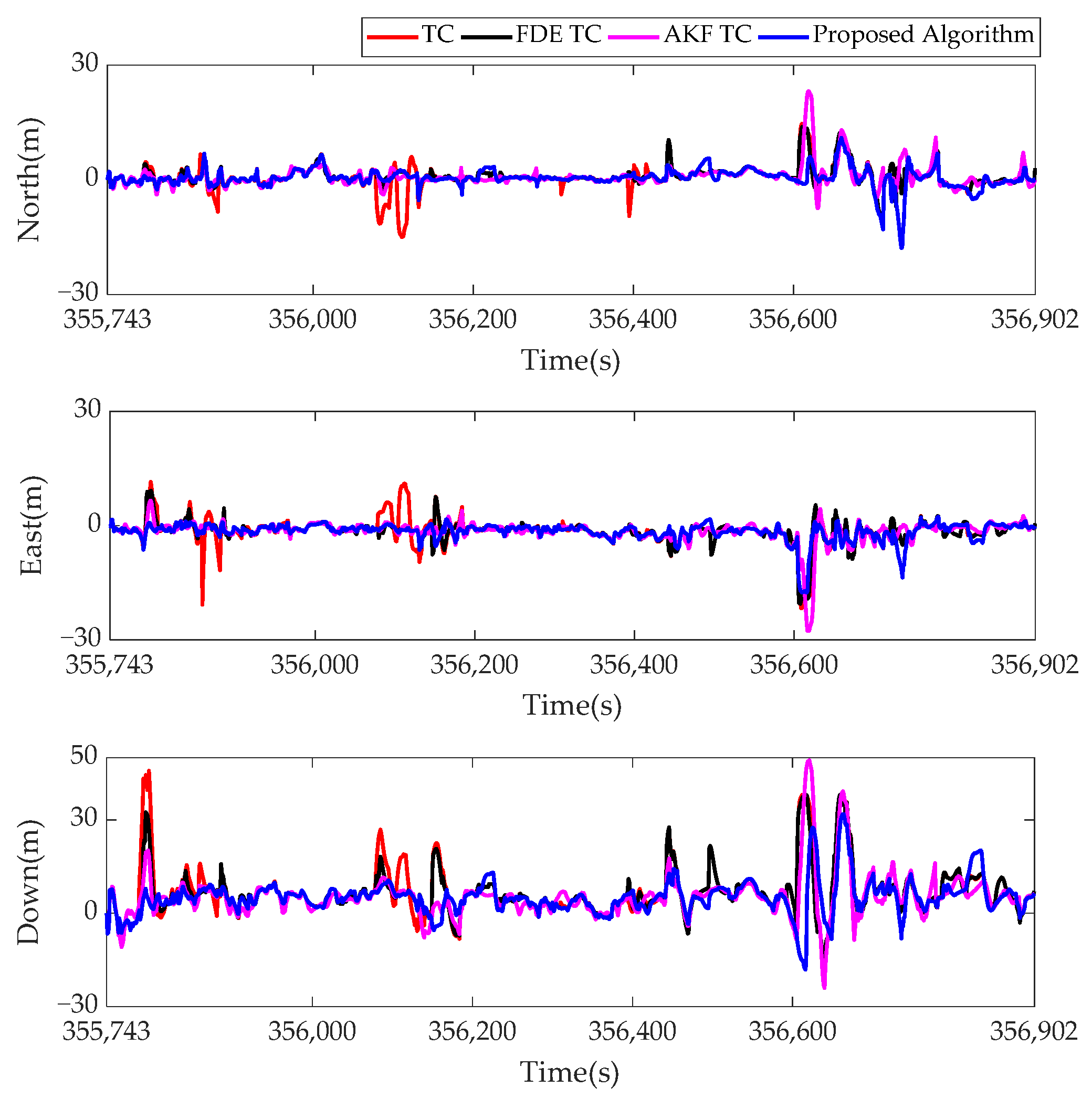
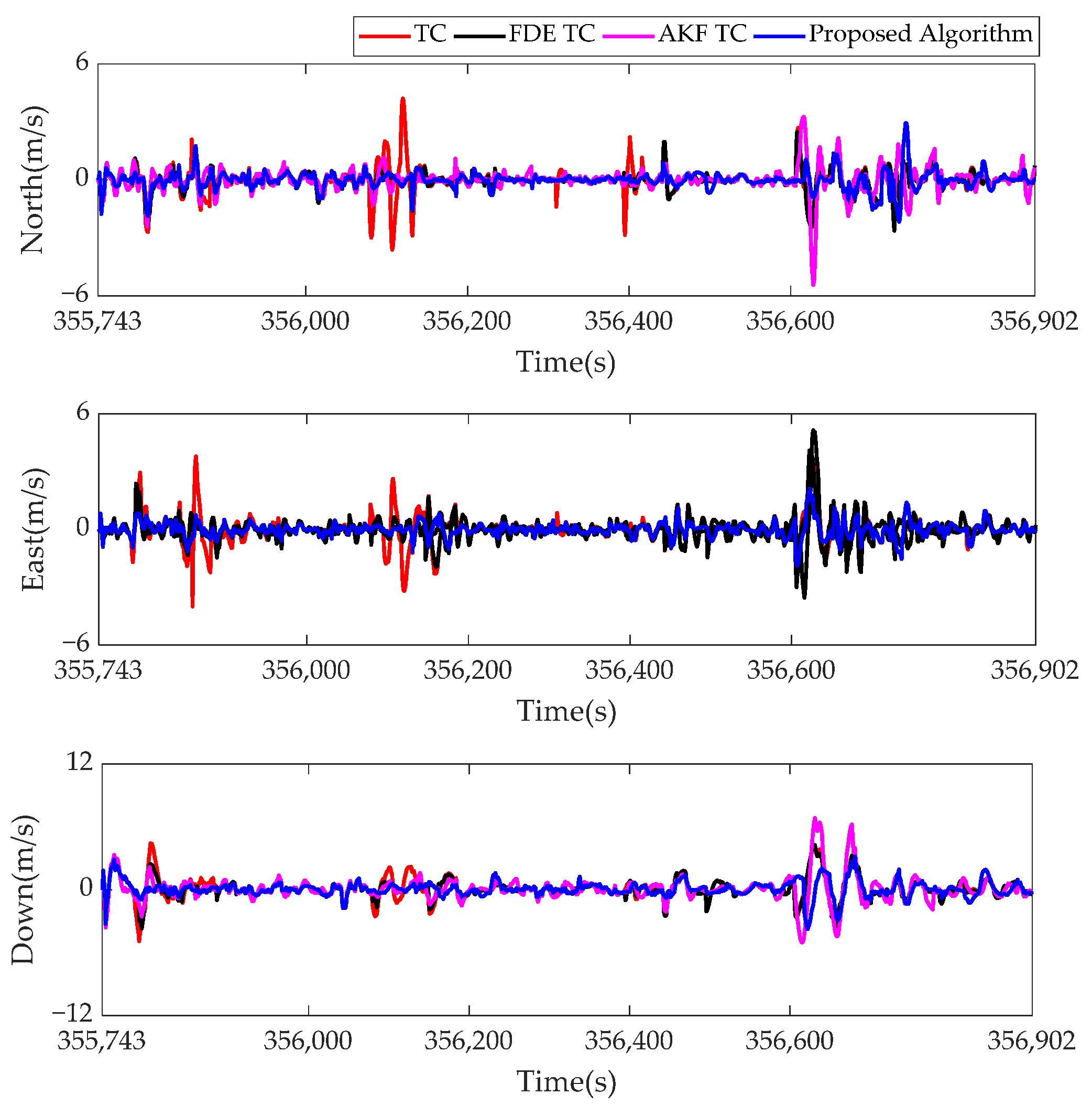
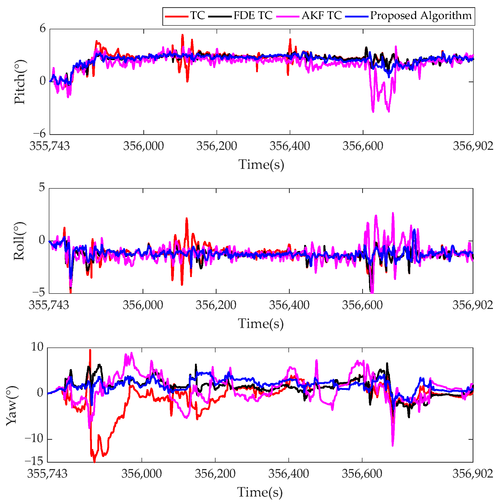
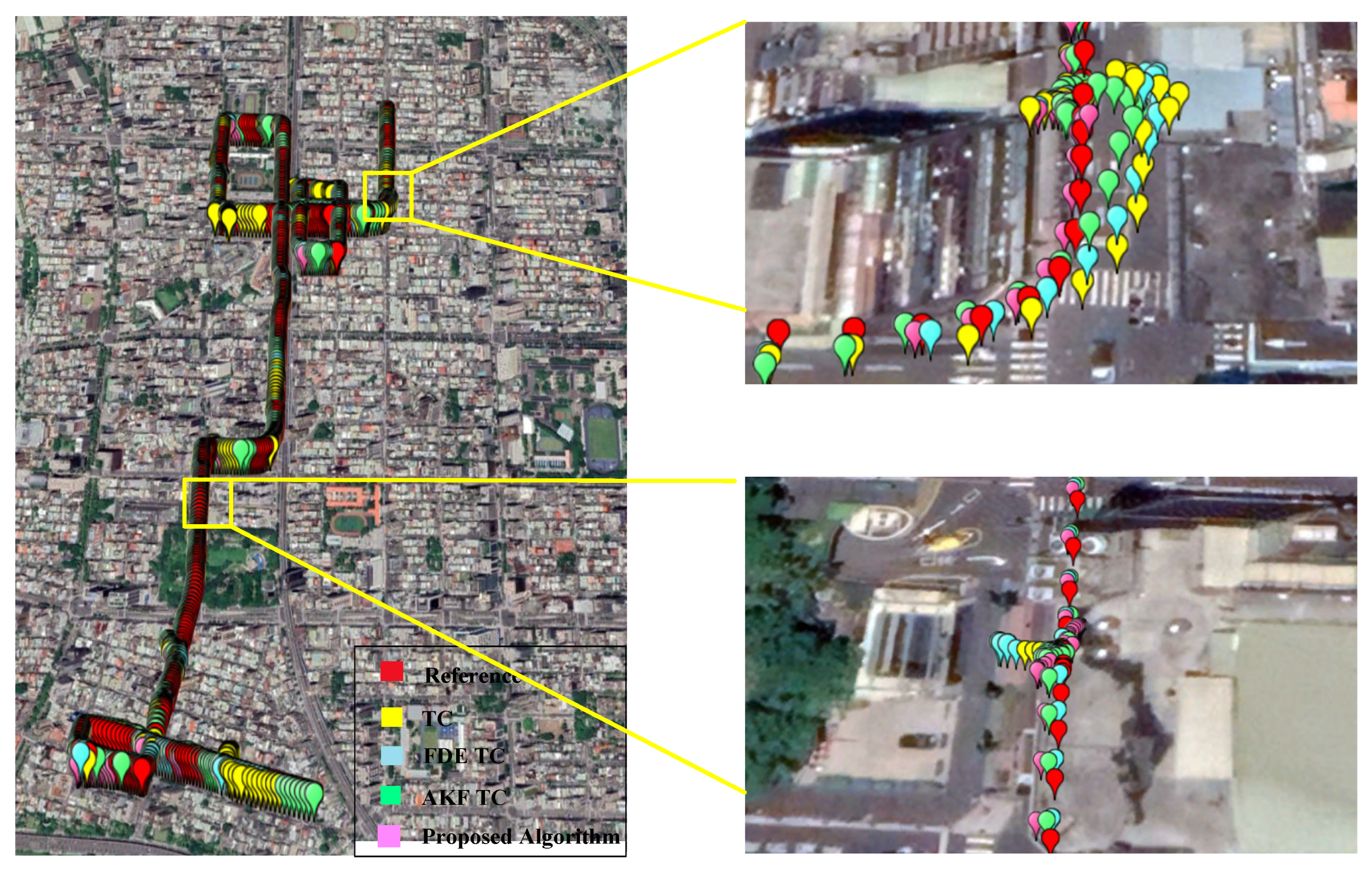
3.2. Field Test
4. Conclusions
Author Contributions
Funding
Conflicts of Interest
References
- Du, Y.; Wang, J.; Rizos, C.; El-Mowafy, A. Vulnerabilities and integrity of precise point positioning for intelligent transport systems: Overview and analysis. Satell. Navig. 2021, 2, 3. [Google Scholar] [CrossRef]
- Lee, Y.C. Analysis of range and position comparison methods as a means to provide GPS integrity in the user receiver. In Proceedings of the The User Recver Us Institute of Navigation Annual Meeting, Seattle, WA, USA, 24–26 June 1986; Volume 42, pp. 1–4. [Google Scholar]
- Parkinson, B.W.; Axelrad, P. A basis for the development of operational algorithms for simplified GPS integrity checking. In Proceedings of the Satellite Division’s First Technical Meeting, Colorado Spring, CO, USA, 21–25 September 1987. [Google Scholar]
- Sturza, M.A. Navigation system integrity monitoring using redundant measurements. Navigation 1988, 35, 483–501. [Google Scholar] [CrossRef]
- Brown, R.G.; Mcburney, P.W. Self-Contained GPS integrity check using maximum solution separation. Navigation 1988, 35, 41–53. [Google Scholar] [CrossRef]
- Virball, V.G.; Michalson, W.R. A GPS integrity channel based fault detection and exclusion algorithm using maximum solution separation. In Proceedings of the Position Location and Navigation Symposium, IEEE, Las Vegas, NV, USA, 11–15 April 1994. [Google Scholar]
- Hwang, P.Y.; Brown, R.G. RAIM-FDE revisited: A new breakthrough in availability performance with NIORAIM (novel integrity-optimized RAIM). Navigation 2006, 53, 41–52. [Google Scholar] [CrossRef]
- Lee, Y.C.; Fernow, J.P.; McLaughlin, M.P. GPS and Galileo with RAIM or WAAS for vertically guided approaches. In Proceedings of the 18th International Technical Meeting of the Satellite Division of the Institute of Navigation, Long Beach, CA, USA, 13–16 September 2005; pp. 302–326. [Google Scholar]
- Hewitson, S.; Wang, J. GNSS Receiver Autonomous Integrity Monitoring (RAIM) for multiple outliers. Eur. J. Navig. 2006, 4, 47–57. [Google Scholar]
- Knight, N.L.; Wang, J.; Rizos, C. GNSS integrity monitoring for two satellite faults. In Proceedings of the International Global Navigation Satellite Systems Society IGNSS Symposium 2009, Surfers Paradise, Australia, 1–3 December 2009. [Google Scholar]
- Joerger, M.; Stevanovic, S.; Chan, F.C.; Langel, S.; Pervan, B. Integrity risk and continuity risk for fault detection and exclusion using solution separation ARAIM. In Proceedings of the International Technical Meeting of the Satellite Division of the Institute of Navigation, Nashville, TN, USA, 16–20 September 2013. [Google Scholar]
- Bruggemann, T.S. GPS fault detection with IMU and aircraft dynamics. IEEE Trans. Aerosp. Electron. Syst. 2011, 47, 305–316. [Google Scholar] [CrossRef] [Green Version]
- Petovello, M.G. Real-Time Integration of a Tactical-Grade IMU and GPS for High-Accuracy Positioning and Navigation. Ph.D. Thesis, University of Calgary, Calgary, AB, Canada, 2003. [Google Scholar]
- Hewitson, S.; Wang, J. GNSS receiver autonomous integrity monitoring with a dynamic model. J. Navig. 2007, 60, 247–263. [Google Scholar] [CrossRef]
- Sun, R.; Wang, J.; Cheng, Q.; Mao, Y.; Ochieng, W.Y. A new IMU-aided multiple GNSS fault detection and exclusion algorithm for integrated navigation in urban environments. GPS Solut. 2021, 25, 147. [Google Scholar] [CrossRef]
- Mohamed, A.H.; Schwarz, K.P. Adaptive kalman filtering for INS/GPS. J. Geodesy. 1999, 73, 193–203. [Google Scholar] [CrossRef]
- Hide, C.; Moore, T.; Smith, M. Adaptive kalman filtering for lowc ost INS/GPS. J. Navig. 2003, 56, 143–152. [Google Scholar] [CrossRef]
- Xiao, Z.; Zhao, P.; Li, S. Adaptive fuzzy Kalman filter based on INS/GPS integrated navigation system. J. Chin. Inert. Technol. 2010, 18, 203. [Google Scholar]
- Xian, Z.; Hu, X.; Lian, J. Robust innovation-based adaptive Kalman filter for INS/GPS land navigation. In Proceedings of the Chinese Automation Congress, Changsha, China, 7–8 November 2013; pp. 374–379. [Google Scholar]
- Liu, Y.; Fan, X.; Lv, C.; Wu, J.; Li, L.; Ding, D. An innovative information fusion method with adaptive Kalman filter for integrated INS/GPS navigation of autonomous vehicles. Mech. Syst. Signal Process 2018, 100, 605–616. [Google Scholar] [CrossRef] [Green Version]
- Yan, F.; Li, S.; Zhang, E.; Chen, Q. An intelligent adaptive Kalman filter for integrated navigation systems. IEEE Access 2020, 8, 213306–213317. [Google Scholar] [CrossRef]
- Li, X.; Wang, X.; Liao, J.; Li, X.; Lyu, H. Semi-tightly coupled integration of multi-GNSS PPP and S-VINS for precise positioning in GNSS-challenged environments. Satell. Navig. 2021, 2, 1. [Google Scholar] [CrossRef]
- Li, X.; Wang, H.; Li, S.; Feng, S.; Wang, X.; Liao, J. GIL:a tightly coupled GNSS PPP/INS/LiDAR method for precise vehicle navigation. Satell. Navig. 2021, 2, 17. [Google Scholar] [CrossRef]
- Wang, H.; Li, H.; Zhang, W.; Zuo, J.; Wang, H. Derivative-free huber-kalman smoothing based on alternating minimization. Signal Process 2019, 163, 115–122. [Google Scholar] [CrossRef]
- Yang, Y.; Song, L.; Xu, T. Robust estimator for correlated observations based on bifactor equivalent weights. J. Geodesy 2002, 76, 353–358. [Google Scholar] [CrossRef]
- Yang, Y.; Cheng, M.K.; Shum, C.K.; Tapley, B.D. Robust estimation of systematic errors of satellite laser range. J. Geodesy 1999, 73, 345–349. [Google Scholar] [CrossRef]
- Yang, Y. Robust bayesian estimation. J. Geodesy 1991, 65, 145–150. [Google Scholar]
- Kuusniemi, H.; Wieser, A.; Lachapelle, G.; Takala, J. User-level reliability monitoring in urban personal satellite-navigation. IEEE Trans. Aerosp. Electron. Syst. 2007, 43, 1305–1318. [Google Scholar] [CrossRef]
- Teunissen, P. Quality control and GPS, chapter 7. In GPS for Geodesy, 2nd ed.; Springer: Berlin/Heidelberg, Germany, 1998. [Google Scholar]
- Sun, R.; Zhang, W.; Zheng, J.; Ochieng, W.Y. GNSS/INS integration with integrity monitoring for UAV No-fly zone management. Remote Sens. 2020, 12, 524. [Google Scholar] [CrossRef] [Green Version]
- Wu, F.; Nie, J.; He, Z. Classified adaptive filtering to GPS/INS integrated navigation based on predicted residuals and selecting weight filtering. Geomat. Inf. Sci. Wuhan Univ. 2012, 37, 261–264. [Google Scholar]
- Cheng, Q.; Chen, P.; Sun, R.; Wang, J.; Mao, Y.; Ochieng, W.Y. A new faulty GNSS measurement detection and exclusion algorithm for urban vehicle positioning. Remote Sens. 2021, 13, 2117. [Google Scholar] [CrossRef]


| Parameter | Initial Value |
|---|---|
| Scenarios | Time Interval of Faults (s) | Error Sources |
|---|---|---|
| 1 | 30 | 10 m, 30 m step errors added to the pseudoranges of two satellites |
| 2 | 30 | 10 m, 50 m step errors added to the pseudoranges of two satellites |
| 3 | 30 | 30 m, 30 m step errors added to the pseudoranges of two satellites |
| 4 | 30 | 30 m, 50 m step errors added to the pseudoranges of two satellites |
| Scenarios | TC | FDE TC | AKF TC | Proposed Algorithm | |||
|---|---|---|---|---|---|---|---|
| RMSE (m) | RMSE (m) | Improvement (%) | RMSE (m) | Improvement (%) | RMSE (m) | Improvement (%) | |
| 1 | 9.62 | 4.92 | 48.89 | 6.26 | 34.97 | 2.98 | 69.07 |
| 2 | 13.04 | 4.92 | 62.28 | 6.27 | 51.89 | 2.98 | 77.17 |
| 3 | 17.36 | 11.28 | 35 | 6.78 | 60.92 | 2.98 | 82.85 |
| 4 | 20.73 | 2.98 | 85.64 | 6.82 | 67.10 | 2.98 | 85.64 |
| Algorithm | RMSE (m) | |||
|---|---|---|---|---|
| North | East | 2D | Down | |
| TC | 3.31 | 3.72 | 4.98 | 10.79 |
| FDE TC | 2.65 | 3.15 | 4.11 | 9.66 |
| Improvement over TC (%) | 19.94 | 15.32 | 17.47 | 10.47 |
| AKF TC | 2.94 | 3.27 | 4.40 | 8.94 |
| Improvement over TC (%) | 11.18 | 12.10 | 11.65 | 17.15 |
| Proposed algorithm | 2.55 | 2.80 | 3.79 | 7.51 |
| Improvement over TC (%) | 22.96 | 24.73 | 23.90 | 30.40 |
| Improvement over FDE TC (%) | 3.77 | 11.11 | 7.79 | 22.26 |
| Improvement over AKF TC (%) | 13.27 | 14.37 | 13.86 | 15.88 |
| Algorithm | RMSE (m/s) | |||
|---|---|---|---|---|
| North | East | 2D | Down | |
| TC | 0.68 | 0.71 | 0.98 | 1.07 |
| FDE TC | 0.48 | 0.55 | 0.73 | 0.93 |
| Improvement over TC (%) | 29.41 | 22.54 | 25.51 | 13.08 |
| AKF TC | 0.63 | 0.63 | 0.89 | 1.21 |
| Improvement over TC (%) | 7.35 | 11.27 | 9.18 | −13.08 |
| Proposed algorithm | 0.45 | 0.38 | 0.59 | 0.72 |
| Improvement over TC (%) | 33.82 | 46.48 | 39.80 | 32.71 |
| Improvement over FDE TC (%) | 6.25 | 30.91 | 19.18 | 22.58 |
| Improvement over AKF TC (%) | 28.57 | 39.68 | 33.71 | 40.50 |
| Algorithm | RMSE (°) | ||
|---|---|---|---|
| Pitch | Roll | Yaw | |
| TC | 2.70 | 1.39 | 3.43 |
| FDE TC | 2.62 | 1.38 | 2.28 |
| Improvement over TC (%) | 2.96 | 0.72 | 33.53 |
| AKF TC | 2.33 | 1.43 | 3.08 |
| Improvement over TC (%) | 13.70 | −2.88 | 10.20 |
| Proposed algorithm | 2.58 | 1.27 | 2.25 |
| Improvement over TC (%) | 4.44 | 8.63 | 34.4 |
| Improvement over FDE TC (%) | 1.53 | 7.97 | 1.32 |
| Improvement over AKF TC (%) | −10.73 | 11.19 | 27.60 |
Publisher’s Note: MDPI stays neutral with regard to jurisdictional claims in published maps and institutional affiliations. |
© 2022 by the authors. Licensee MDPI, Basel, Switzerland. This article is an open access article distributed under the terms and conditions of the Creative Commons Attribution (CC BY) license (https://creativecommons.org/licenses/by/4.0/).
Share and Cite
Sun, R.; Qiu, M.; Liu, F.; Wang, Z.; Ochieng, W.Y. A Dual w-Test Based Quality Control Algorithm for Integrated IMU/GNSS Navigation in Urban Areas. Remote Sens. 2022, 14, 2132. https://doi.org/10.3390/rs14092132
Sun R, Qiu M, Liu F, Wang Z, Ochieng WY. A Dual w-Test Based Quality Control Algorithm for Integrated IMU/GNSS Navigation in Urban Areas. Remote Sensing. 2022; 14(9):2132. https://doi.org/10.3390/rs14092132
Chicago/Turabian StyleSun, Rui, Ming Qiu, Fei Liu, Zhi Wang, and Washington Yotto Ochieng. 2022. "A Dual w-Test Based Quality Control Algorithm for Integrated IMU/GNSS Navigation in Urban Areas" Remote Sensing 14, no. 9: 2132. https://doi.org/10.3390/rs14092132