Review

A Review of Multi-Sensor Fusion SLAM Systems Based on 3D LIDAR

1
College of Mechanical and Electrical Engineering, Hohai University, Changzhou 213022, China
2
Jiangsu Key Laboratory of Special Robot Technology, Hohai University, Changzhou 213022, China
3
College of Mechanical Engineering, Yangzhou University, Yangzhou 225127, China
*
Author to whom correspondence should be addressed.
These authors contributed equal to this work.
Remote Sens. 2022, 14(12), 2835; https://doi.org/10.3390/rs14122835
Submission received: 5 May 2022 / Revised: 10 June 2022 / Accepted: 10 June 2022 / Published: 13 June 2022

Abstract

:
The ability of intelligent unmanned platforms to achieve autonomous navigation and positioning in a large-scale environment has become increasingly demanding, in which LIDAR-based Simultaneous Localization and Mapping (SLAM) is the mainstream of research schemes. However, the LIDAR-based SLAM system will degenerate and affect the localization and mapping effects in extreme environments with high dynamics or sparse features. In recent years, a large number of LIDAR-based multi-sensor fusion SLAM works have emerged in order to obtain a more stable and robust system. In this work, the development process of LIDAR-based multi-sensor fusion SLAM and the latest research work are highlighted. After summarizing the basic idea of SLAM and the necessity of multi-sensor fusion, this paper introduces the basic principles and recent work of multi-sensor fusion in detail from four aspects based on the types of fused sensors and data coupling methods. Meanwhile, we review some SLAM datasets and compare the performance of five open-source algorithms using the UrbanNav dataset. Finally, the development trend and popular research directions of SLAM based on 3D LIDAR multi-sensor fusion are discussed and summarized.

1. Introduction

A mobile robot is a complex system integrating computer technology, sensor technology, information processing, electronic engineering, automation, and artificial intelligence. With the assistance of artificial intelligence technology, mobile robots with versatile functions are widely used in the fields of emergency rescue, industrial automation, and smart life. Precise positioning is one of the key technologies for mobile robots to complete tasks autonomously. With the rapid development of robot technology, a single sensor can no longer meet the increasingly rich functional requirements of robots. Therefore, the technology of information fusion of multi-source sensing has gradually attracted attention.
Mobile robots are widely used in indoor environments. 2D LIDAR has become the choice for indoor navigation and positioning due to the advantages of high-precision ranging and reduced data volume. However, with the increasing demand for outdoor scenes, robots are gradually moving towards increasingly complex open scenes. Driven by the DARPA (Defense Advanced Research Projects Agency Ground Challenge) [1,2], multi-line 3D LIDAR became known and began to be widely used in outdoor scenes. 3D LIDAR has stronger environmental awareness but at the cost of expensive price, high data volume, and processing difficulty. In recent years, with the popularization of 3D LIDAR and the enhancement of the computing power of embedded processors, the positioning technology based on 3D LIDAR has developed rapidly. 3D LIDAR provides high-density point clouds with richer matching methods and better robustness for the matching between frames. Furthermore, it can be fused with image and odometer information [3] to enhance the positioning accuracy, which has become the mainstream sensor used in many fields such as unmanned driving, robot autonomous navigation, and drone flight control.
For a SLAM system, accurate position and orientation estimation are essential. Scholars have conducted a lot of studies, including vision-based methods and LIDAR-based methods, to realize real-time high-precision 6-DOF state estimation for mobile robots. However, a single sensor system has limitations. On the one hand, the dependence of vision on initialization and the sensitivity to the sum of illumination leads to the instability of the system. On the other hand, the sparse information provided by LIDAR rapidly degenerates the positioning in unstructured scenes. In addition, the rapid motion mode and long-term error accumulation further invalidates the odometer. Therefore, many auxiliary sensors such as IMU, GPS, MEMS, and UWB are added to the positioning system to solve the above problems. In recent years, there have been many LIDAR SLAM review literatures. Most of them introduce the development process of the entire 3D LIDAR SLAM in simple terms, which includes huge but too complicated content.
Tee [4] presents a detailed analysis and comparison of several common open-source solutions for 2D SLAM. The advantages and disadvantages of each method are demonstrated by simulation and experiment. However, 3D SLAM has not been addressed. Bresson [5] reviews LIDAR SLAM related to the large-scale problem faced by autonomous driving. Similarly, reference [6] is an earlier SLAM review, which discusses in detail the basic issues of SLAM and many works in the development of SLAM, including long-distance SLAM, theoretical performance analysis, semantic association, and development directions. Both works summarize the classic theories and work in the field of SLAM, however, the related content of multi-sensor fusion is not involved.
Debeunne [7] divides SLAM into three parts: image-based, LIDAR-based, and image- LIDAR fusion. The integration of SLAM work, complicated integration methods, and the development process of data fusion have not been mentioned. Taheri [8] proposes a SLAM review showing the development of SLAM by reviewing important works. It summarizes and looks forward to SLAM work from multiple directions and stages. However, this work mainly summarizes the visual SLAM, and the reference value of LIDAR SLAM is limited. Zhou [9] summarizes the SLAM algorithm based on 3D LIDAR from the aspects of optimization framework, key SLAM modules, and future research hotspots. Subsequently, this work compares the performance of various SLAM algorithms in detail, which has high reference value.
It can be seen that most of the relevant reviews of SLAM are based on key modules such as front-end matching, closed-loop detection, back-end optimization, and mapping, focusing on the development history and latest works of SLAM. This paper will summarize the multi-sensor fusion SLAM algorithms based on 3D LIDAR from different perspectives. The contributions are:
  • The multi-sensor fusion SLAM systems in recent years are categorized and summarized according to the types of fused sensors and the means of data coupling.
  • This work fully demonstrates the development of multi-sensor fusion positioning and reviews the works of both loosely coupled and tightly coupled systems, so as to help readers better understand the development and latest progress of multi-sensor fusion SLAM.
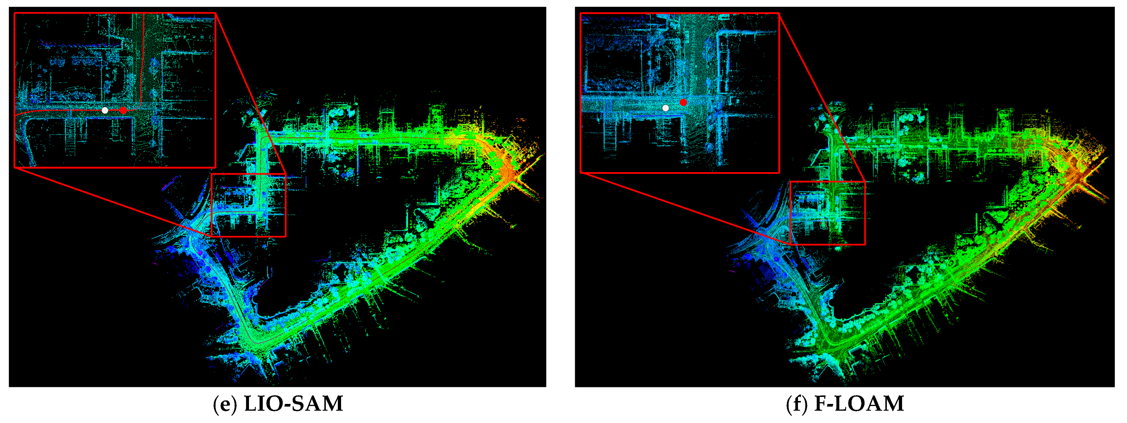
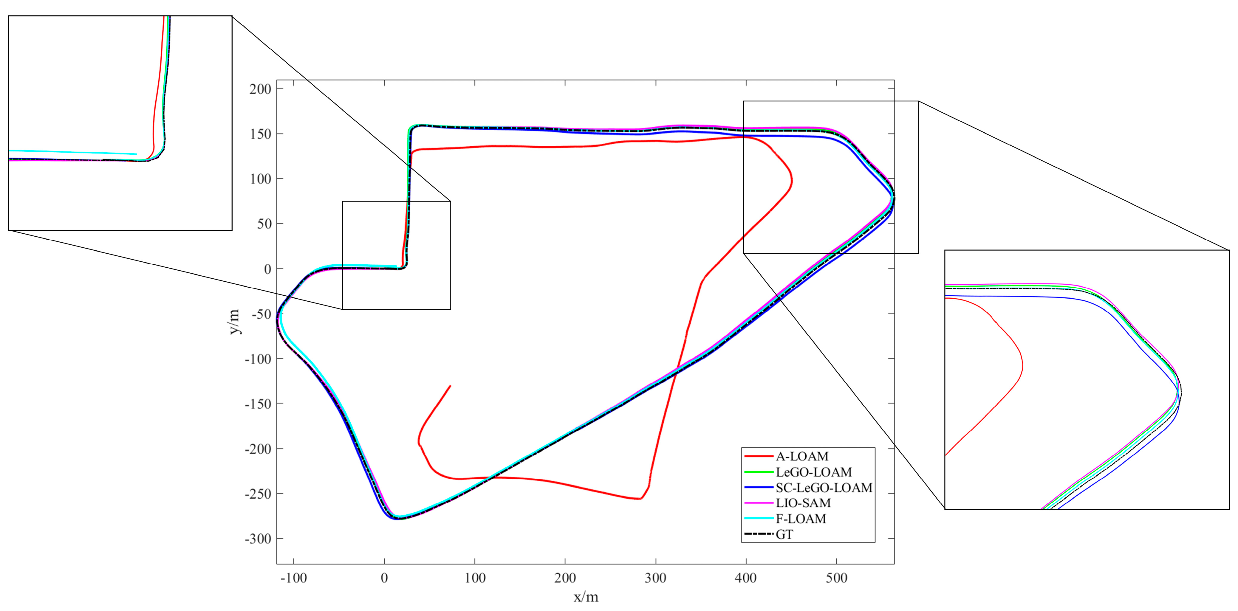
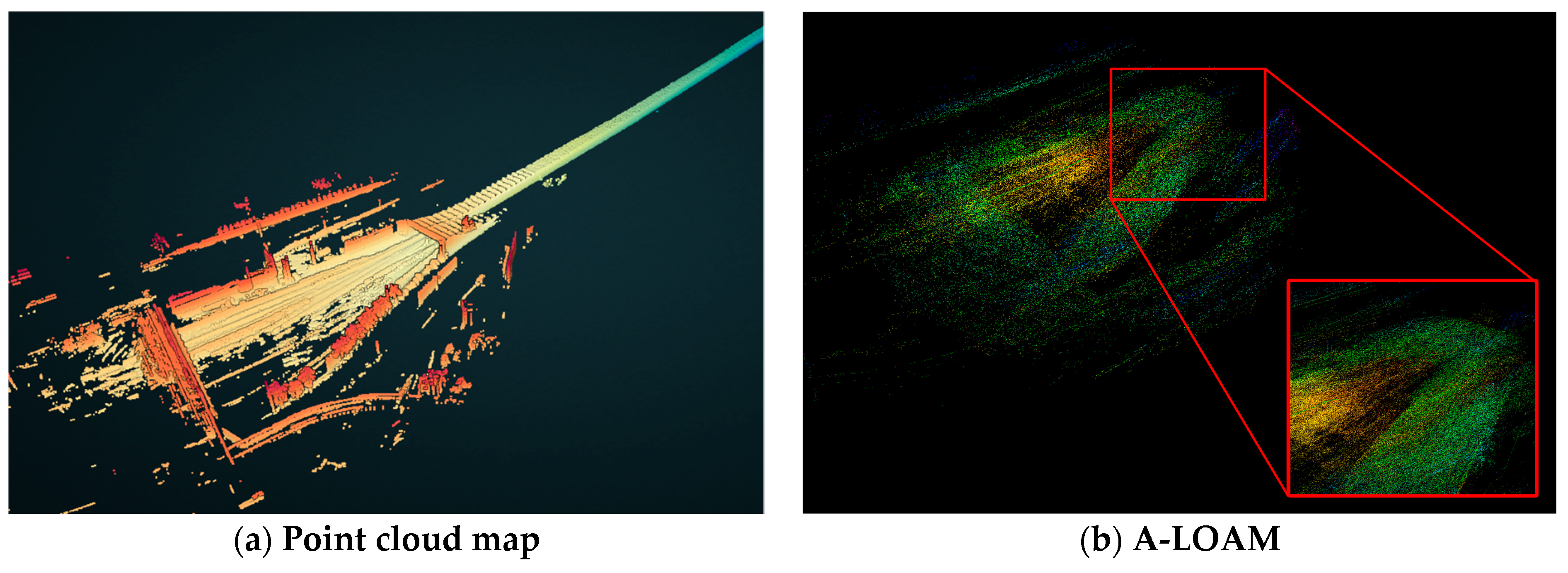
  • This paper reviews some SLAM datasets and compares the performance of five open-source algorithms using the UrbanNav dataset.
This paper provides a detailed overview of multi-sensor systems through five main sections. The first section details the necessity of multi-sensor fusion in localization systems. In Section 2, the basic problems to be solved by SLAM and the classical framework are presented. In Section 3, the related works of the loosely coupled system are reviewed in detail in two parts according to the sensor types. Similarly, the related works on tightly coupled systems are reviewed in Section 4. A comparison table is given at the end of each section. Finally, a summary of the full text and an outlook for the follow-up works are presented. Abbreviations used in this paper are summarized in Table 1.

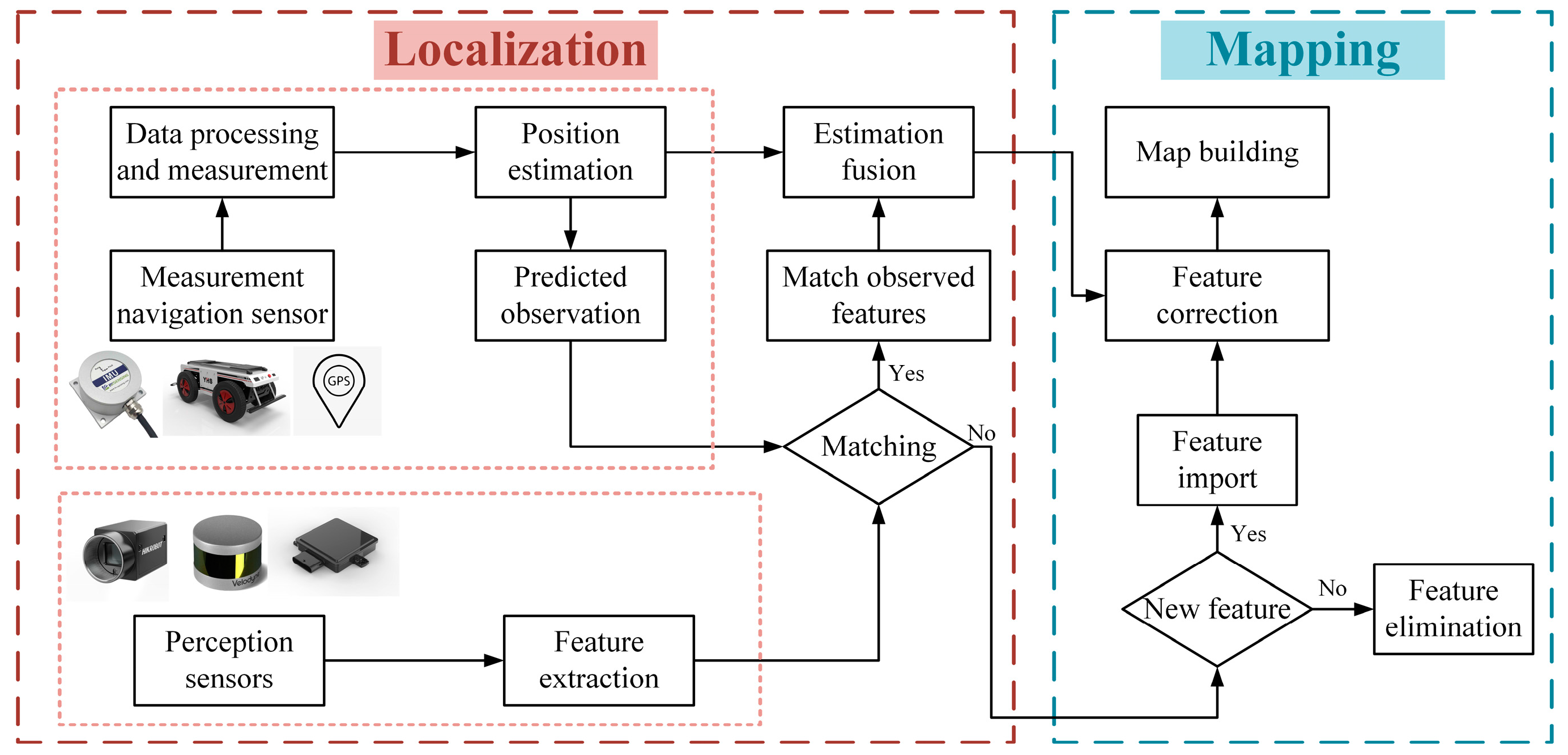
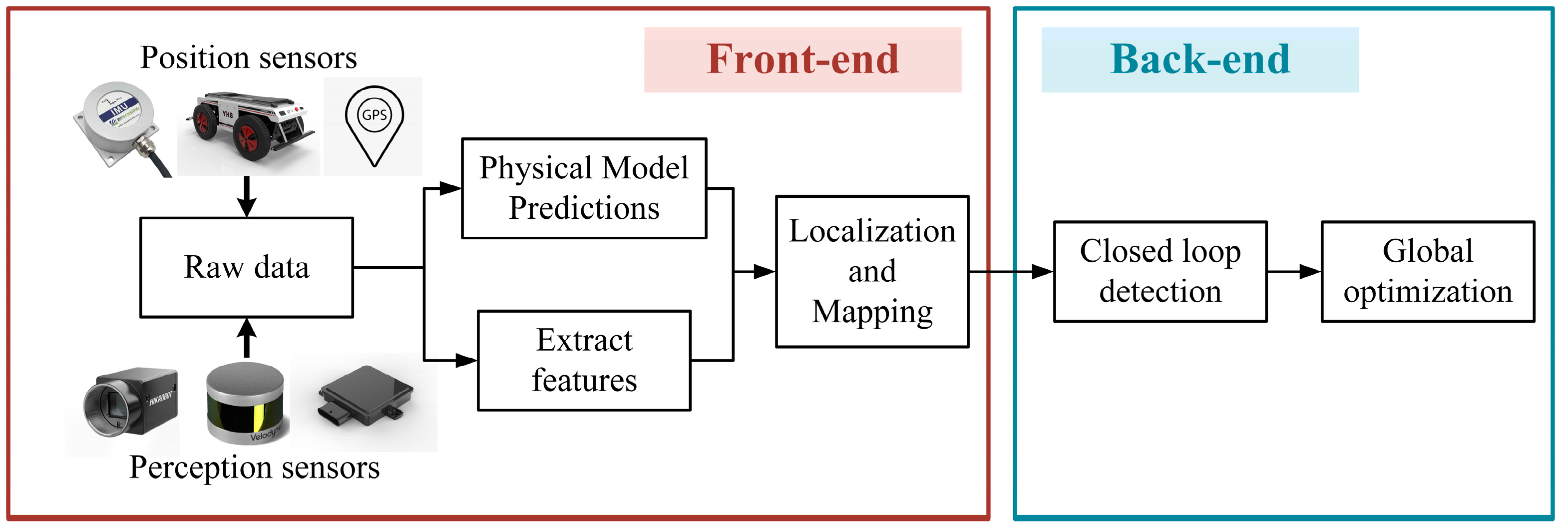
2. Simultaneous Localization and Mapping System

Over the past few decades, SLAM techniques have come a long way. SLAM systems based on various sensors have been developed, such as LIDAR, cameras, millimeter-wave radar, ultrasonic sensors, etc. As early as in 1990, the feature-based fusion SLAM framework [10], as shown in Figure 1, was established and it is still in use today. The SLAM problem has evolved from two independent modules, localization and mapping, into a complete system that integrates the two. The two modules promote each other. The high-precision odometer composed of multiple sensors provides real-time pose estimation for the robot and the basis for the reconstruction and stitching of the 3D scene. Similarly, high-precision 3D reconstruction provides important data for pose estimation for feature-based odometry. Even a separate odometer system is also inseparable from the establishment or storage of temporary local maps to assist pose estimation.
Most modern SLAM systems are divided into two parts: front end and back end (as shown in Figure 2). The front end is responsible for estimating the current frame pose in real time and storing the corresponding map information. The back end is responsible for large-scale pose and scene optimization. Loop closure detection is one of the key issues of SLAM, which helps the robot identify visited scenes and trigger global-scale drift correction. Large-scale global optimization is also the main difference between SLAM and modern odometry. The two methods have many similarities in pose estimation. Most modern multi-sensor fusion technologies act in the front end to achieve high-precision and low drift of the odometer systems by the means of information complementation, local pose fusion, and multi-data source filtering.
The development of single sensor system is relatively mature, among which LIDAR, camera, and IMU are the most common sensors in SLAM systems. 3D LIDAR can provide the system with rich structural information of the environment. However, the data are discrete and numerous. The camera can capture color and texture in the environment at high speed, but depth cannot be directly perceived by the camera and it tends to be perturbed by light. The IMU can sensitively perceive weak changes of the system in a very short period of time, but long-term drift is inevitable. The characteristics of the three are distinct, and their advantages and disadvantages are obvious. Single-sensor SLAM systems are fragile and full of uncertainty. They are not capable of dealing with multiple complex environments such as high-speed scenes, small spaces, and open and large scenes at the same time.
Therefore, multi-sensor fusion has become a new trend in the development of SLAM systems. Most of the SLAM and odometry systems for multimodal sensor fusion use a combination of LIDAR, camera, and IMU, which can be categorized as loosely coupled or tightly coupled modes. The loosely coupled system processes measurement data of each sensor separately and fuses them in a filter that marginalizes data of the current frame to achieve the latest state estimation results. The tightly coupled system jointly optimizes the measurement data of all sensors and combines the observation characteristics and physical models of each sensor to obtain a more robust pose estimation. The loosely coupled system has the advantages of small calculation amount, simple system structure, and easy implementation. However, its positioning accuracy usually has limitations. In contrast, a tightly coupled system is computationally intensive so that its implementation is difficult, but it gains a more accurate state estimation in complex and changeable environments.
Based on these three sensors, a number of multi-sensor fusion simultaneous localization and mapping works have emerged in recent years. In this paper, according to the coupling method of the system and the types of sensors to be fused, these works are divided into LIDAR-IMU loosely coupled system, Visual-LIDAR-IMU loosely coupled system, LIDAR-IMU tight coupled system, and Visual-LIDAR-IMU tight coupled system. The development of SLAM is a process of transition from loose coupling to tight coupling. The classification of some of the SLAM systems mentioned in this paper and the developmental relationship between them are shown in Figure 3.

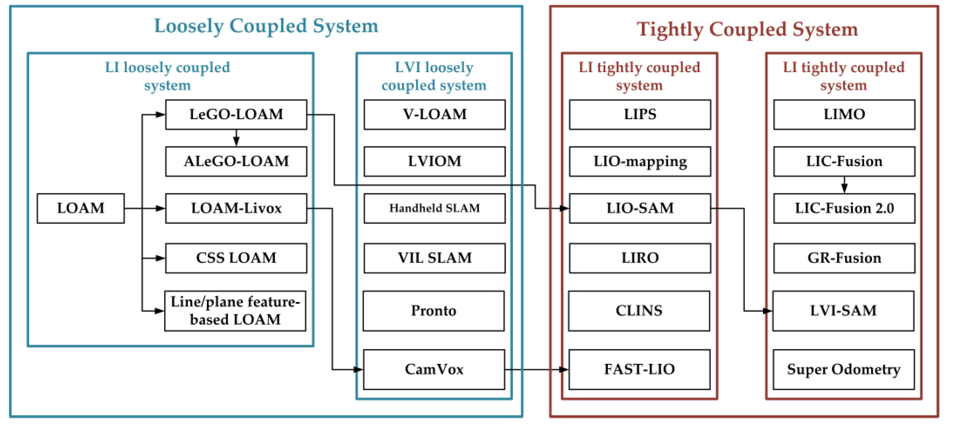
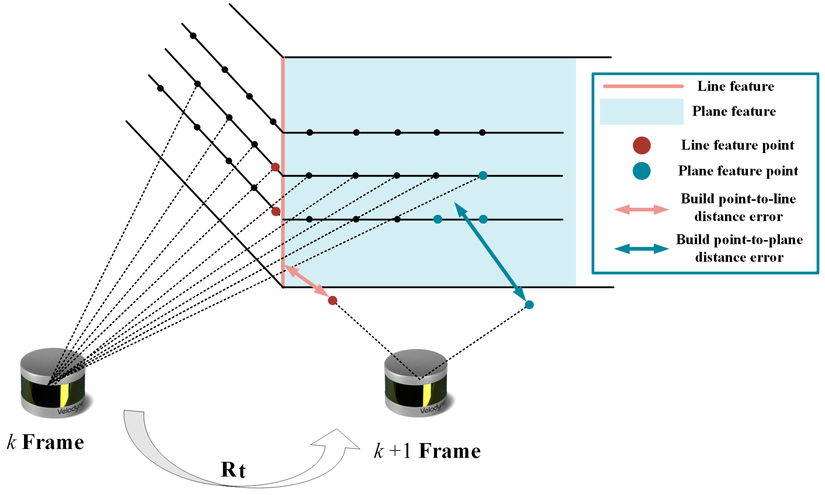
3. Multi-Sensor Loosely Coupled System Based on LIDAR

The emergence of loosely coupled systems has opened up a new stage in the development of multi-sensor fusion systems. Until now, its application in low-cost platforms with limited computation powers is still wide. Loose coupling is mostly applied in three aspects: multi-sensor-based stage pose estimation, raw data-based information complementarity, and sensor-assisted pose constraints.

3.1. LIDAR-IMU Loosely Coupled System

Most loosely coupled systems appear in earlier works. The popularity and wide attention of LIDAR-based 3D SLAM technology can be attributed to Zhang’s original work, the LOAM algorithm [11]. One of his important contributions was to extract the information of effective edge and plane feature points from the complex point cloud. Furthermore, the point-to-line and plane distances are used to construct an error function and solve the nonlinear optimization problem of the pose, as shown in Figure 4. Even the earliest LIDAR SLAM systems already had the concept of sensor fusion. This work uses the integration operation of the gyroscope and accelerometer of the six-axis IMU to obtain the prior pose, which further improves the accuracy of the LIDAR odometer. However, LOAM does not have loop closure detection and global pose optimization at the back-end. After that, many LIDAR-IMU loosely coupled systems were improved and perfected on the basis of LOAM. The work presented in this section not only focuses on sensor data fusion, but also improving the point cloud registration of the front end and the overall optimization of the back end.
Shan [12] proposed the LeGO-LOAM algorithm on the basis of LOAM, which introduced point cloud clustering and ground segmentation into data preprocessing to speed up point cloud registration [13]. At the same time, a simple acceleration formula is used to process the IMU data for point cloud distortion correction and provide a priori pose. The IMU has played the same role in line/plane feature-based LOAM and two-stage LOAM. The feature extractions have drawn more attention. The normal vector of point is used to extend the feature types in both methods [14,15]. Different from both of the above methods, CSS-based LOAM and ALeGO-LOAM enhance the feature quality of LOAM [16,17]. Since the curvature scale space method and adaptive cloud sampling method are put forward, more accuracy edge points and plane points are extracted. However, this loose integration method does not effectively exclude the influence of the measurement bias of the IMU itself. Moreover, the IMU is merely a supplementary means.
In addition to the improvement in feature extraction, improved ICP and GPU acceleration are also optimized. ICP is widely used in SLAM front end. Many works in recent years have proposed faster and more robust ICP variants in order to guarantee the real-time (10 Hz) performance of LIDAR odometry in real-life regularization scenarios. The latest work [18] introduces symmetric KL divergence in the front end ICP algorithm. Its optimization object includes not only the distance between points, but also the difference in distribution shape. In order to ensure the real-time performance and calculation accuracy of the front end, GPU acceleration is applied to point cloud computing including SuMa [19], Elastic-LiDAR Fusion [20], and Droeschel [21]. The shape of the distance data is approximated as a set of disks called Surfel [22], which is convenient for solving point-to-plane problem in GPU. Due to GPU acceleration, the dense point cloud is exhibited in front of people. The visual content is more understandable. To some extent, these point clouds have semantic meaning. Moreover, these methods can be used in virtual reality and augmented reality. However, portable devices and mobile robots still lack powerful GPUs.
It is essential to adopt overall optimization of the back end for the SLAM system. In the latest work [23], Yue enriched feature types. He used the Multi-metric Linear Least Squares Iterative Closest Point (MULLS ICP) algorithm based on categorical feature points to efficiently estimate self-motion and construct a submap-based PGO (Pose Graph Optimization) backend optimization. Effective loop closure detection is a significant procedure of SLAM. In [24,25], the geometric and intensity information of the point cloud are encoded, and a global point cloud descriptor is set to implement a rotation-invariant loop-closure matching algorithm, which clarifies the appropriate optimization timing for the SLAM back-end. In [26], a 2D histogram, converted by all key frames of point clouds, determines where the loop closure occurs by calculating the similarity between the current frame and historical key frames. The loop detection is added in LOAM and LeGO-LOAM.
In addition, there is a branch of 3D LIDAR—solid-state LIDAR. It has the advantages of stable performance and low cost compared to the traditional multi-line LDIAR such as VLP-16 and VLP-32. However, by using irregular scans, this kind of LIDAR with smaller field of view tends to result in motion blurring. Solid-state LIDAR-based SLAM is a new topic. LOAM-Livox [27] is the one of the most representative works. According to the unique scanning method and sensor characteristics of the Livox radar, the author designed a SLAM system suitable for Livox with LOAM as a reference. The system removes the unqualified point cloud and extracts the line and surface features. The pose is iteratively solved by constructing the residuals of the line and surface distances. However, IMU is not used in this method.
The loose coupling of the inertial system processes the IMU data for point cloud distortion correction and provide a priori pose. In this framework, the effect of sensor fusion is limited. Thus, most of the existing algorithms improve front end and back end. The related work on the LIDAR-IMU tightly coupled system is compared in Table 2.
It can be seen from the table that most of the LI loosely coupled systems in recent years focus on the completion and optimization of the system. Finding accurate front end matching and efficient back end optimization methods are their major innovations. Although this part of the work did not make outstanding contributions to data fusion, it provided a stable platform and interface for the subsequent work and accelerated the development of SLAM technology. A summary of the methods in this section according to different strategies is shown in Figure 4.

3.2. LIDAR-Visual-IMU Loosely Coupled System

LIDAR odometer degradation occurs in unstructured and repetitive environments. Even for the positioning with the assistance of IMU, it still cannot work properly for long periods. In contrast, vision sensors do not require specific structural features such as edges and planes, which rely on sufficient texture and color information to accomplish localization. However, vision sensors cannot obtain depth information intuitively. Therefore, combining a camera with LIDAR provides a complementary solution. The LO and VO of LIDAR-Visual-IMU loosely coupled systems mostly operate independently but they share positioning information to each other for pose correction and smoother estimation.
The authors of LOAM extend their algorithms by combining feature tracking of monocular cameras with IMU in V-LOAM [28]. They correlated feature point depths with point clouds to produce a visual-inertial odometry for LIDAR scan matching. However, VO in this work only provides pose before LO and the final error solution is exactly the same as LOAM, which is without vision coupling. Subsequently, the authors of V-LOAM released its iterative version [29]. The improved method employs a sequential parallel processing flow to solve the motion estimation from coarse to fine. The system uses visual-inertial coupling methods to estimate motion and perform the scan matching to refine motion estimation and mapping further. The resulting system enables high-frequency, low-latency motion estimation, as well as dense, accurate 3D map registration.
Tim [30] took a different approach and chose to perform visual localization in a known point cloud map. The method utilizes the map acquired by the camera to track the pose of the monocular camera in a given 3D LIDAR map. Its local BA-based visual odometry system reconstructs sparse 3D points from image features and continuously matches them with the map to track the pose of the camera in an online manner. However, this approach requires the map to be obtained prior. This fusion method is obviously contrary to the original intention of SLAM and is more like an odometer. Zhang [31] combined LOAM-based LIDAR odometry with optical flow tracking-based visual odometry. On the premise of culling dynamic objects, the system weights and fuses the pose results of the two according to the number of valid features. However, this method cannot run in real-time. Pose optimization is still performed independently and without data association.
With the rapid development of VIO systems [32,33,34], visual-inertial odometry has gradually become a research hotspot in SLAM with its high performance to price ratio and high positioning accuracy. It has a profound impact on multi-sensor fusion in LO systems. Wang [35] proposed a LIDAR-Visual-Inertial SLAM system based on V-LOAM and VINS-MONO. He used a V-LOAM-based approach for mileage estimation and back-end global pose graph optimization by maintaining key frame database. In this approach, the pose estimation result of LO can correct the VIO system.
Shao [36] uses a binocular camera to form a LIDAR-Visual-Inertial system, which is divided into two parts: binocular-based VIO and LIDAR-based LO. The binocular VIO system employs stereo matching and IMU measurements to perform IMU pre-integration sum and tight coupling of pose graphs to marginalize lag frames, which provides LO with an accurate and reliable initial pose. Based on LOAM, LO adds vision-based closed-loop detection and pose graph-based back end optimization, and uses iSAM2 [37,38] to incrementally optimize the LIDAR odometry factor and closed-loop factor. This work has approached tightly coupled systems, but the VIO and LO of the system are still relatively independent. Efficient closed-loop detection and back-end optimization make up for these shortcomings and lay the foundation for a large number of tightly coupled systems that appeared later.
Khattak [39] proposed another loosely coupled method similar to V-LOAM, which uses the inertial prior results of visual and thermal imaging for LIDAR scan matching. To adapt to a variety of complex environments, the authors employed visual and thermal imaging inertial odometry to work in long tunnels without illumination. In [40], the authors combined the VO and LO systems with a leg odometer. In its core, an Extended Kalman Filter (EKF) fuses IMU and legged odometry measurements for attitude and velocity estimation. The system also integrates attitude corrections from VO and LO and corrects attitude drift in a loosely coupled manner. This method has a good localization effect on the legged robot platform.
Lowe [41] proposed a LIDAR-aided vision SLAM system, which employs a novel feature depth and depth uncertainty estimation method. The system uniformly parameterizes three different types of visual features using measurements from LIDAR, camera, and IMU, simultaneously. The system has good adaptability to handheld devices.
CamVox [42] is the first Livox LIDAR SLAM system for assisted vision. The system is built on ORB-SLAM2 [43] and uses Livox to provide a more accurate depth estimation for the camera. Unlike LOAM-Livox, IMU is used for distortion correction of non-repetitively scanned point clouds. In addition, the authors utilized the non-repeating scanning feature of Livox LIDAR to perform automatic calibrations between the camera and LIDAR at uncontrolled scenes. The system achieved better pose estimation results than VINS-MONO and ORB-SLAM2. Shin et al. [44] believe that the relatively sparse point cloud is not meaningful for the depth associated with visual features. They applied the direct method [45] to the combination of low-line LIDAR and camera to implement a loosely coupled SLAM system, which addresses the sparsity problem in data association.
The latest representative loosely coupled work [46] proposed a system composed of multiple odometry methods. The system takes point clouds and images as outputs. Pose estimation algorithms include GICP (Generalized Iterative Closest Point) [47], P2P-ICP (Point-to-Plane Iterative Closest Point) [48], NDT (Normal Distributions Transform) [49], ColorICP (Color Iterative Closest Point) [50], and Huang’s method of combining LiDAR and camera data [51]. The system utilizes multiple odometers to improve integrity and robustness. Point cloud-based localization evaluation methods and scoring criteria are defined to generate the optimal pose results. However, the system does not have data association or sharing. Wang [52] proposed a LIDAR-assisted VIO system, which relies on the voxel map structure to efficiently assign the depth information of LIDAR to visual features. Moreover, this work innovatively introduced the vanishing point information in the image into the visual odometry to reduce the rotation drift further. The localization accuracy of this method is superior to the state-of-the-art VIO and LIO systems. Table 3 summarizes the related works on the LIDAR-Visual-IMU loosely coupled system.
This part of the work becomes more flexible with the introduction of vision. The point cloud increases the stability of the depth acquisition of visual features. In addition, the robustness of system positioning is also stronger. However, loose coupling leads to the independence between vision and LIDAR. The constraints between the data are not strong enough.

4. Multi-Sensor Tightly Coupled System Based on LIDAR

Positioning and mapping techniques are applied to more complex and changeable scenes with the rapid development of robotics. The previous loosely coupled system has the advantages of real-time and low computational complexity. However, it is still difficult to guarantee the accuracy in high-speed motion or degradation scenarios. With its high-frequency motion response characteristics, IMU has always been an indispensable sensor for mobile robots. For tightly coupled systems, it is a key issue to effectively fuse the IMU with other odometers.
Tightly coupled systems based on IMU assistance have made a breakthrough in visual odometry [53,54]. In this work, the IMU pre-integration formula, error transfer model, and definition of residual are deduced, which have a profound impact on the subsequent development of LIO and VIO. Moreover, these equations and models become the theoretical basis for joint optimization of tightly coupled systems. The world coordinate system is defined as W, the binding of the robot coordinate system and the IMU coordinate system is defined as B; the state vector x of robot can be defined as:
x = [ R T , p T , v T , b T ] T
where R ∈ SO(3) which is the rotation group, p and v are the position and velocity vectors of the robot, and b is the bias of the IMU. The measurement value of the IMU can be written as:
ω ^ t = ω t + b t ω + n t ω
a ^ t = R t BW ( a t g ) + b t a + n t a
where ω ^ and a ^ represent the angular velocity and angular velocity measurements of the IMU, b and n represent the bias and noise of the gyroscope and accelerometer, respectively, ω and a represent the true value, g represents the local gravitational acceleration, R BW represents the world coordinate system to the rotation matrix of the IMU coordinate system, and t represents the time. Using the discrete pre-integration method in [53], the relative motion can be obtained. Δ v i j , Δ p i j and Δ R i j can be expressed as:
Δ v i j = R i T ( v j v i g Δ t i j )
Δ p i j = R i T ( p j p i v i Δ t i j 1 2 g Δ t i j 2 )
Δ R i j = R i T R j
The residuals for the terms are expressed as:
r i j = [ r Δ v i j , r Δ R i j , r Δ p i j , r b i j ω , r b i j a ]
For the specific derivation of residuals, please refer to the literature [53,54]. With the pre-integration formula and the definition of the error term, the coupling relationship between the IMU and the world coordinate system can be decoupled in the process of joint optimization. The system can update the biases of the IMU to ensure that the IMU data are added and optimized. Hence, a measured value closer to the true one is obtained. The definition of the residual makes it easier for the IMU to combine the residual terms of other sensor odometers to create a more complete error function. This is also the rationale of the tightly coupled optimization. The factor graph representation of the tightly coupled system is shown in Figure 5.

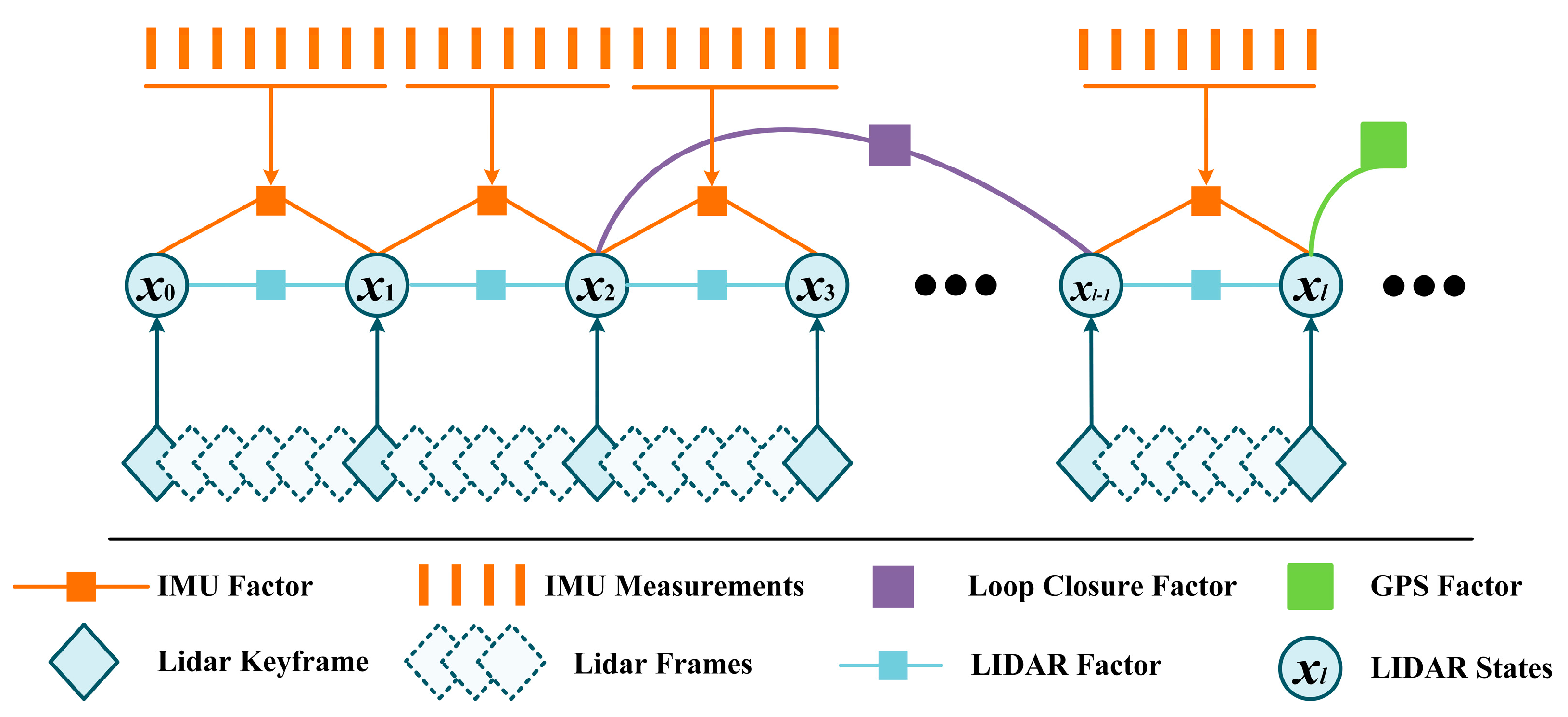
4.1. LIDAR-IMU Tightly Coupled System

On the theoretical basis of pre-integration, a large amount of LIO-related work has gradually emerged in recent years. One of the early approaches to tightly couple LIDAR and IMU was proposed in LIPS [55], which employs a graph-based optimization framework. In this framework, a planar representation of the closest point is proposed. A set of point clouds is parameterized as plane features, and then the residuals-function is converted into the differences between the plane parameters of two frames, which, together with the residual term of the IMU pre-integration, constitutes the final optimization function. This tightly coupled approach was deeply influenced by the VINS series and began to emerge in the field of LIDAR SLAM. This form lays a solid foundation for the subsequent LIO and LVI tightly coupled systems.
The pre-integration of the IMU was used for removing the distortion of the raw point cloud in Gentil’s work [56]. It tightly integrates the IMU and LIDAR data into a batch manifold optimization formulation, which describes the motion in the LIDAR scan based on the extrinsic parameters of IMU. The system also considers the first-order form of the pre-integration error to the time difference and solves the problem of hardware time asynchrony. Ye [57] proposed a tightly coupled LIDAR inertial localization and mapping framework, LIOM (LIO-mapping), which jointly optimizes measurements from LIDAR and IMU. A sliding-window model was further used to maintain a certain scale of optimization data. The accuracy of LIOM is better than that of LOAM. However, real-time cannot be achieved since LIOM is designed to process the measurements by all sensors.
Inspired by Hess’s work [58], Ding [59] introduced the subgraph representation of 2D SLAM into the 3D LIDAR odometry and added inertial data to establish motion prediction and constraints between frames. In this system, the 3D occupancy grid method is utilized to replace the 2D occupancy grid to realize the pose measurement of all 6 degrees of freedom. Finally, the iterative solution is performed in the solver Ceres [60]. The system innovatively joins the environmental change detection (ECD) module, which can detect whether the known surrounding environment has changed. However, this feature is not used to eliminate the influence of unknown dynamic environment on SLAM.
The authors of LeGO-LOAM released LIO’s follow-up work LIO-SAM [61] in combination with IMU-related theories. The system builds the LIDAR-inertial odometry on a factor graph, and multiple relative and absolute measurements including closed loops are incorporated into the system as factors, as shown in Figure 6. The innovation of LIO-SAM is to marginalize old pose and point cloud data to replace matching scans to global maps. The system uses local map matching instead of global matching to significantly improve real-time performance. In addition, the system also adds the GPS absolute positioning factor [62], which is used to correct the long-term drift of the system. However, since feature extraction relies on geometric environments, this method still cannot work for a long time in open scenes.
The latest work of LIRO [63] proposed a sensor fusion scheme combining LIO with UWB ranging. The solution can be easily deployed with minimal cost and time. The system tightly couples IMU, LIDAR, and UWB data with timestamp-based robot states in a sliding window to construct a cost function consisting of UWB, LO, and IMU pre-integrations. Finally, a factor graph model is used to incrementally marginalize and update the data within the window. However, the usage scenarios of UWB have great limitations. The system will no longer have an advantage in a huge range of occlusion scenarios.
The tightly coupled LIO system proposed by Chen [64] further refines the front-end. He proposed an efficient algorithm to simultaneously extract the explicit mixed features of the original point cloud, including ground features, edge features, and plane features. The system also introduced a deep learning-based LPD-Net to generate global descriptors for point clouds. The loop closures detection can be accomplished in the key frame database. This method greatly improves the accuracy of closed loop detection. In order to ensure the real-time performance of the system, Li [65] proposed a quantitative evaluation method for point cloud feature constraints and a screening algorithm for key features. An effective compromise is traded off between accuracy and computational cost. Lv [66] proposed a high-accuracy continuous-time trajectory estimation framework for LIO systems to efficiently fuse high-frequency asynchronous sensor data. The system uses a non-rigid body registration method for continuous-time trajectory estimation. Dynamic and static control points are defined to further optimize trajectory estimation. At the same time, a two-stage closed-loop correction method is proposed to effectively update the closed-loop pose and control points, respectively. However, the computational cost of closing the loop is not reported, nor does it address the uncertainty in motion that might suffer from motion degradation.
RF-LIO [67] is a dynamic SLAM framework proposed on the basis of LIO-SAM. The system adaptively adds a multi-resolution range image composed of point clouds and removes moving objects using tightly coupled LIDAR inertial odometry. The LIDAR scans are then matched with the subgraphs. Therefore, it can obtain accurate pose estimation results even in highly dynamic environments. LIO tightly coupled systems based on solid-state LIDAR have also been gradually attracting attention. However, LIO degradation still occurs when moving in open scenes for a long time. FAST-LIO [68] proposed an efficient and robust LIO framework based on tightly coupled iterative Kalman filters for UAV systems. However, the system discards the impact of historical data on the current state. Global pose correction cannot be performed.
The tight coupling of the inertial system will undoubtedly increase the computational burden of the system while improving the accuracy. Most of the existing algorithms improve computing speed by marginalizing historical data or limiting local map capacity. The back end optimization generally only builds the pose graph of the LIDAR without adding the bias and speed measured by the IMU. These methods achieve excellent results in most scenarios. However, due to the dependence on geometric features, once the inertial system loses the LO constraint in the open unstructured scene, the SLAM will suffer serious drift and degradation. The related work on the LIDAR-IMU tightly coupled system is compared in Table 4.
With the development and improvement of the IMU pre-integration theory, the LO system can establish a stronger constraint relationship with the IMU. The localization accuracy of the SLAM system has also been further improved. However, tight coupling involves a great amount of computation. Finding a balance between the speed and the precision is the difficulty of this stage of work.

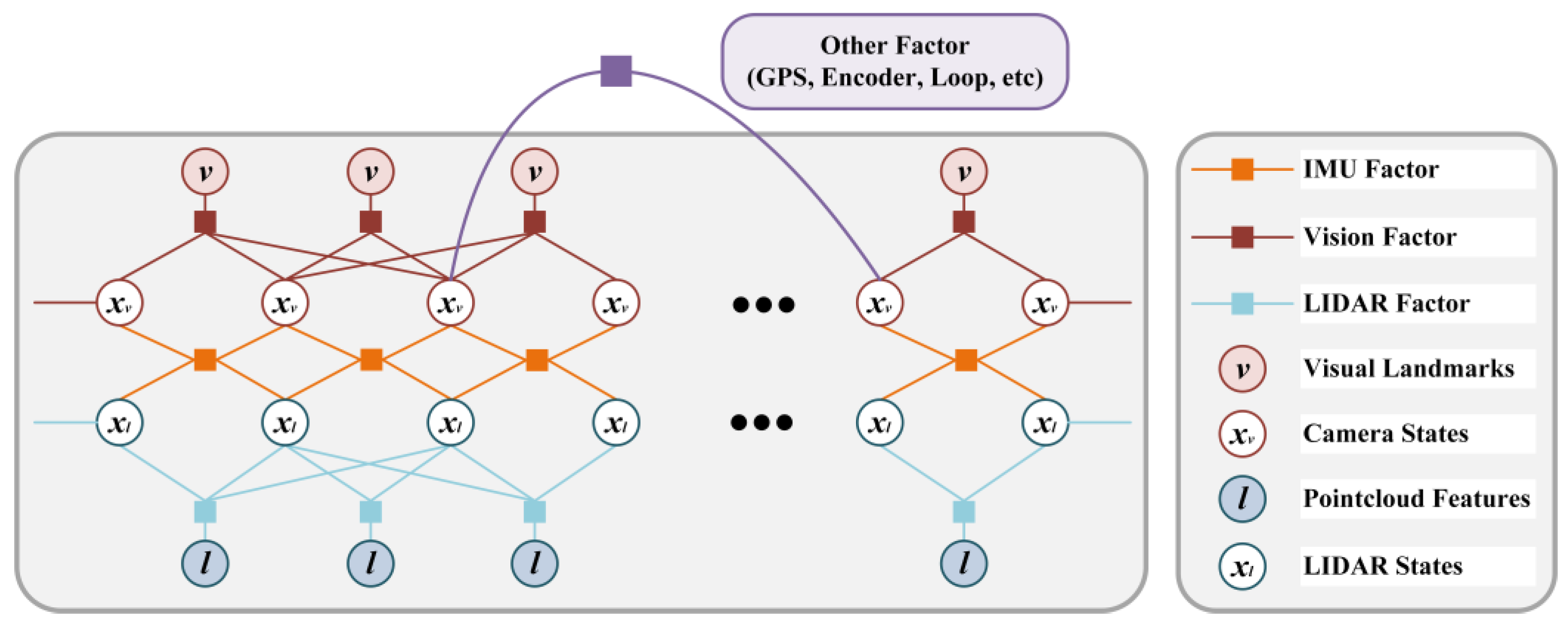
4.2. LIDAR-Visual-IMU Tightly Coupled System

Although the study of visual SLAM started relatively late, it quickly became a research hotspot of SLAM technology due to its advantages of small size and low cost. Many VIO works have reported in recent years. Vision forms an excellent complementation with LIDAR because it is not constrained by the structure of the scene. Therefore, LVI systems have received increasing attention owing to their stronger robustness in sensor degradation scenarios.
The strong data association between point clouds and images enables the system to tightly combine multiple effective features in the preprocessing stage. They will play an important role in the matching and optimization process. The LVI tightly coupled system is divided into two coupling methods based on optimization and filtering. The optimization-based approach tightly integrates the error models of individual sensors and reduces the sensitivity of time synchronization by using local maps or sliding windows. This method simultaneously optimizes historical poses and achieves real-time performance with BA. In addition, this paper classifies the tight association of sensor data level as a special category of the tightly coupled. Although no joint optimization is performed during the pose solving, these works strongly correlate the data through preprocessing, and already contain the necessary key information of the sensor in single objective function. They all have a closed system, which is less scalable and compatible with other sensors. Filter-based approaches merely use the sensor data of the current frame and rely on the time synchronization of each data. Since the influence of historical data on the current pose is not considered, the amount of computation is relatively small and the scalability is relatively good.
LIMO [69] is one of the multi-sensor fusion positioning systems. The system performs strong correlation between point clouds and images through a variety of data preprocessing methods to achieve a stable and robust system. The system performs foreground segmentation, plane fitting, and ground fitting on point clouds for different scenes so as to obtain the best depth estimation of visual features. The system combines the 3D-2D PNP (Perspective-n-Point-Problem) [70] pose estimation method and the 2D-2D epipolar constraint [71] to achieve a good localization effect. Reference [72] is another example of strong data correlation, where point and line features are extracted in the image, and the position information of points and lines are obtained by a similar method to LIMO. Furthermore, a 3D-3D ICP model and reprojection error functions of points and lines are constructed, which achieves higher accuracy pose estimation. Recent work [73] fuses data from two sensors in a higher-level space using geometric features co-detected in LIDAR scan and image data. Correspondences between 3D lines extracted in the LIDAR scan and 2D lines detected in the image were determined. Wang [74] proposed a DSP-SLAM system by combining object detection with SLAM. This work uses a DeepSDF network to generate object shape vectors and 7D poses from keyframed point cloud and image data. Sparse point clouds and image segmentation results are used as observations to minimize surface loss and depth rendering loss functions. Object reconstruction and pose update are added to the ORB-SLAM2-based BA factor graph to simultaneously optimize camera pose, map points, and object pose. These works do a lot of meaningful work on data association, which makes the whole system more robust. However, these systems obviously lack the tight coupling of the optimization process. The combination of correlation between raw data and integration of errors will lead to a stronger system.
On the other hand, the very matured framework of the LIO system paves the way for the establishment of the LVI tightly coupled system, which has led to the emergence of a large number of tightly coupled systems based on the optimized LIDAR-Vision-IMU in the past two years. GR-Fusion [75] uses camera, IMU, LIDAR, GNSS, and encoder of motion chassis as main sensors to build a factor graph model in a sliding window. The LIDAR factor, the visual factor, the IMU factor, and the odometry factor are added as primary constraints to the factor graph. Meanwhile, local constraints are tightly coupled with GNSS constraints to optimize the global state of the robot. The system can detect the degradation of the sensor in real time and flexibly configure multi-working modes, which is suitable for a wide range of scenarios. LVIO-Fusion [76] adopts a similar system architecture. The difference is that the binocular camera is used as the visual sensor. This paper innovatively proposed different optimization strategies for straight and turning. Moreover, reinforcement learning networks are introduced to adaptively adjust the weights of sensors in different scenarios. LVI-SAM [77] is the latest work by the authors of LeGO-LOAM and LIO-SAM. The system consists of VIS (Visual-Inertial System) and LIS (LIDAR-Inertial System). VIS can provide pose prior for LIS, which can provide pose estimation and accurate feature point depth for VIS initialization. However, this system does not consider the marginalization of the LIO system and the problem of timestamp synchronization.
Some recent odometry systems also employ a tightly coupled approach to obtain low-drift pose estimates. Super Odometry [78] and MetroLoc [79] both use an LVI system with an IMU as the main sensors. The system consists of three parts: IMU odometer, VIO, and LIO. The observation data provided by VIO and LIO can constrain the bias of the IMU. On the other hand, the constrained IMU odometry provides predictions for VIO and LIO to achieve coarse-to-fine pose estimation, which is shown in Figure 7. The system can simultaneously extend GPS and wheel odometer with robustness to sensor degradation. Wisth [80] proposed a tightly coupled system based on LIDAR and a binocular camera. The factor graph optimization problem is composed of initial prior factor, visual factor, line factor, plane factor, and IMU pre-integration, and is solved by GTSAM [81]. The system shares a representation of vision-based point features and point cloud-based line and area features. The reprojection error function is then defined by parameterizing different features. In addition, based on the data timestamp of the camera, the system splits and merges the adjacent scan data of LIDAR to realize the time hard synchronization at the software level. There is no doubt that these works have good real-time positioning effect. However, a pure odometer system often discards historical data and only focuses on current or local observations, which leads to the loss of correlation and optimization of global data. Therefore, excellent front end odometer and reasonable back end optimization are necessary for SLAM system.
Filter-based methods also play an important role in the field of multi-sensor fusion. For joint state optimization, many methods use the EKF or the MSCKF framework [82]. Yang [83] used MSCKF to tightly couple planar features from RGB-D sensors, IMU measurements, and visual point features within 3.5 m. To limit the scale of the state vector, the system linearly marginalizes most of the point features and retains a few point features with plane-enhanced constraints in the state vector as SLAM features. The LIC-Fusion proposed by Zuo [84] adopts the MSCKF fusion framework, which tightly combines IMU measurements, extracted LIDAR edge features, and sparse visual features. Subsequently, in the latest follow-up work, LIC-Fusion 2.0 [85], the authors introduced a sliding-window-based planar feature tracking method to efficiently process 3D LIDAR point clouds in real time. R2LIVE [86] is a tightly coupled work based on solid-state LIDAR. The system combines an error-state-based iterative Kalman filtering front end and a new step of factor graph optimization-based sliding window optimization to refine the visual pose and landmark estimation. It achieves high accuracy and robustness in harsh scenarios such as indoors, outdoors, tunnels, and high-speed motion. These methods are fast and computationally inexpensive, but are sensitive to time synchronization. Measurements during filtering may degrade or fail. Therefore, a special sorting mechanism is required to guarantee the correct order of the measurement results of the different sensors.
In this paper, the LVI tightly coupled system is divided into three parts: strong data correlation, nonlinear optimization tight coupling, and state filter. Among them, the tightly coupled front end based on optimization is the main implementation. Table 5 compares the related works of the LIDAR-Vision-IMU tightly coupled system.
The emergence of a complete system in which LIDAR, vision, and IMU cooperate and complement each other is a milestone for multi-sensor fusion SLAM. The integration is not limited to these three sensors. Wheel/leg odometer and GNSS have also been effectively integrated into the system. Similarly, the increase in computational complexity is one of the toughest problems. In addition, there are some details that need to be optimized, such as dynamic environments, unstructured environments, rain and snow weather.

5. Performance Evaluation
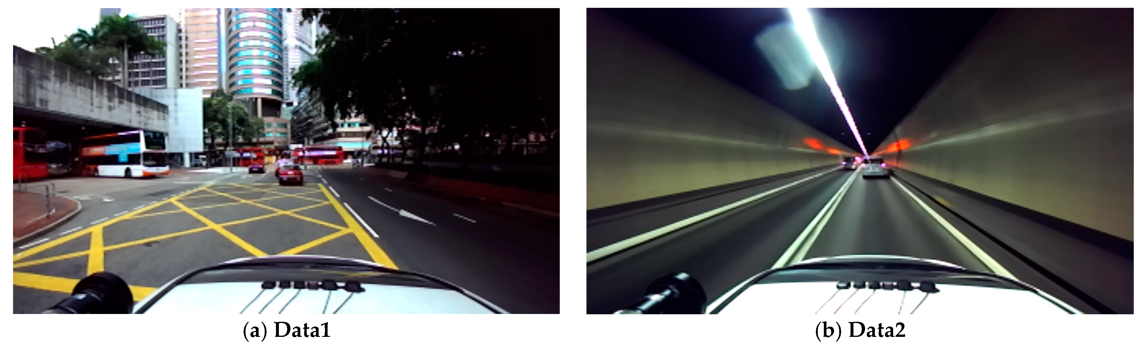
5.1. SLAM Datasets

Evaluating the performance of SLAM algorithms is often inseparable from the help of open-source datasets. The mobile carriers for research and application of 3D LIDAR SLAM include unmanned vehicles, unmanned ships, and unmanned aerial vehicles. However, the current LIDAR point cloud datasets are mainly for autonomous driving scenarios. Data collection in outdoor scenes is complex and cumbersome, involving time synchronization, coordinate calibration, and calibration among various sensors. Public datasets save the time for data preparation for algorithmic research. The sequences and benchmarking frameworks provided also facilitate algorithm development.
The current public LIDAR-based datasets in the field include: KITTI dataset [87], which is currently the largest international evaluation dataset for autonomous driving scenarios and is also the most commonly used dataset in academia. The Waymo dataset [88] is a data-open project of the autonomous driving company Waymo. The PandaSet dataset [89] is used to develop safe and controllable autonomous driving technology in complex environments and extreme weathers. Oxford Robotcar dataset [90] is a public dataset proposed by Oxford University Robotics Laboratory. The UrbanNav dataset [91] provides a challenging data source to the community to further accelerate the study of accurate and robust positioning in challenging urban canyons. The UrbanNav dataset includes complex and dynamic urban road environments and closed tunnel environments. It also provides the real pose of the GNSS system as a reference. Compared with the commonly used KITTI dataset, the collection environment of the UrbanNav dataset is closer to the complex environment of unmanned driving. At the same time, the related team of the UrbanNav dataset provides an overview [92] of LIDAR Odometry, which uses this dataset to evaluate open-source algorithms based on point clouds and features, respectively.
Obviously, the complex scene of the city can magnify the advantages and disadvantages of the SLAM algorithm. Therefore, this paper uses the UrbanNav dataset to evaluate some open-source algorithms in the following section.

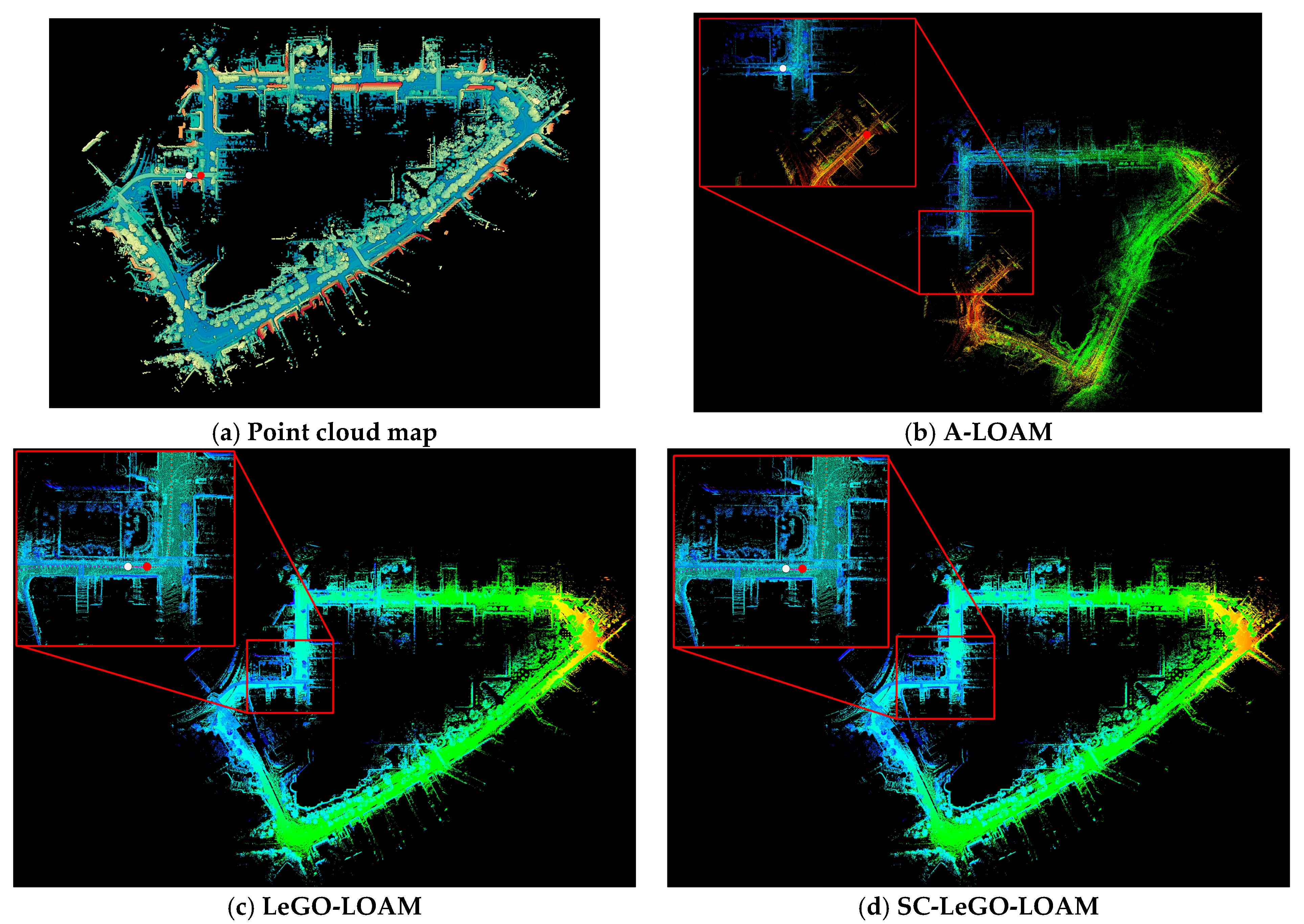
5.2. Performance Comparison

The evaluation of the SLAM algorithm is mainly based on evaluating the positioning accuracy. The relative pose error (RPE) is used to describe the accuracy of the pose difference between two frames separated by a certain time difference. The changes of the real pose and the estimated pose are calculated at the same time interval. Then, the difference between the two is calculated to obtain the relative pose error. Afterwards, the relative pose error of each period of time can be counted by the root mean square error (RMSE) to obtain the overall value. The absolute trajectory error (ATE) describes the direct difference between the estimated pose and the real pose, which can intuitively reflect the accuracy of the algorithm and the global consistency of the trajectory. Many SLAM algorithms and review papers have analyzed the performance of open-source algorithms using datasets in the experimental part. Jonnavithula [93] provides an overview of existing LO systems for the application environment of autonomous driving. This paper uses the KITTI dataset to experimentally verify some of the reviewed algorithms. Huang [92] uses the UrbanNav dataset for comparison to demonstrate the pros and cons of point cloud-based and feature-based localization methods. Yokozuka [18] also conducted many comparative experiments using the KITTI dataset in the experimental part of his algorithm.
This paper selects five open-source 3D LIDAR SLAM algorithms for testing and evaluation. They are A-LOAM [94], LeGO-LOAM [12], SC-LeGO-LOAM [24], LIO-SAM [61], and F-LOAM [95]. A-LOAM is an open-source version that uses an optimizer for code simplification based on LOAM. SC-LeGO-LOAM uses scan context to optimize loop closure detection based on LeGO-LOAM. F-LOAM is an odometer system that only relies on LIDAR but has good performance. We apply them to ROS running on a laptop with an Intle i7-10875H CPU to achieve the functionality, and the platform has 2 × 8 GB of RAM memory and an RTX2060 GPU. All algorithms are evaluated and compared in experiments based on the UrbanNav public dataset benchmark. We collect experimental results under the same conditions and carry out performance metrics in order to evaluate the performance of the tested algorithms. This paper focuses on two competitive datasets, UrbanNav-HK-Medium-Urban-1 (Data1) and UrbanNav-HK-Tunnel-1 (Data2). Data1 are in an urban center area with heavy traffic and towering buildings. Data2 were collected while moving fast in a closed tunnel. The pictures corresponding to the two scenarios are shown in Figure 8.
First, we focus on the mapping effects of the five algorithms. Mapping is based on positioning, which can intuitively show the overall operation effect of SLAM. We take Data1 as an example to show the official environment map and the different results of each algorithm (as shown in Figure 9).
The comparison chart intuitively shows the mapping results of the five algorithms. A-LOAM suffers severe drift in traffic-congested sections, which leads to poor localization and mapping. The mappings of LeGO-LOAM, SC-LeGO-LOAM, and LIO-SAM are good and the localizations are effectively constrained by the closed loop. However, it is worth emphasizing that the search radius of the closed loop detection of LeGO-LOAM and LIO-SAM is adjusted to 50 m before the closed loop can be accurately identified. F-LOAM still has high global consistency in the absence of loop closure detection.
Second, trajectories of different algorithms and ground truth are plotted together for comparison (as shown in Figure 10). In order to facilitate the observation, we take the trajectory generated by the first lap of data for comparison. The first loop closure occurs at the zoomed-in position on the left, which is the same as that marked in the point cloud map.
The trajectories generated by the five algorithms are clearly shown in Figure 10. The trajectory of A-LOAM has poor positioning accuracy when there are many traffic jams or dynamic vehicles. Therefore, it basically loses the positioning ability in the urban canyon environment. The other four algorithms have good global consistency. It is worth emphasizing that F-LOAM only deviates a small distance from the closed loop position without loop closure detection. The positioning accuracies of the five algorithms are listed in Table 6. We use the RMSE and mean of relative pose errors to describe the accuracy of the algorithm. The odometer’s average processing time for per-frame (APTFP) is used to describe the algorithm efficiency.
From the data in the table, it can be seen that the overall performances of F-LOAM and LIO-SAM are better. The relative translation error of F-LOAM is the smallest, while the relative rotational error of LIO-SAM is the smallest. The addition of IMU pre-integration can effectively improve the positioning accuracy of rotation. The positioning accuracy and processing time of A-LOAM are relatively poor. We recommend using LIO-SAM when there is a closed loop in the environment dealt with. If no closed loop presents, the real-time performance of F-LOAM is better.
Finally, the operation on Data2 will be summarized and discussed. The tunnel environment in Data2 is more challenging than congested urban canyons. There are very few structural features and the light changes rapidly in the closed tunnel. The tunnel seems to be a long corridor so that the point cloud data generated by LIDAR is basically the same no matter where it is located. Unfortunately, none of the five algorithms can effectively complete the positioning process without using GPS data. However, they show different behaviors and have different odometer failure locations. The real point cloud map and the actual performance of the five algorithms are shown in Figure 11.
The A-LOAM was disabled before entering the tunnel due to the large number of dynamic vehicles congested around the LIDAR. The results of LeGO-LOAM and SC-LeGO-LOAM are similar. They both degenerate when they first enter the tunnel because their system compositions are basically the same. F-LOAM performs slightly better than the previous two thanks to the feature weights it assigns. Degradation of F-LOAM occurs after a certain distance in the tunnel. Finally, LIO-SAM performs the best. The front end of LIO-SAM is also feature-based. However, the system can still run robustly for some time as the LO degenerates due to the addition of IMU data constraints. This allows it to travel the longest distance effectively in the tunnel. Obviously, the tight coupling of the IMU cannot completely solve the long-distance tunneling problem.
The long corridor problem is a difficult problem often faced in practical applications. The above experiments show that assigning weights to features and adding IMU pre-integration can effectively alleviate the phenomenon of odometer degradation. Clearly, feature-based methods encounter a bottleneck in the tunnel environment. This problem will be better solved if the precise control model and kinematic model of the robot chassis are combined with a feature-based odometry system or aided by visual features [96]. At the same time, UWB is also suitable for such closed scenes within a certain range. This is also an effective way of carrying out multi-sensor fusion.

6. Conclusions and Future Outlook

The development of SLAM technology based on 3D LIDAR in recent years has been rapid. Among them, excellent works of multi-sensor fusion have emerged in an endless stream. Throughout the development history of fusion SLAM, we have seen from filter-based probabilistic methods to information-based optimization methods; from raw data-assisted front end fusion to error-coupling-based back end optimization; from single sensor systems to complex systems with multiple subsystems coupled; from independent error models to tightly coupled complete graphical models. Various application scenarios and demands have promoted the diversity of SLAM technology. Continuous advancements in sensor technology provide the foundation and impetus for it.
This paper mainly classifies and summarizes the papers and works that have appeared in recent years based on the data coupling method of the SLAM system. The main innovations of the paper are mentioned together when describing the details of data association. The strengths and weaknesses of each work are based on the qualitative analysis of the system composition. However, our work is far from perfect. Obviously, this paper does not list all related works for readers’ reference. Only a portion of representative works are shown. There are more works based on deep learning for multi-sensor fusions, mostly used in environment perception, object detection and semantic segmentation. They may play auxiliary roles in SLAM systems.
Multi-sensor fusion is a key to building robust systems. Complex systems based on multi-sensors need to be lightweight, accurate, scalable, and versatile for SLAM. From the experimental part, we know that dynamic environment, object occlusion, and long corridor environment are the key challenges for feature-based SLAM methods. Combining the sensor with the control model of the robot or vehicle can effectively alleviate the problem of odometer degradation in special cases. With the increase of the number of sensors, the amount of data, and the continuous expansion of application scenarios, it is difficult for SLAM systems to further improve the accuracy of positioning and mapping within a specified computing time. Therefore, SLAM has large development space in the applications of various scenes. Distributed multi-robot collaboration, land–air collaboration, and sea–air collaboration systems can effectively solve the problems faced in large scenes. In addition, hardware acceleration and parallel processing feature extraction and pose optimization can effectively relieve the computational pressure of the system due to the multi-sensor data fusion. On the other hand, deep learning is undoubtedly one of the hottest directions at present. There have been a lot of efforts towards combining deep learning with SLAM systems. The application of deep learning can be seen in almost all key steps such as feature extraction, depth estimation, environment perception, pose estimation, and semantic map. In the current works, deep learning only replaced limited parts of the SLAM system. For example, optimizing depth estimation of monocular camera to obtain landmark points, directly estimating pose without feature extraction, perceiving the environment to distinguish moving objects, and building high-precision semantic maps. These are research directions with great potential in the future. The application of deep learning will further improve and expand the performance and functions of SLAM. In future work, the combination of data fusion of multiple sensors and deep learning to optimize and improve the SLAM algorithm will receive more attention.

Author Contributions

Collection and organization of references, C.C. and W.W.; summarization and classification of references, X.X and L.Z.; writing—original draft preparation, L.Z.; writing—review and editing, L.Z., X.X. and J.Y.; supervision, Y.R., Z.T. and M.L. All authors have read and agreed to the published version of the manuscript.

Funding

This research was funded by Changzhou Sci&Tech Program (Grant No. CE20215041), the Fundamental Research Funds for the Central Universities (Grant No. B220202023), and Jiangsu Key R&D Program (Grant No. BE2020082-1).

Data Availability Statement

Not applicable.

Conflicts of Interest

The authors declare no conflict of interest.

References

  1. Montemerlo, M.; Becker, J.; Bhat, S.; Dahlkamp, H.; Dolgov, D.; Ettinger, S.; Haehnel, D.; Hilden, T.; Hoffmann, G.; Huhnke, B.; et al. Junior: The Stanford Entry in the Urban Challenge. J. Field Robot. 2008, 25, 569–597. [Google Scholar] [CrossRef] [Green Version]
  2. Levinson, J.; Askeland, J.; Becker, J.; Dolson, J.; Held, D.; Kammel, S.; Kolter, J.Z.; Langer, D.; Pink, O.; Pratt, V.; et al. Towards Fully Autonomous Driving: Systems and Algorithms. In Proceedings of the 2011 IEEE Intelligent Vehicles Symposium (IV), Baden-Baden, Germany, 5–9 June 2011; pp. 163–168. [Google Scholar]
  3. He, X.; Gao, W.; Sheng, C.Z.; Zhang, Z.T.; Pan, S.G.; Duan, L.J.; Zhang, H.; Lu, X.Y. LiDAR-Visual-Inertial Odometry Based on Optimized Visual Point-Line Features. Remote Sens. 2022, 14, 662. [Google Scholar] [CrossRef]
  4. Tee, Y.K.; Han, Y.C. Lidar-Based 2D SLAM for Mobile Robot in an Indoor Environment: A Review. In Proceedings of the 2021 International Conference on Green Energy, Computing and Sustainable Technology (GECOST), Miri, Malaysia, 7–9 July 2021; pp. 1–7. [Google Scholar]
  5. Bresson, G.; Alsayed, Z.; Yu, L.; Glaser, S. Simultaneous Localization and Mapping: A Survey of Current Trends in Autonomous Driving. IEEE Trans. Intell. Vehic. 2017, 2, 194–220. [Google Scholar] [CrossRef] [Green Version]
  6. Cadena, C.; Carlone, L.; Carrillo, H.; Latif, Y.; Scaramuzza, D.; Neira, J.; Reid, I.; Leonard, J.J. Past, Present, and Future of Simultaneous Localization and Mapping: Toward the Robust-Perception Age. IEEE Trans. Robot. 2016, 32, 1309–1332. [Google Scholar] [CrossRef] [Green Version]
  7. Debeunne, C.; Vivet, D. A Review of Visual-LiDAR Fusion Based Simultaneous Localization and Mapping. Sensors 2020, 20, 2068. [Google Scholar] [CrossRef] [PubMed] [Green Version]
  8. Taheri, H.; Xia, Z.C. SLAM; Definition and Evolution. Eng. Appl. Artif. Intell. 2021, 97, 104032. [Google Scholar] [CrossRef]
  9. Zhiguo, Z.; Jiangwei, C.; Shunfan, D. Overview of 3D Lidar SLAM Algorithms. Chin. J. Sci. Instrum. 2021, 42, 13–27. [Google Scholar]
  10. Leonard, J.J.; Durrant-Whyte, H.F. Directed Sonar Sensing for Mobile Robot. Navigation; Kluwer Academic Publishers: Norwood, MA, USA, 1992. [Google Scholar]
  11. Ji, Z.; Singh, S. LOAM: Lidar Odometry and Mapping in Real-Time. In Proceedings of the Robotics: Science and Systems Conference (RSS), Berkeley, CA, USA, 12–14 July 2014. [Google Scholar]
  12. Shan, T.; Englot, B. LeGO-LOAM: Lightweight and Ground-Optimized Lidar Odometry and Mapping on Variable Terrain. In Proceedings of the 2018 IEEE/RSJ International Conference on Intelligent Robots and Systems (IROS), Madrid, Spain, 1–5 October 2018; pp. 4758–4765. [Google Scholar]
  13. Zermas, D.; Izzat, I.; Papanikolopoulos, N. Fast Segmentation of 3D Point Clouds: A Paradigm on LiDAR Data for Autonomous Vehicle Applications. In Proceedings of the 2017 IEEE International Conference on Robotics and Automation (ICRA), Singapore, 29 May–3 June 2017; pp. 5067–5073. [Google Scholar]
  14. Huo, X.; Dou, L.; Lu, H.; Tian, B.; Du, M. A Line/Plane Feature-Based Lidar Inertial Odometry and Mapping. In Proceedings of the 2019 Chinese Control Conference (CCC), Guangzhou, China, 27–30 July 2019; pp. 4377–4382. [Google Scholar]
  15. Zhang, S.; Xiao, L.; Nie, Y.; Dai, B.; Hu, C. Lidar Odometry and Mapping Based on Two-Stage Feature Extraction. In Proceedings of the 2020 39th Chinese Control Conference (CCC), Shenyang, China, 27–29 July 2020; pp. 3966–3971. [Google Scholar]
  16. Gonzalez, C.; Adams, M. An Improved Feature Extractor for the Lidar Odometry and Mapping (LOAM) Algorithm. In Proceedings of the 2019 International Conference on Control, Automation and Information Sciences (ICCAIS), Chengdu, China, 23–26 October 2019; pp. 1–7. [Google Scholar]
  17. Lee, S.-W.; Hsu, C.-M.; Lee, M.-C.; Fu, Y.-T.; Atas, F.; Tsai, A. Fast Point Cloud Feature Extraction for Real-Time SLAM. In Proceedings of the 2019 International Automatic Control Conference (CACS), Keelung, Taiwan, 13–16 November 2019; pp. 1–6. [Google Scholar]
  18. Yokozuka, M.; Koide, K.; Oishi, S.; Banno, A. LiTAMIN2: Ultra Light LiDAR-Based SLAM Using Geometric Approximation Applied with KL-Divergence. In Proceedings of the 2021 IEEE International Conference on Robotics and Automation (ICRA), Xi’an, China, 30 May–5 June 2021; pp. 11619–11625. [Google Scholar]
  19. Behley, J.; Stachniss, C. Efficient Surfel-Based SLAM Using 3D Laser Range Data in Urban Environments. In Proceedings of the 14th Conference on Robotics-Science and Systems (RSS), Pittsburgh, PA, USA, 26–30 June 2018. [Google Scholar]
  20. Park, C.; Moghadam, P.; Kim, S.; Elfes, A.; Fookes, C.; Sridharan, S. Elastic LiDAR Fusion: Dense Map-Centric Continuous-Time SLAM. In Proceedings of the 2018 IEEE International Conference on Robotics and Automation (ICRA), Brisbane, QLD, Australia, 21–25 May 2018; pp. 1206–1213. [Google Scholar]
  21. Droeschel, D.; Behnke, S. Efficient Continuous-Time SLAM for 3D Lidar-Based Online Mapping. In Proceedings of the 2018 IEEE International Conference on Robotics and Automation (ICRA), Brisbane, QLD, Australia, 21–25 May 2018; pp. 5000–5007. [Google Scholar]
  22. Pfister, H.; Zwicker, M.; van Baar, J.; Gross, M. Surfels: Surface Elements as Rendering Primitives. In Proceedings of the Computer Graphics Annual Conference, New Orleans, LA, USA, 23–28 July 2000; pp. 335–342. [Google Scholar]
  23. Pan, Y.; Xiao, P.C.A.; He, Y.J.; Shao, Z.L.; Li, Z.S. MULLS: Versatile LiDAR SLAM via Multi-Metric Linear Least Square. In Proceedings of the 2021 IEEE International Conference on Robotics and Automation (ICRA), Xi’an, China, 30 May–5 June 2021; pp. 11633–11640. [Google Scholar]
  24. Kim, G.; Kim, A.; Kosecka, J. Scan Context: Egocentric Spatial Descriptor for Place Recognition within 3D Point Cloud Map. In Proceedings of the 2018 IEEE/RSJ International Conference on Intelligent Robots and Systems (IROS), Madrid, Spain, 1–5 October 2018; pp. 4802–4809. [Google Scholar]
  25. Wang, H.; Wang, C.; Xie, L.H. Intensity Scan Context: Coding Intensity and Geometry Relations for Loop Closure Detection. In Proceedings of the 2020 IEEE International Conference on Robotics and Automation (ICRA), Paris, France, 31 May–31 August 2020; pp. 2095–2101. [Google Scholar]
  26. Lin, J.; Zhang, F. A Fast, Complete, Point Cloud Based Loop Closure for LiDAR Odometry and Mapping. arXiv 2019. [Google Scholar] [CrossRef]
  27. Lin, J.; Zhang, F. Loam Livox: A Fast, Robust, High-Precision LiDAR Odometry and Mapping Package for LiDARs of Small FoV. In Proceedings of the 2020 IEEE International Conference on Robotics and Automation (ICRA), Paris, France, 31 May–31 August 2020; pp. 3126–3131. [Google Scholar]
  28. Zhang, J.; Singh, S. Visual-Lidar Odometry and Mapping: Low-Drift, Robust, and Fast. In Proceedings of the 2015 IEEE International Conference on Robotics and Automation (ICRA), Seattle, WA, USA, 26–30 May 2015; pp. 2174–2181. [Google Scholar]
  29. Zhang, J.; Singh, S. Laser-Visual-Inertial Odometry and Mapping with High Robustness and Low Drift. J. Field Robot. 2018, 35, 1242–1264. [Google Scholar] [CrossRef]
  30. Caselitz, T.; Steder, B.; Ruhnke, M.; Burgard, W. Monocular Camera Localization in 3D LiDAR Maps. In Proceedings of the 2016 IEEE/RSJ International Conference on Intelligent Robots and Systems (IROS), Daejeon, Korea, 9–14 October 2016; pp. 1926–1931. [Google Scholar]
  31. Zhang, L.; Xu, X.; Cao, C.; He, J.; Ran, Y.; Tan, Z.; Luo, M. Robot Pose Estimation Method Based on Image and Point Cloud Fusion with Dynamic Feature Elimination. Chin. J. Lasers 2022, 49, 0610001. [Google Scholar]
  32. Qin, T.; Li, P.; Shen, S. VINS-Mono: A Robust and Versatile Monocular Visual-Inertial State Estimator. IEEE Trans. Robot. 2018, 34, 1004–1020. [Google Scholar] [CrossRef] [Green Version]
  33. Zhang, M.; Han, S.; Wang, S.; Liu, X.; Hu, M.; Zhao, J. Stereo Visual Inertial Mapping Algorithm for Autonomous Mobile Robot. In Proceedings of the 2020 3rd International Conference on Intelligent Robotic and Control Engineering (IRCE), Oxford, UK, 10–12 August 2020; pp. 97–104. [Google Scholar]
  34. Qin, T.; Cao, S.; Pan, J.; Shen, S. A General Optimization-Based Framework for Global Pose Estimation with Multiple Sensors. arXiv 2019. [Google Scholar] [CrossRef]
  35. Wang, Z.; Zhang, J.; Chen, S. Robust High Accuracy Visual-Inertial-Laser SLAM System. In Proceedings of the 2019 IEEE/RSJ International Conference on Intelligent Robots and Systems (IROS), Macau, China, 4–8 November 2019; pp. 6636–6641. [Google Scholar]
  36. Shao, W.; Vijayarangan, S.; Li, C.; Kantor, G. Stereo Visual Inertial LiDAR Simultaneous Localization and Mapping. In Proceedings of the 2019 IEEE/RSJ International Conference on Intelligent Robots and Systems (IROS), Macau, China, 4–8 November 2019; pp. 370–377. [Google Scholar]
  37. Kaess, M.; Ranganathan, A.; Dellaert, F. iSAM: Incremental Smoothing and Mapping. IEEE Trans. Robot. 2008, 24, 1365–1378. [Google Scholar] [CrossRef]
  38. Kaess, M.; Johannsson, H.; Roberts, R. iSAM2: Incremental Smoothing and Mapping with Fluid Relinearization and Incremental Variable Reordering. In Proceedings of the 2011 IEEE International Conference on Robotics and Automation (ICRA), Shanghai, China, 9–13 May 2011; pp. 3281–3288. [Google Scholar]
  39. Khattak, S.; Nguyen, H.D.; Mascarich, F. Complementary Multi-Modal Sensor Fusion for Resilient Robot Pose Estimation in Subterranean Environments. In Proceedings of the 2020 International Conference on Unmanned Aircraft Systems (ICUAS), Athens, Greece, 1–4 September 2020; pp. 1024–1029. [Google Scholar]
  40. Camurri, M.; Ramezani, M.; Nobili, S.; Fallon, M. Pronto: A Multi-Sensor State Estimator for Legged Robots in Real-World Scenarios. Front. Robot. AI 2020, 7, 18. [Google Scholar] [CrossRef] [PubMed]
  41. Lowe, T.; Kim, S.; Cox, M. Complementary Perception for Handheld SLAM. IEEE Robot. Autom. Lett. 2018, 3, 1104–1111. [Google Scholar] [CrossRef]
  42. Zhu, Y.; Zheng, C.; Yuan, C. CamVox: A Low-cost and Accurate Lidar-assisted Visual SLAM System. In Proceedings of the 2021 IEEE International Conference on Robotics and Automation (ICRA), Xi’an, China, 30 May–5 June 2021; pp. 5049–5055. [Google Scholar]
  43. Mur-Artal, R.; Tardós, J.D. ORB-SLAM2: An Open-Source SLAM System for Monocular, Stereo, and RGB-D Cameras. IEEE Trans. Robot. 2017, 33, 1255–1262. [Google Scholar] [CrossRef] [Green Version]
  44. Shin, Y.; Park, Y.; Kim, A. Direct Visual SLAM Using Sparse Depth for Camera-LiDAR System. In Proceedings of the 2018 IEEE International Conference on Robotics and Automation (ICRA), Brisbane, QLD, Australia, 21–25 May 2018; pp. 5144–5151. [Google Scholar]
  45. Engel, J.; Koltun, V.; Cremers, D. Direct Sparse Odometry. IEEE Trans. Pattern Anal. Mach. Intell. 2016, 40, 611–625. [Google Scholar] [CrossRef]
  46. Reinke, A.; Chen, X.; Stachniss, C. Simple but Effective Redundant Odometry for Autonomous Vehicles. In Proceedings of the 2021 IEEE International Conference on Robotics and Automation (ICRA), Xi’an, China, 30 May–5 June 2021; pp. 9631–9637. [Google Scholar]
  47. Segal, A.; Hhnel, D.; Thrun, S. Generalized-ICP. In Proceedings of the Robotics: Science and Systems V (RSS), Seattle, WA, USA, 28 June–1 July 2009. [Google Scholar]
  48. Rusinkiewicz, S.; Levoy, M. Efficient variants of the ICP algorithm. In Proceedings of the Proceedings Third International Conference on 3-D Digital Imaging and Modeling, Quebec, QC, Canada, 28 May–1 June 2001; pp. 145–152. [Google Scholar]
  49. Biber, P.; Strasser, W. The normal distributions transform: A new approach to laser scan matching. In Proceedings of the Proceedings 2003 IEEE/RSJ International Conference on Intelligent Robots and Systems (IROS), Las Vegas, NV, USA, 27–31 October 2003; pp. 2743–2748. [Google Scholar]
  50. Park, J.; Zhou, Q.Y.; Koltun, V. Colored Point Cloud Registration Revisited. In Proceedings of the 2017 IEEE International Conference on Computer Vision (ICCV), Venice, Italy, 22–29 October 2017; pp. 143–152. [Google Scholar]
  51. Huang, K.; Stachniss, C. Joint ego-motion estimation using a laser scanner and a monocular Camera through relative orientation estimation and 1-DoF ICP. In Proceedings of the 2018 IEEE/RSJ International Conference on Intelligent Robots and Systems (IROS), Madrid, Spain, 1–5 October 2018; pp. 671–677. [Google Scholar]
  52. Wang, P.; Fang, Z.; Zhao, S. Vanishing Point Aided LiDAR-Visual-Inertial Estimator. In Proceedings of the 2021 IEEE International Conference on Robotics and Automation (ICRA), Xi’an, China, 30 May–5 June 2021; pp. 13120–13126. [Google Scholar]
  53. Forster, C.; Carlone, L.; Dellaert, F.; Scaramuzza, D. IMU Preintegration on Manifold for Efficient Visual-Inertial Maximum-a-Posteriori Estimation. In Proceedings of the 2015 Robotics Science and Systems (RSS), Rome, Italy, 17 July 2015. [Google Scholar]
  54. Forster, C.; Carlone, L.; Dellaert, F. On-Manifold Preintegration for Real-Time Visual--Inertial Odometry. IEEE Trans. Robot. 2017, 33, 1–21. [Google Scholar] [CrossRef] [Green Version]
  55. Geneva, P.; Eckenhoff, K.; Yang, Y. LIPS: LiDAR-Inertial 3D Plane SLAM. In Proceedings of the 2018 IEEE/RSJ International Conference on Intelligent Robots and Systems (IROS), Madrid, Spain, 1–5 October 2018; pp. 123–130. [Google Scholar]
  56. Gentil, C.L.; Vidal-Calleja, T.; Huang, S. IN2LAMA: INertial Lidar Localisation And Mapping. In Proceedings of the 2019 International Conference on Robotics and Automation (ICRA), Montreal, QC, Canada, 20–24 May 2019; pp. 6388–6394. [Google Scholar]
  57. Ye, H.; Chen, Y.; Liu, M. Tightly Coupled 3D Lidar Inertial Odometry and Mapping. In Proceedings of the 2019 International Conference on Robotics and Automation (ICRA), Montreal, QC, Canada, 20–24 May 2019; pp. 3144–3150. [Google Scholar]
  58. Hess, W.; Kohler, D.; Rapp, H. Real-time loop closure in 2D LIDAR SLAM. In Proceedings of the 2016 IEEE International Conference on Robotics and Automation (ICRA), Stockholm, Sweden, 16–21 May 2016; pp. 4322–4328. [Google Scholar]
  59. Ding, W.; Hou, S.; Gao, H. LiDAR Inertial Odometry Aided Robust LiDAR Localization System in Changing City Scenes. In Proceedings of the 2020 IEEE International Conference on Robotics and Automation (ICRA), Paris, France, 31 May–31 August 2020; pp. 1271–1278. [Google Scholar]
  60. Ceres Solver. Available online: http://ceres-solver.org (accessed on 4 May 2022).
  61. Shan, T.; Englot, B.; Meyers, D.; Wang, W.; Ratti, C.; Rus, D. LIO-SAM: Tightly-Coupled Lidar Inertial Odometry via Smoothing and Mapping. In Proceedings of the 2020 IEEE/RSJ International Conference on Intelligent Robots and Systems (IROS), Las Vegas, NV, USA, 24 October–24 January 2021; pp. 5135–5142. [Google Scholar]
  62. Moore, T.; Stouch, D. A Generalized Extended Kalman Filter Implementation for the Robot Operating System. In Proceedings of the 13th International Conference on Intelligent Autonomous Systems (IAS), Padova, Italy, 15–18 July 2016; pp. 335–348. [Google Scholar]
  63. Nguyen, T.-M.; Cao, M.; Yuan, S.; Lyu, Y.; Nguyen, T.H.; Xie, L. LIRO: Tightly Coupled Lidar-Inertia-Ranging Odometry. In Proceedings of the 2021 IEEE International Conference on Robotics and Automation (ICRA), Xi’an, China, 30 May–5 June 2021; pp. 14484–14490. [Google Scholar]
  64. Chen, W.; Zhao, H.; Shen, Q.; Xiong, C.; Zhou, S.; Liu, Y.-H. Inertial Aided 3D LiDAR SLAM with Hybrid Geometric Primitives in Large-Scale Environments. In Proceedings of the 2021 IEEE International Conference on Robotics and Automation (ICRA), Xi’an, China, 30 May–5 June 2021; pp. 11566–11572. [Google Scholar]
  65. Li, W.; Hu, Y.; Han, Y.; Li, X. KFS-LIO: Key-Feature Selection for Lightweight Lidar Inertial Odometry. In Proceedings of the 2021 IEEE International Conference on Robotics and Automation (ICRA), Xi’an, China, 30 May–5 June 2021; pp. 5042–5048. [Google Scholar]
  66. Lv, J.; Hu, K.; Xu, J.; Liu, Y.; Ma, X.; Zuo, X. CLINS: Continuous-Time Trajectory Estimation for LiDAR-Inertial System. In Proceedings of the 2021 IEEE/RSJ International Conference on Intelligent Robots and Systems (IROS), Prague, Czech Republic, 27 September–1 October 2021; pp. 6657–6663. [Google Scholar]
  67. RF-LIO: Removal-First Tightly-Coupled Lidar Inertial Odometry in High Dynamic Environments. In Proceedings of the 2021 IEEE/RSJ International Conference on Intelligent Robots and Systems (IROS), Prague, Czech Republic, 27 September–1 October 2021; pp. 4421–4428.
  68. Xu, W.; Zhang, F. FAST-LIO: A Fast, Robust LiDAR-Inertial Odometry Package by Tightly-Coupled Iterated Kalman Filter. IEEE Robot. Autom. Lett. 2021, 6, 3317–3324. [Google Scholar] [CrossRef]
  69. Graeter, J.; Wilczynski, A.; Lauer, M. LIMO: Lidar-Monocular Visual Odometry. In Proceedings of the 2018 IEEE/RSJ International Conference on Intelligent Robots and Systems (IROS), Madrid, Spain, 1–5 October 2018; pp. 7872–7879. [Google Scholar]
  70. Szeliski, R. Computer Vision: Algorithms and Applications; Springer-Verlag: London, UK, 2010. [Google Scholar]
  71. Hartley, R.; Zisserman, A. Multiple View Geometry in Computer Vision, 2nd ed.; Cambridge University Press: Cambridge, UK, 2004. [Google Scholar]
  72. Huang, S.-S.; Ma, Z.-Y.; Mu, T.-J.; Fu, H.; Hu, S.-M. Lidar-Monocular Visual Odometry Using Point and Line Features. In Proceedings of the 2020 IEEE International Conference on Robotics and Automation (ICRA), Paris, France, 31 May–31 August 2020; pp. 1091–1097. [Google Scholar]
  73. Amblard, V.; Osedach, T.P.; Croux, A.; Speck, A.; Leonard, J.J. Lidar-Monocular Surface Reconstruction Using Line Segments. In Proceedings of the 2021 IEEE International Conference on Robotics and Automation (ICRA), Xi’an, China, 30 May–5 June 2021; pp. 5631–5637. [Google Scholar]
  74. Wang, J.; Rünz, M.; Agapito, L. DSP-SLAM: Object Oriented SLAM with Deep Shape Priors. In Proceedings of the 2021 International Conference on 3D Vision (3DV), London, UK, 1–3 December 2021; pp. 1362–1371. [Google Scholar]
  75. Wang, T.; Su, Y.; Shao, S.; Yao, C.; Wang, Z. GR-Fusion: Multi-Sensor Fusion SLAM for Ground Robots with High Robustness and Low Drift. In Proceedings of the 2021 IEEE/RSJ International Conference on Intelligent Robots and Systems (IROS), Prague, Czech Republic, 27 September–1 October 2021; pp. 5440–5447. [Google Scholar]
  76. Jia, Y.; Luo, H.; Zhao, F.; Jiang, G.; Li, Y.; Yan, J.; Jiang, Z.; Wang, Z. Lvio-Fusion: A Self-Adaptive Multi-Sensor Fusion SLAM Framework Using Actor-Critic Method. In Proceedings of the 2021 IEEE/RSJ International Conference on Intelligent Robots and Systems (IROS), Prague, Czech Republic, 27 September–1 October 2021; pp. 286–293. [Google Scholar]
  77. Shan, T.; Englot, B.; Ratti, C.; Rus, D. LVI-SAM: Tightly-Coupled Lidar-Visual-Inertial Odometry via Smoothing and Mapping. In Proceedings of the Proceedings-IEEE International Conference on Robotics and Automation, Xi’an, China, 30 May–5 June 2021; pp. 5692–5698. [Google Scholar]
  78. Zhao, S.; Zhang, H.; Wang, P.; Nogueira, L.; Scherer, S. Super Odometry: IMU-Centric LiDAR-Visual-Inertial Estimator for Challenging Environments. In Proceedings of the 2021 IEEE/RSJ International Conference on Intelligent Robots and Systems (IROS), Prague, Czech Republic, 27 September–1 October 2021; pp. 8729–8736. [Google Scholar]
  79. Wang, Y.; Song, W.; Zhang, Y.; Huang, F.; Tu, Z.; Lou, Y. MetroLoc: Metro Vehicle Mapping and Localization with LiDAR-Camera-Inertial Integration. arXiv 2021. [Google Scholar] [CrossRef]
  80. Wisth, D.; Camurri, M.; Das, S.; Fallon, M. Unified Multi-Modal Landmark Tracking for Tightly Coupled Lidar-Visual-Inertial Odometry. IEEE Robot. Autom. Lett. 2021, 6, 1004–1011. [Google Scholar] [CrossRef]
  81. Dellaert, F.; Kaess, M. Factor graphs for robot perception. Found. Trends Robot. 2017, 6, 1–139. [Google Scholar] [CrossRef]
  82. Mourikis, A.I.; Roumeliotis, S.I. A Multi-State Constraint Kalman Filter for Vision-Aided Inertial Navigation. In Proceedings of the Proceedings 2007 IEEE International Conference on Robotics and Automation, Rome, Italy, 10–14 April 2007; pp. 3565–3572. [Google Scholar]
  83. Yang, Y.; Geneva, P.; Zuo, X.; Eckenhoff, K.; Liu, Y.; Huang, G. Tightly-Coupled Aided Inertial Navigation with Point and Plane Features. In Proceedings of the 2019 International Conference on Robotics and Automation (ICRA), Montreal, QC, Canada, 20–24 May 2019; pp. 6094–6100. [Google Scholar]
  84. Zuo, X.; Geneva, P.; Lee, W.; Liu, Y.; Huang, G. LIC-Fusion: LiDAR-Inertial-Camera Odometry. In Proceedings of the 2019 IEEE/RSJ International Conference on Intelligent Robots and Systems (IROS), Macau, China, 3–8 November 2019; pp. 5848–5854. [Google Scholar]
  85. Zuo, X.; Yang, Y.; Geneva, P.; Lv, J.; Liu, Y.; Huang, G.; Pollefeys, M. LIC-Fusion 2.0: LiDAR-Inertial-Camera Odometry with Sliding-Window Plane-Feature Tracking. In Proceedings of the 2020 IEEE/RSJ International Conference on Intelligent Robots and Systems (IROS), Las Vegas, NV, USA, 10 February 2020; pp. 5112–5119. [Google Scholar]
  86. Lin, J.; Chunran, Z.; Xu, W.; Zhang, F. R2LIVE: A Robust, Real-Time, LiDAR-Inertial-Visual Tightly-Coupled State Estimator and Mapping. IEEE Robot. Autom. Lett. 2021, 6, 7469–7476. [Google Scholar] [CrossRef]
  87. Geiger, A.; Lenz, P.; Urtasun, R. Are we ready for autonomous driving? the kitti vision benchmark suite. In Proceedings of the 2012 IEEE Conference on Computer Vision and Pattern Recognition, Providence, RI, USA, 16–21 June 2012; pp. 3354–3361. [Google Scholar]
  88. Waymo Open Dataset. Available online: https://waymo.com/open/data (accessed on 4 May 2022).
  89. PandaSet Open Datasets. Available online: https://scale.com/open-datasets/pandaset (accessed on 4 May 2022).
  90. Maddern, W.; Pascoe, G.; Linegar, C.; Newman, P. 1 year, 1000 km: The Oxford RobotCar dataset. Int. J. Robot. Res. 2016, 36, 3–15. [Google Scholar] [CrossRef]
  91. Hsu, L.T.; Kubo, N.; Wen, W.; Chen, W.; Liu, Z.; Suzuki, T.; Meguro, J. UrbanNav: An open-sourced multisensory dataset for benchmarking positioning algorithms designed for urban areas. In Proceedings of the 34th International Technical Meeting of the Satellite Division of The Institute of Navigation, St. Louis, MO, USA, 20–24 September 2021; pp. 226–256. [Google Scholar]
  92. Huang, F.; Wen, W.; Zhang, J.; Hsu, L.T. Point wise or Feature wise? Benchmark Comparison of public Available LiDAR Odometry Algorithms in Urban Canyons. arXiv 2021. [Google Scholar] [CrossRef]
  93. Jonnavithula, N.; Lyu, Y.; Zhang, Z. LiDAR Odometry Methodologies for Autonomous Driving: A Survey. arXiv 2021. [Google Scholar] [CrossRef]
  94. LOAM. Available online: https://github.com/HKUST-Aerial-Robotics/A-LOAM (accessed on 4 May 2022).
  95. Wang, H.; Wang, C.; Chen, C.-L.; Xie, L. F-loam: Fast lidar odometry and mapping. In Proceedings of the 2021 IEEE/RSJ International Conference on Intelligent Robots and Systems (IROS), Prague, Czech Republic, 27 September–1 October 2021; pp. 4390–4396. [Google Scholar]
  96. Chen, S.; Zhou, B.; Jiang, C.; Xue, W.; Li, Q. A LiDAR/Visual SLAM Backend with Loop Closure Detection and Graph Optimization. Remote Sens. 2021, 13, 2720. [Google Scholar] [CrossRef]
Figure 1. Feature-based fusion SLAM framework.
Remotesensing 14 02835 g001
Figure 2. The main components of a SLAM system.
Remotesensing 14 02835 g002
Figure 3. Classification of parts of the work and the relationship between them.
Remotesensing 14 02835 g003
Figure 4. Inter-frame pose estimation in LOAM systems.
Remotesensing 14 02835 g004
Figure 5. The factor graph for tightly coupled systems.
Remotesensing 14 02835 g005
Figure 6. Factor graph structure of LIO-SAM.
Remotesensing 14 02835 g006
Figure 7. Factor graph structure of Super Odometry.
Remotesensing 14 02835 g007
Figure 8. Demonstration of the scenarios in the three urban datasets. (a) Data1: Variety of dynamic vehicles and numerous high-rising buildings in UrbanNav-HK-Medium-Urban-1. (b) Data2: Closed tunnel in UrbanNav-HK-Tunnel-1.
Remotesensing 14 02835 g008
Figure 9. Point cloud maps generated by different algorithms. (a) The actual point cloud map given by the dataset. (b) Result of A-LOAM. (c) Result of LeGO-LOAM. (d) Result of SC-LeGO-LOAM. (e) Result of LIO-SAM. (f) Result of F-LOAM. We zoomed in where the loop was first generated to see the effect of generating the map. The white dots indicate the starting point and the red dots indicate the ending point.
Remotesensing 14 02835 g009aRemotesensing 14 02835 g009b
Figure 10. Trajectories generated by different algorithms. The first occurrence of the closed loop and the farthest distance from the closed loop are zoomed in for a closer comparison of their differences.
Remotesensing 14 02835 g010
Figure 11. The mapping effect of different algorithms in the tunnel and where the degradation occurs. (a) The actual point cloud map given by the dataset. (b) Result of A-LOAM. (c) Result of LeGO-LOAM. (d) Result of SC-LeGO-LOAM. (e) Result of LIO-SAM. (f) Result of F-LOAM. The exact location where the degradation occurs is zoomed in so that the mapping effect and the effective distance of the odometer can be accurately compared.
Remotesensing 14 02835 g011aRemotesensing 14 02835 g011b
Table 1. Abbreviations for terms.
Full NameAbbreviation
Simultaneous Localization and MappingSLAM
Laser Detection and RangingLIDAR
Degrees of FreedomDOF
Micro Electro-Mechanical SystemMEMS
Ultra-Wide BandUWB
Inertial Measurement UnitIMU
Iterative Closest PointICP
Graphic Processing UnitGPU
Robot Operating SystemROS
LIDAR Odometry and MappingLOAM
Lidar OdometryLO
Visual OdometryVO
Visual-Inertial OdometryVIO
LIDAR-Inertial OdometryLIO
LIDAR-Visual-InertialLVI
Extended Kalman FilterEKF
Multi-State Constrained Kalman FilterMSCKF
Unmanned Aerial VehiclesUAV
Table 2. LI loosely coupled system.
YearMethodAuthorStrengthProblem
2014LOAM [11]J. Zhang et al.Low-drift.
Low-computational complexity.
Lack of closed loop and backend optimization.
2018LeGO-LOAM [12]T. Shan et al.Ground segmentation.
Two-stage optimization.
Closed loop detection accuracy is low.
Complex terrain failure.
2018SuMa [19]J. Behley et al.A surfel-based map can be used for pose estimation and loop closure detection.High complexity.
High computational cost.
2019Line/plane feature-based LOAM [14]X. Huo et al.Explicit line/plane features.Limited to an unstructured environment.
2019ALeGO-LOAM [17]S. Lee et al.Adaptive cloud sampling method.Limited to an unstructured environment.
2019CSS-based LOAM [16]C. Gonzalez et al.Curvature scale space method.High complexity.
2019A loop closure for LOAM [26]J. Lin et al.2D histogram-based closed loop.Ineffective in open large scenes.
2020Two-stage feature-based LOAM [15]S. Zhang et al.Two-stage features.
Surface normal vector estimation.
High complexity.
2020Loam-livox [27]J. Lin et al.Solid State LIDAR.
Intensity values assist in feature extraction.
Interpolation to resolve motion distortion.
No backend.
No inertial system
2021MULLS [23]Y. Pan et al.Optimized point cloud features.
Strong real-time.
Limited to an unstructured environment.
2021LiTAMIN2 [18]M. Yokozuka et al.More accurate front-end registration.
Faster point cloud registration.
Lack of backend optimization.
Table 3. LVI loosely coupled system.
YearMethodAuthorStrengthProblem
2015V-LOAM [28]J. Zhang et al.Visual feature fusion point cloud depth.Weak correlation between vision and LIDAR.
2016Monocular Camera Localization [30]T. Caselitz et al.Rely on a priori maps
Local BA.
Unknown environment failure.
2018LVIOM [29]J. Zhang et al.VIO preprocessing.
Addresses sensor degradation issues.
Staged pose estimation.
Inertial system state stops updating when vision fails.
2018Handheld SLAM [41]T. Lowe et al.The incorporation of depth uncertainty.
Unified parameterization of different features.
System failure when vision is unavailable.
2018Direct Visual SLAM for Camera-LiDAR System [44]Y. Shin et al.Direct method.
Sliding window-based pose graph optimization.
Not available in open areas.
Poor closed-loop detection performance.
2019VIL SLAM [35]Z. Wang et al.VIO and LO assist each other.
Addresses sensor degradation issues.
Closed loop unavailable when vision fails.
2019Stereo Visual Inertial LiDAR SLAM [36]W. Shao et al.Stereo VIO provides initial pose.
Factor graph optimization.
No raw data association between VIO and LO.
Sngle factors.
2020Pronto [40]M. Camurri et al.EKF Fusion Leg Odometer and IMU.
LO and VO corrected pose estimation.
Drifts seriously.
Not bound by historical data.
2020CamVox [42]Y. Zhu et al.Livox LIDAR aids depth estimation.
An automatic calibration method.
No inertial system..
No LO.
2021Redundant Odometry [46]A. Reinke et al.Multiple algorithms in parallel.
Filter the best results.
High computational cost.
No data association.
2021LiDAR-Visual-Inertial Estimator [52]P. Wang et al.LIDAR assists the VIO system
Voxel map structures share depth.
Vanishing Point optimizes rotation estimation.
System failure when vision is unavailable.
Table 4. LI tightly coupled system.
YearMethodAuthorStrengthProblem
2018LIPS [55]P. Geneva et al.The singularity free plane factor.
Preintegration factor.
Graph optimization.
High computational cost.
No backend or local optimization.
2019IN2LAMA [56]C. Le Gentil et al.Pre-integration to remove distortion.
Unified representation of inertial data and point cloud.
The open outdoor scene fails.
2019LIO-mapping [57]H. Ye et al.Sliding window.
Local optimization.
High computational cost.
Not real time.
2020LiDAR Inertial Odometry [58]W. Ding et al.The occupancy grid based LO.
Map updates in dynamic environments.
Degradation in unstructured scenes.
2020LIO-SAM [61]T. Shan et al.Sliding window.
Add GPS factor.
Marginalize historical frames and generate local maps.
Poor closed loop detection.
Degradation in open scenes.
2021LIRO [63]T.-M. Nguyen et al.UWB constraints.
Build fusion error.
UWB usage scenarios are limited.
2021Inertial Aided 3D LiDAR SLAM [64]W. Chen et al.Refine point cloud feature classification.
Closed Loop Detection Based on LPD-Net.
Degradation in unstructured scenes.
2021KFS-LIO [65]W. Li et al.Point cloud feature filtering
Efficient Computing.
Poor closed loop detection.
2021CLINS [66]J. Lv et al.The two-state continuous-time trajectory correction method.
Optimization based on dynamic and static control points.
High computational cost.
Affected by sensor degradation.
2021RF-LIO [67]IEEERemove dynamic objects.
Match scan to the submap.
Low dynamic object removal rate.
2021FAST-LIO [68]W. Xu et al.Iterated Kalman Filter.
Fast and efficient.
Cumulative error.
No global optimization.
Table 5. LVI Tightly coupled system.
YearMethodAuthorStrengthProblem
2018LIMO [69]J. Graeter et al.Point cloud scene segmentation to optimize depth estimation.
Epipolar Constraint. Optimization PnP Solution
Unused LO.
Sparse map.
2019Tightly-coupled aided inertial navigation [83]Y. Yang et al.MSCKF.
Point and plane features.
LIDAR is unnecessary.
2019LIC-Fusion [84]X. Zuo et al.MSCKF.
Point and Line Features.
High computational cost.
Time synchronization is sensitive..
Unresolved sensor degradation.
2020LIC-Fusion 2.0 [85]X. Zuo et al.MSCKF.
Sliding window based plane feature tracking.
Time synchronization is sensitive..
Unresolved sensor degradation.
2020LIDAR-Monocular Visual Odometry [72]S.-S. Huang et al.Reprojection error combined with ICP.
Get depth of point and line features simultaneously.
Poor closed-loop detection performance.
High computational cost.
2021LIDAR-Monocular Surface Reconstruction [73]V. Amblard et al.Match line features of point clouds and images.
Calculate reprojection error for points and lines.
Inertial measurement not used.
2021GR-Fusion [75]T. Wang et al.Factor graph optimization.
Address sensor degradation.
GNSS global constraints.
No apparent problem.
2021Lvio-Fusion [76]Y. Jia et al.Two-stage pose estimation.
Factor graph optimization.
Reinforcement learning adjusts factor weights.
High computational cost.
Difficult to deploy.
2021LVI-SAM [77]T. Shan et al.Factor graph optimization.
VIS and LIS complement each other.
Optimize depth information.
Poor closed loop performance.
2021Super Odometry [78]S. Zhao et al.IMU as the core.
LIO and VIO operate independently.
Jointly optimized pose results.
Address sensor degradation.
High computational cost.
2021Tightly Coupled LVI Odometry [80]D. Wisth et al.Factor graph optimization.
Unified feature representation.
Efficient time synchronization.
Unresolved sensor degradation.
2021DSP-SLAM [74]J. Wang et al.Add object reconstruction to factor graph.
The DeepSDF network extracts objects.
No coupled inertial system.
Poor closed loop performance.
2021R2LIVE [86]J. Lin et al.The error-state iterated Kalman filter.
Factor graph optimization.
No closed loop detection and overall backend optimization.
Table 6. Performance comparison of five algorithms.
MethodsRelative Translation Error (m)Relative Rotation Error (deg)Odometry APTPF (s)
RMSEMeanRMSEMean
A-LOAM1.5320.9631.4671.0540.013
LeGO-LOAM0.4750.3221.2630.6740.009
SC-LeGO-LOAM0.4820.3251.2780.6710.009
LIO-SAM0.5370.3740.8360.4280.012
F-LOAM0.3860.2871.1250.6040.005
Publisher’s Note: MDPI stays neutral with regard to jurisdictional claims in published maps and institutional affiliations.

