Article

Accounting for Almond Crop Water Use under Different Irrigation Regimes with a Two-Source Energy Balance Model and Copernicus-Based Inputs

by
Christian Jofre-Čekalović
1,
Héctor Nieto
2,
Joan Girona
1,
Magi Pamies-Sans
1 and
Joaquim Bellvert
1,*
1
Efficient Use of Water in Agriculture Program, Institute of AgriFood Research and Technology (IRTA), Fruicentre, Parc Científic i Tecnològic Agroalimentari de Gardeny (PCiTAL), 25003 Lleida, Spain
2
Institute of Agricultural Sciences (ICA), Spanish National Research Council (CSIC), 28006 Madrid, Spain
*
Author to whom correspondence should be addressed.
Remote Sens. 2022, 14(9), 2106; https://doi.org/10.3390/rs14092106
Submission received: 20 March 2022 / Revised: 20 April 2022 / Accepted: 26 April 2022 / Published: 27 April 2022
(This article belongs to the Special Issue Remote Sensing in Irrigated Crop Water Stress Assessment)

Abstract

:
Accounting for water use in agricultural fields is of vital importance for the future prospects for enhancing water use efficiency. Remote sensing techniques, based on modelling surface energy fluxes, such as the two-source energy balance (TSEB), were used to estimate actual evapotranspiration (ETa) on the basis of shortwave and thermal data. The lack of high temporal and spatial resolution of satellite thermal infrared (TIR) missions has led to new approaches to obtain higher spatial resolution images with a high revisit time. These new approaches take advantage of the high spatial resolution of Sentinel-2 (10–20 m), and the high revisit time of Sentinel-3 (daily). The use of the TSEB model with sharpened temperature (TSEBS2+S3) has recently been applied and validated in several study sites. However, none of these studies has applied it in heterogeneous row crops under different water status conditions within the same orchard. This study assessed the TSEBS2+S3 modelling approach to account for almond crop water use under four different irrigation regimes and over four consecutive growing seasons (2017–2020). The energy fluxes were validated with an eddy covariance system and also compared with a soil water balance model. The former reported errors of 90 W/m2 and 87 W/m2 for the sensible (H) and latent heat flux (LE), respectively. The comparison of ETa with the soil water balance model showed a root-mean-square deviation (RMSD) ranging from 0.6 to 2.5 mm/day. Differences in cumulative ETa between the irrigation treatments were estimated, with maximum differences obtained in 2019 of 20% to 13% less in the most water-limited treatment compared to the most well-watered one. Therefore, this study demonstrates the feasibility of using the TSEBS2+S3 for monitoring ETa in almond trees under different water regimes.

1. Introduction

Almond is the most cultivated tree nut crop worldwide. The largest almond-producing countries are Spain and the US, followed by other Mediterranean or semi-arid countries. Since 2014, Spain almond production has increased by an average of 10.3% each year. At 421,610 metric tons in 2020, it is the third-highest almond-producing country, after the US and Australia [1]. In terms of cultivated area, almond is also the third crop in Spain, with 844,244 ha planted [2]. In Spain, almonds have typically been cultivated in marginal areas under rainfed conditions. Nevertheless, the surface area of irrigated almond orchards has increased considerably in recent years, converting it into a high-value crop, which currently represents about 16% of woody crops in Spain.
Some studies have shown that almond yield is positively related to the amount of water applied or consumed [3,4,5]. Several studies have reported that the annual irrigation requirements of intensive mature almond orchards located in California and Spain range from 850 to more than 1300 mm [5,6,7,8,9]. Water can be a limiting production factor, especially in countries where almond is cultivated and water rights are restricted. For instance, the average water rights for farmers in Andalusia (Spain) are close to 3200 m3/ha [10]. In these scenarios, deficit irrigation strategies have commonly been promoted [11] to increase irrigation water productivity and overall farm profits [12]. The impact of water deficit on almond yield has been widely studied [3,13,14,15]. Accurate estimates of the crop’s water use or actual evapotranspiration (ETa) are the key to improving irrigation water use efficiency. ETa is usually modelled through a soil water balance model, which simply considers the difference between the inputs, the sum of rainfall, irrigation and change in soil moisture, and the output, which includes ETa, drainage and runoff, with the latter negligible in most (flat) agricultural fields. The most common approach to estimate ET has been the FAO-56 method, which uses a reference ET (ET0) and crop-specific crop coefficients (Kc) in crops transpiring at potential rates, or ETc [16,17]. Most of these Kc are obtained either from weighting lysimeters [18,19] or eddy-covariance flux towers [8,20]. However, this method requires an extensive database of crop coefficients for different crops, which in the case of woody crops vary as a function of the canopy light interception, variety or rootstock, phenological stage, planting density and/or training system [21,22]. In addition, this approach also assumes that there is a linear relation between the ET0 and the current ETc, which may not be the case for sparse woody crops as they widely differ from grass or other reference crops [23].
The FAO-56 approach also offers the possibility of ETc partitioning and thus separately estimating transpiration and soil evaporation using dual crop coefficients. For instance, in almonds, López-López et al. [4] reported that the coefficient of transpiration (KT) of mature almonds covering 75% of the soil surface was around 1.0. Similar values were obtained by Moldero et al. [5] in trees with the same ground cover. However, these estimates have the drawback of only relying on crop potential evapotranspiration conditions and not accounting for water stress conditions. When moderate or intense water stress is imposed, the use of a stress coefficient (Ks) significantly improves the estimation of soil water depletion and ETa [24]. These Ks can be obtained through soil water balances constructed from sequential measures of soil water content made with neutron probes [25], physiological measurements [6,26] or thermal-based indicators [8]. However, when considering drip-irrigated row crops, it is sometimes argued that reliable soil water content data are difficult to obtain and, in most cases, the Ks is not representative of the entire root zone, as water dynamics through the soil tend to be variable and complex to model [27]. In addition, soil moisture measurements at one single point may not be representative of the entire field due to spatial heterogeneity. It is also probable that low periodicity in neutron probe measurements results in errors in accurate ETa calculation. These are just a few examples of critical issues which continue to make accurate ETa or Ks modelling in drip-irrigated woody crops a significant challenge.
New approaches that take advantage of remote sensing surface energy balance (SEB) models to estimate ETa have been developed over the last decades. These can be classified into two categories: single-source energy balance models (e.g., [28,29]), where vegetation and soil are analyzed as a single flux source, and dual-source energy balance models (e.g., [30,31,32,33]), where vegetation and soil energy budgets are analyzed separately, and therefore it is possible to retrieve both canopy transpiration and soil evaporation. To apply these energy balance approaches at field scale it is necessary to have a reliable land surface temperature (LST) source with a sufficient spatial resolution (in the order of tens of meters). Studies available that have assessed ETa using SEB models in almond orchards have mostly used LST from Landsat satellites, for example, adopting the Mapping Evapotranspiration at High Resolution (METRIC) or the Surface Energy Balance Algorithm for Land (SEBAL) [34,35]. The main concern of using such contextual models is the sensitivity to the definition of hot and cold pixels. Landsat constellation of two satellites provides an opportunity for an 8-day revisit frequency [35], which may also be a limitation for monitoring water use, particularly in cloudy areas [36,37]. Other more sophisticated methods involve data fusion approaches to compute daily ETa at 30 m using the ALEXI/DisALEXI scheme [32,38,39,40]. The performance of this approach has been successfully applied in different agricultural fields, for example, with Landsat, MODIS or even with the ECOsystem Spaceborne Thermal Radiometer Experiment on Space Station (ECOSTRESS) mission [41,42]. On the other hand, the European Commission’s Copernicus Program provides operational Earth Observation imagery in near real time with long-term continuity of its services and therefore it is interesting to continue exploring the feasibility of new similar methods.
The recent launch of Sentinel-2 (S2) and Sentinel-3 (S3) satellites opens up the possibility of producing operational agricultural products, since they contain most of the required spatial, temporal and spectral characteristics [43]. Although S3 acquires daily thermal infrared (TIR) data at a coarse spatial resolution of 1000 m at nadir, sharpening approaches have been proposed to downscale the LST to 20 m spatial resolution [44] and thus generate ETa maps at S2 scale. This approach relies on downscaling S3 thermal bands to S2 spatial resolution using a data mining sharpener (DMS; [45]). Consequently, in combination with meteorological data forcing from the Copernicus Climate Data Store (CDS) and S2-derived vegetation biophysical and structural properties, it is possible to obtain daily ETa maps at farm scale. Guzinski et al. [44] showed that the use of sharpened high-resolution LST data as input of the two-source energy balance (TSEB) model [30] was a sound approach, giving a relative root mean square error (RMSE) of instantaneous latent heat flux of around 30% in agricultural areas and, therefore, demonstrating the potential of this approach to estimate ETa time series. Although ET estimates using this approach were validated in different land cover types against in situ eddy covariance (EC) towers, validations corresponding to agricultural crops were mostly performed in fields with hardly any water stress conditions and thus the accuracy of ETa estimates under more severe water stress conditions remained uncertain. More recently, Guzinski et al. [46] extended the range of agricultural sites for model validation, including a wider range of herbaceous and woody crops under rainfed and irrigated conditions in semi-arid fields of Spain and Tunisia. Their results showed that the TSEB model combined with Copernicus S2+S3 data was able to accurately track ETa with minimal bias (~0 mm/day) and low RMSE (<1 mm/day). However, Bellvert et al. [47] pointed out that one of the limitations in accurately estimating the crop’s water use using this approach in grapevines under water stress conditions was the inability of the DMS approach to capture the full range of surface temperatures, particularly when short-term water stress did not reduce the amount of biomass. Accurate estimates of ETa in heterogeneous row crops with limited water availability are also a major challenge with a still high degree of uncertainty. This is explained by the fact that differences in spacing distances, training systems or canopy management affect both the turbulent exchange of heat and water vapor and the accurate estimation of the vegetation parameters.
The aim of this study is to evaluate the performance of the TSEB model with sharpened LST images from S2 and S3 to assess the seasonal evolution of ETa in almond trees irrigated under different water regimes, and to do so with different crop water consumption and states, during four growing seasons (2017–2020). Modelled fluxes obtained with the TSEB model using S2+S3 were validated with an eddy covariance system. In addition, TSEB estimates from Landsat-8 TIR images were also produced as the benchmark for thermal-based ETa product, and the ETa of each irrigation treatment was also compared against the estimates obtained through a soil water balance approach.

2. Materials and Methods
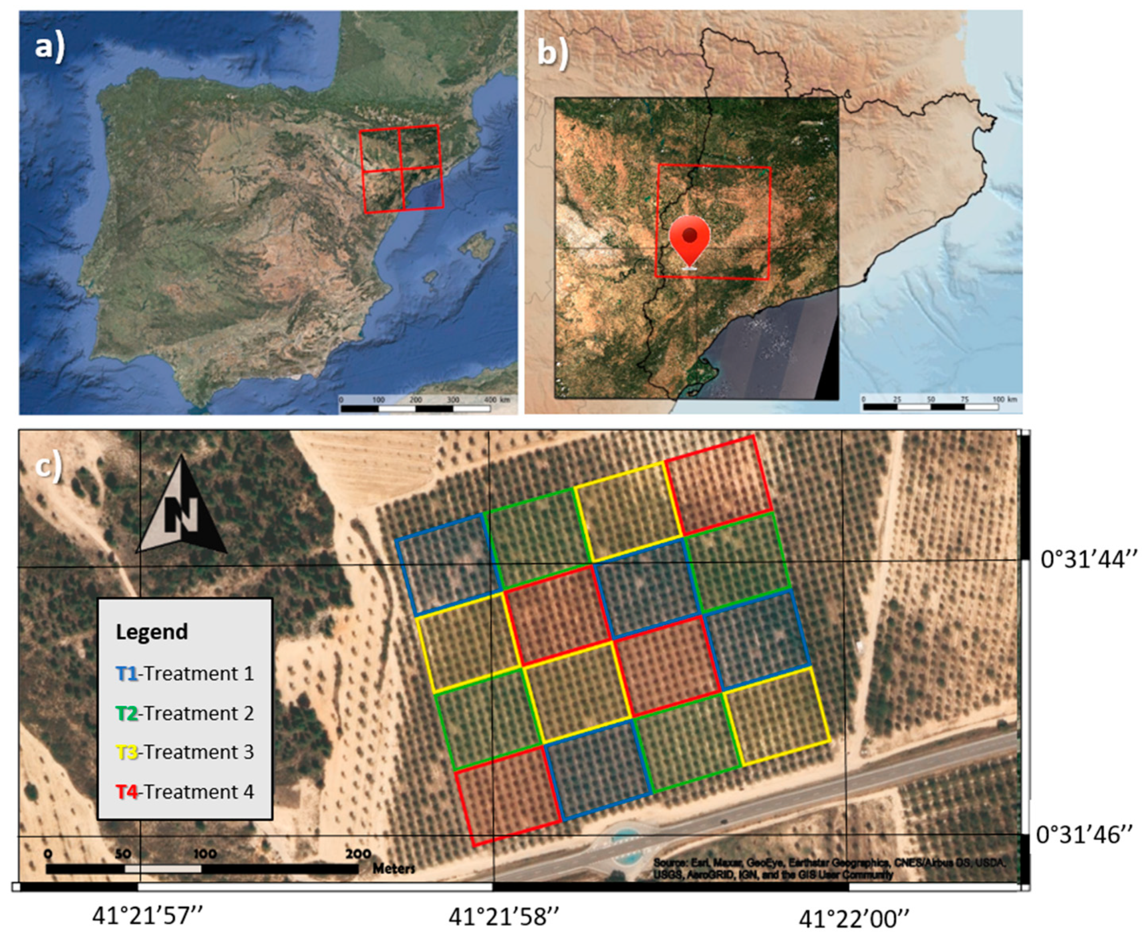
2.1. Study Site

The experiment was carried out in a 7.5 ha almond orchard located in Maials, Spain (41°22.9′172″N, 0°31.27′619″E) from 2017 to 2020 (see Figure 1). The climate in the region is typically Mediterranean with a mean annual temperature of 14.5 °C and average annual precipitation of 307.9 mm, mainly occurring during autumn (October–December) and spring (March–June). The accumulated average reference evapotranspiration (ET0) during the growing season (March–October) was 960 mm. Soil type is loamy with a slightly calcaric influence due to the petrocalcic origins of the rock. Soil depth varied from 120 to 180 cm, depending on the area. Almond tree management for pruning; disease and pest control; and soil management and fertilisation was based on Spanish integrated production management practices [48].

2.2. Field Experimental Design
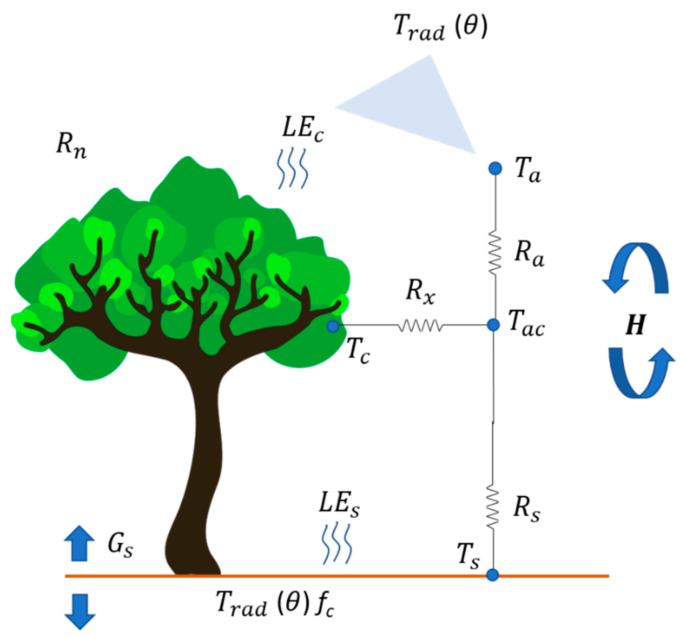
Almond trees (cv. Vairo) were grafted onto GF-677 rootstock and planted in 2015 in a 6 × 6 grid (277 trees/ha). Two drip irrigation laterals were placed 80 cm away from the tree rows in 2018. In 2019, the laterals of treatment T4 were moved to 70 cm from the tree rows. Drippers were separated and placed 75 cm apart and discharged 25.6 L/h through pressure-compensating emitters per tree. Irrigation was scheduled on a weekly basis and conducted on a daily basis. Crop water requirements (ETc) were calculated following the methodology proposed by Girona et al. [15]. The Penman–Monteith ET0 was obtained from the closest weather station from the Meteorological Service of Catalonia (SMC), which was located 3.5 km from the orchard (www.ruralcat.net/web/guest/agrometeo.estacions, accessed on 15 July 2021). The crop coefficients (Kc) were adapted from Goldhamer and Girona [49] and the shading factor (Kr) was taken from Fereres et al. [50]. Therefore, irrigation was performed to replace crop evapotranspiration (ETc) minus effective precipitation (Peff).
A randomized complete block design with four block replicates was used. Each block housed four experimental plots with 80 trees in each. Four differential irrigation treatments were adopted: Treatment 1 (T1) consisted of simulating a scenario with seasonal water availability of 9000 m3/ha. During the four years of this study, these trees never reached this water demand, so T1 was always fully irrigated. Treatment 2 (T2) consisted of simulating a scenario with seasonal water availability of 6500 m3/ha. During the first two years of this study, the trees did not reach the pre-established water demand and so were fully irrigated. However, during 2019 and 2020, sustained deficit irrigation was adopted which consisted of gradually reducing the crop water requirements to 25% ETc over the course of the growing season. Treatment 3 (T3) consisted of simulating a scenario with seasonal water availability of 4500 m3/ha. In 2017, almond water demand was below this threshold, and so in this year the trees were fully irrigated. In 2018, a moderate sustained deficit was adopted which consisted of reducing water prescriptions by 10% ETc. In 2019 and 2020, irrigation was scheduled based on a reduction by 35% ETc. Finally, treatment 4 (T4) consisted of simulating a scenario with seasonal water availability of 2500 m3/ha. In 2017, almond water demand was below this value, and so the trees were fully irrigated. However, sustained deficit irrigation was applied in all the other years, which consisted of reducing the amount of water to below 2500 m3/ha. To achieve this, reductions by 40% ETc in 2018 and by 60% ETc in both 2019 and 2020 were applied. Peff was calculated as half of the rainfall for a single event day with more than 10 mm of precipitation, or was otherwise considered to be zero. The total amount of water applied was measured weekly using digital water meters (CZ2000-3M, Contazara, Zaragoza, Spain).

2.3. TSEB Scheme

Most energy balance approaches assume that the total available energy in the surface (net radiation (Rn)–soil heat flux (G)) is partitioned into sensible heat flux (H) and latent heat flux (LE), neglecting other sources of heat dissipation such as biochemical changes (i.e., photosynthesis, respiration) or heat stored in the canopy due to their low contribution in proportion to the overall energy budget.
R n = H + G
The TSEB is a model formulated originally by Norman et al. [30] and was afterward modified and improved by Kustas and Norman [51]. In TSEB, each of the components of the energy balance equation is partitioned into canopy and soil, except for G, as it assumes negligible heat storage at the canopy layer.
R n = R n c + R n s
R n c = L E c + H c
R n s = L E s + H s + G
Equation (2a–c) represent the partition of the latent heat of evaporation (LE), where the subscripts c and s refer to canopy and soil, respectively. G is estimated as a fraction of soil net radiation [52].
G = c G R n s
The fraction of net radiation which is stored in the soil c G is dependent on the type of soil, soil moisture and time of the day, but typically is set as 0.35 for near-noon conditions [30]. There are other approaches that set G as a function of daytime [53], but for this study it is assumed that using a constant fraction, as in Equation (3), is still valid as the satellite overpasses are within the 2–3 h around solar noon.
Sensible heat flux is partitioned into soil and canopy in which fluxes between soil and canopy are connected in series, as shown in Figure 2, following an analogy of Ohm’s law for electric transport.
H s = ρ c C p T s T a c r s
H c = ρ c C p T c T a c r x
H c + H s = H = ρ C p T a c T a r a
In Equation (4a–c) the sensible heat flux is partitioned into soil and canopy, where ρ is the density of air, C p is the specific heat of air, T s is the soil temperature, T a is the air temperature, T a c is the temperature in the canopy air space (equivalent to the aerodynamic temperature), r s and r x are the surface boundary layer resistances to heat transfer from the soil and canopy, respectively, to the air-canopy layer, and r a is the aerodynamic resistance to heat transport between the air-canopy layer and the overlying air layer.
These resistances represent the impediment or the enhancement of vertical heat and water transport related to the degree of air turbulence. Therefore, they mainly depend on wind speed, atmospheric stability (i.e., convective transport) and canopy/soil structure (i.e., surface roughness and wind attenuation through the canopy). Although there are several approaches to quantify these resistances [51,54,55], and several parameters that could be fitted [56], we used the original resistance formulation proposed in TSEB [51] with their standard coefficients in order to guarantee the operational aspect of the TSEBS2-S3 approach as proposed by Guzinski et al. [43,44,46].
Figure 2. TSEB sensible heat model scheme (adapted from [57]).
Remotesensing 14 02106 g002
Soil and canopy temperatures cannot be directly retrieved from coarse-resolution satellite-derived images. However, the directional radiometric temperature observed by the sensor can be considered to be a mixture of warm soil and cool vegetation:
T r a d ( θ ) = [ f c ( θ ) T c 4 + ( 1 f c ( θ ) ) T s 4 ] 0.25
with f c ( θ ) as the fraction of vegetation observed by the thermal infrared sensor at a zenith angle of θ .
In order to derive Tc and Ts, the Priestley–Taylor (PT) approach is applied [30,58] and an initial maximum potential rate of transpiration is set.
λ E c = α P T f g Δ Δ + γ p R n c
where Δ is the slope of the saturated vapor pressure to the air temperature, γ p is the psychometric constant, and f g is the fraction of leaf area index (LAI) that is green and is therefore transpiring. The α P T coefficient is set to 1.26. With this first guess of LEc known, together with Equations (2b), (4b) and (5), it is possible to obtain an initial estimate of T s and therefore of LEs, using Equations (4a) and (2c). LEs at this stage usually yields negative values, which would mean there is condensation in the soil. This situation is not expected at daytime, i.e., at satellite overpass time, and is caused by the fact that LEc is probably below its potential rate due to any degree of stress in plants. In that case, LEc is iteratively recalculated by sequentially reducing the α P T coefficient value until both LEs and LEc become zero or positive.
Further details on the TSEB model scheme can be found at the source code (https://github.com/hectornieto/pyTSEB. DOI: 10.5281/zenodo.594732, last accessed on 20 August 2021) and the original formulation of the model [30].

2.4. Input Data

2.4.1. Image Acquisition

For this study, high-resolution shortwave observations acquired by the Multispectral Instrument (MSI) mounted on Sentinel-2A and 2B tandem satellites were used. MSI acquires shortwave radiance information in 13 spectral bands with a spatial resolution of 10 m, 20 m or 60 m, depending on the spectral band, and there is a global geometric revisit of at least five days when both satellites are considered, and higher as latitude increases. The MSI differs from previous open data medium-resolution multispectral sensors by including three spectral bands in the red edge part of the electromagnetic spectrum. The red edge responds highly to chlorophyll content as these bands are sensitive to leaf pigments. It also includes the traditional visible and near-infrared bands and two bands in the shortwave infrared, which are sensitive to water content. Sentinel-2 images at Level-2A (L2A; bottom of atmosphere reflectance) were directly retrieved from CREODIAS (https://creodias.eu/, accessed on 20 October 2021), downloading four tiles for this study (T31(TBF, TCG, TBG, TCF)). In order to have a larger dataset of an agricultural area for the sharpening algorithm and improve the accuracy of the machine learning model, the whole area of Lleida (northeast of Spain) (273,940, 4,573,440, 359,220, 4,653,320 m UTM 31 N) was processed and mosaicked to retrieve the biophysical parameters required by TSEB at 20 m spatial resolution. Since the 10 m resolution bands of S2 are not required in this study, band 8, which is a broader bandwidth version of band 8A, was excluded for this study.
The S3 SLSTR sensor was used to obtain the thermal data. This includes three thermal infrared (TIR) channels with 1 km nominal spatial resolution and less than two days temporal resolution with one satellite at the equator and half a day when Sentinel 3A and B are available (April 2018). The LST was obtained directly as an L2A product of S3 SLSTR at 1 km resolution. All the available images acquired in the 10 days ahead of an S2 acquisition in the first semester of 2017 and all SLSTR LST data with 5 days ahead from the second semester of 2017 to the end of 2020 were downloaded. A total of 175 S2 dates and 714 S3 cloud-free scenes were fetched from March 2017 to October 2020.
Landsat-8 is currently the satellite LST source at high spatial resolution, since it includes several bands in the shortwave spectrum at field-scale resolution plus a high-resolution thermal band (100 m). The main issue with Landsat-8 is that it only overpasses every 16 days. Temporal resolution is essential when monitoring ET, mainly because the ET dynamics can change within short temporal windows. If Landsat-8 imagery is available in a turnaround time of 16 days, relevant ET information is likely to be lost. Moreover, there is the risk of cloud occlusion during the satellite overpass cycle, which may lead to not having a clear image in more than a month. Therefore, in the present study, Landsat-8 LST was used as the benchmark TSEB product for which results from TSEBS2+S3 could be compared against.

2.4.2. Sentinel-2 Biophysical Parameters of the Vegetation

From the S2 images, the vegetation biophysical parameters were computed through the Biophysical Processor [59] available in the SNAP software v8.0 (https://step.esa.int/main/download/snap-download/—last accessed on 10 June 2021). This processor relies on building a randomized dataset of vegetation biophysical variables from which reflectance simulations by the radiative transfer models (RTM) PROSPECT [60] and SAIL [61] are produced. Then, the simulated reflectance values are trained against the biophysical parameters through a machine learning approach. The trained model is hence used to predict effective values of green LAI, fractional vegetation cover (FVC), fraction of absorbed photosynthetically active radiation (FAPAR), canopy chlorophyll content (CC) and canopy water content (CW) over the actual S2 image. The derived values of CC and CW are then used to derive the leaf optical properties, using CC for the transmittance in the visible spectrum and CW for the transmittance in the infrared spectrum. These transmittances are used to estimate net radiation and its partitioning into canopy and soil using the Campbell and Norman model [51,62]. As an additional outcome from these outputs, the fraction of green vegetation (fg) is derived by combining information of LAI and FAPAR [45]. In order to avoid inconsistencies in estimation and cloud-related issues, the multi-step Savitzky–Golay filtering algorithm [63] was used to smooth the S2 LAI data, and the upper envelope of LAI time series was generated.

2.4.3. Sharpening Land Surface Temperature (LST)

The S3 SLSTR LST images were disaggregated using the DMS approach [43,45]. The sharpening objective is to downscale the 1 km LST imagery from the S3 to the S2 spatial scale (20 m). This methodology relies on the empirical relation that exists between shortwave and thermal data. Similar approaches describe some relations between these two regions, such as TsHARP, which relates the normalized difference vegetation index (NDVI) with thermal data [64] or even with other vegetation indexes (VIs). The main limitation to these previous studies is that the full multispectral information was not represented in VIs but only a small part of it, since they only use two or three bands of the sensors [45]. Often they assume linear relations and, in most cases, these relations are non-linear. The DMS technique instead uses a non-parametric approach that considers a full set of spectral bands and ancillary information (e.g., elevation, exposure, etc.). In addition, it uses a machine learning algorithm that permits non-linear relations between shortwave and thermal data and ensures the conservation of emitted thermal energy between the sharpened and the original LST data by a bias correction approach. DMS aggregates the high-resolution image to the thermal image coarse resolution, and afterwards builds a machine learning model using the most homogeneous coarse-resolution pixels in the scene. In that way, urban areas, roads and highly heterogeneous landscapes can be discarded in the training dataset [65].
The machine learning algorithm used in this study for the non-parametric relation was a decision tree as it is fast and at the same time reliable in comparison with other algorithms such as neural networks [44]. The pyDMS Python module (https://github.com/radosuav/pyDMS last accessed on 20 October 2021) was used to apply this algorithm.

2.4.4. Meteorological Data

Meteorological data from the ERA5-Land reanalysis dataset of the Copernicus Climate Change Service (C3S) (2019) were used. These data are extremely useful for running energy balance models at regional and basin scale as they consist of hourly gridded information at 0.1° of spatial resolution and contain several layers of meteorological data. For the current study, the variables used were air temperature at 2 m, dew point temperature at 2 m, wind speed at 10 m, surface pressure and total column water vapor (TCWV).

2.4.5. Ancillary Data

Vegetation height and leaf inclination angle cannot be retrieved from remote sensing passive data directly. The leaf angle distribution parameter indicates how leaves are oriented in the vertical plane. This is important when accounting for determining the beam shortwave net radiation partitioning [66]. For almond, it is assumed that leaf angle follows a spherical distribution [67] in which the leaves point in all directions equally. Canopy height was measured periodically per plot, ranging from 2.3 m in the stressed plots (T3 and T4) to 5 m in the most irrigated ones during the last year of the study (T1 and T2). This variable, together with LAI, has an impact on the aerodynamic roughness [68], which in the TSEB scheme determines the atmospheric stability and aerodynamic resistance used to estimate the sensible heat flux.

2.5. Daily ET Upscaling

Instantaneous energy fluxes at the satellite overpass time were estimated using TSEB with the previously described inputs. Then, the latent heat flux was integrated into the daily evaporation rate. To achieve this, the instantaneous value, in W/m2, was upscaled to daily water fluxes, expressed in units of mm/day, by multiplying the instantaneous ratio of latent heat flux over solar irradiance by the average daily solar irradiance [69].

2.6. Gap Filling

It is a well-known issue that clouds can partially or totally occlude satellite optical images. Due to the S2+S3 synergy methodology, it is possible to have occlusion either on S2 high-resolution images or on S3 coarse-resolution images. If there is an occlusion with S2 data, it will extend for the following 5-day window or until an unoccluded image is available. If the occlusion corresponds to clouds in an S3 image, the period of occlusion will be shorter, but each masked area will correspond to 1 km pixel.
To obtain a continuous dataset with daily ETa values, a crop stress coefficient (Kcs) was retrieved from the valid ET estimates by computing the ratio between actual and reference ET, with the latter computed from the meteorological gridded data.
K c s = ET a ET 0
This ratio ( K c s ), which represents the combined effect of the FAO-56 crop and stress coefficients ( K c s = K c K s ), is used to fill the cloud gaps present in the following days, under the assumption that Kcs will remain constant for a short-term period [46].

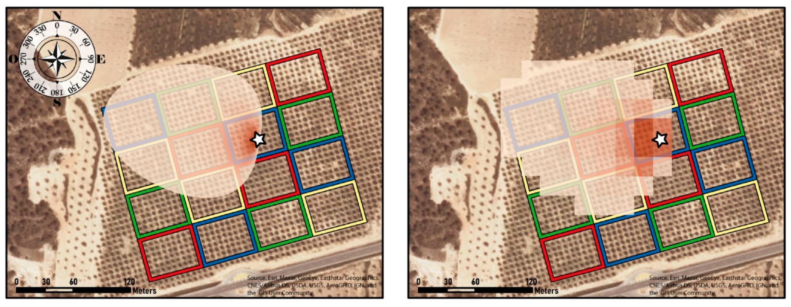
2.7. Eddy Covariance (EC) Fluxes

To validate the modelled energy fluxes, an eddy covariance (EC) system was set up at the study site, equipped with an open path infrared gas analyzer (LICOR-7500), a sonic anemometer (CSAT3), a four-component net radiometer (NR01 Campbell) and four soil heat flux plates (Hukseflux) located at 0.5, 1, 1.5 and 2 m from the tree line. A CR3000 Campbell datalogger was used to store the 20 Hz measurements as well as the half-hourly aggregated fluxes. The fluxes were corrected by the Webb, Pearman and Leuning (WPL) method described in Foken et al. [70] to correct density fluctuations in open path gas analyzers. Then, the 30-min period fluxes in which the S3 overpassed (~10:30 local time) were used. For solving the non-closure of the energy fluxes, one closure forcing option is to apply the Bowen ratio closure method, which assumes that the ratio between H and LE (β = H/LE) is correctly measured by the EC system so that individual values of these fluxes can be adjusted to balance Equation (1) [71,72].
To estimate the relative contribution of each pixel to the measured fluxes, it is mandatory to calculate the tower footprint. This footprint will depend on the wind direction and speed and the surface roughness, which is mainly driven by the vegetation structure in the surroundings. The footprints were estimated using a two-dimensional parametrization of the flux footprint predictions ([73]; www.footprint.kljun.net last accessed on 19 September 2021). Then, the footprints were resampled to 20 m to match S2 resolution (Figure 3). Finally, the latent heat flux and the sensible heat flux were aggregated as a weighted sum of the pixel contribution to be compared against the tower fluxes. However, the R n footprint from the net radiometer covers only an area encompassed by the sensor viewing angle, which in this case falls in the site where the eddy covariance is set (i.e., T1).

2.8. Model ETa Intercomparison through a Soil Water Balance Approach

Average evapotranspiration for the period between two soil water content (SWC) measurements was estimated from the following equation:
ETa WB = IR + Peff − ΔSWC
where WB is water balance, IR is irrigation, Peff is effective precipitation and ΔSWC is the difference of soil water content between two measurements. Since the soil has a high infiltration rate and null slope, runoff was assumed to be zero and, therefore, Peff was calculated as described above. Then, in order to compare values of ETa between irrigation treatments and with the TSEBS2+S3 approach, ETa WB was normalized by dividing the total ETa of a specific period by the number of days between two consecutive measurements.
A neutron probe (Campbell Pacific Nuclear Scientific, Model 503) was used to measure SWC down to 150 to 180 cm in one plot in each irrigation treatment. In each plot, three tubes were installed, one in the emitter-wetted area, a second in the middle of the lane, and a third in an intermediate location between rows. Readings were taken at 20 cm intervals every 15 to 20 days throughout the growing season. In total, the number of measurements ranged from eight to twelve, depending on the growing season. The neutron probe was calibrated for the experimental soil by taking soil samples for volumetric moisture content (ɵ, cm3 of water/cm3 of soil) when the access tubes were installed.
Both TSEBS2-S3 and the SWB approach were intercompared by computing their correlation as well as their root mean squared deviation ( RMSD = ( x i y i ) 2 N ) . RMSD is analogous to RMSE but it denotes deviations between two independent estimates (x and y), rather than errors from one estimate to a reference measurement.

3. Results

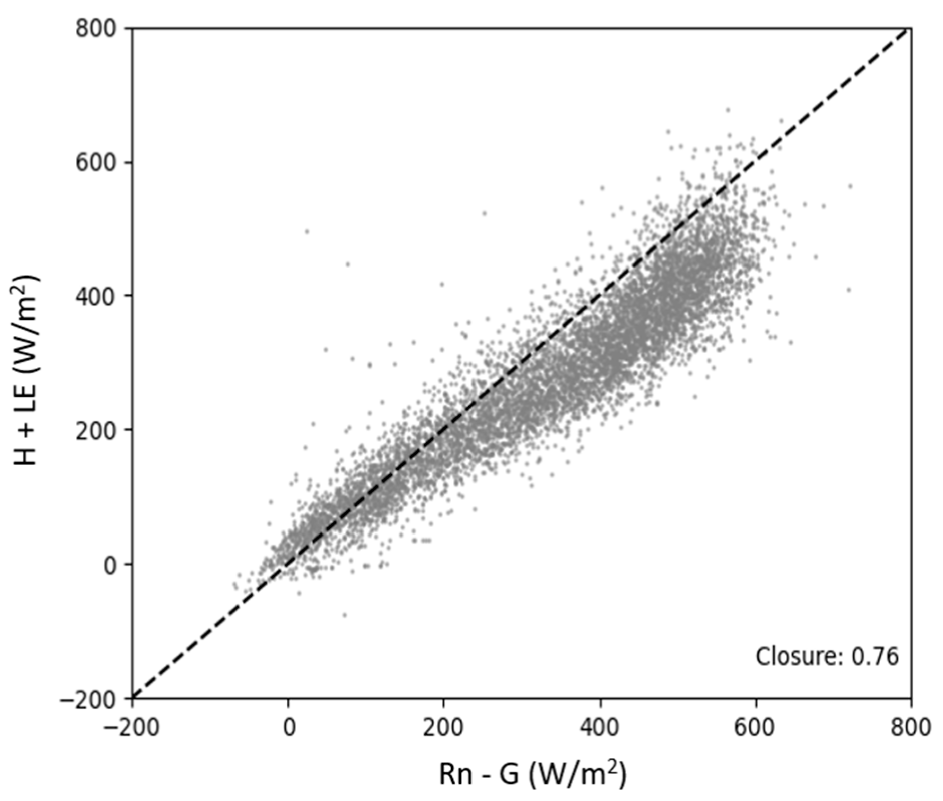
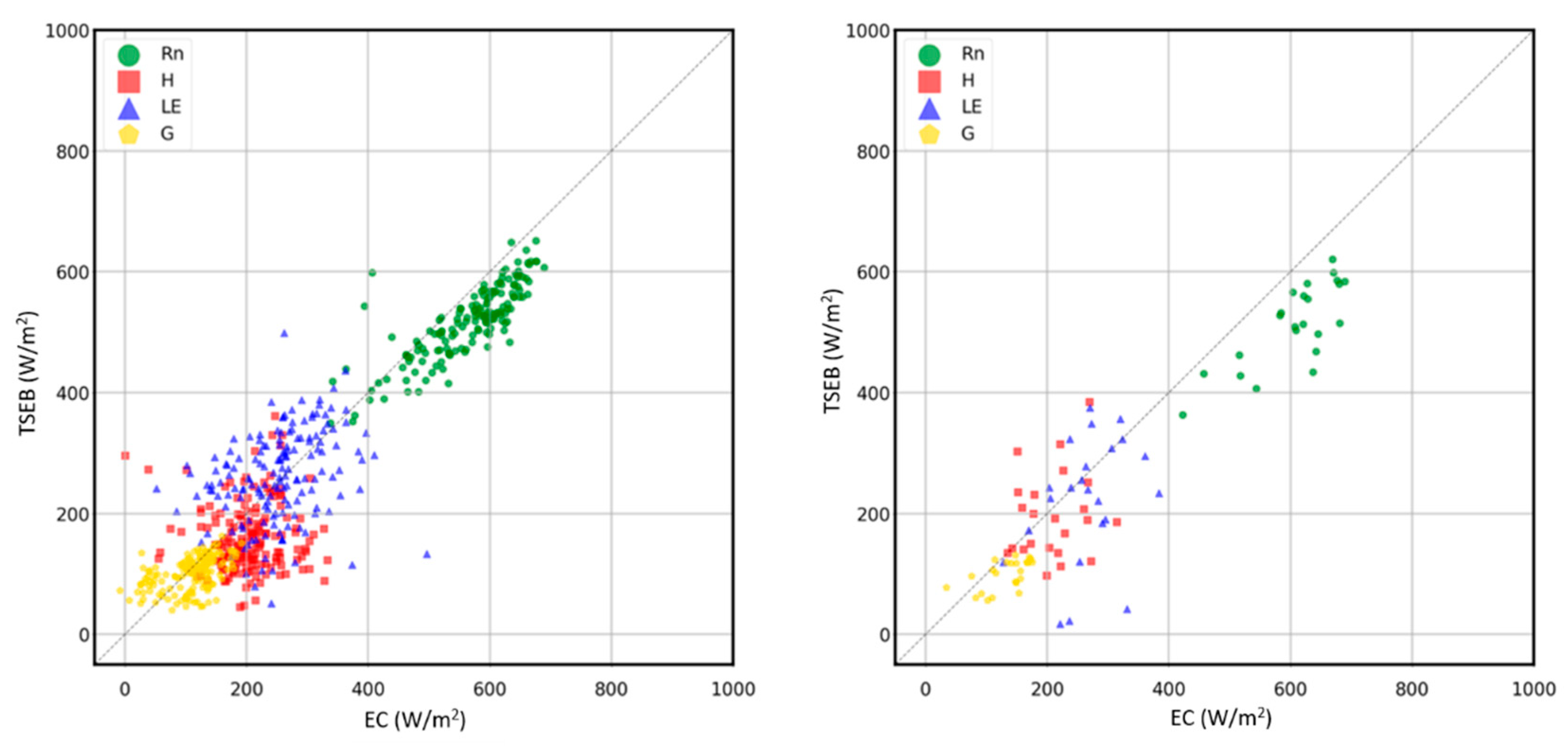
3.1. Validation with the Eddy Covariance Flux Tower

The eddy covariance closure was analyzed in order to observe the reliability of measured fluxes. Figure 4 shows the closure at daytime hours (8:00–18:00) out of this time range. The value of the slope of the closure was 0.76, excluding night, dusk and dawn observations, which falls within the range of typical values found, for instance, in the FLUXNET database [74], of between 0.56 and 0.97 [75]. Usually, EC-derived fluxes bring inconsistencies, especially at dawn and dusk. There is better closure when the available energy is lower than 300 Wm−2 associated with morning hours, while at high irradiance, estimates of H+LE were up to 25% lower than Rn-G. The average Bowen ratio at the satellite overpasses was 0.74, being higher in July–August, when it rose above unity, due to the arid conditions of these months when temperatures can reach up to 40 °C or more.
The energy balance fluxes from TSEB using the S2+S3 method (TSEBS2+S3) were evaluated against eddy covariance measurements from 2018 to 2020 during the vegetative growing period (March–October) (Figure 5, Table 1). Net radiation appears to be slightly underestimated by TSEBS2+S3 with an RMSE of 63 W/m2. Sensible heat flux has an RMSE of 90 W/m2, LE of 87 W/m2, and G an error of 37 W/m2. Turbulent fluxes are the most scattered ones. Rn shows a bias of −46 W/m2 that corresponded to the −43 W/m2 underestimation of sensible heat flux from TSEBS2+S3 over the EC. High values in LE measured by the EC tower are related to dates after a precipitation event where the tower measured high LE in contrast with TSEBS2+S3; this sharpening approach may not identify the sharp surface temperature decrease due to the larger evaporation from the soil. Soil heat flux appears to be overestimated by TSEBS2+S3 at lower fluxes and overestimated for higher net radiation days.
The energy fluxes estimated from TSEB using Landsat LST (TSEBLandsat) were also compared against the eddy covariance data. The error fluxes derived from TSEBLandsat (RMSE; Rn: 103 W/m2, H: 80 W/m2, LE: 108 W/m2, G: 43 W/m2) did not differ significantly from TSEBS2+S3, showing the same pattern for net radiation. Even a higher error can be observed, which is hard to determine given the fewer observations compared to TSES2+S3. Observing the distribution pattern, it could be assumed that there is no significant improvement in using a higher-resolution thermal sensor at this scale, where spatial heterogeneity is under the 100 m resolution, or the sharpening technique can identify these differences by determining the actual relationships between stressed and non-stressed vegetation for the training area in the corresponding time window.

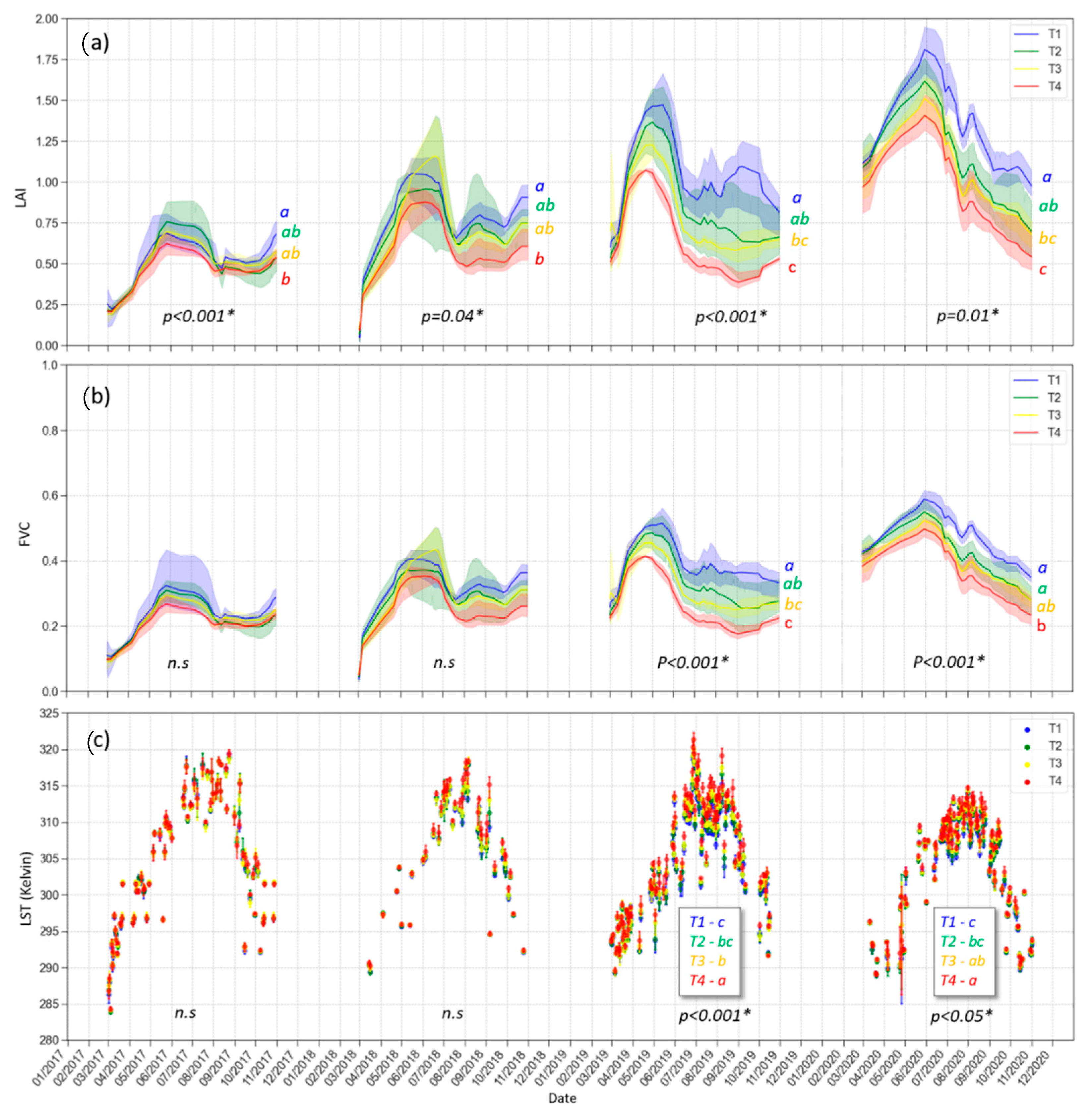
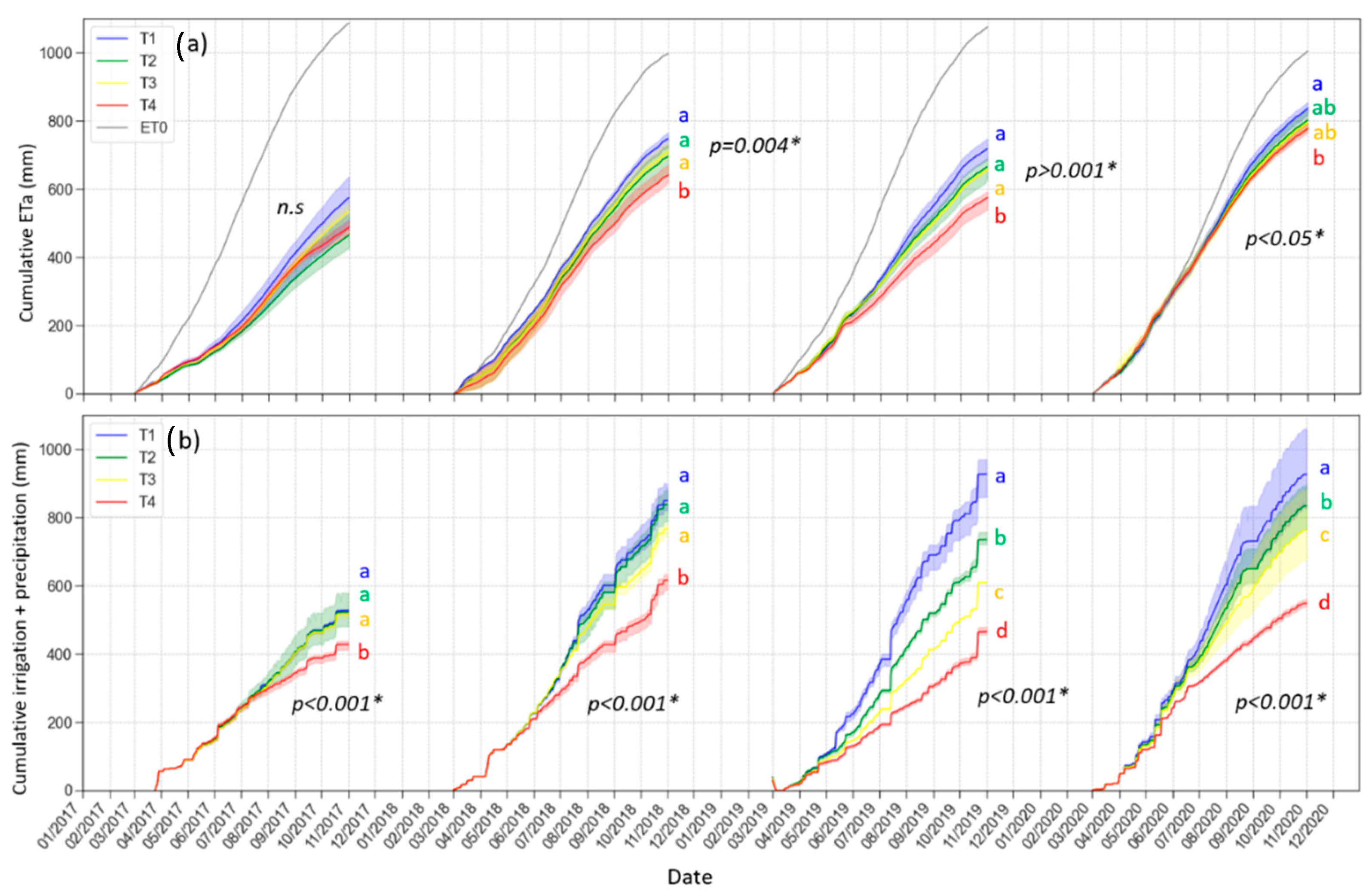
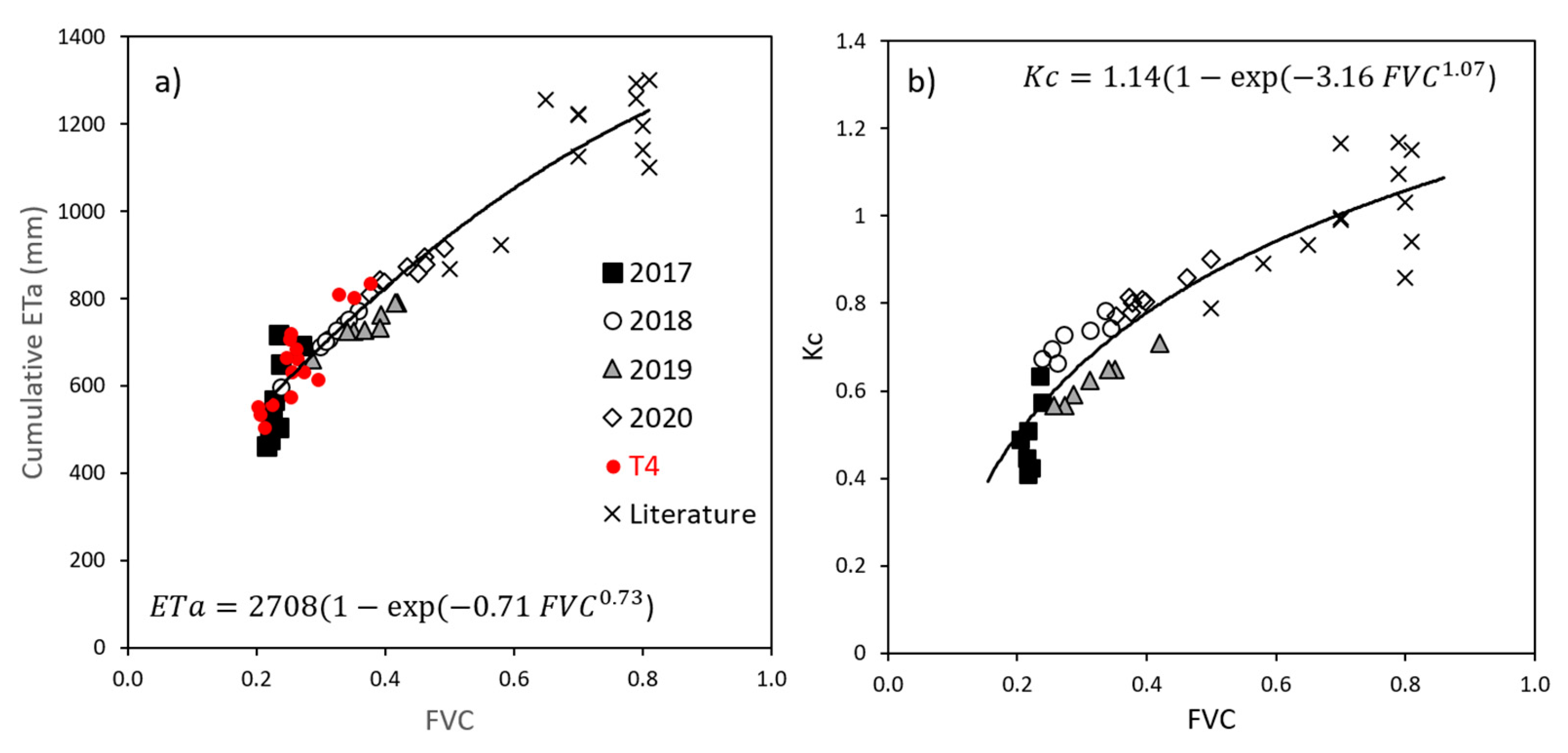
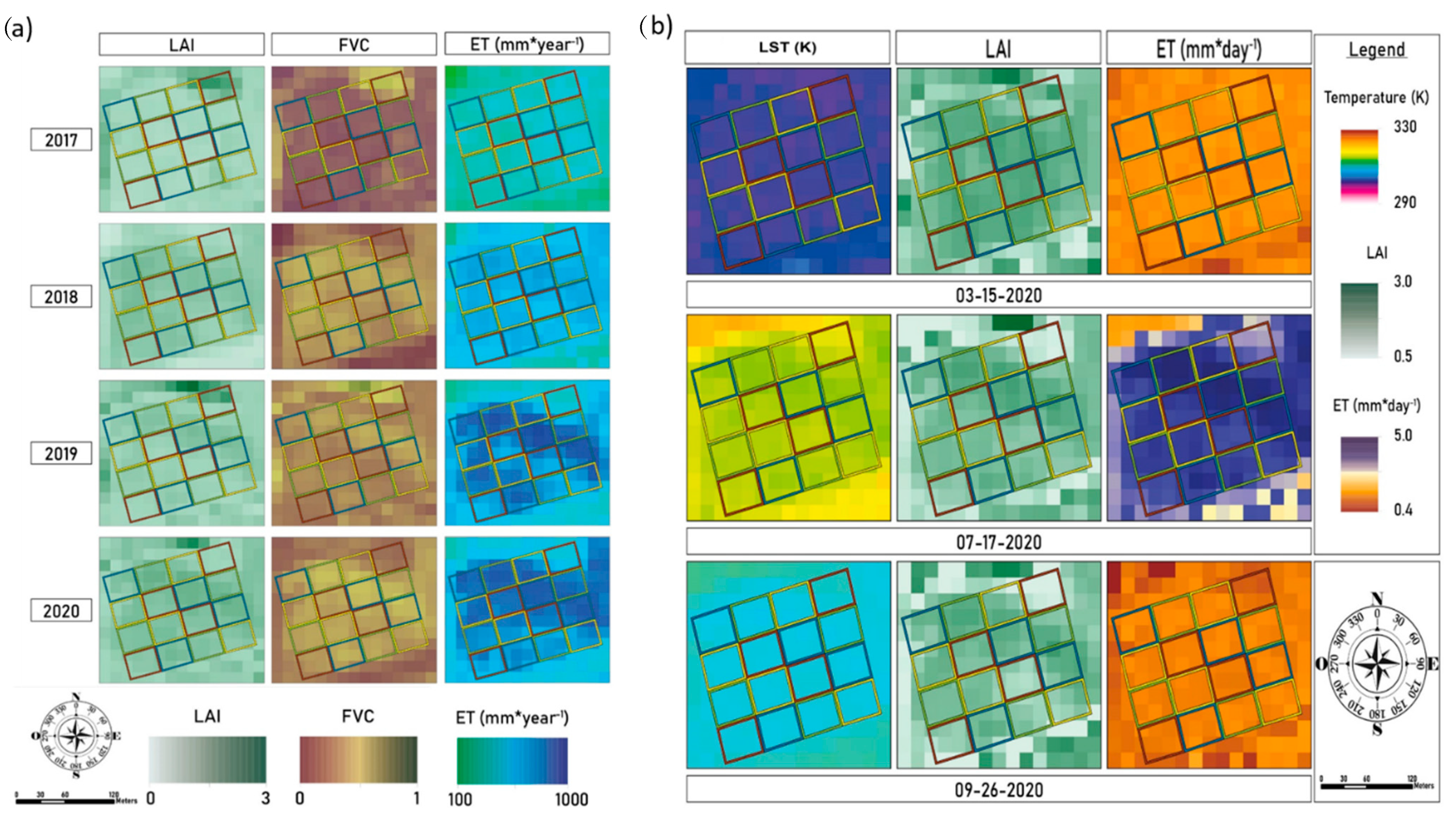
3.2. Water Applied and Biophysical Parameters of the Vegetation

Reference ET (ET0) is a proxy for atmospheric demand, as it is usually modelled over well-irrigated grass, depending only on meteorological conditions. In the orchard location, ET0 was higher in 2017 and 2019 by 100 and 90 mm, respectively, in comparison to 2018 and 2020. The two latter years corresponded to years with higher precipitation (Table 2).
The irrigation period started the second week of March for all treatments and years. The amount of water applied in 2017 was similar for all treatments, except for T4 which received 28% less water in comparison to other treatments. In 2018, differences between T4 and other treatments were also significant. Irrigation differences for T3 in comparison to other treatments can be observed in 2018, probably due to the high rainfall, but were not significant. In 2019 and 2020, the differences were significant between all treatments. The amount of water applied in T2, T3 and T4 in comparison to T1 was, respectively, 26%, 43% and 63% less in 2019, while in 2020 it corresponded to 10%, 25% and 55% less.
With respect to the biophysical parameters of the vegetation, the LAI is one of the most important when accounting for canopy size and vigor, and is used as input in TSEB. Figure 6 shows the time series of S2 LAI values after applying the Savitzky–Golay interpolation filter for each irrigation treatment during the four-year study. There is a clear increase in vegetative growth from the first year of study to 2020, increasing from averaged maximum LAI values of 0.75 in 2017 to 1.80 in 2020 (Figure 6a). A seasonal trend of LAI can also be observed representing crop development at the beginning of each growing season and leaf senescence at its end. A peak can be seen by the end of spring, when vegetative growth of the almond trees coincided with maximum vegetative development of the cover crop in the interrow. Differences between treatments were also noticeable in some years. In 2017, no significant differences were observed between treatments. In 2018, T4 had significantly smaller LAI values in comparison to other treatments (p < 0.01). In 2019, differences in LAI between treatments were more evident and significant differences were observed between all treatments (p < 0.01). In comparison to T1, the seasonal average LAI decreased 18%, 25% and 40% for T2, T3 and T4, respectively. In 2020, significant differences were observed between T1 and T3 and T4, and also between T4 and T2. In comparison to T1, the seasonal average LAI decreased 18% and 33% in T3 and T4, respectively. Although FVC is not used by TSEB, as vegetation gap fraction is modelled in TSEB from LAI and the clumping index [51], several studies have demonstrated high correlation with crop evapotranspiration [4,76]. Therefore, in this study, we also wanted to assess the seasonal pattern of FVC for different irrigation treatments. As was expected, results showed a similar pattern to that observed for LAI (Figure 6b). Sharpened LST at 20 m resolution was also compared between treatments (Figure 6c). Non-significant differences in LST were observed in the first two years of the experiment. However, LST of T1 and T4 showed significant differences, respectively showing the lowest and highest values in 2019 and 2020 in comparison to other treatments. These differences mostly occurred during the summer time, when there is a higher atmospheric demand and differences between well-watered and stressed treatments were more evident.

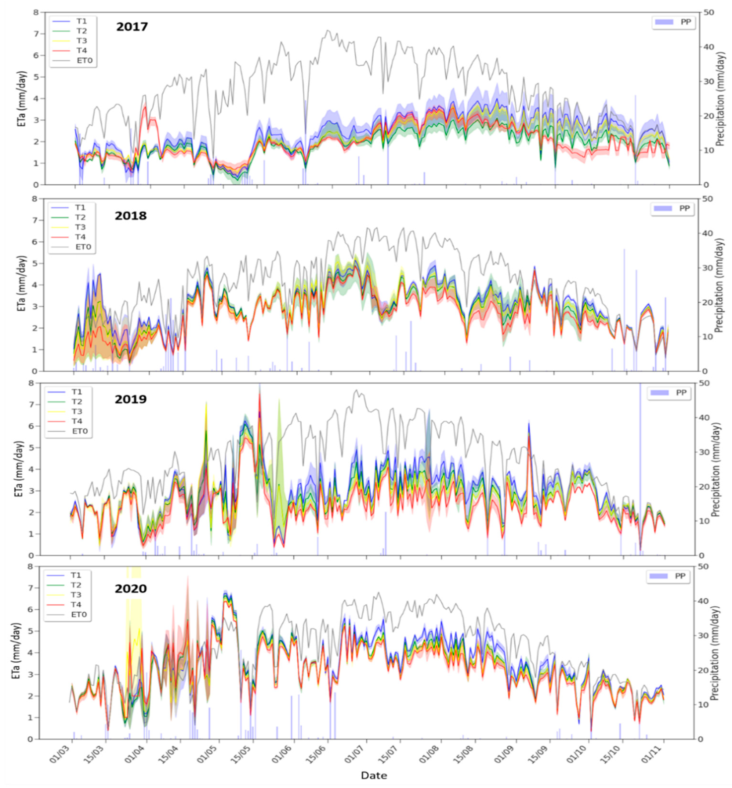
3.3. Seasonal Trend of Actual Crop Evapotranspiration

Figure 7 shows the seasonal evolution of the modelled ETa with TSEBS2+S3 for each irrigation treatment, using the gap-filling procedure. ETa increased sharply from early March to mid-June, when maximum values of ~4 to 5 mm/day were attained, depending on the year. After mid-July, ETa progressively dropped until the end of the season as ET0 and LAI also decreased. It can also be seen how ETa values drop for those days with precipitation events, due to lower solar irradiance under cloudy conditions (lower ET0), after which ETa rapidly ramps up in sunny days as soil moisture is replenished. As expected, ETa increased year after year as vegetative growth increased, but also depending on seasonal ET0. On average, the highest ETa values were observed in 2020 due to the higher LAI values. In 2017, no significant differences between treatments were observed, except at the end of the growing season when ETa of T4 was significantly lower. This coincided with a decrease in the irrigation amount of water from mid-July until the end of the growing season. ETa values were all below 4 mm/day. In 2018, significant differences between T4 and other treatments were also observed from 15 July. A similar pattern was observed in 2019 and 2020.
With respect to total cumulative ETa throughout the growing season, differences between treatments were significant from 2018 (Figure 8a). In 2018, a total of 682 mm was evaporated in T4, which was 9–14% less in comparison to other treatments. In that year, the sum of irrigation and rainfall water applied in T4 was also ~20% less than in the other treatments (Figure 8b). In 2019, differences in cumulative ETa between treatments were also significant. Despite the significant differences in the amount of water applied between all treatments, a significant decrease in ETa was only observed in T4, ranging between 20% and 13% less evaporated water. Although it was expected that the highest differences between treatments would be observed in 2020, these were not as evident as in 2019, probably due to a lower ET0 and higher number of precipitation events. Cumulative ETa for T4 was ~8% less in comparison to other treatments. Results also showed that T4 almond trees evaporated 8%, 10%, 22% and 36% more than the amount of water applied respectively for 2017 to 2020, while for T1 and T2 the total amount of water applied was higher than that consumed by the crop. Therefore, differences in ETa between treatments and years demonstrate the ability of this approach to identify periods of water stress and peaks over the growing season.

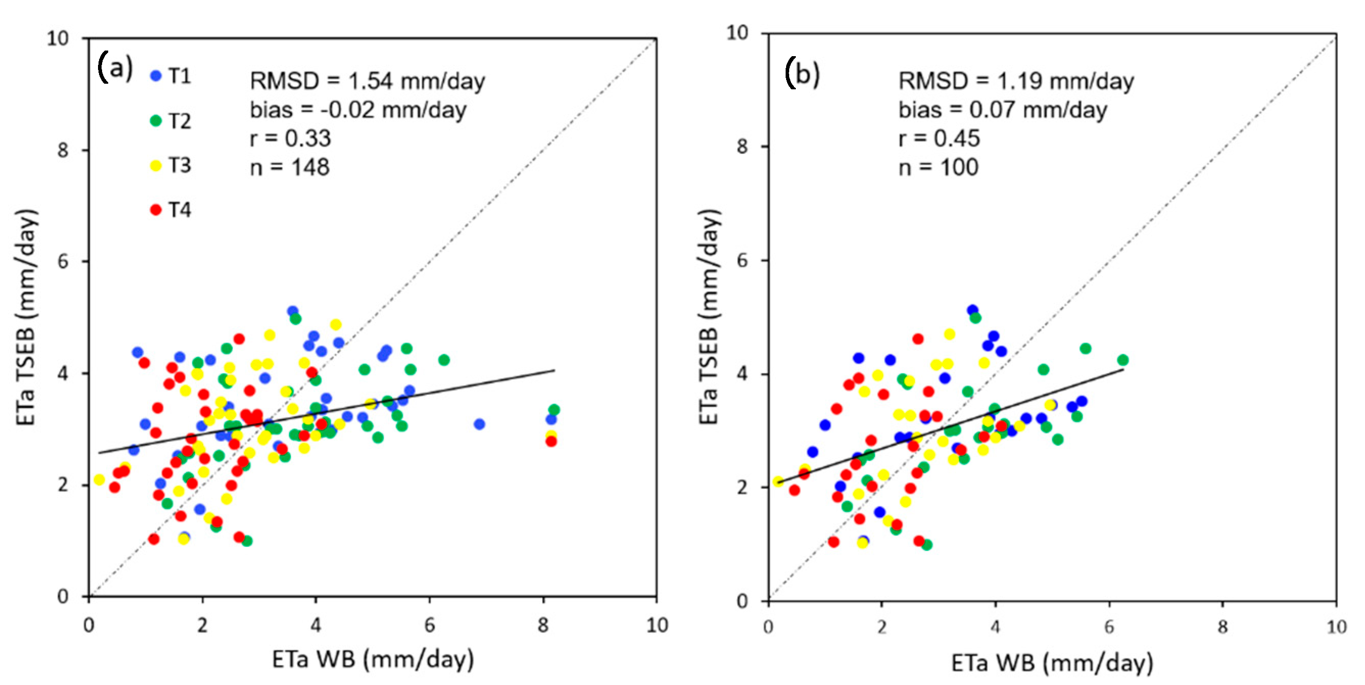
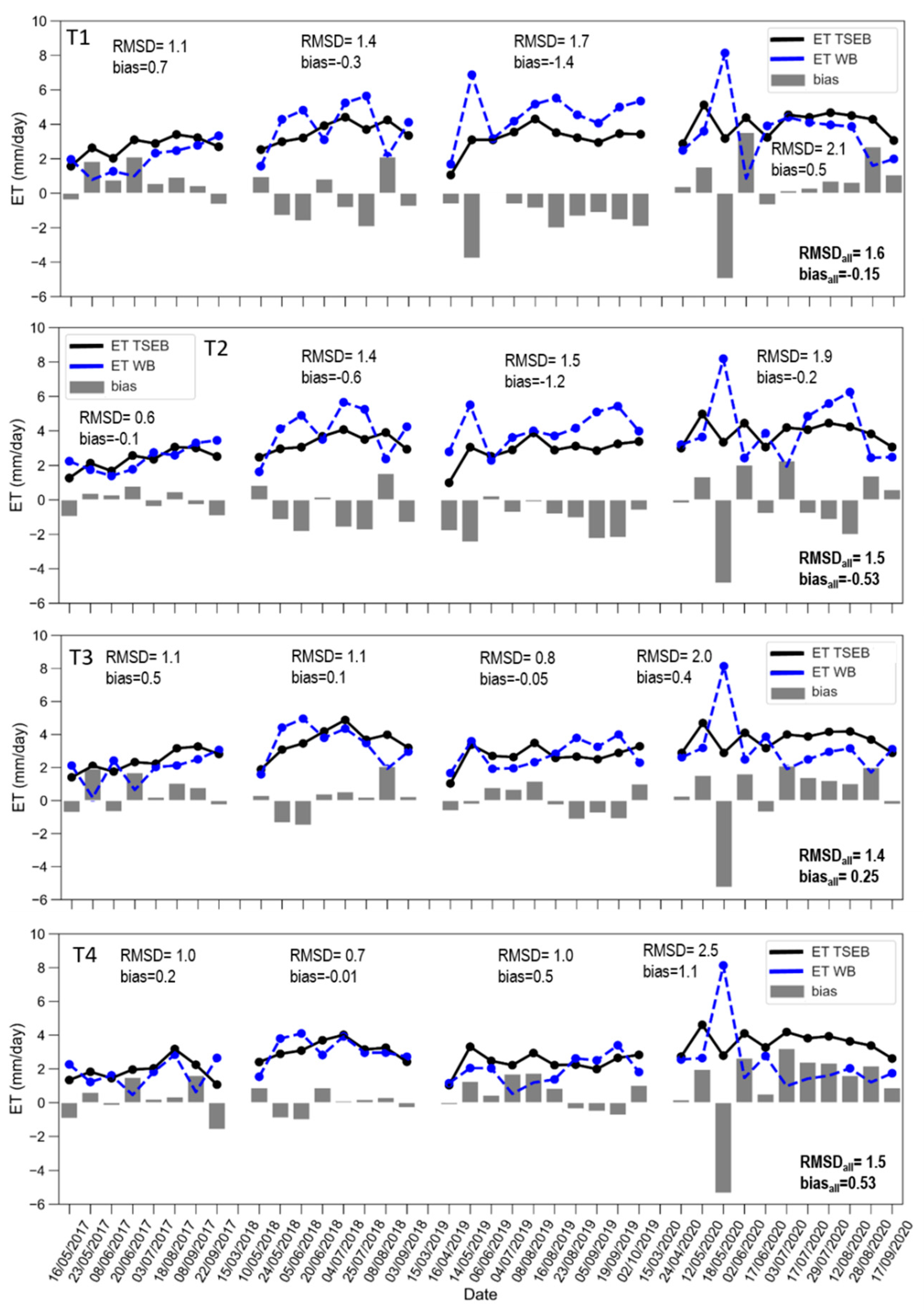
3.4. Comparison of ETa Estimates with TSEBS2+S3 and a Soil Water Balance Approach

While the eddy covariance footprint represents an integrated measurement of the energy fluxes from all four treatments, a way to assess the ETa estimates with TSEBS2+S3 for each individual irrigation treatment, ranging from stressed to well-watered conditions, is through an intercomparison with a soil water balance model. This was obtained for weekly or bi-weekly periods, on the basis of soil water content reads with a neutron probe.
A scatter plot encompassing all ETa data obtained through the water balance and estimated with the TSEBS2+S3 approaches showed an average seasonal root mean square deviation (RMSD) and bias of 1.54 and −0.02 mm/day, respectively (Figure 9a). Results did not show significant differences between irrigation treatments. Although the joint data analysis does not show good results, when this was analyzed individually for each irrigation treatment and year, the time series of both methodologies followed the same trend throughout the growing seasons (Figure 10). The largest sources of error came from longer periods between neutron probe measurements and due to precipitation events. The RMSD ranged from 0.6 to 2.5 mm/day, but when the periods with precipitation events corresponding to 15 May 2019 and 18 May 2020 were not considered, maximum RMSD dropped to 2.0 mm/day. Similarly, average seasonal RMSD decreased to 1.19 mm/day when removing these dates (Figure 9b). In both approaches, a clear increase can be observed in ETa from 2017 to 2020. RMSD and bias were higher in 2020, when seasonal cumulative ETa reached its maximum values. For that year, ETa TSEBS2+S3 values for T3 and T4 were significantly higher than those obtained with ETa WB, suggesting a slight overestimation in periods of severe water stress. However, this cannot be confirmed in this study since T4 trees were also stressed in 2018 and 2019 and this overestimation was not observed.

4. Discussion

4.1. Validation of Energy Fluxes

The imbalance between Rn-G and LE+H represents the non-closure of the surface energy balance which might be attributable to differences between the sampling frequencies or the footprint measurements. Moreover, other energy sources or sinks are not considered in these energy fluxes, such as canopy storage [77]. In another context, flux uncertainties may indicate an underperformance of TSEB since typical low errors for sensible heat flux (H) usually fluctuate around 50 W/m2 and the ones obtained in this study are slightly higher. However, the footprint of the present study had a high degree of heterogeneity due to differences in almond water status and vegetative growth. This makes these results harder to compare with those from other studies in which fluxes are usually measured in well-irrigated homogeneous fields. Despite this, Guzinsky et al. [44] reported an error in H of 94 W/m2 in woody crops using the TSEB-PT approach. On the other hand, He et al. [34] evaluated the METRIC modelling approach using Landsat in an almond orchard and obtained an RMSE of approximately 75 W/m2 for LE. These results were not far from the RMSE of 90 and 80 W/m2 for H and of 87 and 108 W/m2 for LE observed in our study, respectively, for TSEBS2+S3 and TSEBLandsat.
The eddy covariance footprint may also vary from day to day. Although the main wind direction in the orchard was NW, it can vary throughout the day. In part, this could affect the measured fluxes according to the relative contribution of each treatment. On the other hand, the bias observed in Rn (−46 W/m2) may be related to the fact that the net radiometer is placed over a fully irrigated tree of T1, which means that it is above the highest and densest canopy in the orchard. Therefore, this bias is actually related to the canopy-intercepted radiation and therefore can lead to higher observed Rn values than those modelled with TSEB but as well in larger EC closure errors. It should also be noted that the inputs for the net radiation calculation are obtained from a 20 × 20 m pixel which integrates both bare soil and canopy. Observed overestimations in H may be related to horizontal advection of hot, dry air. During these days, temperatures were over 35 °C, and the surrounding bare soil can heat up this air, provoking such conditions. These advective conditions can significantly increase the localized evaporative demand over an irrigated field, deriving larger latent heat fluxes. In such cases, the additional energy required for evaporation is extracted from the surface itself, resulting in negative sensible heat, increased closure errors [78] and more difficulties of TSEB-PT in accurately estimating sensible heat flux [79].
Orchards often present highly clumped canopies and therefore a significant area of the ground has no or very little leaf biomass. This causes distinct wind attenuation towards the soil surface, with larger attenuation within the canopy and lower in-ground exposed areas. This issue alters the momentum, heat and vapor exchange in the soil-plant-atmosphere continuum [80]. It has been proven that using wind profile models adapted to vertically heterogeneous canopies can improve the accuracy of surface energy flux estimations [81,82] compared to other profiles designed for homogeneous canopies [83]. However, these wind attenuation profile models require additional parameters related to the canopy structure that may not always be available, in particular for operational and large-scale applications such as regional water accounting with satellite imagery [46].
Landsat-8 was also used to analyze how the sharpening technique applied to Sentinel imagery can influence the flux estimations under water stress conditions. However, results from Figure 5 showed that flux from the sharpened S2+S3 LST were not significantly different from those of the lone Landsat 8 LST. An even higher-resolution sensor may be required for this study site, mainly because the 100 m resolution TIR on board Landsat-8 might not be enough to acquire representative LST pixels per plot. In fact, data from the Ecosystem Spaceborne Thermal Radiometer Experiment on Space Station (ECOSTRESS), using the International Space Station (ISS) [41], were also evaluated for the present study, but the lack of valid observations made this comparison unviable and it was therefore not presented in this article.

4.2. Land Surface Temperature (LST) and Biophysical Parameters of the Vegetation

The DMS approach used in this study to sharpen low-resolution LST with high-resolution shortwave data is based on the assumption that there exists a statistical relation between the two spectral regions. The decision tree machine learning algorithm used allows a high level of complexity in non-linear relations between the shortwave reflectance bands and the LST [45]. However, there is some controversy about the accuracy of high-resolution LST estimates using this approach in highly variable landscapes, where there is an interaction between different land uses (e.g., rainfed and irrigated fields), an agricultural-to-urban landscape continuum, or in cases where crops are stressed but there is no reduction in biomass [47]. Until the launch of higher-resolution LST missions, the use of data sharpening methods is necessary. Some other machine learning ensemble algorithms exist which have also demonstrated high accuracy in downscaling LST and, at the same time, less overfitting. For instance, a decision-tree-based ensemble machine learning algorithm that uses a gradient boosting framework (XGBoost) has recently become popular mainly due to its high accuracy and ease of implementation [84,85]. However, the computation time can be high when scaling it to a bigger dataset or a high number of variables. Other approaches based on use of a light gradient boosting machine (LightGBM) [86] have reported similar accuracy to that of XGBoost but with lower computation time. Adoption of such approaches could probably improve the accuracy of LST estimates. Although there were no in situ measurements to validate actual sharpened LST, a spatiotemporal pattern in LST was clearly observed between treatments (Figure 6 and Figure 11), with T4 showing significantly higher LST values during 2019 and 2020. Since sharpened LST was obtained from machine learning algorithms which relate S3 LST with S2 shortwave bands at coarse resolutions, it is probable that differences in sharpened LST between irrigation treatments can mainly be attributed to differences in vegetative growth variables. This has previously been observed in grapevines by Bellvert et al. [47], who reported that sharpened LST for severely stressed vines tends to be underestimated, especially if there is no evidence of a decrease in biomass.
Radiative transfer models for retrieving biophysical parameters are already being operationally produced and integrated into models for decision making [60]. Among them, LAI is one of the main drivers needed in TSEB. Burchard-Levine [87] demonstrated that a change of 0.1 in LAI is associated with a 2.9% change in simulated H with TSEB. However, the retrieval of accurate LAI and canopy structure estimates, especially in heterogeneous row crops, continues to be a major challenge. Nonetheless, the current study was able to detect spatiotemporal differences in LAI and FVC between irrigation treatments (Figure 6 and Figure 11).
It is worth noting that several assumptions are taken into account when predicting the biophysical parameters of vegetation from Sentinel-2, most importantly that the radiative transfer model that is used assumes horizontally and vertically homogeneous vegetation. Therefore, in orchards and row crops or in transition zones between different vegetation patches, inversion of this RTM may yield larger uncertainty. Moreover, any retrieval algorithm is susceptible to satellite signal uncertainty due to geometric misregistration, anisotropic reflectance effects, electronic errors, artifacts due to data resampling, atmosphere and clouds [88]. In those cases, noisy retrievals can be observed, such as unexpected peaks inherent to the vegetation phenology or other external factors such as pruning or other agronomic practices that may affect vegetation vigor. For this reason, in the present study, the biophysical parameters were filtered using a Savitzky–Golay filter, which smoothed the temporal series without losing the actual information [89]. Another assumption to be considered is that biophysical retrievals may be affected by cover crop in the interrow, especially at the beginning of each growing season. In this study, an increase in LAI was observed at the beginning of each growing season (until late June), probably attributable to grass and weeds growing in the interrow. This effect cannot be separated from a single-view satellite observation (for the S2 tile T31TBF, the VZA is 2.28 degrees in the study site). Three-dimensional RTM models, such as FLIGHT [90] or DART-3D [91], where the simulated scenes can include heterogeneous canopy structures based on plant architecture and other aspects such as weeds in the interrow, may be required for retrieving biophysical parameters in sparse woody crops. It would be interesting to explore the use of these models in future works since more efficient solutions have recently been implemented. For example, DART-3D applied an unbiased bidirectional path tracing method called DART-Lux, which can be a hundred times more efficient than the previous version [92]. However, the greater the complexity of the model, the lower the suitability of its inversion, as it could lead to many likely solutions even when different inputs are used.

4.3. Seasonal Actual Evapotranspiration (ETa)

For many years, different studies have shown the feasibility of using different SEB models to estimate energy fluxes in different crops, using data from different satellites. In general, satellite-derived energy fluxes have been validated with eddy covariance or surface renewal instrumentation [8,46,78,93]. Common to most of these studies is that fluxes are assessed temporarily during one or several growing seasons, and the spatial variability in terms of the crop’s vegetative growth or water status of energy fluxes within the footprint is low. Moreover, from our knowledge, no study has assessed ETa estimates through surface energy models such as the TSEBS2+S3 in heterogeneous row crops irrigated at different levels, thus forcing eventual differences in water status.
This study demonstrates the usefulness of the TSEBS2+S3 approach to assess ETa in an almond orchard with a high degree of spatial variability in terms of water status. The seasonal average RMSD ranged from 1.4 to 1.6 mm/day and the bias from −0.53 to 0.53 mm/day in comparison to the water balance approach, showing similar values for all irrigation treatments.
The maximum cumulative ETa values obtained in this study for each specific year ranged from 760 to 915 mm, corresponding with a maximum FVC of 40% and 61%, respectively. These seasonal values were comparable with other studies also conducted in a semi-arid Mediterranean climate. For instance, Lopez-Lopez et al. [9] reported an annual ETa ranging from 923 to 1220 mm in fully irrigated almond trees with an FVC of 58 and 75%, respectively. The same study reported an average seasonal ETa of 699 mm for stressed almonds, which on average corresponded to 36% less in comparison to the fully irrigated ones. In our study, maximum differences in ETa between stressed (T4) and well-watered almonds (T1) were observed in 2019 and were as high as 20%. Similarly, Stevens et al. [20] observed a cumulative ETa of 1257 mm in almond trees with an FVC of 65%. In this case, however, the seasonal ET0 (ET0 = 1365 mm) and the total sums of irrigation and precipitation (I + P = 1409 mm) were higher than in our study. Goldhamer and Fereres [7] also estimated similar seasonal ETa values in almond trees with an average FVC of 80% and under ten irrigation levels, which ranged from 1100 to 1350 mm (ET0 = 1170 mm). In these studies, calculations of ETa were obtained through a water balance approach, where soil water content was either monitored with neutron probe measurements or time domain reflectometry (TDR) sensors. Since neutron probe measurements are scarce in space and time, mainly because measurements are performed manually and a certified person is needed, measurements cannot be carried out periodically. Likewise, installing TDR sensors may not be an appropriate methodology due to the large number of sensors required to characterize total soil water content within tree spacing distance. For both reasons, commonly used soil water balance approaches may have some error in accounting for ETa. Studies such as that of Bellvert et al. [8], which assessed seasonal ETa on the basis of eddy covariance or surface renewal instrumentation, also reported annual water consumption of 1194.8 mm for a dense (80% FVC) high canopy of mature almonds. In Figure 11, we plotted average FVC with cumulated ETa and crop coefficients (Kc) only for those treatments that were transpiring at potential rates (T1 and T2) and were compared with those of T4 as well as with data from other available studies. Since the almond trees of our study were planted in 2016, the maximum average FVC values were only 50% in 2020, which corresponded with a seasonal ETa of 900 mm. The regression follows an exponential model and clearly fits already existing datasets. As most of the current available studies were conducted in mature almond trees with an FVC > 60%, the combination of the available datasets with the results obtained in the current study in young almond trees allowed completion of the regression. It is also interesting to see that despite the fact that T4 received less water and transpired significantly less during the last three years of study, points followed the same trend as other treatments. Therefore, the lower ETa observed in T4 was basically explained by trees being smaller.
Finally, a spatial pattern was also observed for the biophysical parameters LST and ETa, with differences observable between irrigation treatments. On average, maximum differences in FVC and LAI between treatments were observed during the last two years of the experiment (Figure 12a). The highest spatial variability in ETa was also observed in 2019 and 2020. Figure 12b shows in more detail the spatial variability of LST, LAI and daily ETa for three representative dates along the growing season. This figure also represents the spatial resolution with respect to the plots. It can be observed that only one or two pixels fall entirely into each treatment. LST at the beginning of the season was around 295K in contrast with mid-July LST where the soil can be up to 320K or even higher in bare areas. LAI differences were also lower at the beginning of the season and became higher at mid-summer and at the end of the season. ETa peak was at mid-summer 2020, reaching around 5 mm/day in T1.

5. Conclusions

The Copernicus program provides a wide range of services and datasets with capabilities that can be used for several operational agricultural applications. For irrigation management, however, a high-resolution TIR sensor is still a missing feature for operational estimates of crop evapotranspiration. Consequently, while waiting for the launch of higher-resolution LST missions, the use of modern data fusion techniques is required to compensate for the current lack of high-resolution TIR observations. This study demonstrates that use of the TSEB model with sharpened Sentinel-2 and Sentinel-3 imagery is suitable to monitor water use in almond trees irrigated under different water regimes. Sensible heat flux showed an RMSD of 90 W/m2, LE of 87 W/m2, and G an error of 37 W/m2. The assessed Sentinel-2 biophysical parameters such as LAI and FVC were able to distinguish differences in vegetative growth between irrigation treatments. Moreover, sharpened LST showed significant differences between the most extreme irrigation treatments (T1 and T4) during the last two years of the study period. The comparison of ETa with the soil water balance model showed an RMSD ranging from 0.6 to 2.5 mm/day. The maximum differences in cumulative ETa between irrigation treatments were obtained in 2019, amounting to between 20% and 13% less when comparing T1 and T4.

Author Contributions

Experimental design, J.G.; conceptualization, C.J.-Č., J.B., J.G. and H.N.; methodology, C.J.-Č.; software, H.N., C.J.-Č. and M.P.-S.; validation, C.J.-Č. and J.B.; formal analysis, C.J.-Č. and J.B.; investigation, C.J.-Č., J.B. and H.N.; data curation, C.J.-Č., M.P.-S. and J.B.; writing—original draft preparation, C.J.-Č. and J.B.; writing—review and editing, C.J.-Č., J.B., J.G., M.P.-S. and H.N. All authors have read and agreed to the published version of the manuscript.

Funding

This research was partially supported by the following three projects: MOIST (Managing and Optimizing Irrigation by Satellite Tools) (No. 7049-00004A) funded by the Innovations Fund Denmark, PRIMA ALTOS (No. PCI2019-103649) and IRRINTEGRAL (No. RTI2018-099949-R-C21) funded by the Ministry of Science, Innovation and Universities of the Spanish government.

Data Availability Statement

Not applicable.

Acknowledgments

The authors would also like to thank all the Efficient Use of Water in Agriculture program team, at the IRTA, for their technical support, the “Diputació de Lleida” for allowing us to conduct this study in the almond orchard experimental station, as well as the Horizon 2020 Programme for Research and Innovation (H2020) of the European Commission, in the context of the Marie Sklodowska-Curie Research and Innovation Staff Exchange (RISE) action and ACCWA project: grant agreement No.: 823965.

Conflicts of Interest

The authors declare no conflict of interest.

References

  1. FAOSTAT. FAO Statistical Database. 2018. Available online: http://www.fao.org/faostat/en/#data/QC (accessed on 13 October 2021).
  2. MAPA. Ministerio de Agricultura, Pesca y Alimentación. 2020. Available online: https://www.mapa.gob.es/es/estadistica/temas/estadisticas-agrarias/agricultura/superficies-producciones-anuales-cultivos/ (accessed on 10 September 2021).
  3. Egea, G.; Nortes, P.; González-Real, M.M.; Baille, A.; Domingo, R. Agronomic response, and water productivity of almond trees under contrasted deficit irrigation regimes. Agric. Water Manag. 2010, 97, 171–181. [Google Scholar] [CrossRef]
  4. López-López, M.; Espadafor, M.; Testi, L.; Lorite, I.; Orgaz, F.; Fereres, E. Water requirements of mature almond trees in response to atmospheric demand. Irrig. Sci. 2018, 36, 271–280. [Google Scholar] [CrossRef]
  5. Moldero, D.; López-Bernal, Á.; Testi, L.; Lorite, I.; Fereres, E.; Orgaz, F. Long-term almond yield response to deficit irrigation. Irrig. Sci. 2021, 39, 409–420. [Google Scholar] [CrossRef]
  6. Spinelli, G.M.; Snyder, R.L.; Sanden, B.L.; Shackel, K.A. Water stress causes stomatal closure but does not reduce canopy evapotranspiration in almond. Agric. Water Manag. 2016, 168, 11–22. [Google Scholar] [CrossRef]
  7. Goldhamer, D.A.; Fereres, E. Establishing an almond water production function for California using long-term yield response to variable irrigation. Irrig. Sci. 2017, 35, 169–179. [Google Scholar] [CrossRef]
  8. Bellvert, J.; Adeline, K.; Baram, S.; Pierce, L.; Sanden, B.L.; Smart, D.R. Monitoring Crop Evapotranspiration and Crop Coefficients over an Almond and Pistachio Orchard Throughout Remote Sensing. Remote Sens. 2018, 10, 2001. [Google Scholar] [CrossRef] [Green Version]
  9. López-López, M.; Espadafor, M.; Testi, L.; Lorite, I.J.; Orgaz, F.; Fereres, E. Yield response of almond trees to transpiration déficits. Irrig. Sci. 2018, 36, 111–120. [Google Scholar] [CrossRef]
  10. Confederación Hidrográfica del Guadalquivir (CHG). Plan Hidrológico de la Demarcación del Guadalquivir 2015–2021, R.D. 1/2016; Confederación Hidrográfica del Guadalquivir: Sevilla, Spain, 2016. [Google Scholar]
  11. Fereres, E.; Soriano, M.A. Deficit irrigation for reducing agricultural water use. J. Exp. Bot. 2007, 58, 147–159. [Google Scholar] [CrossRef] [Green Version]
  12. Expósito, A.; Berbel, J. The economics of irrigation in almond orchards. Application to southern Spain. Agronomy 2020, 10, 796. [Google Scholar] [CrossRef]
  13. Goldhamer, D.A.; Viveros, M. Effects of preharvest irrigation cutoff durations and postharvest water deprivation on almond tree performance. Irrig. Sci. 2000, 19, 125–131. [Google Scholar] [CrossRef]
  14. Esparza, G.; DeJong, T.M.; Weinbaum, S.A.; Klein, I. Effects of irrigation deprivation during the harvest period on yield determinants in mature almond trees. Tree Physiol. 2001, 21, 1073–1079. [Google Scholar] [CrossRef] [PubMed]
  15. Girona, J.; Mata, M.; Marsal. Regulated deficit irrigation during the kernel-filling period and optimal irrigation rates in almond. Agric. Water Manag. 2005, 75, 152–167. [Google Scholar] [CrossRef]
  16. Allen, R.G.; Pereira, L.S.; Raes, D.; Smith, M. Crop Evapotranspiration. Guidelines for Computing Crop Water Requirements; FAO Irrigation and Drainage Paper 56; FAO: Rome, Italy, 1998; 300p. [Google Scholar]
  17. Allen, R.G.; Pereira, L.S. Estimating crop coefficients from fraction of ground cover and height. Irrig. Sci. 2009, 28, 17–34. [Google Scholar] [CrossRef] [Green Version]
  18. García-Tejero, I.F.; Hernández, A.; Rodríguez, V.M.; Ponce, J.R.; Ramos, V.; Muriel, J.L.; Durán-Zauzo, V.H. Estimating almond crop coefficients and physiological response to water stress in semiarid environments (SW Spain). J. Agric. Sci. Technol. 2015, 17, 1255–1266. [Google Scholar]
  19. Espadafor, M.; Orgaz, F.R.; Testi, L.; Lorite, I.J.; Villalobos, F.J. Transpiration of Young almond trees in relation to intercepted radiation. Irrig. Sci. 2015, 33, 265–275. [Google Scholar] [CrossRef] [Green Version]
  20. Stevens, R.M.; Ewenz, C.M.; Grigson, G.; Conner, S.M. Water use by an irrigated almond orchard. Irrig. Sci. 2012, 30, 189–200. [Google Scholar]
  21. Girona, J.; del Campo, J.; Mata, M.; Lopez, G.; Marsal, J.A. comparative study of apple and pear tree water consumption measured with two weighing lyismeters. Irrig. Sci. 2011, 29, 55–63. [Google Scholar] [CrossRef]
  22. Er-Raki, S.; Chehbouni, A.; Ezzahar, J.; Khabba, S.; Boulet, G.; Hanich, L.; Williams, D. Evapotranspiration Partitioning from Sap Flow and Eddy Covariance Techniques for Olive Orchards in Semi-Arid Region. Acta Hortic. 2009, 846, 201–208. [Google Scholar] [CrossRef]
  23. Testi, L.; Villalobos, F.J.; Orgaz, F. Evapotranspiration of a young irrigated olive orchard in southern Spain. Agric. Meteorol. 2004, 121, 1–18. [Google Scholar] [CrossRef]
  24. Ferreira, M.I. Stress Coefficients for Soil Water Balance Combined with Water Stress Indicators for Irrigation Scheduling of Woody Crops. Horticulturae 2017, 3, 38. [Google Scholar] [CrossRef] [Green Version]
  25. Garnier, E.; Berger, A.; Rambal, S. Water balance and pattern of soil water uptake in a peach orchard. Agric. Water Manag. 1986, 11, 145–158. [Google Scholar] [CrossRef]
  26. Ahumada, L.; Ortega-Farias, S.; Poblete-Echevarría, C.; Peter, S. Estimation of stomatal conductance and stem water potential threshold values for water stress in olive trees (cv. Arbequina). Irrig. Sci. 2019, 37, 461–467. [Google Scholar] [CrossRef]
  27. Domínguez-Niño, J.M.; Oliver-Manera, J.; Girona, J.; Casadesús, J. Differential irrigation scheduling by an automated algorithm of water balance tuned by capacitance-type soil moisture sensors. Agric. Water Manag. 2020, 228, 105880. [Google Scholar] [CrossRef]
  28. Bastiaanssen, W.G.M.; Menenti, M.; Feddes, R.A.; Holtslag, A.A.M. A remote sensing surface energy balance algorithm for land (SEBAL). 1. Formulation. J. Hydrol. 1998, 212–213, 198–212. [Google Scholar] [CrossRef]
  29. Allen, R.G.; Tasumi, M.; Trezza, R. Satellite-based energy balance for mapping evapotranspiration with internalized calibration (METRIC)—Model. J. Irrig. Drain. Eng.-Asce 2007, 133, 380–394. [Google Scholar] [CrossRef]
  30. Norman, J.M.; Kustas, W.; Humes, K. A two-source approach for estimating soil and vegetation energy fluxes from observations of directional radiometric surface temperature. Agric. For. Meteorol. 1995, 77, 263–293. [Google Scholar] [CrossRef]
  31. Norman, J.M.; Kustas, W.P.; Prueger, J.H.; Diak, G.R. Surface flux estimation using radiometric temperature: A dual-temperature-difference method to minimize measurement errors. Water Resour. Res. 2000, 36, 2263. [Google Scholar] [CrossRef] [Green Version]
  32. Anderson, M.C.; Norman, J.M.; Mecikalski, J.R.; Torn, R.D.; Kustas, W.P.; Basara, J.B. A multiscale remote sensing model for disaggregating regional fluxes to micrometeorological scales. J. Hydrometeorol. 2004, 5, 343–363. [Google Scholar] [CrossRef]
  33. Boulet, G.; Mougenot, B.; Lhomme, J.-P.; Fanise, P.; Lili-Chabaane, Z.; Olioso, A.; Bahir, M.; Rivalland, V.; Jarlan, L.; Merlin, O.; et al. The SPARSE model for the prediction of water stress and evapotranspiration components from thermal infra-red data and its evaluation over irrigated and rainfed wheat. Hydrol. Earth Syst. Sci. 2015, 19, 4653–4672. [Google Scholar] [CrossRef] [Green Version]
  34. He, R.; Jin, Y.; Kandelous, M.M.; Zaccaria, D.; Sanden, B.L.; Snyder, R.L.; Jiang, J.; Hopmans, J.W. Evapotranspiration estimate over an almond orchard using Landsat satellite observations. Remote Sens. 2017, 9, 436. [Google Scholar] [CrossRef] [Green Version]
  35. Xue, J.; Bali, K.M.; Light, S.; Hessels, T.; Kisekka, I. Evaluation of remote sensing-based evapotranspiration models against surface renewal in almonds, tomatoes and maize. Agric. Water Manag. 2020, 238, 106228. [Google Scholar] [CrossRef]
  36. Anderson, M.C.; Allen, R.G.; Morse, A.; Kustas, W.P. Use of Landsat thermal imagery in monitoring evapotranspiration and managing water resources. Remote Sens. Environ. 2012, 122, 50–65. [Google Scholar] [CrossRef]
  37. Senay, G.B.; Friedrichs, M.; Singh, R.K.; Velpuri, N.M. Evaluating landsat 8 evapotranspiration for water use mapping in the Colorado River Basin. Remote Sens. Environ. 2016, 185, 171–185. [Google Scholar] [CrossRef] [Green Version]
  38. Semmens, K.A.; Anderson, M.C.; Kustas, W.P.; Gao, F.; Alfieri, J.G.; McKee, L.; Prueger, J.H.; Hain, C.R.; Cammalleri, C.; Yang, Y.; et al. Monitoring daily evapotranspiration over two California vineyards using Landsat 8 in a multi-sensor data fusion approach. Remote Sens. Environ. 2016, 185, 155–170. [Google Scholar] [CrossRef] [Green Version]
  39. Knipper, K.R.; Kustas, W.P.; Anderson, M.C.; Alfieri, J.G.; Prueger, J.H.; Hain, C.R.; Gao, F.; Yang, Y.; McKee, L.G.; Nieto, H.; et al. Evapotranspiration estimates derived using thermal-based satellite remote sensing and data fusion for irrigation management in California vineyards. Irrig. Sci. 2019, 37, 431–449. [Google Scholar] [CrossRef]
  40. Knipper, K.R.; Kustas, W.P.; Anderson, M.C.; Nieto, H.; Alfieri, J.; Prueger, J.; Hain, C.; Gao, F.; McKee, L.; Alsina, M.M.; et al. Using high-spatiotemporal thermal satellite ET retrievals to monitor water use over California vineyards of different climate, vine variety and trellis design. Agric. Water Manag. 2020, 241, 106361. [Google Scholar] [CrossRef]
  41. Fisher, J.B.; Lee, B.; Purdy, A.J.; Halverson, G.H.; Dohlen, M.B.; Cawse-Nicholson, K.; Wang, A.; Anderson, R.G.; Aragon, B.; Arain, M.A.; et al. ECOSTRESS: NASA’s Next GenerationMission to measure evapotranspirationfrom the International Space Station. Water Resour. Res. 2020, 56, e2019WR026058. [Google Scholar] [CrossRef]
  42. Anderson, M.C.; Yang, Y.; Xue, J.; Knipper, K.R.; Yang, Y.; Gao, F.; Hain, C.R.; Kustas, W.P.; Cawse-Nicholson, K.; Hulley, G.; et al. Interoperability of ECOSTRESS and Landsat for mapping evapotranspiration time series at sub-field scales. Remote Sens. Environ. 2021, 252, 112189. [Google Scholar] [CrossRef]
  43. Guzinski, R.; Nieto, H. Evaluating the feasibility of using Sentinel-2 and Sentinel-3 satellites for high-resolution evapotranspiration estimations. Remote Sens. Environ. 2019, 221, 157–172. [Google Scholar] [CrossRef]
  44. Guzinski, R.; Nieto, H.; Sandholt, I.; Karamitilios, G. Modelling High-Resolution Actual Evapotranspiration through Sentinel-2 and Sentinel-3 Data Fusion. Remote Sens. 2020, 12, 1433. [Google Scholar] [CrossRef]
  45. Gao, F.; Kustas, W.P.; Anderson, M.C. A data mining approach for sharpening thermal satellite imagery over land. Remote Sens. 2012, 4, 3287–3319. [Google Scholar] [CrossRef] [Green Version]
  46. Guzinski, R.; Nieto, H.; Sánchez, J.M.; López-Urrea, R.; Boujnah, D.M.; Boulet, G. Utility of Copernicus-Based Inputs for Actual Evapotranspiration Modeling in Support of Sustainable Water Use in Agriculture. IEEE J. Sel. Top. Appl. Earth Obs. Remote Sens. 2021, 14, 11466–11484. [Google Scholar] [CrossRef]
  47. Bellvert, J.; Jofre-Ĉekalović, C.; Pelechá, A.; Mata, M.; Nieto, H. Feasibility of Using the Two-Source Energy Balance Model (TSEB) with Sentinel-2 and Sentinel-3 Images to Analyze the Spatio-Temporal Variability of Vine Water Status in a Vineyard. Remote Sens. 2020, 12, 2299. [Google Scholar] [CrossRef]
  48. BOE. Real decreto 1201/2002, de 20 de Noviembre, por el que se Regula la Producción Integrada de Productos Agrícolas. Madrid: Boletin Oficial del Estado. 2002. Available online: https://www.boe.es/buscar/doc.php?id=BOE-A-2002-23340 (accessed on 25 April 2022).
  49. Goldhamer, D.A.; Girona, J. Crop yield response to water: Almond. In FAO Irrigation and Drainage; Steduto, P., Hsiao, T.C., Fereres, E., Raes, D., Eds.; Food and Agriculture Organization of the United Nations: Rome, Italy, 2012; Volume 66, pp. 358–373. [Google Scholar]
  50. Fereres, E. Drip Irrigation Management; Leaflet No. 21259; Cooperative Ext., Univ.: Berkeley, CA, USA, 1981. [Google Scholar]
  51. Kustas, W.P.; Norman, J.M. Evaluation of soil and vegetation heat flux predictions using a simple two-source model with radiometric temperatures for partial canopy cover. Agric. For. Meteorol. 1999, 94, 13–29. [Google Scholar] [CrossRef]
  52. Choudhury, B.J.; Idso, S.B.; Reginato, R.J. Analysis of an empirical model for soil heat flux under a growing wheat crop for estimating evaporation by an infrared-temperature based energy balance equation. Agric. For. Meteorol. 1987, 38, 283–297. [Google Scholar] [CrossRef]
  53. Santanello, J.A.; Friedl, M. Diurnal covariation in soil heat flux and net radiation. J. Appl. Meteorol. 2003, 42, 851–862. [Google Scholar] [CrossRef]
  54. McNaughton, K.G.; van den Hurk, B.J.J.M. A Lagrangian revision of the resistors in the 2-layer model for calculation the energy budget of a plant canopy. Bound.-Layer Meteor. 1995, 74, 261–288. [Google Scholar] [CrossRef]
  55. Choudhury, B.; Monteith, J. A four-layer model for the heat budget of homogeneous land surfaces. Q. J. R. Meteorol. Soc. 1988, 114, 373–398. [Google Scholar] [CrossRef]
  56. Kustas, W.P.; Nieto, H.; Morillas, L.; Anderson, M.C.; Alfieri, J.G.; Hipps, L.E.; Villagarcía, L.; Domingo, F.; Garcia, M. Revisiting the paper Using radiometric Surface temperature for Surface energy flux estimation in Mediterranean drylands from a two-source perspective. Remote Sens. Environ. 2016, 184, 645–653. [Google Scholar] [CrossRef] [Green Version]
  57. Kustas, W.; Anderson, M. Advances in thermal infrared remote sensing for land surface modeling. Agric. For. Meteorol. 2009, 149, 2071–2081. [Google Scholar] [CrossRef]
  58. Priestley, C.H.B.; Taylor, R.J. On the Assessment of Surface Heat Flux and Evaporation Using Large-Scale Parameters. Mon. Weather. Rev. 1972, 100, 81–92. [Google Scholar] [CrossRef]
  59. Weiss, M.; Baret, F. S2ToolBox Level 2 products: LAI, FAPAR, FCOVER—Version 1.1. Sentin. ToolBox Level2 Prod. 2016, 53. Available online: https://step.esa.int/docs/extra/ATBD_S2ToolBox_L2B_V1.1.pdf (accessed on 19 May 2021).
  60. Jacquemoud, S.; Verhoef, W.; Baret, F.; Bacour, C.; Zarco-Tejada, P.J.; Asner, G.P.; François, C.; Ustin, S.L. PROSPECT+SAIL models: A review of use for vegetation characterization. Remote Sens. Environ. 2009, 113, S56–S66. [Google Scholar] [CrossRef]
  61. Verhoef, W. Light scattering by leaf layers with application to canopy reflectance modeling: The SAIL model. Remote Sens. Environ. 1984, 16, 125–141. [Google Scholar] [CrossRef] [Green Version]
  62. Campbell, G.S.; Norman, J.M. An Introduction to Environmental Biophysics; Springer: New York, NY, USA, 1998. [Google Scholar]
  63. Savitzky, A.; Golay, M.J. Smoothing and differentiation of data by simplified least squares procedures. Anal. Chem. 1964, 36, 1627–1639. [Google Scholar] [CrossRef]
  64. Agam, N.; Kustas, W.P.; Anderson, M.C.; Li, F.; Neale, C.M.U. A vegetation index based technique for spatial sharpening of thermal imagery. Remote Sens. Environ. 2007, 107, 545–558. [Google Scholar] [CrossRef]
  65. Kustas, W.P.; Norman, J.M.; Anderson, M.C.; French, A.N. Estimating subpixel surface temperatures and energy fluxes from the vegetation index-radiometric temperature relationship. Remote Sens. Environ. 2003, 85, 429–440. [Google Scholar] [CrossRef]
  66. Parry, C.K.; Nieto, H.; Guillevic, P.; Agam, N.; Kustas, W.P.; Alfieri, J.; McKee, L.; McElrone, A.J. An intercomparison of radiation partitioning models in vineyard canopies. Irrig. Sci. 2019, 37, 239–252. [Google Scholar] [CrossRef]
  67. Campbell, G.S. Extinction coefficients for radiation in plant canopies calculated using an ellipsoidal inclination angle Distribution. Agric. For. Meteorol. 1986, 36, 317–321. [Google Scholar] [CrossRef]
  68. Raupach, M.R. Simplified expressions for vegetation roughness length and zero-plane displacement as functions of canopy height and area index. Bound.-Layer Meteorol. 1994, 71, 211–216. [Google Scholar] [CrossRef]
  69. Cammalleri, C.; Anderson, M.C.; Kustas, W.P. Upscaling of evapotranspiration fluxes from instantaneous to daytime scales for thermal remote sensing applications. Hydrol. Earth Syst. Sci. 2014, 18, 1885–1894. [Google Scholar] [CrossRef] [Green Version]
  70. Foken, T.; Aubinet, M.; Finnigan, J.J.; Leclerc, M.Y.; Mauder, M.; Paw U, K.T. Results of a panel discussion about the energy balance closure correction for trace gases. Bull. Am. Meteorol. Soc. 2011, 92, 13–18. [Google Scholar] [CrossRef] [Green Version]
  71. Barr, A.G.; King, K.M.; Gillespie, T.J.; den Hartog, G.; Neumann, H.H. A comparison of Bowen ratio and eddy correlation sensible and latent heat flux measurements above deciduous forest. Bound.-Layer Meteorol. 1994, 71, 21–41. [Google Scholar] [CrossRef]
  72. Twine, T.E.; Kustas, W.P.; Norman, J.M.; Cook, D.R.; Houser, P.R.; Meyers, T.P.; Prueger, J.H.; Starks, P.J.; Wesely, M.L. Correcting eddy-covariance flux underestimates over a grassland. Agric. For. Meteorol. 2000, 103, 279–3000. [Google Scholar] [CrossRef] [Green Version]
  73. Kljun, N.; Calanca, P.; Rotach, M.W.; Schmid, H.P. A simple two-dimensional parameterisation for flux footprint prediction (FFP). Geosci. Model Dev. 2015, 8, 3695–3713. [Google Scholar] [CrossRef] [Green Version]
  74. Baldocchi, D.D.; Falge, E.; Gu, L.; Olson, R.; Hollinger, D.; Running, S.; Anthoni, P.; Bernhofer, C.; Davis, K.; Evans, R.; et al. FLUXNET: A new tool to study the temporal and spatial variability of ecosystem-scale carbon dioxide, water vapor and energy flux densities. Bull. Am. Meteorol. Soc. 2001, 82, 2415–2435. [Google Scholar] [CrossRef]
  75. Wilson, K.; Goldstein, A.; Falge, E.; Aubinet, M.; Baldocchi, D.; Berbigier, P.; Bernhofer, C.; Ceulemans, R.; Dolman, H.; Field, C.; et al. Energy balance closure at FLUXNET sites. Agric Meteorol. 2002, 113, 223–243. [Google Scholar] [CrossRef] [Green Version]
  76. Sánchez, J.M.; Simón, L.; González-Piqueras, J.; Montoya, F.; López-Urrea, R. Monitoring Crop Evapotranspiration and Transpiration/Evaporation Partitioning in a Drip-Irrigated Young Almond Orchard Applying a Two-Source Surface Energy Balance Model. Water 2021, 13, 2073. [Google Scholar] [CrossRef]
  77. Foken, T.; Wimmer, F.; Mauder, M.; Thomas, C.; Liebethal, C. Some aspects of the energy balance closure problem. Atmos. Chem. Phys. 2006, 6, 4395–4402. [Google Scholar] [CrossRef] [Green Version]
  78. Alfieri, J.G.; Kustas, W.P.; Prueger, J.H.; Hipps, L.E.; Evett, S.R.; Basara, J.B.; Neale, C.M.; French, A.N.; Colaizzi, P.; Agam, N.; et al. On the discrepancy between eddy covariance and lysimetry-based surface flux measurements under strongly advective conditions. Adv. Water Resour. 2012, 50, 62–78. [Google Scholar] [CrossRef] [Green Version]
  79. Kustas, W.P.; Nieto, H.; García-Tejera, O.; Bambach, N.; McElrone, A.J.; Gao, F.; Alfieri, J.G.; Hipps, L.E.; Prueger, J.H.; Torres-Rua, A.; et al. Impact of advection on two-source energy balance (TSEB) canopy transpiration parameterization for vineyards in the California Central Valley. Irrig. Sci. 2022. [Google Scholar] [CrossRef]
  80. Massman, W. A comparative study of some mathematical models of the mean wind structure and aerodynamic drag of plant canopies. Bound.-Lay. Meteorol. 1987, 40, 179–197. [Google Scholar] [CrossRef]
  81. Cammalleri, C.; Anderson, M.; Ciraolo, G.; D’Urso, G.; Kustas, W.P.; la Loggia, G.; Minacapilli, M. The impact of in-canopy wind profile formulations on heat flux estimation using the remote sensing-based two-source model for an open orchard canopy in southern Italy. Hydrol. Earth Syst. Sci. 2010, 7, 4687. [Google Scholar]
  82. Nieto, H.; Kustas, W.P.; Torres-Rúa, A.; Alfieri, J.G.; Gao, F.; Anderson, M.C.; White, W.A.; Song, L.; Alsina, M.; Prueger, J.H.; et al. Evaluation of TSEB turbulent fluxes using different methods for the retrieval of soil and canopy component temperatures from UAV thermal and multispectral imagery. Irrig. Sci. 2019, 37, 389–406. [Google Scholar] [CrossRef] [PubMed] [Green Version]
  83. Goudriaan, J. Crop Micrometeorology: A Simulation Study; Center Agricoltural Publications and Documentation, Wageningen Universitait: Wageningen, The Netherlands, 1977. [Google Scholar]
  84. Ghosh, A.; Joshi, P.K. Hyperspectral imagery for disaggregation of land surface temperature with selected regression algorithms over different land use land cover scenes. ISPRS J. Photogramm. Remote Sens. 2014, 96, 76–93. [Google Scholar] [CrossRef]
  85. Xu, S.; Zhao, Q.; Yin, K.; He, G.; Zhang, Z.; Wang, G.; Wen, M.; Zhang, N. Spatial Downscaling of Land Surface Temperature Based on a Multi-Factor Geographically Weighted Machine Learning Model. Remote Sens. 2021, 13, 1186. [Google Scholar] [CrossRef]
  86. Ke, G.; Meng, Q.; Finley, T.; Wang, T.; Chen, W.; Ma, W.; Ye, Q.; Liu., T.-Y. LightGMB: A high eficient gradient boosting decision tree. In Proceedings of the 31st Conference on Neural Information Processing Systems, Long Beach, CA, USA, 4–9 December 2017. [Google Scholar]
  87. Burchard-Levine, V.; Nieto, H.; Riaño, D.; Migliavacca, M.; El-Madany, T.S.; Perez-Priego, O.; Carrara, A.; Martín, M.P. Seasonal Adaptation of the Thermal-Based Two-Source Energy Balance Model for Estimating Evapotranspiration in a Semiarid Tree-Grass Ecosystem. Remote Sens. 2020, 12, 904. [Google Scholar] [CrossRef] [Green Version]
  88. Goward, S.N.; Markham, B.; Dye, D.G.; Dulaney, W.; Yang, J. Normalized difference vegetation index measurements from the advanced very high resolution radiometer. Remote Sens. Environ. 1991, 35, 257–277. [Google Scholar] [CrossRef]
  89. Cai, Z.; Jönsson, P.; Jin, H.; Eklundh, L. Performance of Smoothing Methods for Reconstructing NDVI Time-Series and Estimating Vegetation Phenology from MODIS Data. Remote Sens. 2017, 9, 1271. [Google Scholar] [CrossRef] [Green Version]
  90. North, P.R.J. Three-dimensional forest light interaction model using a Monte Carlo method. IEEE Trans. Geosci. Remote Sens. 1996, 34, 946–956. [Google Scholar] [CrossRef]
  91. Gastellu-Etchegorry, J.-P.; Demarez, V.; Pinel, V.; Zagolski, F. Modeling radiative transfer in heterogeneous 3-D vegetation canopies. Remote Sens. Environ. 1996, 58, 131–156. [Google Scholar] [CrossRef] [Green Version]
  92. Yingjie, W.; Gastellu-Etchegorry, J.-P. Accurate and Fast Simulation of Remote Sensing Images at Top of Atmosphere with Dart-lux. Remote Sens. Environ. 2021, 256, 112311. [Google Scholar]
  93. Gonzalez-Dugo, M.P.; Neale, C.M.U.; Mateos, L.; Kustas, W.P.; Prieger, J.H.; Anderson, M.C.; Li, F. A comparison of operational remote sensing-based models for estimating crop evapotranspiration. Agric. For. Meteorol. 2009, 149, 1843–1853. [Google Scholar] [CrossRef]
Figure 1. Study site of the almond orchard located in Maials (41°22.9′172″N, 0°31.27′619″E) (Lleida, Spain), showing in (a) the four S2 UTM tiles downloaded in this study, (b) the area of interest (AOI) where the biophysical parameters and ETa were processed and (c) detailed view of the experimental design, where each plot corresponds to different irrigation treatments (T1 to T4).
Remotesensing 14 02106 g001
Figure 3. Eddy covariance tower footprint for 21st July 2020, representing the fetch and the relative contribution for a typical day, at high resolution (left) and resampled at 20 m to match Sentinel-2 resolution (right). The overall spot represents an 80% contribution for both plots.
Remotesensing 14 02106 g003
Figure 4. Energy balance closure of sensible (H) and latent heat flux (LE) against net radiation (Rn) minus soil heat flux (G) in the almond orchard.
Remotesensing 14 02106 g004
Figure 5. Observed vs. modeled instantaneous energy balance fluxes for the TSEB model using sharpened LST from Sentinel-2 and Sentinel-3 (left) and TSEB with Landsat LST (right).
Remotesensing 14 02106 g005
Figure 6. Seasonal patterns of (a) leaf area index (LAI) and (b) fractional vegetation cover (FVC), estimated from the Sentinel-2 biophysical processor available in the SNAP software, and (c) sharpened land surface temperature (LST), for each irrigation treatment during the 2017–2020 growing seasons. Letters show Tukey’s HSD analysis for years with significant differences (p ≤ 0.05). Lines show the mean and the shading region shows the error bounds for the four plots within each irrigation treatment. * means significant differences at p ≤ 0.05, while n.s. means not statistically significant differences at p ≤ 0.05.
Remotesensing 14 02106 g006
Figure 7. Time series of actual crop evapotranspiration for each irrigation treatment estimated with the TSEBS2+S3 approach for the growing seasons 2017 to 2020. PP corresponds to precipitation. Lines show the mean values and the shading region shows the error bounds for the four plots within each irrigation treatment.
Remotesensing 14 02106 g007
Figure 8. Cumulative mean daily (a) actual crop evapotranspiration (ETa) and reference evapotranspiration (ET0) and (b) sum of precipitation and irrigation, for each irrigation treatment during the four growing seasons (2017–2020). Letters show Tukey’s HSD analysis for treatments with significant differences (p ≤ 0.05). Lines show the mean and the shading region shows the error bounds for the four plots within each irrigation treatment. * means significant differences at p ≤ 0.05, while n.s. means not statistically significant differences at p ≤ 0.05.
Remotesensing 14 02106 g008
Figure 9. Relationship between actual evapotranspiration (ETa) obtained with the TSEBS2+S3 approach and the soil water balance (WB) with (a) all data available and (b) the removal of dates with precipitation events and dates with two consecutive soil neutron measurements longer than 20 days.
Remotesensing 14 02106 g009
Figure 10. Comparison of actual evapotranspiration (ETa) obtained with the TSEBS2+S3 approach and a soil water balance (WB). Each treatment corresponds to one plot. RMSD is the root mean square deviation, and bias corresponds to the difference between modelled ETa.
Remotesensing 14 02106 g010
Figure 11. Relationship between mean fractional vegetation cover (FVC) and (a) cumulative actual crop evapotranspiration (ETa) and (b) seasonal mean crop coefficients (Kc) for each growing season. Values with symbols corresponded to well-watered treatments (T1 and T2), and in red circle was T4. x corresponds to the following references: [4,5,7,8,9,20,34].
Remotesensing 14 02106 g011
Figure 12. Spatial patterns of (a) mean leaf area index (LAI), fractional vegetation cover (FVC) and cumulative actual evapotranspiration (ETa; growing season March–October inclusive) for each year, and (b) land surface temperature (LST), leaf area index (LAI) and daily evapotranspiration for three specific dates in the last year of the experiment.
Remotesensing 14 02106 g012
Table 1. Different statistics between TSEBS2+S3 and TSEBLandsat flux outputs and EC observations.
TSEBs2+s3TSEBLandsat
RnHLEGRnHLEG
RMSE639087371038010843
MAE5473692992667638
Bias−46−439−7−92−12−42−32
% diff−8.2−20.13.7−6.5−15.1−5.8−15.9−24.1
NRMSE0.110.440.350.340.170.380.410.33
NMAE0.090.360.270.260.150.320.290.29
RMSE is root mean square error, MAE is the mean absolute error, Bias is the average value of the modelled fluxes–observed fluxes; % diff is the modelled fluxes–observed fluxes divided by the observed fluxes × 100, NRMSE and NMAE are the normalized RMSE and MAE, which respectively related the RMSE and MAE to the observed range of the variable.
Table 2. Reference evapotranspiration (ET0), precipitation and irrigation amounts within each growing season (1 March–30 November) for the four treatments and during the four years of the study.
VariableTreatment2017201820192020
ET0-1130.81029.91113.01039.3
Precipitation-226394224.0350.2
IrrigationT1313.2 a512.7 a730.7 a634.1 a
T2311.9 a521.6 a542.6 b573.3 b
T3307.74 a458.45 a413.3 c474.7 c
T4219.3 b319.0 b272.2 d284.2 d
Prob > F0.0002 *0.0001 *<0.0001 *<0.0001 *
* Different letters mean significant differences at p ≤ 0.05 using Tukey’s honest significant difference test.
Publisher’s Note: MDPI stays neutral with regard to jurisdictional claims in published maps and institutional affiliations.

