Real-Time Precise DGNSS/INS Integrated Relative Positioning with High Output Rate and Low Broadcast Rate for Kinematic-to-Kinematic Applications

Abstract

High-output-rate relative positions are required for high-speed safety-critical kinematic-to-kinematic applications such as pre-crash sensing and shipboard landing. We propose a real-time, high-output-rate relative positioning method based on the integration of a real time kinematic (RTK) differential global navigation satellite systems (DGNSS) relative positioning algorithm, carrier-phase-based tightly coupled GNSS/Inertial navigation system (TC-GNSS/INS) integration algorithm and polynomial prediction algorithm for position increment. We focus on the rarely studied issue that data broadcast rates and sampling rates have effects on the integrated relative positioning accuracy under different motion states of a moving base. A vehicle-to-vehicle field test with a frequently turning base demonstrates the advantages of the proposed method, such as low bit rate of broadcast data, high output rate of position solutions and excellent real-time tolerance of latency. The results show that compared with the 10-Hz output of sole RTK DGNSS relative positioning, the proposed method can provide centimeter-level-accuracy relative positions at an output rate of 125 Hz with a sampling rate of 1 Hz, and the bit rate can be reduced by 83.12%. A UAV-to-boat field test with straight-line-motion moving base is then carried out to validate the applicability of the proposed system for aircraft applications. The results show that the broadcast rate of position increments of the moving base can be further reduced.

1. Introduction

Nowadays, many safety-critical kinematic-to-kinematic applications require output rates of precise relative positions of 10 Hz to 50 Hz or more, such as vehicle-to-vehicle cooperative safety applications [1], automated air refueling and shipboard relative landing [2]. Automatic cruise control applications require an update rate of between 10 Hz and 20 Hz [3]. Cooperative vehicular applications such as lane-change, emergency brake lights and forward collision warnings require 10 Hz and the pre-crash sensing application even requires an output rate of up to 50 Hz [1]. High-speed applications such as autopilot and airborne positioning also require a sampling rate of GNSS data of 50 Hz [4].

Carrier-phase-based RTK DGNSS relative positioning technology is widely adopted in kinematic-to-kinematic applications to provide precise relative positioning such as vehicle-to-vehicle cooperative positioning [2,5], formation flight [6,7], collision detection between aircrafts [8] and shipboard landing [9,10]. Raw GNSS observations should be broadcast from a moving base to a rover by radio; the synchronized observations are required for relative positioning. With ambiguities correctly fixed, centimeter-level accuracy can be achieved [11,12,13]. As the raw GNSS observations need to be transmitted by wireless datalink, challenges such as nondeterministic latency, packet drops and bandwidth limitations cannot be avoided in real-time relative positioning [1]. Packet drops will increase latency. Even though modern receiver technology now enables sampling of GNSS observations at very high rates, such as 50 Hz or even higher [14,15], the huge data broadcast rate will bring heavy communication pressure and computational load. Much research has been done on high-rate output for relative positions [16,17,18,19,20,21]. Comstock [16] developed RTK positioning technology with a broadcast rate at 20 Hz and found that the latency exceeded the sampling period, and it was difficult to obtain synchronized data instantaneously. Lawrence [18] proposed the reference carrier phase prediction (RCPP) technology combined with RTK positioning technology to overcome the effect of latency and achieve high-rate output. The weakness of this approach is that the computational load will greatly increase with the increasing output rate. Hatch et al. [19] combined extrapolation techniques based on phase difference over time (PDOT) and RTK positioning technology to achieve high-rate, low-latency output. However, the positioning accuracy deteriorated rapidly when the sampling rate was up to 20 Hz due to the cumulative error of PDOT. Zhang et al. [20] proposed a precise DGNSS positioning method, known as RTK (ARTK), using asynchronous observations from two receivers to avoid data synchronizing, and achieved output at 20 Hz. Dong et al. [21] combined PDOT with the ARTK method for kinematic-to-kinematic applications. However, synchronized data are still required in the ambiguity initialization step and high-sampling-rate GNSS receivers are needed to obtain high-rate relative positions in the ARTK method, which increases the computational load and power consumption.

In order to overcome the weaknesses of existing sole-GNSS-based, high-rate precise relative positioning methods as mentioned above, measurements from inertial systems (INS) can be combined with GNSS observations to provide high-rate relative positions [22]. Martin et al. [2] incorporated carrier phase differential GPS and INS measurements to estimate the relative positions of vehicles in a convoy or leader/follower configuration. The relative position and velocity were directly used as part of the state vector of the Kalman filter of the integrated RTK/INS system. However, the raw INS measurements from two vehicles were needed to construct the time update model, which resulted in a high communication load to broadcast INS measurements for high-rate relative positioning. Many INS-aided relative positioning methods requiring the broadcast of raw INS measurements have been described in the literature [6,22,23,24]. In real-time applications, it is impractical to broadcast raw INS data at a high rate for high-rate relative positioning. Dong et al. [21] merged the ARTK/PDOT method with GNSS/INS integration to improve the output rate of relative positioning; however, the problem of the influence of the defects of the ARTK method and high-sampling-rate GNSS receivers persisted.

Real-time relative positioning accuracy is determined by many factors such as measurement error, baseline length, data broadcast rate, GNSS sampling rate and so on. On the one hand, Remondi and Benjamin [25] demonstrated that centimeter-level-accuracy relative positions can be obtained in seconds for kinematic applications by carrier-phase-based RTK DGNSS relative positioning methods. On the other hand, velocity accuracies at a centimeter level [26] can be achieved using the carrier-phase-based TC-GNSS/INS integrated algorithm, which means that the accuracy of position increments at 1-s time interval can also be achieved at the same level. We find that the sampling rates of GNSS receivers and data broadcast rates between receivers have room for adjustment. Even though there are a number of studies on the effect of GNSS sampling rate on receiver performance and observation noise characteristics [27,28,29,30], research on the effect of sampling rates and data broadcast rates on DGNSS/INS integrated relative positioning is rare.

Based on the above considerations, we propose a low-bit-rate, high-output-rate DGNSS/INS integrated precise relative positioning method for kinematic-to-kinematic applications. Synchronous RTK DGNSS relative positions are combined with the position increments of two receivers, as calculated by a carrier-phase-based TC-GNSS/INS integrated algorithm and a polynomial prediction algorithm for position increments to provide high-rate, precise relative positions. It is not necessary to transmit raw INS data between receivers, so the data broadcast rate can be greatly reduced. The adverse effect of broadcast latency on real-time relative positioning can also be overcome. As the coasting time of INS, prediction time and cumulative number of position increments during the outages of sampling and broadcast are mainly determined by the time interval of raw GNSS observations and the transmitted data, the sampling rate of GNSS receivers and the data broadcast rate between receivers have a great effect on the accuracy of DGNSS/INS integrated relative positioning. We focus on analyzing the effects of sampling rate and data broadcast rate on the relative positioning error. We found that the sampling rate and broadcast rate of raw GNSS observations can be greatly reduced, while the broadcast rate of position increments should be kept relatively high when the base moves in many turnings. The relative positioning performance was evaluated in field tests. The results prove that the proposed method is effective with a low bit rate of broadcast data and a low GNSS sampling rate.

The structure of this paper is as follows: The overall architecture and fundamental algorithms are introduced in Section 2. Then, we analyze the effects of sampling rate and data broadcast rate in field tests. The relative positioning performance is described and discussed in Section 3. Finally, conclusions are drawn in the Section 4.

2. Methods

This section will present detailed algorithms and the integration mechanism of the proposed method. First, we give two basic algorithms. Then, the detailed integration mechanism is described and the effect of data broadcast rate and sampling rate is discussed. Finally, two extended algorithms are presented which ensure the high output rate, accuracy and reliability of the proposed relative positioning solution.

2.1. RTK DGNSS Relative Positioning Algorithm

As ionospheric and tropospheric errors are highly correlated for a short baseline (<10 km) between the rover and moving base, double-differences (DD) carrier phase observations between satellites and receivers are typically used to remove receiver clock error, satellite clock error, ionospheric delay, tropospheric delay, and other common errors. The DD carrier phase observation equation for a receiver-satellite pair is as follows:

$${\varphi }_{rb}^{ij}=d_{rb}^{ij}+\lambda N_{rb}^{ij}+{\epsilon }_{rb}^{ij}$$

(1)

where $\varphi$ denotes the carrier phase observation, d denotes the satellite-receiver range, $\lambda$ denotes the signal wavelength, $N$ denotes carrier phase ambiguity and $\epsilon$ denotes measuring error. DD operator is expressed as

$${(•)}_{rb}^{ij}={(•)}_r^i-{(•)}_b^i-({(•)}_r^j-{(•)}_b^j)$$

(2)

where subscript $r$ and $b$ represent the rover and moving base, and superscript $i$ and $j$ represent satellite numbers. Assuming that the change of the line-of-sight vectors between receivers can be ignored, the linearized observation equation can be expressed as

$${\varphi }_{rb}^{ij}=-({\mathit{s}}_r^i-{\mathit{s}}_r^j)d{\mathit{X}}_{rb}+\lambda N_{rb}^{ij}+{\xi }_{rb}^{ij}$$

(3)

where $\mathit{s}$ denotes the line-of-sight vectors and $d{\mathit{X}}_{rb}$ denotes the baseline vectors to be solved, namely, the relative position between the rover and moving base, while $\xi$ denotes the comprehensive error after linearization. The ambiguity can be determined by the LAMBDA method [31] with DD carrier phase and DD pseudo-range observations, and can then be moved to the left of Equation (3). Given the presence of at least four visible satellites between the rover and the moving base, relative position $d{\mathit{X}}_{rb}$ can be determined by least square estimation (LSE).

2.2. TC-GNSS/INS Integration Algorithm

Instead of the derived GNSS position/velocity, as used in loosely-coupled (LC) integration, TC integration directly utilizes raw GNSS observations and can still provide positioning solutions, even when less than four GNSS satellites are tracked. Conventional TC adopts pseudo-range and Doppler observations for state estimations (TC-PD), which are simple and applicable in cases involving a single receiver. In order to improve the accuracy of the position increment, we use carrier phase and pseudo-range observations in the measurement model (TC-PC). The state vector includes nine navigation error states and six sensor bias states, expressed as

$${\mathit{x}}_k={\left[\begin{array}{ccccc}{(\delta {\mathit{r}}_k)}^T& {(\delta {\mathit{\upsilon }}_k)}^T& {(\delta {\psi }_k)}^T& {({\mathit{b}}_{a,k})}^T& {({\mathit{b}}_{g,k})}^T\end{array}\right]}^T$$

(4)

where subscript $k$ denotes the epoch of measurement update; $\delta \mathit{r}$, $\delta \upsilon$, and $\delta \psi$ are the position, velocity, and attitude error vectors respectively; and ${\mathit{b}}_a$ and ${\mathit{b}}_g$ are the bias errors for the accelerometers and gyros, modeled as first-order Gauss–Markov processes. The used raw GNSS observations of satellite $i$ are

$${\mathit{Z}}_k^i={\left[\begin{array}{cc}{P}_k^{in}& {\mathsf{\Delta }}_t{\varphi }_k^{in}\end{array}\right]}^T$$

(5)

where $n$ denotes the number of reference satellites, $P_k^{in}$ denotes single-differenced (SD) pseudo-range observations between satellites at epoch $k$, and ${\varphi }_k^{in}$ denotes single-differenced carrier phase observations between satellites at epoch $k$. The SD operator between satellites is expressed as

$${(•)}^{ij}={(•)}^i-{(•)}^j$$

(6)

${\mathsf{\Delta }}_t$ denotes the time difference operator, expressed as

$${\mathsf{\Delta }}_t{(•)}_k={(•)}_k-{(•)}_{k-1}$$

(7)

The first-order Gauss-Markov processes can be expressed as

$$\{\begin{array}{l}{\dot{\mathit{b}}}_{a,k}=-\frac{1}{T_a}{\mathit{b}}_{a,k}+{\omega }_a\\ {\dot{\mathit{b}}}_{g,k}=-\frac{1}{T_g}{\mathit{b}}_{g,k}+{\omega }_g\end{array}$$

(8)

where $T_a$ and $T_g$ denote the respective correlation times and ${\omega }_a$ and ${\omega }_g$ denote the respective driven noise for accelerometers and gyros. These parameters can be obtained by Allan variance analysis of inertial sensors.

As for carrier phase, time difference is usedto remove the ambiguity parameter. As for the pseudo-range observation, ionospheric delay is compensated for by using the dual-frequency ionosphere-free combination [26], and the tropospheric delay is mostly corrected by the Saastamoinen model [32]. Assuming the total number of the used GNSS observations is $m$, the observation matrix is

$${\mathit{Z}}_k={\left[\begin{array}{ccccc}{(Z_k^1)}^T& \cdots & {({\mathit{Z}}_k^i)}^T& \cdots & {({\mathit{Z}}_k^m)}^T\end{array}\right]}^T$$

(9)

Then, a linearized time update and measurement update model can be expressed as

$$\{\begin{array}{l}{\mathit{x}}_k={\mathit{\Phi }}_{k,k-1}{\mathit{x}}_{k-1}+{\mathit{W}}_{k-1}\\ {\mathit{Z}}_k={\mathit{H}}_k{\mathit{X}}_k+{\mathit{V}}_k\end{array}$$

(10)

where $\mathit{\Phi }$ denotes state transition matrix, $\mathit{W}$ is the process noise matrix, $\mathit{H}$ is the design matrix, and $\mathit{V}$ is the measurement noise matrix. Then, the state vector ${\mathit{x}}_k$ and its corresponding covariance matrix ${\mathit{P}}_k$ can be solved using the Kalman filter algorithm. After the measurement update, the state vector is calculated by a time update using only INS measurements. We define this period as coasting time. Assuming that the coasting time is $\mathsf{\Delta }{t}_{TC}$, the state vector increment ${\mathit{x}}_{\mathsf{\Delta }{t}_{TC}/k}$ and its corresponding covariance matrix ${\mathit{P}}_{\mathsf{\Delta }{t}_{TC}/k}$ from $k$ to $k+\mathsf{\Delta }{t}_{TC}$ can be calculated as

$${\mathit{x}}_{\mathsf{\Delta }{t}_{TC}/k}=({\mathit{\Phi }}_{k+\mathsf{\Delta }{t}_{TC},k}-\mathit{I}){\mathit{x}}_k+{\mathit{W}}_k$$

(11)

$${\mathit{P}}_{\mathsf{\Delta }{t}_{TC}/k}={\mathit{P}}_{k+\mathsf{\Delta }{t}_{TC}}+{\mathit{P}}_k-({\mathit{P}}_k{\mathit{\Phi }}_{k+\mathsf{\Delta }{t}_{TC},k}^{\mathrm{T}}+{\mathit{\Phi }}_{k+\mathsf{\Delta }{t}_{TC},k}{\mathit{P}}_k)$$

(12)

where ${\mathit{P}}_{k+\mathsf{\Delta }{t}_{TC}}$ denotes the covariance matrix at $k+\mathsf{\Delta }{t}_{TC}$. Then, position increment $d{\mathit{X}}_{\mathsf{\Delta }{t}_{TC}}$ and its corresponding covariance matrix can be extracted from ${\mathit{X}}_{\mathsf{\Delta }{t}_{TC}/k}$ and ${\mathit{P}}_{\mathsf{\Delta }{t}_{TC}/k}$.

2.3. Integration Mechanism of High-Rate Synchronous Relative Positions

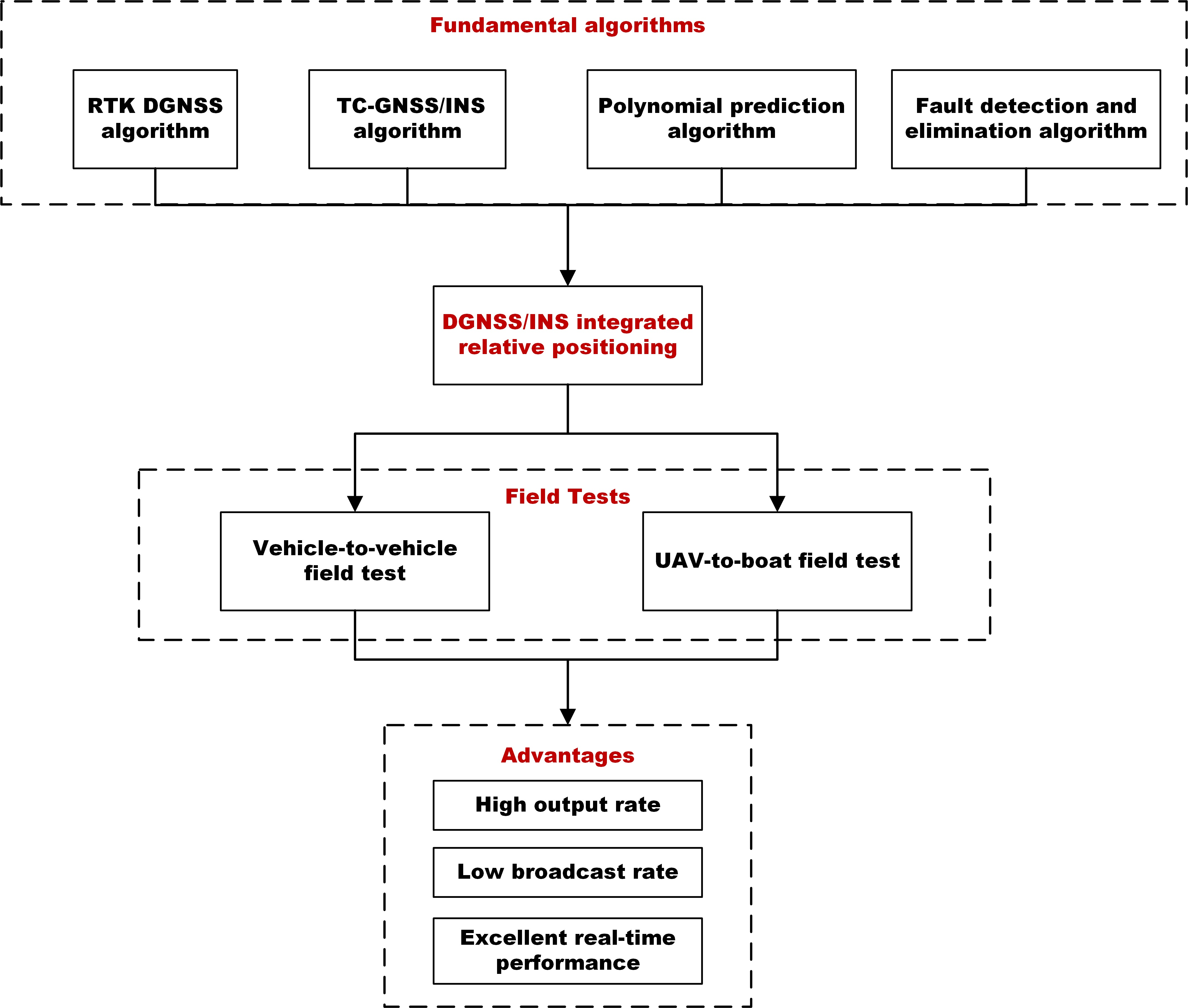
A carrier-phase-based RTK DGNSS relative positioning algorithm is integrated with the carrier-phase-based TC-GNSS/INS integration algorithm to provide high-rate, precise, relative position solutions. Figure 1 displays the overall architecture of the DGNSS/INS integration relative positioning system, which is composed of four parts, i.e., the rover system, a moving base system, GNSS and datalink. $f$ denotes accelerometer measurements, $\omega$ denotes gyroscope measurements, $\rho$ denotes pseudo-range observations and $\varphi$ denotes carrier phase observations. GNSS satellite signals are received synchronously by the GNSS receivers of rover and moving base systems. As for moving base system, carrier phase and pseudo-range observations from GNSS receivers are integrated with the INS measurements from the inertial measurement units (IMUs) in the TC-GNSS/INS integration algorithm to provide the absolute position of the moving base and position increments for the radio station to broadcast. Then, raw GNSS observations and position increments of the moving base are sent to the rover system by wireless datalink. As for the rover system, the RTK DGNSS relative positioning algorithm and TC-GNSS/INS integration algorithm are independent from one another. When no data are being broadcast from the moving base, the TC-GNSS/INS integration algorithm can provide the absolute position of the rover independently. When raw GNSS observations of the moving base are received by the radio station of the rover, the carrier phase and pseudo-range observations of the two receivers are used to construct double-differenced observations between satellites and receivers to calculate the relative distance between the rover and moving base via the RTK DGNSS relative positioning algorithm. When position increments from the moving base are received by the radio station of the rover, the position increments of the rover and moving base and the relative position from RTK DGNSS are merged to obtain the instantaneous synchronous relative position by the integration method. Additionally, single- and dual-station fault detection and elimination (FDE) are carried out before GNSS observations are processed in the positioning algorithms to guarantee the reliability of the solution. The word “single-station” means that the data used for FDE can only be obtained from the GNSS receiver and IMU of a single station, while “dual-station” means that the data from the datalink can also be used. The results of a single-station FDE will be used in the dual-station FDE process inrover.

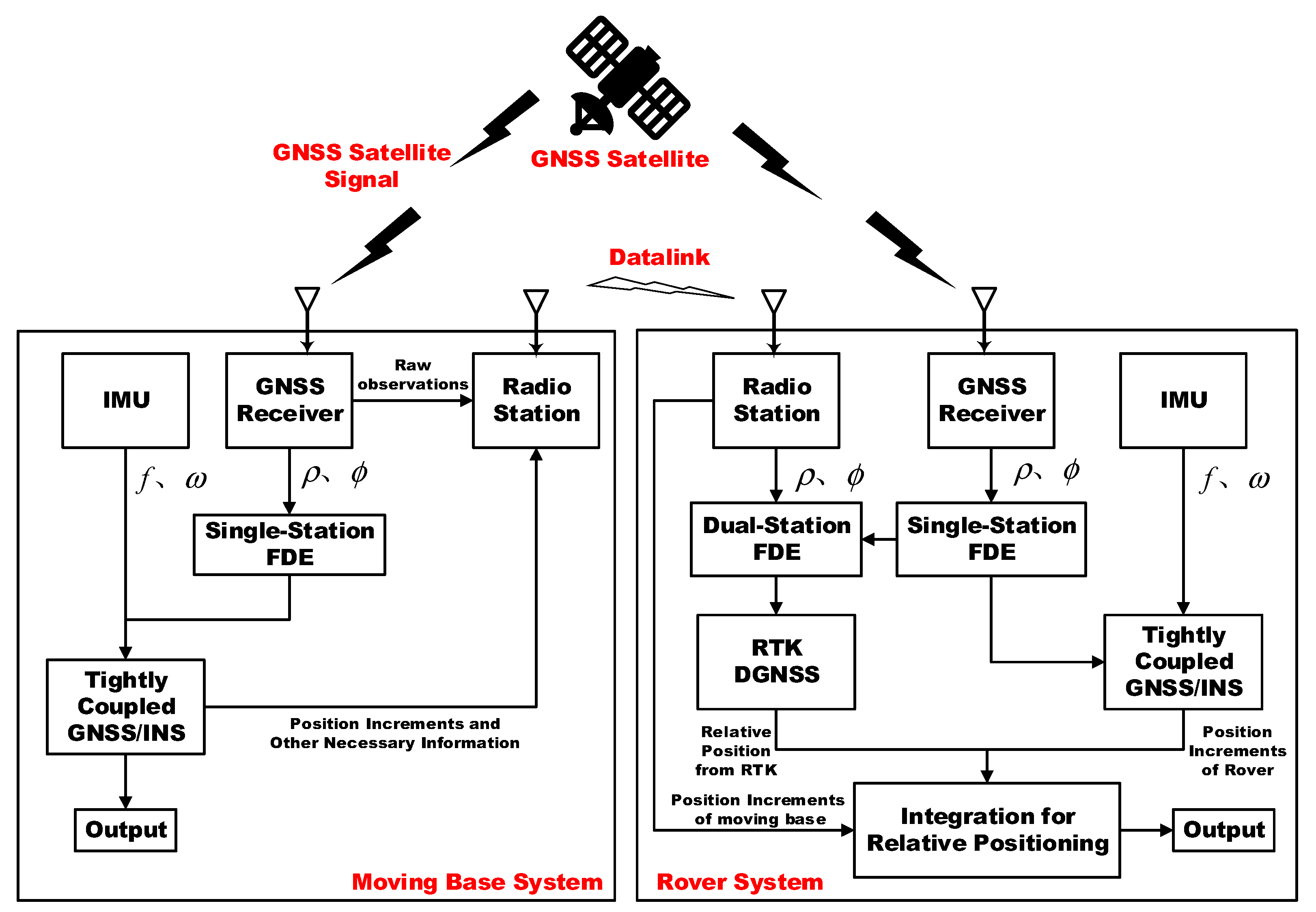
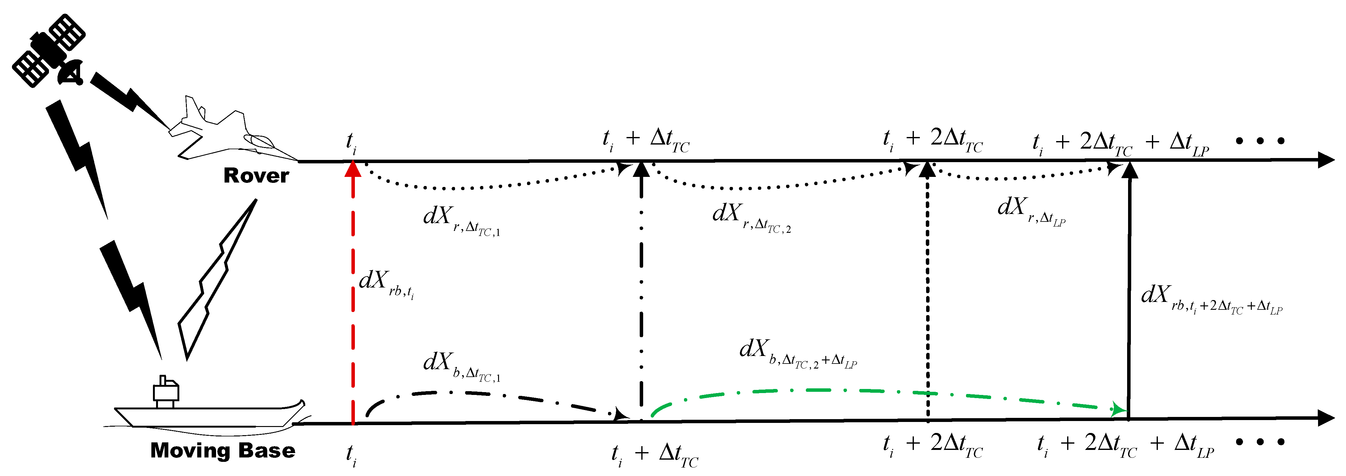
The integration mechanism of the synchronous relative position is displayed in Figure 2. In the figure, the horizontal axis with arrows denotes the observation time axis; $t_0$ and $t_i$ denote the first and i-th observation times, respectively, when the RTK DGNSS relative positioning succeeds; $\mathsf{\Delta }{t}_p$ denotes the time interval for predictions of position increments of the moving base; $\mathsf{\Delta }{t}_{TC}$ denotes the time interval of measurement updates in the TC-GNSS/INS integration algorithm, which is assumed to be the same value in the rover and the moving base. Once RTK DGNSS relative positioning succeeds at $t_0$ and $t_i$, precise baseline vectors $d{\mathit{X}}_{rb,t_0}$ and $d{\mathit{X}}_{rb,t_i}$ between the rover and moving base can be obtained, represented by red dashed vertical arrows in Figure 2. Position increments from $t_i$ to $t_i+\mathsf{\Delta }{t}_{TC}$ can be calculated and saved in a buffer in the rover and moving base independently at $t_i+\mathsf{\Delta }{t}_{TC}$, which are denoted as $d{\mathit{X}}_{r,\mathsf{\Delta }{t}_{TC,1}}$ and $d{\mathit{X}}_{b,\mathsf{\Delta }{t}_{TC,1}}$, represented by black curved dotted arrows in Figure 2. Then, position increments of the moving base, namely $d{\mathit{X}}_{b,\mathsf{\Delta }{t}_{TC,1}}$, are broadcast to the rover. Assuming that the current observation time is $t_i+\mathsf{\Delta }{t}_{TC}+\mathsf{\Delta }{t}_p$, when the nearest RTK DGNSS relative positioning succeeding time is $t_i$ and the time of the latest position increments received from the moving base is $t_i+\mathsf{\Delta }{t}_{TC}$, the integrated synchronous relative position can be expressed as

$$d{\mathit{X}}_{rb,t_i+\mathsf{\Delta }{t}_{TC}+\mathsf{\Delta }{t}_p}=d{\mathit{X}}_{rb,t_i}+d{\mathit{X}}_{r,\mathsf{\Delta }{t}_{TC,1}}+d{\mathit{X}}_{r,\mathsf{\Delta }{t}_p}-d{\mathit{X}}_{b,\mathsf{\Delta }{t}_{TC,1}}-d{\mathit{X}}_{b,\mathsf{\Delta }{t}_p}$$

(13)

where $d{\mathit{X}}_{rb,t_i+\mathsf{\Delta }{t}_{TC}+\mathsf{\Delta }{t}_p}$ denotes the integrated synchronous relative position at $t_i+\mathsf{\Delta }{t}_{TC}+\mathsf{\Delta }{t}_p$, which is represented by solid arrows in Figure 2; $d{\mathit{X}}_{r,\mathsf{\Delta }{t}_p}$ denotes the position increment of the rover from $t_i+\mathsf{\Delta }{t}_{TC}$ to $t_i+\mathsf{\Delta }{t}_{TC}+\mathsf{\Delta }{t}_p$, which can be obtained from the TC-GNSS/INS integration algorithm of the rover; $d{\mathit{X}}_{b,\mathsf{\Delta }{t}_p}$ denotes the predicted position increment of the moving base from $t_i+\mathsf{\Delta }{t}_{TC}$ to $t_i+\mathsf{\Delta }{t}_{TC}+\mathsf{\Delta }{t}_p$ by the polynomial prediction algorithm based on historic broadcasted position increments in a sliding window.

The RTK DGNSS relative positioning solutions and position increments of the rover and moving base are saved in a buffer to allow the integration of synchronous relative position. Assuming that RTK DGNSS relative positioning succeeds, the integration of synchronous relative position, as in Equation (13), can occur. As the position increments of the moving base can be predicted by the polynomial prediction algorithm during data outages from the rover system, the synchronous relative position can be integrated using Equation (13) at an ultra-high rate, i.e., the same as the output rate of the TC-GNSS/INS integration algorithm of the rover.

Broadcast latency of communication packets is a common problem in real-time relative positioning. The proposed navigation architecture solves this problem. Figure 3 shows the synchronous relative position integration mechanism under a condition of broadcast latency of the position increment. $\mathsf{\Delta }{t}_{LP}$ denotes the broadcast latency, while the current observation time is $t_i+2\mathsf{\Delta }{t}_{TC}+\mathsf{\Delta }{t}_{LP}$. This means that there is a latency of position increments at $t_i+2\mathsf{\Delta }{t}_{TC}$. The relative position of the current observation time can still be integrated as

$$d{\mathit{X}}_{rb,t_i+2\mathsf{\Delta }{t}_{TC}+\mathsf{\Delta }{t}_{LP}}=d{\mathit{X}}_{rb,t_i}+{\displaystyle \sum _{j=1}^{2}d{\mathit{X}}_{r,\mathsf{\Delta }{t}_{TC,j}}}+d{\mathit{X}}_{r,\mathsf{\Delta }{t}_{LP}}-d{\mathit{X}}_{b,\mathsf{\Delta }{t}_{TC,1}}-d{\mathit{X}}_{b,\mathsf{\Delta }{t}_{TC,2}+\mathsf{\Delta }{t}_{LP}}$$

(14)

where $d{\mathit{X}}_{r,\mathsf{\Delta }{t}_{LP}}$ denotes the position increment of the rover from $t_i+2\mathsf{\Delta }{t}_{TC}$ to $t_i+2\mathsf{\Delta }{t}_{TC}+\mathsf{\Delta }{t}_{LP}$, as calculated by the TC-GNSS/INS integration algorithm, and $d{\mathit{X}}_{b,\mathsf{\Delta }{t}_{TC,2}+\mathsf{\Delta }{t}_{LP}}$ denotes the predicted position increment of the moving base from $t_i+\mathsf{\Delta }{t}_{TC}$ to $t_i+2\mathsf{\Delta }{t}_{TC}+\mathsf{\Delta }{t}_p$, calculated by the polynomial prediction algorithm, which is represented by green dotted arrows in Figure 3. Position increments from the moving base should be received at $t_i+2\mathsf{\Delta }{t}_{TC}$. The blank of the relative positions caused by the latency of position increments can be filled in by the integration mechanism. It is worth noting that the broadcast latency of position increments makes the maximal prediction time of position increments of the moving base longer, thereby reducing the prediction accuracy.

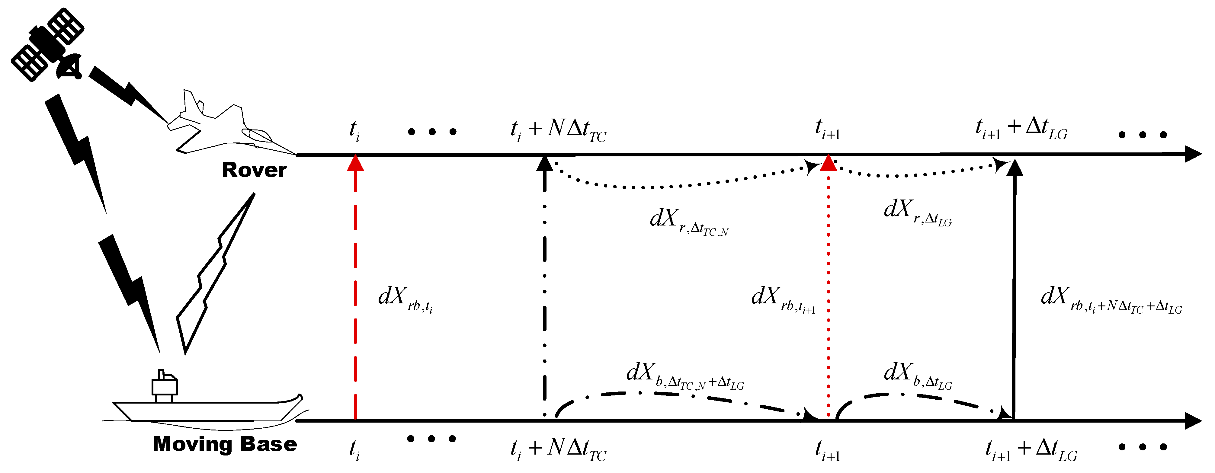
Figure 4 shows the integration mechanism of synchronous relative position in the presence of broadcast latency affecting the raw GNSS observations. $N$ denotes the total number of position increments between adjacent RTK DGNSS relative positions; $\mathsf{\Delta }{t}_{LG}$ denotes the broadcast latency; $t_{i+1}$ denotes the time when the RTK DGNSS relative position can be obtained; and $d{\mathit{X}}_{rb,t_{i+1}}$ denotes the corresponding relative position, which is represented by red dotted vertical arrows. The current observation time is $t_i+N{t}_{TC}+\mathsf{\Delta }{t}_{LG}$, where $t_{i+1}=t_i+N{t}_{TC}$. If the raw GNSS observations of the moving base at $t_{i+1}$ are received in a timely manner by the rover, $d{\mathit{X}}_{rb,t_{i+1}}$ can be obtained and used in the integration process. However, $d{\mathit{X}}_{rb,t_{i+1}}$ cannot be obtained due to the latency of the raw GNSS observations from the moving base. The most recent historical baseline vectors between the rover and moving base can be used in the integration process in such a case. Therefore, the relative position of the current observation time can still be integrated as

$$d{\mathit{X}}_{rb,t_i+N{t}_{TC}+\mathsf{\Delta }{t}_{LG}}=d{\mathit{X}}_{rb,t_i}+{\displaystyle \sum _{j=1}^{N}d{\mathit{X}}_{r,\mathsf{\Delta }{t}_{TC,j}}}+d{\mathit{X}}_{r,\mathsf{\Delta }{t}_{LG}}-{\displaystyle \sum _{j=1}^{N}d{\mathit{X}}_{b,\mathsf{\Delta }{t}_{TC,j}}}-d{\mathit{X}}_{b,\mathsf{\Delta }{t}_{LG}}$$

(15)

where $d{\mathit{X}}_{r,\mathsf{\Delta }{t}_{LG}}$ denotes the position increment of the rover from $t_{i+1}$ to $t_{i+1}+\mathsf{\Delta }{t}_{LG}$, calculated by the TC-GNSS/INS integration algorithm; $d{\mathit{X}}_{b,\mathsf{\Delta }{t}_{LG}}$ denotes the position increment of the moving base from $t_{i+1}$ to $t_{i+1}+\mathsf{\Delta }{t}_{LG}$, as predicted by the polynomial prediction algorithm. Blank relative positions caused by the latency of raw GNSS observations can be filled in by constructing the most recent RTK DGNSS relative position and summing the position increments. It is also worth noting that broadcast latency of raw GNSS observations will increase the cumulative error of the position increments.

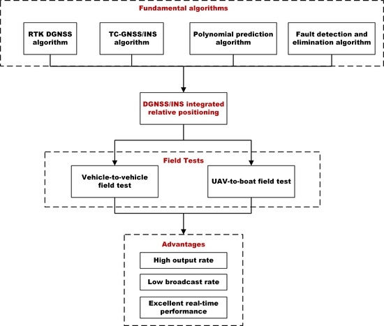
The proposed method can not only provide precise relative positions at an ultra-high rate, but can also overcome the adverse effect of broadcast latency of position increments and raw GNSS observations on the real-time performance. Four kinds of fundamental algorithms, namely, the RTK DGNSS relative positioning algorithm, TC-GNSS/INS integration algorithm, prediction algorithm for position increments and the FDE algorithm are combined in the method. The RTK DGNSS relative positioning algorithm and TC-GNSS/INS integration algorithm are basic algorithms. The prediction algorithm for position increments and FDE algorithm are used to improve the output rate, accuracy and reliability of the relative positioning solutions introduced in the subsequent sections.

Last but not least, we note that the proposed method also shows benefits in terms of reducing the broadcast and sampling rates. If only RTK DGNSS relative solutions are applied, the output rate will be determined by the broadcast and sampling rates of the raw GNSS observations. Thus, communication burden will be heavy for high-rate output. With the help of position increments, as determined by the TC-GNSS/INS integration algorithm of the rover and moving base, the broadcast and sampling rates of raw GNSS observations can be greatly reduced. With the help of position increments predicted by the polynomial prediction algorithm, the broadcast rate of position increments can also be reduced. However, prediction time cannot be too long, i.e., the broadcast rate of position increments should remain relatively high, especially for complex motion conditions. Fortunately, position increment datasets are small, unlike raw GNSS observations. Thus, the broadcast rate of position increments can be increased appropriately. On the other hand, as short-term, precise position increments can be provided by the TC-GNSS/INS integration algorithm, the sampling rates of receivers can be reduced to reduce computational load and power consumption. Additionally, if the motion state of the moving base is simple, e.g., a straight line, the broadcast rate of the position increments of the moving base can also be reduced. A detailed analysis of the effects of the data broadcast rate and sampling rate will be carried out based on two field tests in Section 3.1.

2.4. Polynomial Prediction Algorithm for Position Increments

In order to obtain synchronous relative position during position increment broadcast outages from the moving base, the polynomial prediction algorithm based on historical broadcasted position increments in a sliding window is adopted. The polynomial model is defined as

$${\nu }_{{\tau }_i}={\alpha }_0+{\alpha }_1{\tau }_i+{\alpha }_2{\tau }_i^2+\dots +{\alpha }_p{\tau }_i^p$$

(16)

where $\nu$ denotes the variable to be modeled; ${\tau }_i$ denotes the relative time, where origin is the time of the first element of the sliding window; $p$ denotes order; and $\alpha$ denotes polynomial coefficients. $\nu$ and ${\tau }_i$ can be calculated by

$$\{\begin{array}{l}{\tau }_i=t_{i,real}-t_{1,real}\\ {\nu }_{{\tau }_i}=d{\mathit{X}}_{b,\mathsf{\Delta }{t}_{TC}}(t_{i,real})/\mathsf{\Delta }{t}_{TC}\end{array}$$

(17)

where $t_{1,real}$ denotes the real end observation time of the first position increment in the sliding window; $t_{i,real}$ denotes the real end observation time of the i-th position increment in the sliding window; and $\mathsf{\Delta }{t}_{TC}$ denotes the coasting time of position increments. When the number of elements in the sliding window is greater than $p+1$, all the polynomial coefficients can be determined by LSE. Then, the predicted position increment of the moving base at $t_{c,real}$ can be calculated as

$$\{\begin{array}{l}{\tau }_c=t_{c,real}-t_{1,real}\\ {\nu }_{{\tau }_c}={\alpha }_0+{\alpha }_1{\tau }_c+{\alpha }_2{\tau }_c^2+\dots ++{\alpha }_p{\tau }_c^p\\ d{\mathit{X}}_{b,\mathsf{\Delta }{t}_{TC}}(t_{c,real})={\nu }_{{\tau }_c}\mathsf{\Delta }{t}_{TC}\end{array}$$

(18)

2.5. FDE Algorithm

Outliers in GNSS observations should be detected and eliminated before observations are used for relative positioning. Carrier phase cycle slip and pseudo-range outliers are the most common faults. Multiple methods have been designed and combined to detect and eliminate these faults.

As for carrier phase cycle slips, the classic geometry-free carrier phase combination (GF) method is combined with the INS-aided cycle slip detection method to detect and simultaneously exclude single- or double-frequency cycle slips in different satellites. The test statistic of the GF method and the corresponding variance are constructed as

$$\{\begin{array}{l}{T}_{gf,i}={\lambda }_{f_1}{\mathsf{\Delta }}_t{\varphi }_{v,f_1}^i-{\lambda }_{f_2}{\mathsf{\Delta }}_t{\varphi }_{v,f_2}^i\\ {\sigma }_{gf,i}^2={\lambda }_{f_1}^2{\sigma }_{{\mathsf{\Delta }}_t{\varphi }_{v,f_1}^i}^2+{\lambda }_{f_1}^2{\sigma }_{{\mathsf{\Delta }}_t{\varphi }_{v,f_1}^i}^2\end{array}$$

(19)

where $i$ denotes the number of the satellite to be detected; $v$ denotes the number of the station; $f_1$ and $f_2$ denote two different signal frequencies; $\lambda$ denotes wavelengths; ${\sigma }^2$ denotes variance; $\varphi$ is the carrier phase observation, which can be in undifferenced (UD), single-differenced (SD) or double-differenced (DD) form; finally, ${\sigma }_{{\mathsf{\Delta }}_t{\varphi }_{v,f_1}^i}^2$ and ${\sigma }_{{\mathsf{\Delta }}_t{\varphi }_{v,f_2}^i}^2$ are a priori information, which is given according to the statistical characteristics of the carrier phase. To simplify the present description, we define the GF method with the UD, SD between satellites, SD between receivers and DD between satellites and receivers as the UD GF method, BS-SD GF method, BR-SD GF method and DD GF method, respectively. The GF method shows excellent performance in terms of detecting small cycle slips, but it cannot detect special dual-frequency cycle slips. Additionally, it cannot identify single-frequency cycle slips and requires the use of a dual-frequency receiver.

The INS-aided cycle slip detection method can overcome defects in the GF method. Its test statistics for single-station combination observations and corresponding variance are constructed as

$$\{\begin{array}{l}{T}_{\mathit{s},i,f,v,\varphi }={\lambda }_f{\mathsf{\Delta }}_t{\varphi }_{v,f}^{in}+c{\mathsf{\Delta }}_t\delta t^{in}-{\mathsf{\Delta }}_t{R}_{v,in\mathit{s}}^{in}\\ {\sigma }_{\mathit{s},i,f,v,\varphi }^2={\lambda }_f^2{\sigma }_{{\mathsf{\Delta }}_t{\varphi }_{v,f}^{in}}^2+ {\sigma }_{{\mathsf{\Delta }}_t{R}_{v,in\mathit{s}}^{in}}^2\end{array}$$

(20)

where $n$ denotes the number of the reference satellites, $f$ denotes the signal frequency, $c$ denotes the speed of light, $\delta t$ denotes satellite clock error, and $R_{v,in\mathit{s}}$ denotes the satellite-receiver range, which can be expressed as

$$R_{v,in\mathit{s}}^{in}=(\left|{\mathit{r}}^i-{\widehat{\mathit{r}}}_v\right|)-(\left|{\mathit{r}}^n-{\widehat{\mathit{r}}}_v\right|)$$

(21)

where ${\mathit{r}}^i$ denotes the position of satellite $i$; ${\widehat{\mathit{r}}}_v$ denotes the position of station $v$, as predicted by INS, which is calculated by the TC-GNSS/INS integration algorithm; and ${\sigma }_{{\mathsf{\Delta }}_t{\varphi }_{v,f}^{in}}^2$ is a priori information. ${\sigma }_{{\mathsf{\Delta }}_t{R}_{v,in\mathit{s}}^{in}}^2$ is also calculated by the TC-GNSS/INS integration algorithm. In the present description, this kind of INS-aided method is referred to as the BS-SD INS-aided method.

When the observations and absolute position of the moving base are received by the rover, a test statistic for dual-station combination observations and the corresponding variance can be constructed as

$$\{\begin{array}{l}{T}_{d,i,f,vw,\varphi }={\lambda }_f{\mathsf{\Delta }}_t{\varphi }_{vw,f}^{in}-{\mathsf{\Delta }}_t{R}_{vw,in\mathit{s}}^{in}\\ {\sigma }_{d,i,f,vw,\varphi }^2={\lambda }_f^2{\sigma }_{{\mathsf{\Delta }}_t{\varphi }_{vw,f}^{in}}^2+ {\sigma }_{{\mathsf{\Delta }}_t{R}_{vw,in\mathit{s}}^{in}}^2\end{array}$$

(22)

where $R_{vw,in\mathit{s}}$ can be expressed as

$$R_{vw,in\mathit{s}}^{in}=(\left|{\mathit{r}}^i-{\widehat{\mathit{r}}}_v\right|)-(\left|{\mathit{r}}^n-{\widehat{\mathit{r}}}_v\right|)-(\left|{\mathit{r}}^i-{\widehat{\mathit{r}}}_w\right|)-(\left|{\mathit{r}}^n-{\widehat{\mathit{r}}}_w\right|)$$

(23)

where ${\widehat{\mathit{r}}}_w$ denotes position of station $w$ provided by the datalink, which is calculated by the TC-GNSS/INS integration algorithm in the moving base; and ${\sigma }_{{\mathsf{\Delta }}_t{\varphi }_{vw,f}^{in}}^2$ is a priori information. ${\sigma }_{{\mathsf{\Delta }}_t{R}_{v,in\mathit{s}}^{in}}^2$ is also calculated by the TC-GNSS/INS integration algorithm. In the present description, this kind of INS-aided method is referred to as the DD INS-aided method. By combining the GF and INS-aided methods, all kinds of cycle slips can be detected and excluded.

As for pseudo-range outliers, considering the poor detection performance of GNSS methods alone, we only use INS-aided outlier detection methods for single- and dual-station combination observations. The construction of test statistics and the corresponding variance of a single-station is expressed as

$$\{\begin{array}{l}{T}_{\mathit{s},i,f,v,P}=P_{v,f}^{in}+c\delta t^{in}-R_{v,in\mathit{s}}^{in}-\delta I_{v,f}^{in}-\delta T_{v,f}^{in}\\ {\sigma }_{\mathit{s},i,f,v,P}^2={\sigma }_{P_{v,f}^{in}}^2+ {\sigma }_{R_{v,in\mathit{s}}^{in}}^2\end{array}$$

(24)

where ${\sigma }_{P_{v,f}^{in}}^2$ is a priori information, which is given according to the statistical characteristics of the pseudo-range; $\delta I$ denotes ionospheric delay, calculated using the dual-frequency ionosphere-free combination [26]; and $\delta T$ is tropospheric delay, corrected by the Saastamoinen model [32]. When there are GNSS observations from two receivers under a short baseline condition, it is assumed that the ionospheric and tropospheric delay are eliminated by the double-differenced combinations between satellites and receivers. The statistic and corresponding variance of the dual-station are constructed as

$$\{\begin{array}{l}{T}_{d,i,f,v,P}=P_{vw,f}^{in}-R_{vw,in\mathit{s}}^{in}\\ {\sigma }_{d,i,f,v,P}^2={\sigma }_{P_{vw,f}^{in}}^2+ {\sigma }_{R_{vw,in\mathit{s}}^{in}}^2\end{array}$$

(25)

All the test statistics mentioned above are assumed to be normal distributions with zero mean and known variance in null hypothesis, in which the mean equals the value of the outlier and the variance is constant in alternative hypotheses. Thus, given the required false alarm risk $P_{FA}$, the test threshold is expressed as

$$T_h=-{\mathsf{\Phi }}^{-1}(\frac{P_{FA}}{2}){\sigma }_T$$

(26)

where ${\sigma }_T$ denotes the standard deviation of the test statistic, which is the root of variance of the test statistic. This can be calculated by (19), (20), (22) and (25), whereby ${\mathsf{\Phi }}^{-1}(\mathit{x})$ is the inverse function of $\mathsf{\Phi }(\mathit{x})$, which is defined as

$$\mathsf{\Phi }(\mathit{x})={\displaystyle {\int }_{-\infty }^{\mathit{x}}\frac{1}{\sqrt{2\pi }}}{e}^{-\frac{{\tau }^2}{2}}d\tau$$

(27)

Let’s assume that $T_{cb}$ represents the test statistic of all of the methods described above, which can be calculated by (19), (20), (22) and (25). If $\left|T_{cb}\right|\le T_h$, the corresponding observations can be used for subsequent relative positioning. As for the GF method, if $\left|T_{cb}\right|>T_h$, both of the two channels, using different frequencies in the corresponding carrier phase observations, should be eliminated. As for INS-aided cycle slip and pseudo-range outlier detection, if $\left|T_{cb}\right|>T_h$, the corresponding single channel of the carrier phase or pseudo-range should be eliminated.

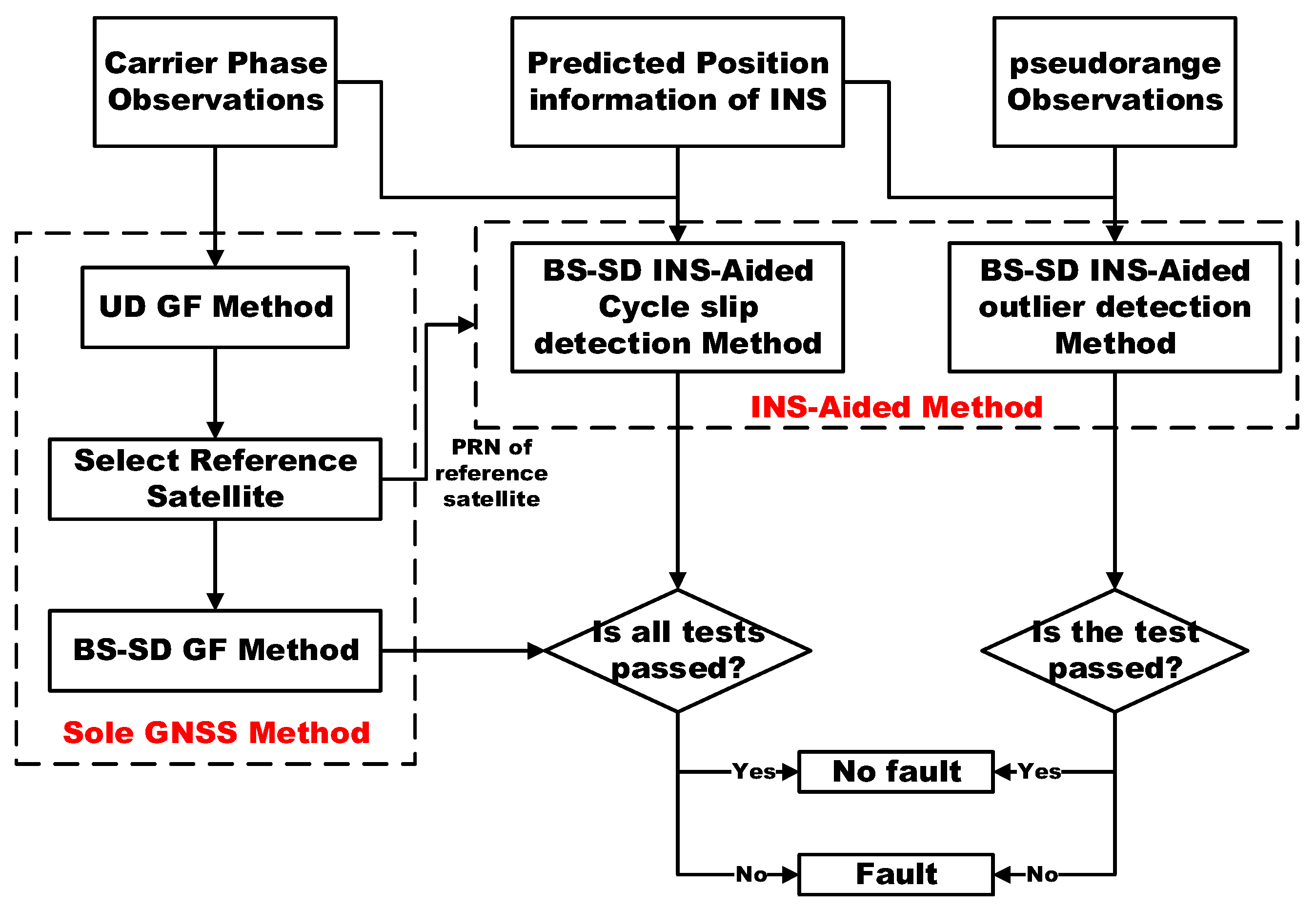
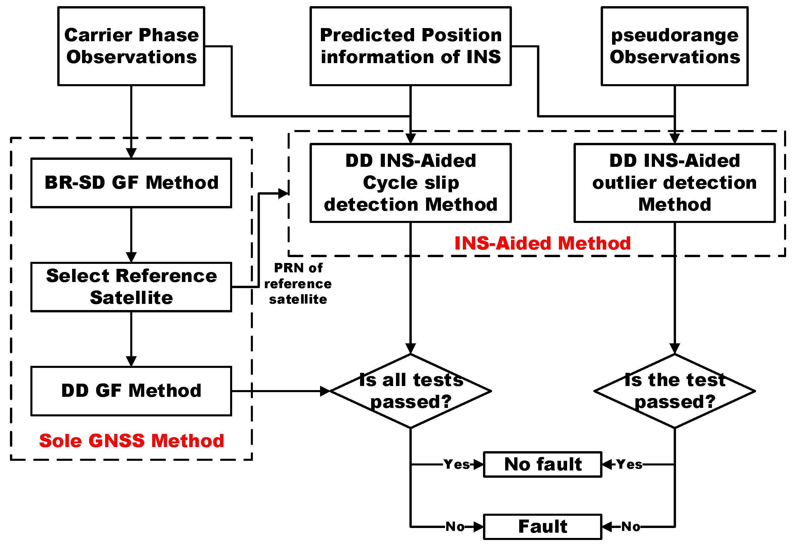
All of these methods are combined to detect and eliminate carrier phase cycle slips and pseudo-range outliers for single- or dual-station combination observations. In order to make the most of the advantages of each method, we designed a combined fault detection rule for single- and dual-station fault detection, as shown in Figure 5 and Figure 6. Use of the GNSS method alone means that only GNSS observations are used to construct test statistics, while the implementation of the INS-aided method facilitates the solutions of the TC-GNSS/INS integrated algorithm. The UD GF and BR-SD GF methods are used to prevent faulty satellites from being taken as the reference satellite before SD operations among satellites and DD operation are carried out. Then, the GNSS and INS-aided methods are combined to detect faults. Once a fault is detected, the corresponding satellite is eliminated in the subsequent positioning calculation.

3. Field Tests and Results Analysis

Two field tests were designed to validate the performance of the proposed method in different application scenarios. A vehicle-to-vehicle field test was carried out in Changsha, Hunan Province, China on 27 November 2017, referred as ‘test 1’. In test 1, both the rover and moving base were vehicles which moved erratically in an open space, as shown in Figure 7. A static reference station with a pre-surveyed position was set nearby for post-processing of the synchronous DGNSS relative positions of the moving base and rover. The corresponding results were used to calculate a reference value for the position increment and relative position solutions. The trajectories and velocities of the two vehicles are shown in Figure 8 and Figure 9. A UAV-to-boat field test was carried out in the nearby Liangzi Lake, Hubei Province, China on 23 November 2019, referred as ‘test 2’, where UAV refers an unmanned aerial vehicle. In test 2, the UAV was the rover and the boat was the moving base, as shown in Figure 10. The UAV flew at an altitude of about 300 m, nearly in a straight line, while the boat sailed in the lake nearly in a straight line, as shown in Figure 11. A static reference station with a pre-surveyed position was set nearby for post-processing of the synchronous DGNSS relative positions of the UAV and boat. The velocities of the UAV and boat are shown in Figure 12.

In the two tests, a GNSS/MEMS prototype system, consisting of a Sensonor STIM300 MEMS and ComNav OEM-K508 board, was mounted on both the rover and moving base. The GNSS receiver can provide five frequency observations of BDS/GPS (B1/B2/B3/L1/L2) for real-time navigation and post-processing. Only four BDS/GPS (B1/B3/L1/L2) frequency observations are used in the following analysis. The maximal sampling rate of the GNSS receiver is 10 Hz, and the sampling rate of the MEMS is 125 Hz. Xtend-PKG 900 MHz RF modems from Digi International Inc. were used to transmit and receive the data packets. Raw GNSS observations are broadcast in the multiple signal message 5 (MSM 5) format of RTCM 3.2 message format for differential positioning data communication. In order to analyze the accuracy of the position increments and the integrated synchronous relative position, reliable post-processed DGNSS relative positioning results for the rover relative to the static reference station, and the moving base relative to the static reference station are used to provide reference values. The number of visible satellites in the field tests is shown in Figure 13 (15° elevation mask).

3.1. Analysis of the Effect of Data Broadcast Rate and Sampling Rate

If RTK DGNSS relative positioning is adopted to provide relative positions with a high output rate, the sampling rate of the GNSS receiver and broadcast rate between receivers should be increased by the same rate, which will increase the pressure of data communication and processing. The proposed method effectively solves this problem. According to the analysis in Section 2.3, the integrated synchronous relative position consists of the synchronous relative position of the RTK DGNSS relative positioning, position increments of TC-GNSS/INS integration algorithm in the rover and moving base and the position predictions of the moving base. As discussed in the introduction, centimeter-level accuracy of relative positions and position increments can be achieved by RTK DGNSS relative positioning and the TC-GNSS/INS integration algorithm, respectively. However, the effects of the sampling and data broadcast rates on position predictions for a moving base have not been widely studied to date.

The polynomial prediction algorithm is implemented by the rover during position increment broadcast outages from the moving base, indicating that the prediction accuracy depends on the accuracy of historic position increments broadcast by the moving base and the broadcast rate of position increments of thereof (BRPM). Assuming that the broadcast rate of GNSS observations of the moving base (BRGM) is the same as the sampling rate of the GNSS observations thereof (SRGM), and the position increments of the moving base are usually broadcast simultaneously with GNSS observations, the maximum prediction time of position increments depends on BRPM. After carrying out a comprehensive analysis with massive data offline and considering the real-time applications, the order of the polynomial algorithm was set as 2 and the size of the sliding window at 10 epochs, which means that ten historical position increments are used in the prediction algorithm each time.

Table 1. RMSE of predictions of position increments.

BRPM	10		5		2		1
Field Test	Test 1	Test 2	Test 1	Test 2	Test 1	Test 2	Test 1	Test 2
North (m)	0.0050	0.0018	0.0194	0.0022	0.2933	0.0037	1.2487	0.0068
East (m)	0.0051	0.0017	0.0193	0.0022	0.2864	0.0035	0.8713	0.0065
Down (m)	0.0058	0.0043	0.0068	0.0043	0.0094	0.0050	0.0154	0.0065
3D (m)	0.0092	0.0049	0.0282	0.0053	0.4100	0.0071	1.5227	0.0115

shows the statistical results of position prediction errors at different BRPM in the two tests. Figure 14 displays a comparison of the RMSE of the prediction of position increments in the two tests. In test 1, it is clear that the prediction error degrades quickly in the horizontal direction with increasing prediction time, while the prediction error degrades slowly in vertical direction. The reason for this is that the moving base typically moves horizontally, while vertical direction changes are minimal. In test 2, the prediction error degrades slowly with increasing prediction time; however, the accuracy of the prediction error remains at the centimeter level, even when the prediction time is 1 s. The reason for this is that the motion mode of moving base in test 2 is simple. As the movements were more erratic in test 1, a higher position increment broadcast rate of the moving base can provide more accurate information for predictions. Thus, the position increment broadcast rate should remain relatively high when the moving base is changing position erratically.

Here, the effects of the broadcast rate of position increments and the sampling rate of the GNSS receiver on the prediction errors in test 1 are analyzed in more detail. Assuming that the frequency of measurement updates of the TC-GNSS/INS integration algorithm in the moving base is the same as that of SRGM, the maximum coasting time of the position increments of the moving base depends on SRGM. Figure 15 displays a comparison of the accuracy of the prediction error with different SRGM–BRPM combinations. For example, 1–10 means that the sampling rate of the GNSS receiver is 1 Hz and the 1-s position increment during sampling period is divided into 10 parts with equal 0.1-s prediction times for broadcasts. As for Figure 15a, SRGM is fixed as 1 Hz and four different broadcast rates are compared. It is obvious that increasing the broadcast rate significantly improves the prediction accuracy. A high broadcast rate can provide time-intensive data for the sliding window. When the moving base moves erratically, a smaller time interval can reflect more motion characteristics, and therefore, a high broadcast rate can improve the prediction accuracy significantly. As for Figure 15b, BRPM is fixed at 10 Hz and four different sampling rates are compared. It can be seen that increasing the sampling rate only has a slight impact on the prediction accuracy. This means that centimeter-level-accuracy prediction increments can still be provided by the polynomial algorithm at a low receiver sampling rate and appropriately high broadcast rate of position increments from the moving base when the motion thereof is complex. Compared with the raw GNSS observations, the data of position increments are small. Thus, increasing the position increment broadcast rate may be appropriate.

3.2. Performance of Relative Positioning in a Vehicle-to-Vehicle Field Test

Based on the analysis in the former section, six sampling and broadcast rate modes are designed for test 1, where mode 0 is for the RTK DGNSS relative positioning method and modes 1–5 are for the proposed method, as shown in

Table 2. Modes of sampling and broadcast rate in test 1.

Items	Mode 0	Mode 1	Mode 2	Mode 3	Mode 4	Mode 5
BRGM (Hz)	10	10	1	1	1	1
BRPM (Hz)	0	10	10	10	5	1
SRGM (Hz)	10	10	10	1	1	1
SRGR (Hz)	10	10	10	1	1	1
Output Rate (Hz)	10	125	125	125	125	125
Bit Rate (bits/s)	37,200	42,320	8840	8840	6280	4232

. SRGR indicates the sampling rate of the GNSS observations of the rover. As the same type of GNSS receiver is used by both the rover and the moving base, SRGM and SRGR are always the same in the table. The relative position output rate is 125 Hz in modes 1–5 but 10 Hz in mode 0. According to the communication format of RTCM 3.2, assuming that there are dual-frequency observations from 10 visible satellites of GPS and BDS respectively, the communication cost will be 3720 bits for every communication packet of raw GNSS observations. The communication format of position increments and related necessary data was defined by us: 512 bits in each communication packet. The data broadcast rates, i.e., the bit rate, of the different modes in Table 2 are calculated based on these two typical values.

Table 3. Relative position errors in test 1.

Statistics		Mode 1	Mode 2	Mode 3	Mode 4	Mode 5
Maximum Error (m)	North	0.0205	0.0198	0.0973	0.0974	2.6945
	East	0.0231	0.0244	0.0887	0.0885	2.2124
	Down	0.0384	0.0387	0.1260	0.1259	0.1257
RMSE (m)	North	0.0044	0.0044	0.0111	0.0158	0.6364
	East	0.0047	0.0047	0.0109	0.0159	0.4635
	Down	0.0086	0.0087	0.0202	0.0203	0.0216
	3D	0.0107	0.0108	0.0255	0.0302	0.7875

displays the statistical results of the relative position errors of the proposed method in test 1. Figure 16 shows a comparison of the relative position errors of modes 1–4 in test 1.

Compared with mode 1, mode 2 only significantly decreases the broadcast rate of raw GNSS observations from 10 Hz to 1 Hz, while leaving other parameters unchanged. According to Table 3, the accuracy of relative position errors in both modes is very close, with the same high-rate output in this case as that displayed in Figure 16. Figure 17 shows error scatterplots of modes 1 and 2. It can be seen that errors are distributed in a very small range and are very close between the two modes. It is worth noting that the data broadcast rate in mode 2 is reduced by 79.11% compared to mode 1. This proves that the broadcast rate of raw GNSS observations can be greatly reduced, which has a slight effect on the relative position accuracy.

Compared with mode 2, mode 3 only significantly decreases the sampling rate of the GNSS receivers of the rover and moving base from 10 Hz to 1 Hz; all other parameters remain unchanged. The data broadcast rates of these two modes are the same. The maximal coasting time of the position increments increases from 0.1 s to 1 s due to the decrease of the sampling rate, which is the reason for the decline in the accuracy of relative position error of mode 3, as shown in Figure 16. Figure 18 shows error scatterplots of modes 2 and 3. The distribution range of errors in mode 3 is obviously larger than that of mode 2, which reflects the effect of decreasing the sampling rate of the GNSS receivers, as discussed in the previous section. Though a decreased sampling rate degrades the accuracy of the relative position, the accuracy is still high enough for kinematic applications. Thus, it may be worth sacrificing a little accuracy to significantly reduce the computational load and power consumption by decreasing the sampling rate.

Compared with mode 3, modes 4 and 5 only significantly decrease the broadcast rate of position increments of the moving base from 10 Hz to 5 Hz and 1 Hz; all other parameters remain unchanged. The relative position error in the horizontal direction degrades dramatically with a decrease of the broadcast rate, as shown in

Table 4. RMSE with different minimal latencies of position increments in mode 3.

Minimal Latency (s)	0	0.1	0.2	0.3	0.4
North	0.0111	0.0150	0.0283	0.0515	0.0829
East	0.0109	0.0150	0.0282	0.0520	0.0849
Down	0.0202	0.0210	0.0229	0.0265	0.0333
3D	0.0255	0.0299	0.0461	0.0778	0.1233

. The accuracy of mode 5 even degrades to the decimeter level. Figure 19 displays error scatterplots for modes 3 and 4. Obvious degradation can also be seen in the horizontal direction, although the accuracy of mode 4 remains at the centimeter level. The vertical error suffers from no obvious degradation with a decrease in the broadcast rate. This phenomenon is consistent with the analysis in the previous section; the reason for it is that the moving base moves horizontally. Additionally, we find that the vertical error is also very close between modes 1 and 2 or modes 3 and 4. This means that the sampling rate of the GNSS receivers of the rover and moving base are the most influential factors on vertical error.

Compared with 10-Hz output of sole RTK DGNSS relative positioning, modes 2, 3 and 4 can provide 125-Hz, centimeter-level-accuracy relative positions with data broadcast rates reduced by 76.24%, 76.24% and 83.12%, respectively. Additionally, the sampling rate can also be reduced from 10 Hz to 1 Hz in modes 3 and 4.

In order to validate the real-time performance of the proposed method, the latencies of position increments and raw GNSS observations are simulated for post processing with the logged raw data. The minimum latency in the post-simulation experiment is set independently for position increments and raw GNSS observations. Table 4 and

Table 5. RMSE with different minimal latencies of raw GNSS observations in mode 3.

Minimal Latency (s)	0	0.1	0.2	0.3	0.4
North	0.0111	0.0150	0.0283	0.0515	0.0829
East	0.0109	0.0150	0.0282	0.0520	0.0849
Down	0.0202	0.0210	0.0229	0.0265	0.0333
3D	0.0255	0.0299	0.0461	0.0778	0.1233

show the statistical RMS under conditions of different minimal latency of position increments and raw GNSS observations in mode 3. Obviously, the relative position accuracy will deteriorate with an increase of simulated minimal latency. As for position increments, the accuracy of three components can remain at the centimeter level when the minimal latency is less than or equal to 0.4 s, which means that four consecutive packet drops of position increments can be tolerated in mode 3 in the proposed method. As for raw GNSS observations, the accuracy of horizontal direction decreases slowly, unlike that of vertical direction. The accuracy of three components can remain at the centimeter level when the minimal latency is less than or equal to 2.5 s, which means that two consecutive packet drops of raw GNSS observations can be tolerated in mode 3. Generally, the value of communication latency is at a millisecond level, i.e., sometimes up to 100 ms [1]. Thus, the proposed method effectively overcomes the adverse impact of latency and can tolerate a certain number of packet drops.

3.3. Performance of Relative Positioning in a UAV-to-Boat Field Test

As the moving base moves more or less in a straight line in test 2, the position prediction error remains at a centimeter level when the prediction time is 1 s, as discussed in the former section. This means that the broadcast rate of the position increments and raw GNSS observations of the moving base may be further reduced. Four modes of sampling and broadcast rates are designed for test 2 to reduce the data broadcast rate, as shown in

Table 6. Modes of sampling and broadcast rate in test 2.

Items	Mode 0	Mode 5	Mode 6	Mode 7	Mode 8
BRGM (Hz)	10	1	0.5	0.2	0.1
BRPM (Hz)	0	1	1	1	1
SRGM (Hz)	10	1	1	1	1
SRGR (Hz)	10	1	1	1	1
Output Rate (Hz)	10	125	125	125	125
Bit Rate (bits/s)	37,200	4232	2372	1256	884

. The statistical results regarding relative position errors are displayed in

Table 7. Statistical results of relative position errors in test 2.

Statistics		Mode 5	Mode 6	Mode 7	Mode 8
Maximum Error (m)	North	0.0228	0.0282	0.0763	0.1344
	East	0.0272	0.0272	0.0528	0.0740
	Down	0.0628	0.0628	0.0807	0.1288
RMSE (m)	North	0.0050	0.0069	0.0162	0.0288
	East	0.0065	0.0073	0.0116	0.0164
	Down	0.0103	0.0126	0.0191	0.0336
	3D	0.0131	0.0161	0.0276	0.0472

. We find that high-rate, centimeter-level-accuracy relative positions can still be provided in mode 5. As the time interval between adjacent RTK DGNSS relative positions becomes larger, the total number of the used position increments of the rover and moving base becomes bigger, thereby increasing the cumulative error of position increments. Thus, the RMSE increases with a decrease of the broadcast rate of raw GNSS observations, as shown in Figure 20. Error scatters are shown in Figure 21. We find that centimeter-level-accuracy can still be achieved, even when the broadcast rate of raw GNSS observations is 0.1 Hz. Compared with 10-Hz output of RTK GNSS relative positioning, the data broadcast rates of mode 5, mode 6, mode 7 and mode 8 are reduced by 88.62%, 93.62%, 96.62% and 97.62%.

In fact, it may not be necessary to relax the broadcast rate of raw GNSS observations to the level used in mode 8 for practical applications. From another point of view, the RTK DGNSS relative position solutions may be unavailable due to broadcast latency, data packet drops, elimination by the FDE algorithm or other reasons. The results in Table 7 show the potential of the proposed method to tolerate the unavailability of RTK DGNSS relative position solutions. When mode 5 is adopted in practical applications, nine consecutive packet drops of raw GNSS observations can be tolerated to maintain centimeter-level accuracy, according to the results of the test using mode 8.

4. Conclusions

Aiming to provide high-rate, precise relative positions for safety-critical kinematic-to-kinematic applications, we proposed a real-time, high-rate DGNSS/INS integrated precise relative positioning method. The RTK DGNSS relative positioning algorithm, carrier-phase-based TC-GNSS/INS integrated algorithm and polynomial prediction algorithm for position increments were integrated to obtain the synchronous relative position at an ultra-high rate (125 Hz), i.e., the same as the output rate of the TC-GNSS/INS integrated algorithm of the rover. Two field tests were carried out to analyze the effects of the data broadcast rate and sampling rate and the performance of relative positioning. Based on an analysis of the results of these field tests, the following conclusions may be drawn:

(1) The broadcast and sampling rates of raw GNSS observations can be greatly reduced, while the broadcast rate of position increments should remain relatively high when the moving base changes trajectory frequently. When the moving base moves in a straight line, the broadcast rate for position increments can be lower.

(2) High-rate (125 Hz) centimeter-level-accuracy relative positions can be provided by the proposed method even when the broadcast and sampling rates of the raw GNSS observations are reduced from 10 Hz to 1 Hz. The proposed method can provide high-rate, precise relative positions with low data broadcast and sampling rates.

(3) The influence of latency of raw GNSS observations and position increments on the accuracy of relative positions can be effectively overcome by the proposed method. A small number of consecutive packet drops can also be tolerated.

The proposed method is of practical engineering value in kinematic-to-kinematic aircraft applications or even for spacecraft rendezvous and docking scenarios. Future work will concentrate on integrity monitoring of relative position solutions including fundamental error modeling, fault detection and elimination in the measurement domain and integrity risk analysis of real-time relative position.

5. Patents

A patent has been formalized in China (patent number: CN112147663B) based on the work reported in this paper.

References

1. Caveney, D. Cooperative Vehicular Safety Applications. IEEE Control Syst. Mag. 2010, 30, 38–53. [Google Scholar]
2. Martin, S.; Travis, W.; Bevly, D. Performance Comparison of Single and Dual Frequency Closely Coupled GPS/INS Relative Positioning Systems. In Proceedings of the Position Location & Navigation Symposium, San Diego, CA, USA, 25–27 April 2010. [Google Scholar]
3. De Ponte Müller, F. Survey on Ranging Sensors and Cooperative Techniques for Relative Positioning of Vehicles. Sensors 2017, 17, 271. [Google Scholar] [CrossRef] [PubMed] [Green Version]
4. Feng, W.; Zhao, Y.; Zhou, L.; Huang, D.; Hassan, A. Fast cycle slip determination for high-rate multi-GNSS RTK using modified geometry-free phase combination. GPS Solut. 2020, 24, 42. [Google Scholar] [CrossRef]
5. Travis, W.; Martin, S.; Bevly, D.M. Automated short distance vehicle following using a dynamic base RTK system. Int. J. Veh. Auton. Syst. 2011, 58, 126–141. [Google Scholar] [CrossRef] [Green Version]
6. Williamson, W.R.; Abdel-Hafez, M.F.; Rhee, I.; Song, E.; Wolfe, J.D.; Chichka, D.F.; Speyer, J.L. An Instrumentation System Applied to Formation Flight. IEEE Trans. Control Syst. Technol. 2007, 15, 75–85. [Google Scholar] [CrossRef]
7. Chen, P.; Shu, L.; Ding, R.; Han, C. Kinematic single-frequency relative positioning for LEO formation flying mission. GPS Solut. 2015, 19, 525–535. [Google Scholar] [CrossRef]
8. Hwang, S.S.; Speyer, J.L. Collision Detection System Based on Differential Carrier-Phase Global Positioning System Broadcasts. Water Ence Technol. 2015, 61, 1691–1698. [Google Scholar] [CrossRef] [Green Version]
9. Heo, M.B.; Pervan, B. Carrier phase navigation architecture for shipboard relative GPS. IEEE Trans. Aerosp. Electron. Syst. 2006, 42, 670–679. [Google Scholar]
10. Rife, J.; Khanafseh, S.; Pullen, S.; Lorenzo, D.D.; Kim, U.S.; Koenig, M.; Chiou, T.Y.; Kempny, B.; Pervan, B. Navigation, Interference Suppression, and Fault Monitoring in the Sea-Based Joint Precision Approach and Landing System. Proc. IEEE 2009, 96, 1958–1975. [Google Scholar] [CrossRef]
11. Teunissen, P.J.G. A canonical theory for short GPS baselines. Part I: The baseline precision. J. Geod. 1997, 71, 320–336. [Google Scholar] [CrossRef]
12. Zhodzishsky, M.; Vorobiev, M.; Khvalkov, A.; Ashjaee, J. Real-Time Kinematic (RTK) Processing for Dual-Frequency GPS/GLONASS. In Proceedings of the 11th International Technical Meeting of the Satellite Division of the Institute of Navigation (ION GPS 1998), Nashville, TN, USA, 15–18 September 1998. [Google Scholar]
13. Edwards, S.J.; Cross, P.A.; Barnes, J.B.; Betaille, D. A Methodology for benchmarking real time kinematic GPS. Surv. Rev. 1999, 35, 163–174. [Google Scholar] [CrossRef]
14. Xu, P.; Shi, C.; Fang, R.; Liu, J.; Niu, X.; Zhang, Q.; Yanagidani, T. High-rate precise point positioning (PPP) to measure seismic wave motions: An experimental comparison of GPS PPP with inertial measurement units. J. Geod. 2013, 87, 361–372. [Google Scholar] [CrossRef]
15. Shu, Y.; Fang, R.; Li, M.; Shi, C.; Li, M.; Liu, J. Very high-rate GPS for measuring dynamic seismic displacements without aliasing: Performance evaluation of the variometric approach. GPS Solut. 2018, 22, 121. [Google Scholar] [CrossRef]
16. Comstock, S.J. Development of a Low-Latency, High Data Rate, Differential GPS Relative Positioning System for UAV Formation Flight Control; Air Force Institute of Technology: Dayton, OH, USA, 2006. [Google Scholar]
17. Newby, S.; Corcoran, W. What’s New From NovAtel. In Proceedings of the 8th International Technical Meeting of the Satellite Division of the Institute of Navigation (ION GPS 1995), Palm Springs, CA, USA, 12–15 September 1995; pp. 133–140. [Google Scholar]
18. Lawrence, D.G. Reference Carrier Phase Prediction for Kinematic GPS. U.S. Patent No. 5,903,236, 11 May 1999. [Google Scholar]
19. Hatch, R.R.; Sharpe, R.T.; Yang, Y. GPS Navigation Using Successive Differences of Carrier-Phase Measurements. U.S. Patent No. 7,212,155, 1 May 2007. [Google Scholar]
20. Zhang, L.; Lv, H.; Wang, D.; Hou, Y.; Wu, J. Asynchronous RTK precise DGNSS positioning method for deriving a low-latency high-rate output. J. Geod. 2015, 89, 641–653. [Google Scholar] [CrossRef]
21. Dong, Y.; Zhang, L.; Wang, D.; Li, Q.; Wu, M. Lowlatency, highrate, highprecision relative positioning with moving base in real time. GPS Solut. 2020, 24, 56. [Google Scholar] [CrossRef]
22. Alam, N.; Kealy, A.; Dempster, A.G. An INS-Aided Tight Integration Approach for Relative Positioning Enhancement in VANETs. IEEE Trans. Intell. Transp. Syst. 2013, 14, 1992–1996. [Google Scholar] [CrossRef]
23. Alam, N.; Kealy, A.; Dempster, A.G. Cooperative Inertial Navigation for GNSS-Challenged Vehicular Environments. IEEE Trans. Intell. Transp. Syst. 2013, 14, 1370–1379. [Google Scholar] [CrossRef]
24. Lee, J.Y.; Kim, H.S.; Choi, K.H.; Lim, J.; Chun, S.; Lee, H.K. Adaptive GPS/INS integration for relative navigation. GPS Solut. 2016, 20, 63–75. [Google Scholar] [CrossRef]
25. Remondi, B.W. Performing Centimeter-Level Surveys in Seconds with GPS Carrier Phase: Initial Results. J. Inst. Navig. 1985, 32, 386–400. [Google Scholar] [CrossRef]
26. Dong, Y.; Wang, D.; Zhang, L.; Li, Q.; Wu, J. Tightly Coupled GNSS/INS Integration with Robust Sequential Kalman Filter for Accurate Vehicular Navigation. Sensors 2020, 20, 561. [Google Scholar] [CrossRef] [PubMed] [Green Version]
27. Akos, D.M.; Pini, M. Effect of Sampling Frequency on GNSS Receiver Performance. Navigation 2006, 53, 85–95. [Google Scholar] [CrossRef]
28. Moschas, F.; Stiros, S. PLL bandwidth and noise in 100 Hz GPS measurements. GPS Solut. 2015, 19, 173–185. [Google Scholar] [CrossRef]
29. Ebinuma, T.; Kato, T. Dynamic characteristics of very-high-rate GPS observations for seismology. Earth Planets Space 2012, 64, 369–377. [Google Scholar] [CrossRef] [Green Version]
30. Zhang, Q.; Niu, X.; Shi, C. Assessment of the effect of GNSS sampling rate on GNSS/INS relative accuracy on different time scales for precision measurements. Measurement 2019, 145, 583–593. [Google Scholar] [CrossRef]
31. Teunissen, P.J.G. The least-squares ambiguity decorrelation adjustment: A method for fast GPS integer ambiguity estimation. J. Geod. 1995, 70, 65–82. [Google Scholar] [CrossRef]
32. Saastamoinen, J. Contributions to the theory of atmospheric refraction. Bull. Gæodésique 1972, 105, 279–298. [Google Scholar] [CrossRef]
Figure 1. Overall architecture.
Remotesensing 14 02053 g001
Figure 2. Integration mechanism of synchronous relative position.
Remotesensing 14 02053 g002
Figure 3. Integration mechanism of the position increment condition in the presence of latency.
Remotesensing 14 02053 g003
Figure 4. Integration mechanism in the presence of latency of raw GNSS observations.
Remotesensing 14 02053 g004
Figure 5. Single-station fault detection flowchart.
Remotesensing 14 02053 g005
Figure 6. Dual-station fault detection flowchart.
Remotesensing 14 02053 g006
Figure 7. Experimental set up in test 1.
Remotesensing 14 02053 g007
Figure 8. Trajectories of vehicles in test 1. (a) Horizontal direction; (b) vertical direction.
Remotesensing 14 02053 g008
Figure 9. Velocities (NED) of vehicles in test 1. (a) Rover; (b) moving base.
Remotesensing 14 02053 g009
Figure 10. Experimental set up in test 2.
Remotesensing 14 02053 g010
Figure 11. Trajectories of the UAV and boat in test 2. (a) Horizontal direction; (b) vertical direction.
Remotesensing 14 02053 g011
Figure 12. Velocities (NED) of the UAV and boat in test 2. (a) UAV; (b) boat.
Remotesensing 14 02053 g012
Figure 13. The number of visible satellites in field tests (15° elevation mask). (a) Test 1; (b) test 2.
Remotesensing 14 02053 g013
Figure 14. Comparison of position prediction errors in two tests.
Remotesensing 14 02053 g014
Figure 15. The effects of the broadcast and sampling rates in test 1. (a) Fixed SRGM; (b) fixed BRPM.
Remotesensing 14 02053 g015
Figure 16. Comparison of relative position errors in modes 1–4 in test 1.
Remotesensing 14 02053 g016
Figure 17. Error scatterplots of modes 1 and 2 in test 1. (a) Horizontal direction; (b) vertical direction.
Remotesensing 14 02053 g017
Figure 18. Error scatterplots for modes 2 and 3 in test 1. (a) Horizontal direction; (b) vertical direction.
Remotesensing 14 02053 g018
Figure 19. Error scatterplots of modes 3 and 4 in test 1. (a) Horizontal direction; (b) vertical direction.
Remotesensing 14 02053 g019
Figure 20. Comparison of relative position error of modes 5–8 in test 2.
Remotesensing 14 02053 g020
Figure 21. Error scatterplots of relative position in test 2. (a) mode 5; (b) comparison of modes 5–8.
Remotesensing 14 02053 g021