1. Introduction
Reconstruction of buildings is becoming increasingly important due to the ever-increasing growth of the urban population. The reconstructed building models will be helpful in numerous fields, such as urban planning [
1], tourism [
2], disaster management [
3], and 3D city modeling [
4]. Tomographic synthetic aperture radar (TomoSAR) is an outstanding technique that allows all-day and all-weather three-dimensional (3D) imaging [
5,
6,
7]. For more than two decades, the reconstruction of buildings using high-resolution TomoSAR point clouds has been a prominent research hotspot.
For side-looking TomoSAR, it is a challenge to reconstruct the 3D building shapes, especially the backs of buildings, without direct waves. According to the data acquisition mode, the methods for building reconstruction can be mainly divided into two categories. One class is based on multi-view TomoSAR. The spaceborne TomoSAR, such as TerraSAR-X [
8] and COSMO-SkyMed [
9], can provide data from both ascending and descending orbits. Using the point cloud fusion technique for spaceborne TomoSAR, the multi-angle information of buildings can be well complemented [
10,
11]. Zhu et al. presented the first attempt of facade reconstruction using multi-view spaceborne TomoSAR point clouds [
12]. This method takes full advantage of the high-density property of the projected facade points on the ground plane. Combining point cloud segmentation and polynomial fitting techniques, the buildings with planar or simple curved structures can be reconstructed. Subsequently, a more robust and automatic method was proposed to reconstruct building facades [
13]. However, there are cases when no or only a few facade points are available by multi-view TomoSAR, which make it difficult to apply these reconstruction methods using only facade points [
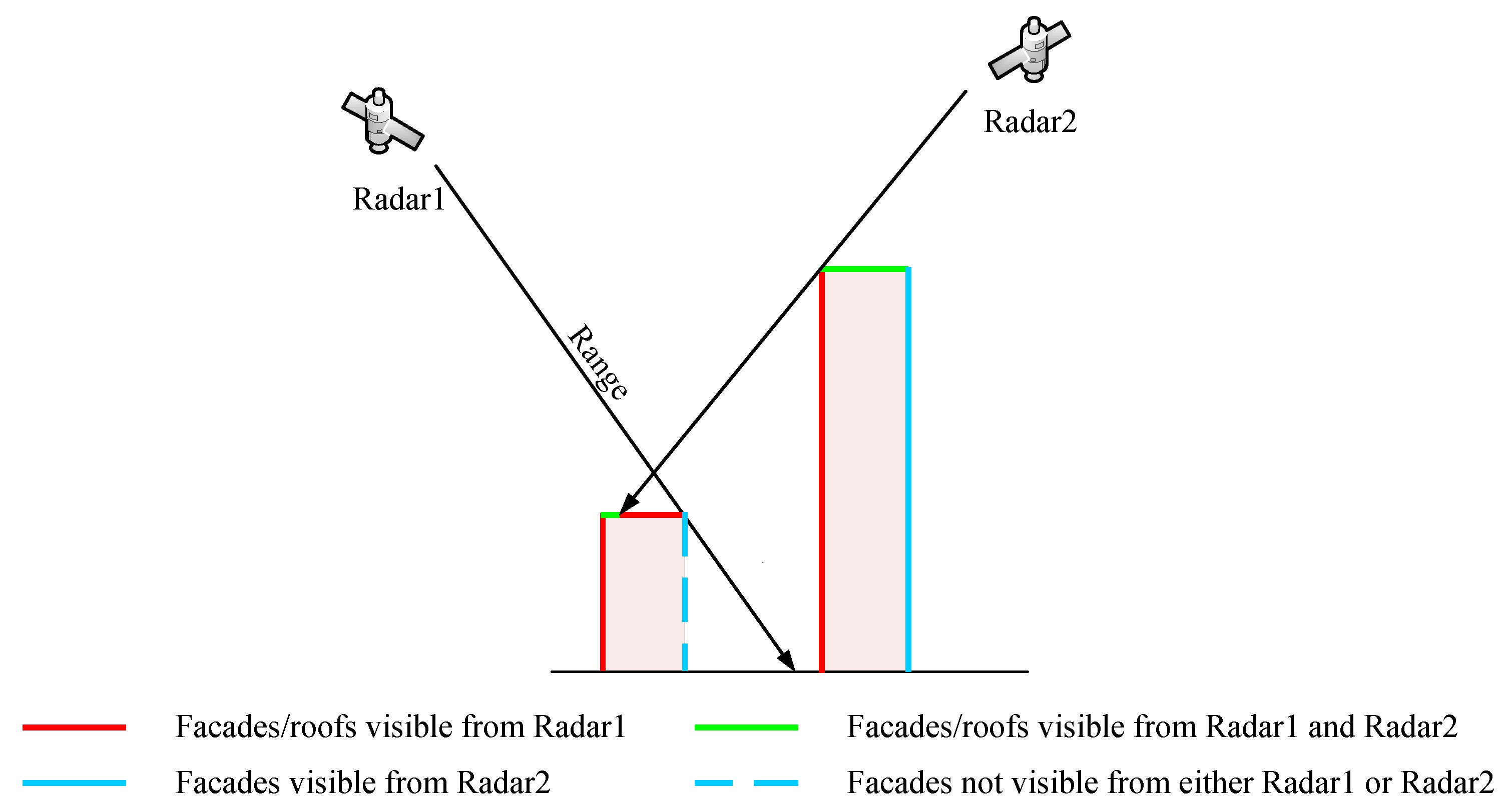
14]. Moreover, for the special combined buildings, occlusion cannot be completely solved by multi-view observation. As shown in
Figure 1, neither Radar1 nor Radar2 can obtain the direct waves of the lower building back. The other class is based on single-view TomoSAR. Shahzad et al. proposed a novel method that enables the reconstruction of the 2D/3D shapes of buildings by exploiting both facade points and roof points [
14]. For cases when no or very few facade points are available, the roof points are used to invert facades. Specifically, in this method, the boundaries of the extracted roof points can be equated to building footprints. Focusing on roof points and facade points, some high-precision or automatic methods under single-view TomoSAR have also been proposed [
15,
16]. Notwithstanding, the facade–roof fusion methods are very sensitive to the merits of the roof points. For cases with poor roof points, such as incomplete roof points due to occlusion, and even very sparse roof points due to weakly scattering roofs, the roof points may fail to reconstruct the backs of buildings with high precision. Consequently, these single-bounce-based methods are somewhat weak in reconstructing the backs of buildings.
Multipath scattering is an important phenomenon in the field of radar [
17,
18,
19]. The multipath distribution may reflect some specific structures of the observed objects, which is a complement to single-bounce scattering. The famous Terra-SAR image of Sydney Harbor Bridge released by DLR shows a rich multipath phenomenon [
9]. Numerous studies have been conducted on multipath interpretation in SAR images [
20,
21,
22]. The typical man-made objects, buildings, also have some interesting details caused by multipath scattering. For SAR images, Guida et al. developed an electromagnetic scattering model for the double-bounce scattering of buildings [
23]. By detecting the bright lines of double-bounce scattering at the facade–ground dihedral corner of buildings, the height information can be coarsely inverted [
24]. For the 3D TomoSAR point clouds, the points from multipath scattering can well be observed. Compared with the repeat-pass TomoSAR, airborne array TomoSAR can provide richer multipath points. Krieger et al. pointed out that there are two kinds of double-bounce scattering paths for array TomoSAR [
25,
26]. Zhang et al. discussed the double-bounce scattering phenomenon of the facade–ground dihedral corners [
27]. Moreover, the multipath scattering characteristics of cylindrical structures were given [
28]. However, in the studies mentioned above, the multipath scattering points are regarded as interference and are generally suppressed. In 2019, the double-bounce scattering model of dihedral corners was given [
29]. This model not only gives a good explanation for the distribution characteristics of the double-bounce scattering points, but also indicates that these points can be used for height estimation. Subsequently, triple and higher-order bounce scattering of the building dihedral corner structure was discussed and modeled [
30]. Nevertheless, these models only interpret the multipath scattering phenomenon between the illuminated facade of a single building and the ground. In fact, there are many densely distributed buildings in urban areas, and the interaction between buildings may cause a higher-order electromagnetic scattering phenomenon. For the backs of buildings, multipath may provide a new perspective on reconstruction.
Our team has been working on multipath interpretation and application research of airborne array TomoSAR [
27,
29,
30,
31]. In real point cloud processing, we found that the fourfold bounce (FB) scattering points between combined buildings are regularly distributed, and these points may imply information on the backs of buildings. In this paper, the FB scattering model for airborne array TomoSAR is demonstrated. Furthermore, a novel FB scattering point-based reconstruction method of building backs is proposed. The method consists of three main steps, including detection of the candidate FB scattering points, detection of FB scattering points, and reconstruction. First, the candidate FB scattering points are detected by performing a two-step constraint derived from the illuminated facades. Considering that the FB scattering points are vertically distributed in the elevation direction, region growing and density estimation are further performed for these detected points in the radar coordinate system. By thresholding, the detected points with higher density are considered as FB scattering points. Finally, the backs of buildings can be reconstructed by footprint inversion using FB scattering points. To verify the model and the effectiveness of the proposed method, the simulation experiments by means of ray tracing and two real airborne array TomoSAR flight experiments are presented. Moreover, two traditional roof point-based methods are selected for comparison.
This paper is organized as follows. In
Section 2, FB scattering between combined buildings in airborne array TomoSAR is analyzed in detail and modeled. In
Section 3, the proposed method is described in detail. In
Section 4, the processing results for both simulated data and real data are presented and quantitatively analyzed. As a comparison, the results of the traditional roof point-based methods are presented. Conclusions are given in
Section 5.
2. Model of FB Scatteing
In this section, the principle of airborne array TomoSAR is introduced firstly. Furthermore, the model of FB scattering is given.
2.1. Principle of Airborne Array TomoSAR
The airborne array TomoSAR allows multi-angle data acquisition in just one flight by arranging antennas in the cross-track direction [
7]. The 3D observation geometry of airborne array TomoSAR is described in
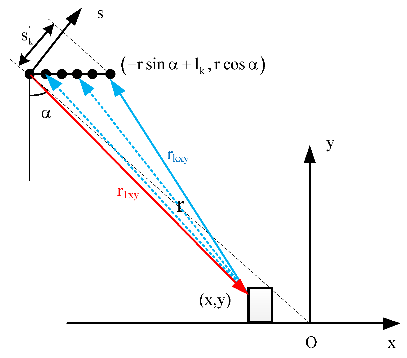
Figure 2. The antenna array is placed on the lower abdomen of the aircraft. For simplicity, the leftmost antenna is assumed to be the transmitting antenna (T) and all others are assumed to be the receiving antennas (R). Moreover, it is assumed that the system operates in side view and the phase centers of all the antennas lie in the zero Doppler plane. The schematic of airborne array TomoSAR on the ground–height plane is shown in
Figure 3.
According to the geometric relationship, the coordinates of the k-th receiving antenna in the plane can be denoted as , where r and are the range and the incidence angle formed by the leftmost antenna and the facade–ground dihedral corner of the building, respectively, and and are the horizontal baseline length and the effective baseline length of the kth antenna with respect to the leftmost antenna, respectively.
For scatterer
, the single-bounce scattering path of the
k-th antenna can be expressed as
Supposing that
,
, and
, the second-order Taylor expansion allows the above equation to be simplified to
where the first term represents the range, the second term is related to the flat phase and can be removed by phase compensation, and the third term represents the elevation. For simplicity, the second term is not considered in the following.
According to the TomoSAR model [
32], the single-bounce scattering path can also be written as
where the first term represents the range and
.
Therefore, the elevation can be expressed as
Consequently, based on the single-bounce scattering, airborne array TomoSAR can realize the elevation resolution of layover targets.
2.2. Distribution Pattern
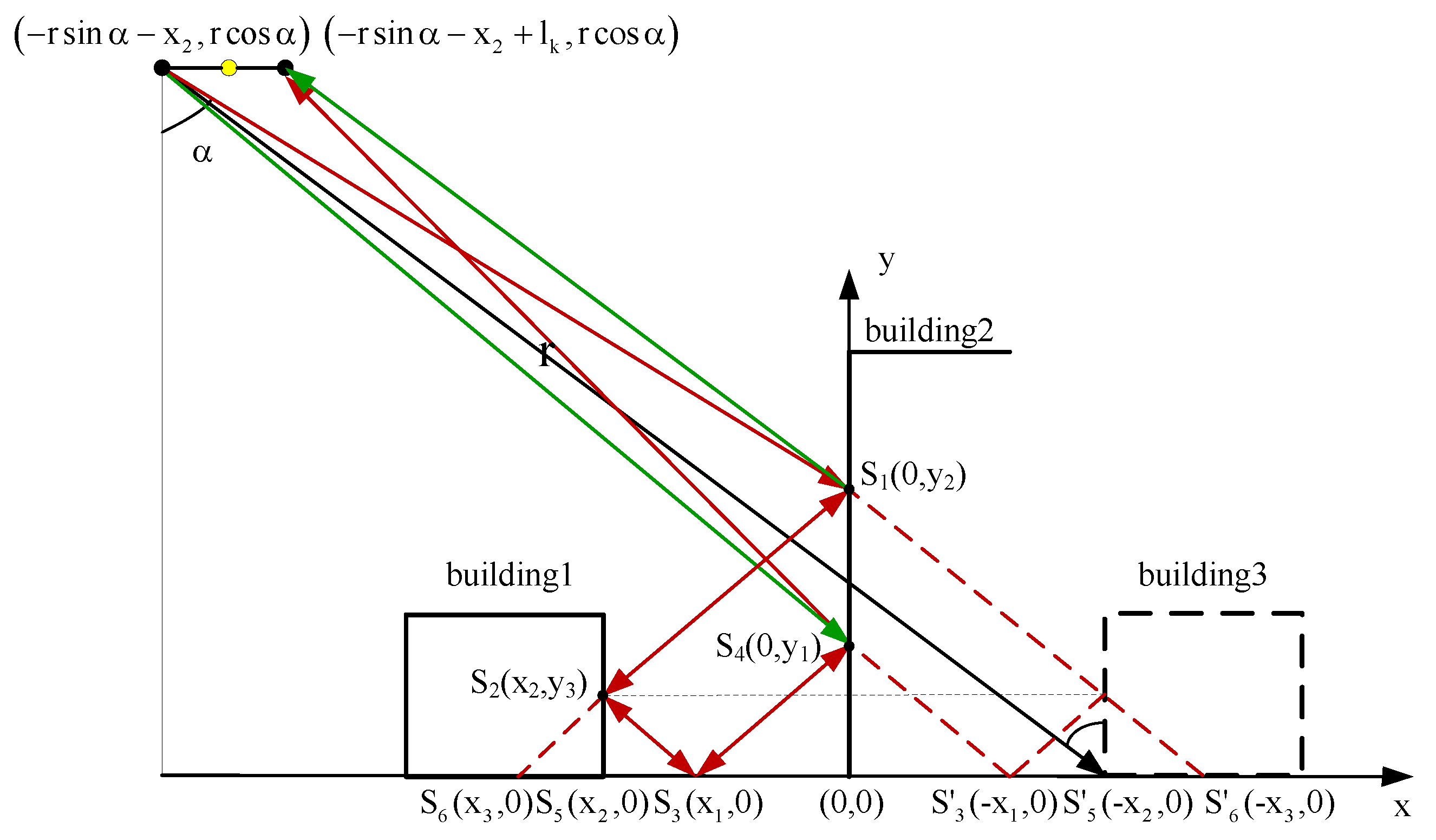
The schematic of FB scattering between combined buildings of airborne array TomoSAR is shown in
Figure 4. In this figure, building 1 and building 2 are real, and building 3 is a mirror image of building 1 with the facade of building 2 as the axis of symmetry. Due to the array mode, there are two paths of FB scattering through
and
(
).
Let the range and the incidence angle between the leftmost antenna and the facade–ground dihedral corner of building 3 be r and , respectively. Let the horizontal baseline length of the k-th antenna relative to the leftmost antenna be . Thus, the coordinates of the leftmost antenna on the x–y plane can be expressed as , and the coordinates of the k-th antenna can be expressed as .
The path length from the transmitting antenna to
is
The path length from
to the receiving antenna is
According to specular reflection, the path
equals
, where
and
are symmetrically distributed on both sides of the back of building 1. Moreover,
,
, and
are co-linear. The path length
can be expressed as
The path length
is
Similarly, the length of the first FB scattering path (
) after Taylor expansion is
For the other path, the path length from the transmitting antenna to
is
The path length from
to the
k-th receiving antenna is
Similarly, the path length of the other FB scattering (
) can be written as
According to specular reflection,
Therefore, the lengths of the two FB scattering paths can be approximated as
From Equation (
14), the range of the FB scattering through
and
is
r and the elevation is
. It can be concluded that the FB scattering between combined buildings can be equated to the double-bounce scattering at the facade–ground dihedral corner of the virtual building 3. As shown in
Figure 5, in the ground–height plane, the points from FB scattering are symmetrically distributed on both sides of the virtual corner with the range
r as the axis; in the range–elevation plane, the points from FB scattering are symmetrically distributed on both sides of the virtual corner of building 3 along the elevation direction. It is worth emphasizing that, different from the double-bounce scattering points symmetrically distributed in the facade–ground dihedral corner of real buildings [
30], the FB scattering points are located in the shadow area of building 2 and contain information about the back of building 1.
Only the combined buildings satisfying certain geometrical relationships are capable of FB scattering.
Figure 6 illustrates the distribution characteristics on the ground–height plane of array TomoSAR, where
indicates the ground value of the back of building 1,
and
indicate the height values of building 1 and building 2, respectively, and
indicates the incidence angle of the corner of building 3. In
Figure 6a,b, the relative ground distances between building 1 and building 2 are the same, and
. Only the influence of the relative building height on the distribution of FB scattering points is considered, and other possible cases will not be discussed in this paper.
As shown in
Figure 6,
, and
. FB scattering between combined buildings is found when and only when
. The intersection coordinate of the FB scattering line segment with the ground is
, and the coordinates of the upper and lower endpoints can be formulated as
and
, respectively.
L is the height of the back of building 1 that can be reached by FB scattering. As shown in
Figure 6a, when
,
L is determined by the height of building 2, i.e.,
. As shown in
Figure 6b, when
,
L is determined by the height of building 1, and reaches its maximum value, i.e.,
. Consequently, the FB scattering points are characterized as an oblique line segment on the ground–height plane. Similarly, they appear as a vertical line segment on the range–elevation plane. Although the relative building height affects the range of the FB scattering distribution, the intersection coordinate with the ground is unchanged and corresponds to the mirror image position of the back of building 1. Therefore, the distribution pattern of FB scattering between combined buildings can be expected to predict the position of the back of building 1.
3. Methods
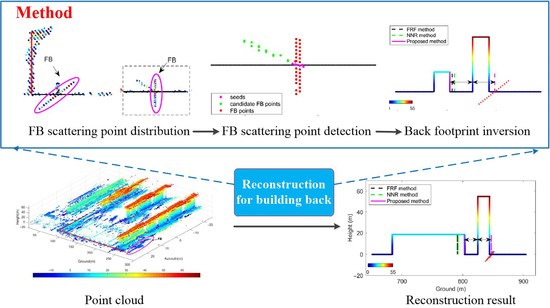
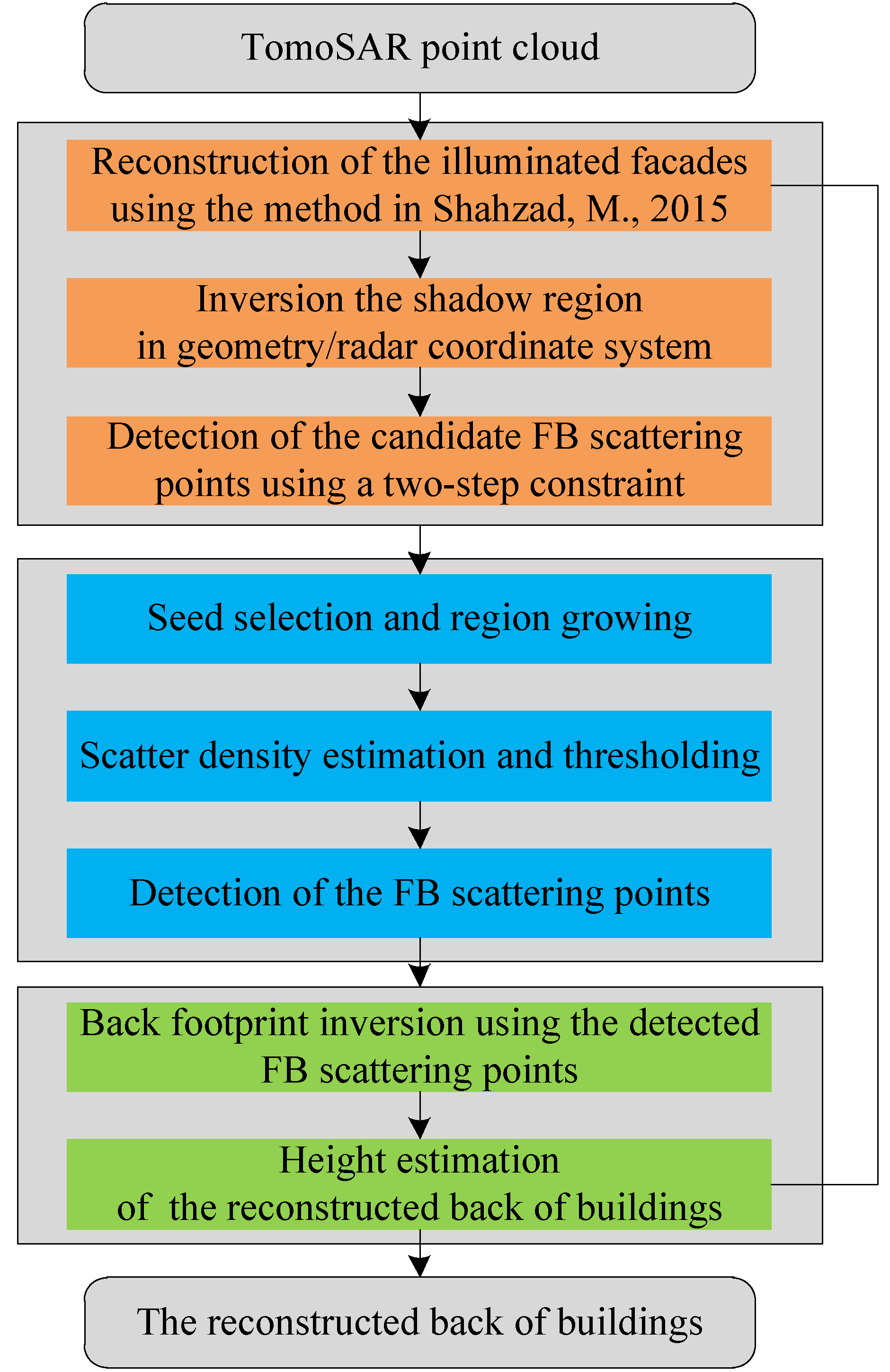
Figure 7 shows the workflow of the proposed method. The FB scattering points account for a small percentage of the point clouds. Moreover, there are many structures whose point density is much higher than the density of FB scattering points. If the detection of FB scattering points is performed in the entire point cloud space, the risk of error detection is extremely high. Based on the pattern that the FB scattering points are located in the shadow area of the illuminated facades, the whole processing begins by detecting the candidate FB scattering points. Then, a fine detection of FB scattering points will be performed in the radar coordinate system. This is because the FB scattering points are vertically distributed in the elevation direction. Similar to the assumption that the projection point density of the facades on the ground plane is higher, the high-density projection points in the azimuth–range plane can be helpful for detection. Finally, the detected points can be used to invert the back footprint of buildings. Furthermore, based on the assumption that the backs of buildings are vertical and have the same height as the corresponding illuminated facades, reconstruction can be performed.
The proposed method consists of three main steps, which will be described in detail below.
3.1. Detection of the Candidate FB Scattering Points
Facade reconstruction is usually the most important first step in building reconstruction. Many methods have been proposed and work well in the case of dense facade points. However, Shahzad et al. pointed out that there are cases when no or only a few facade points are available, particularly for the lower-height buildings. Therefore, a robust facade and point fusion method was proposed for facade reconstruction [
14]. For high-density facade points, the detection method using line fitting and surface normal vector analysis is used. First, the M-estimator is used for scattering point density estimation; then, a lower density threshold is set to retain the possible facade points; finally, the retained ground points and roof points are filtered out according to the normal vector difference of the facades and the roofs. For low-density facade points, the roof points will be extracted. Subsequently, its ground projection boundary will be equivalent to the facade footprint. The lower buildings in urban areas are easier to be sheltered, but cannot be ignored. Therefore, this method is applied to reconstruct the illuminated facades in this paper.
Let the vertex coordinate of the illuminated facade be
. Let the values in the ground direction and in the range direction at the near end of the shadow area be
and
, respectively, and the values at the far end be
and
, respectively. According to the geometry relationship, it can be derived that
After projection transformation,
where
is the incidence angle of the facade–ground corner and
.
Therefore, the candidate FB scattering points in the shadow area can be expressed as: .
By performing a two-step constraint, including both ground constraint and range constraint, the candidate FB scattering points in the shadow area can be detected.
3.2. Detection of the FB Scattering Points
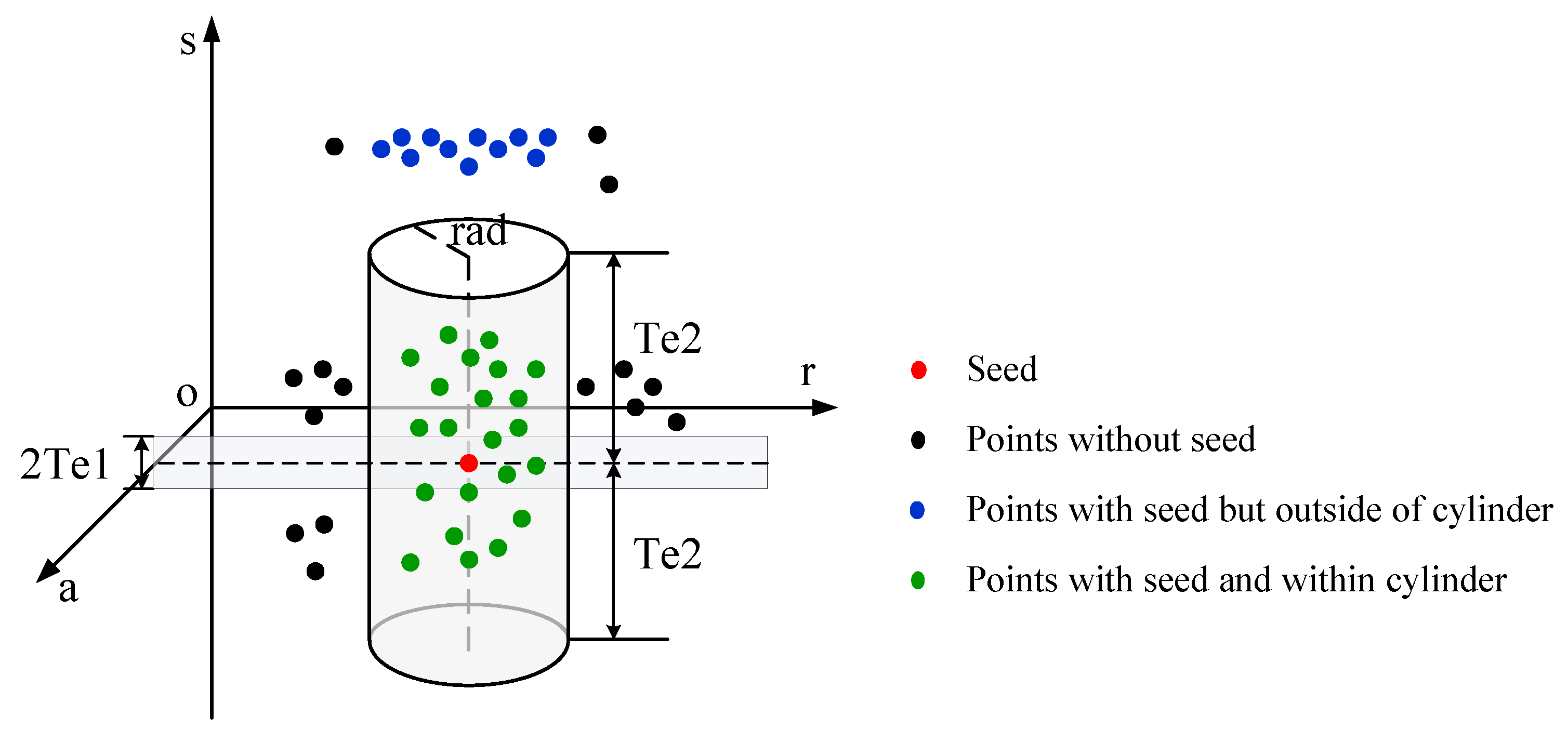
In the radar coordinate system, the FB scattering points are distributed vertically, which is consistent with the characteristic of the building facade being vertical to the ground plane in the geodetic coordinate system. Therefore, the scatter density can be used to detect the FB scattering points. In this step, the objects being processed are the candidate FB scattering points.
Figure 8 illustrates the FB scattering point detection in the radar coordinate system. Considering that the FB scattering points span the ground, the points with absolute elevation less than the threshold
will be regarded as seed points. Then, region growing [
33] is performed. For each seed, only the points that are located in the cylinder with radius
, height
, and centered on the seed point are considered as the neighboring points. This is because the distribution space of FB scatter points is limited, and the cylinder domain can further avoid the interference of possible interference points. Finally, the number of neighboring points for each seed is calculated. The seeds with density greater than the threshold
and their neighboring points are considered as the FB scattering points.
3.3. Reconstruction
In this step, the average range of the detected FB scattering points is calculated first. Then, the point whose elevation is 0 and whose range is the average range is projected into the geodetic coordinate system. The estimated value is the ground value of the corner of the mirror building 3, as mentioned before. Therefore, the mirror position of the ground value of the bottom corner of building 3 obtained on the axis of the reconstructed facade is the ground value of the reconstructed back. Finally, the vertical back whose height is the same as the height of the illuminated facade can be reconstructed.
4. Results
In this section, the results of the simulated data and real data are presented to validate the model of FB scattering and the proposed method. Specifically, we compare the facade–roof fusion (FRF) method [
14] and the neural network-based reconstruction (NNR) method [
16] to the proposed method.
4.1. Discussion on Parameter Selection
In order to strengthen the generality of the proposed method for real scenes, it is necessary to discuss in detail how to set the four key parameters in the step of FB scattering point detection, i.e., , , , and .
The parameter is the key parameter for seed point selection. While ensuring that the FB scattering points can be detected correctly, the smaller is, the fewer seed points are found and the fewer interference points are involved in the density estimation. Therefore, the optimal value can be expressed as , where is the minimum absolute elevation value of the FB scattering points. In this paper, it is set to 1 because the FB scattering point expands in the elevation direction from the position where the elevation value is 0. Since will be affected by data, it is set empirically and can also be scaled up appropriately based on the processed data.
The height threshold
has a clear physical meaning, i.e., the maximum absolute elevation value of the FB scattering points involved in density estimation. Larger values of
tend to mean that more FB scattering points are contained in the cylinder. On the other hand, setting
too large can introduce more interference points. As shown in
Figure 6b, the FB scattering points have a maximum value of
in the height direction; the value of
can be data-driven and its value can be calculated by
where
is the height of the reconstructed building 1,
is the unambiguous height of the TomoSAR system [
34], and
is the discrete number of points in a
elevation period [
35]. In order to adjust this parameter more flexibly, a positive constant factor
is also added. When it is less than 1, the constraint can be tightened, and vice versa, the constraint can be relaxed. It is recommended to take the factor
between 0.6 and 1.2, and it is set to 0.8 in this paper.
The parameter corresponds to the radius of the cylinder. Its optimal setting can not only ensure a good detection of the FB scattering points, but also can prevent the points with large deviations from the true FB scattering points in the range direction from participating in the range average estimation. Moreover, it is necessary to consider the range resolution, which should contain at least three range pixels. Because TomoSAR has high positioning accuracy in the range direction, it is set to 2 m in this paper.
The restrictions of seed and cylinder can almost avoid the influence of other high-density interference points. Therefore, the maximum density value of all seed points most likely corresponds to the density of FB scattering points. Nevertheless, the case where there are no or too few FB scattering points cannot be ignored. Consequently, the value of
is formulated as
where
is equal to the maximum density value of all seed points and is determined from the data,
is the allowable minimum density of FB scattering points, and
is the allowable minimum height of building 1. Only when the reconstructed scene satisfies the constraints in the first row, the detected points are considered as the FB scattering points; otherwise, the proposed method is not applicable to this kind of scene. In this paper,
is set to 30, and
is set to 5 m, which is also the minimum reconstructed building height in [
14].
In summary, and are empirical, and are set to 1 and 2 m in this paper; and are semi-empirical, and can be determined during the data processing in combination with the height of the reconstructed building 1 and scattering point distribution in different scenes. It should be noted that building 1 here represents the building closer to the radar direction among two combined buildings.
4.2. Simulation Experiments
4.2.1. Data Set
To illustrate the robustness of the proposed method to roof points, two scenes are simulated. The former is used to simulate a situation where the roof is fully illuminated, and the latter is used to simulate another situation where the roof is partially occluded. Moreover, the simulated combined buildings (building 1 and building 2) satisfy the geometric condition for the occurrence of FB scattering. The building 1 in scene 1 has a flat roof, and the coordinates of two opposite corners are (−5.0, 803.0, 20.0) m and (5.0, 787.0, 0.0) m. Besides an additional pointed roof, the building 1 in scene 2 is identical to the building 1 in scene 1. The horizontal inclination of the pointed roof is and the coordinates of the two endpoints of the roofline are (−5.0, 795.0, 26.0) m and (5.0, 795.0, 26.0) m, respectively. In addition, in both scenes, building 2 is a flat-roofed structure, and the coordinates of the opposite corners are (−5.0, 842.0, 55.0) m and (5.0, 826.0, 0.0) m, respectively. The dimensions of the coordinates indicate the azimuth direction, the ground direction, and the height direction in order.
POV-RAY is a feasible simulator for analyzing multipath scattering, which can not only simulate the geometric occlusion between the observed objects, but also can simulate specular reflection and diffuse reflection [
36,
37]. For this reason, POV-RAY is used to acquire the receiving points and the multipath information of the simulated scenes. The orthogonal projection camera is used to simulate the receiving channel and the parallel white light is used to simulate the transmitting channel. The camera position of both scenes is uniformly set to (0.0, 0.0, 1073.6) m, and both the camera irradiation origin and the light source irradiation origin are set to (0.0, 802.0, 0.0) m. Moreover, the light source is located at the same azimuth and height positions as the camera. The array TomoSAR system is simulated by only changing the position of the light source in the ground direction. The detailed parameters are shown in
Table 1. Eight antennas are uniformly distributed in the horizontal direction. The baseline interval is 0.084 m. The system works in
-band. After obtaining the multi-channel scattered point data, SAR imaging, image registration, point cloud generation [
35], and weak scattered point filtering will be executed. The discrete number of points in a
elevation period is 128. For an incidence angle of
, the unambiguous height of the simulation TomoSAR system is approximately 115 m.
Figure 9 presents the simulated scenes and the single-channel scattering points generated by POV-RAY. It can be seen that only the facades facing the radar direction have single-bounce scattering points. As a result, the backs of buildings are completely occluded. Additionally, the FB scattering points appear in the shadow area of building 2 and form a line segment with height 0.
4.2.2. Results
The parameters for FB scattering point detection are set:
,
m,
, and
is the maximum number of neighborhood points corresponding to all seed points. Among them,
and
are determined by Equations (
17) and (
18).
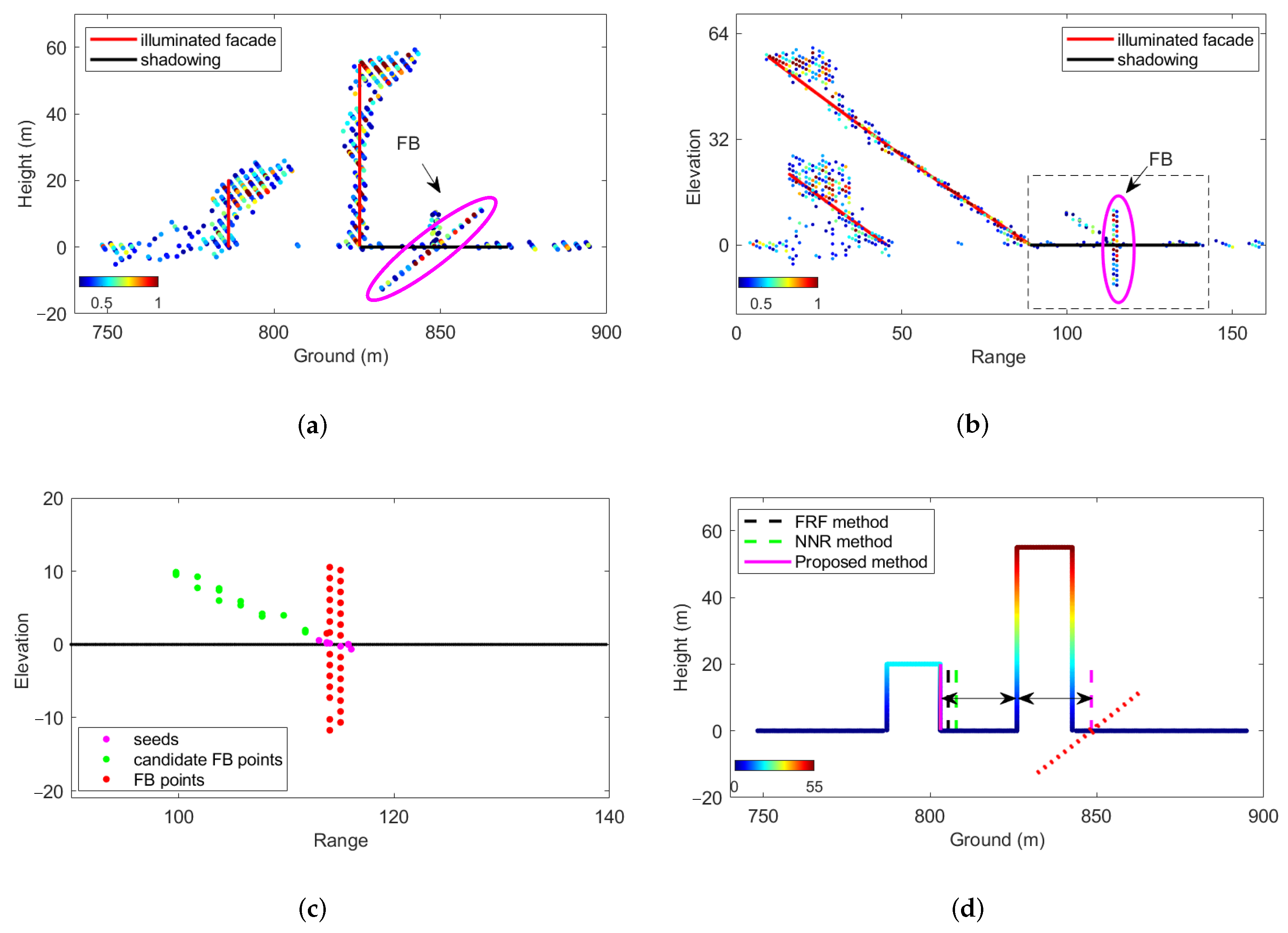
The whole reconstruction process of the back of building 1 in scene 1 is illustrated in
Figure 10. The TomoSAR point cloud and the candidate FB scattering point detection results are presented in the ground–height plane (
Figure 10a) and the range–elevation plane (
Figure 10b), respectively. Furthermore, the reconstructed illuminated facades are indicated by the red lines, the FB scattering points are contained in the purple ellipses, and the shadow area caused by the illuminated facade of building 2 is indicated by the black lines. Moreover, the black dashed rectangular box indicates the detected candidate FB scattering points under the two-step constraint. From
Figure 10a, it can be seen that the FB scattering points are symmetrically distributed on both sides of the ground plane along the height direction, presenting an oblique line segment. Meanwhile, these points are located within the ground range corresponding to the black line. It is worth emphasizing that the vertically distributed points behind building 2 are additionally added to simulate the high-density points that may appear in real data. From
Figure 10b, it can be seen that the FB scattering points are vertically distributed in the elevation direction. Therefore, the FB scattering points will have higher density in the azimuth–range projection plane. However, roof points can also be detected using only the ground constraint. These high-density roof points may lead to incorrect detection of FB scattering points. Combing the range constraint, these points outside the range can be well removed. The detection of FB scattering points in the range–elevation plane is illustrated in
Figure 10c. It can be seen that the FB scattering points can be extracted by seed selection and high-density scattering point detection. For candidate FB scattering points without corresponding seed points, they will not participate in the density estimation even if they have a high density. Finally, as shown in
Figure 10d, the reconstruction results indicate that the proposed method outperforms the traditional methods and almost overlap with the true value.
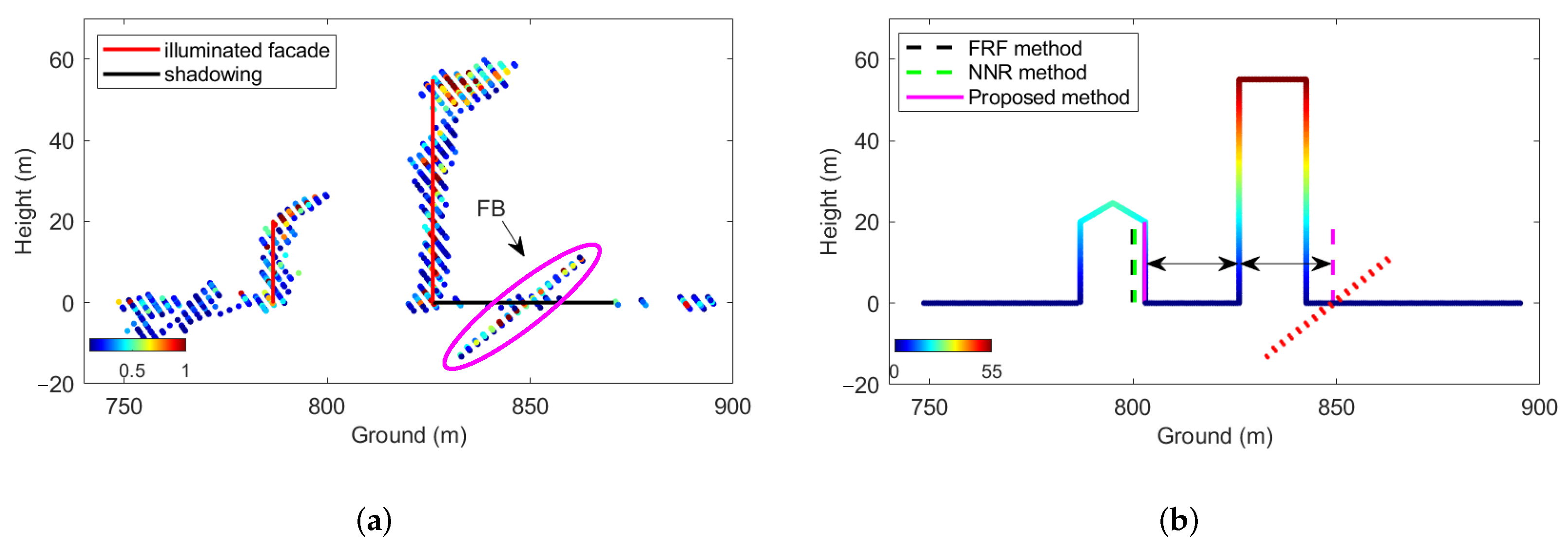
Figure 11 presents the TomoSAR point cloud and the reconstruction results of the back of building 1 in scene 2. From
Figure 11a, the points on the weakly scattered back slope of the pointed roof have been completely filtered out. Moreover, the FB scattering points appear as an oblique line segment that is symmetrically distributed along the height direction on both sides of the ground.
Figure 11b presents the reconstruction results of the back of building 1. It can be seen that the proposed method is more robust to the roof points than the traditional methods. Furthermore, the proposed method can correctly detect the FB scattering points, and the reconstruction result is closer to the true value.
The reconstruction performance of the back of building 1 in the simulation experiments is quantified in
Table 2. Since the focus of the proposed method is to reconstruct the backs of the buildings, whose back information is implied in the FB scattering points, the evaluation of building 2 is not given. In both scenes, the true value of the back of building 1 in the ground direction is 803.00 m and the width of its roof is 16.00 m. For the back of building 1 with a flat roof, the results of the FRF method, the NNR method, and the proposed method are 805.58 m, 807.80 m, and 803.16 m, respectively. The absolute errors are 2.58 m, 4.80 m, and 0.16 m, respectively. For the back of building 1 with a pointed roof, the results of the three methods are 799.90 m, 800.40 m, and 802.85 m. The absolute errors are 3.1 m, 2.60 m, and 0.15 m, respectively. It can be seen that the accuracy of our method is better than that of the traditional methods. Moreover, it is almost independent of the roof point quality of the reconstructed building 1.
It is worth noting that the ray-tracing scattering coefficient does not exactly match the real situation. Moreover, the double-bounce scattering and the triple-bounce scattering that may exist in the real situation are not considered in the simulation experiment. In addition, the simulated buildings do not have structures such as windows. Although the scattering coefficient of the roof is stronger than that of the facades (e.g.,
Figure 9c), it does not affect the reliability of the simulation experiment. This is because the strongly scattered roof intentionally enhances the performance of the traditional method based on the roof boundary. Similarly, the TomoSAR point cloud of the pointed roof in scene 2 is not the worst case when the backside roof is completely obscured. Therefore, in the two simulated scenes, the roof scattering is relatively ideal. Nevertheless, the proposed method outperforms the traditional methods. To sum up, it is reasonable to deduce that the advantage of the proposed method can be more significant in worse roof scattering cases.
4.3. Real Experiments
4.3.1. Data Set
In 2014, our team conducted an airborne array TomoSAR flight experiment in Yuncheng, Shanxi Province, China. It is referred to as Experiment 1 below. The system works in
-band, and operates in right-side view. The aircraft flies from east to west. Eight antennas are arranged in the cross-track direction with a baseline interval of 0.084 m. In addition, our team conducted an airborne array TomoSAR flight experiment in Leshan, Sichuan Province, China in 2019. In the following, it is referred to as Experiment 2. The system works in
X-band and operates in left-side view. The flight heading is from west to east. Twelve antennas are horizontally arranged in the cross-track direction. For an incidence angle of
, the system unambiguous heights of Experiment 1 and Experiment 2 are approximately 115 m and 140 m, respectively. The specific experimental parameters are shown in
Table 3.
In the following, the processing results and analysis of the two experiments will be presented.
4.3.2. Results of Experiment 1
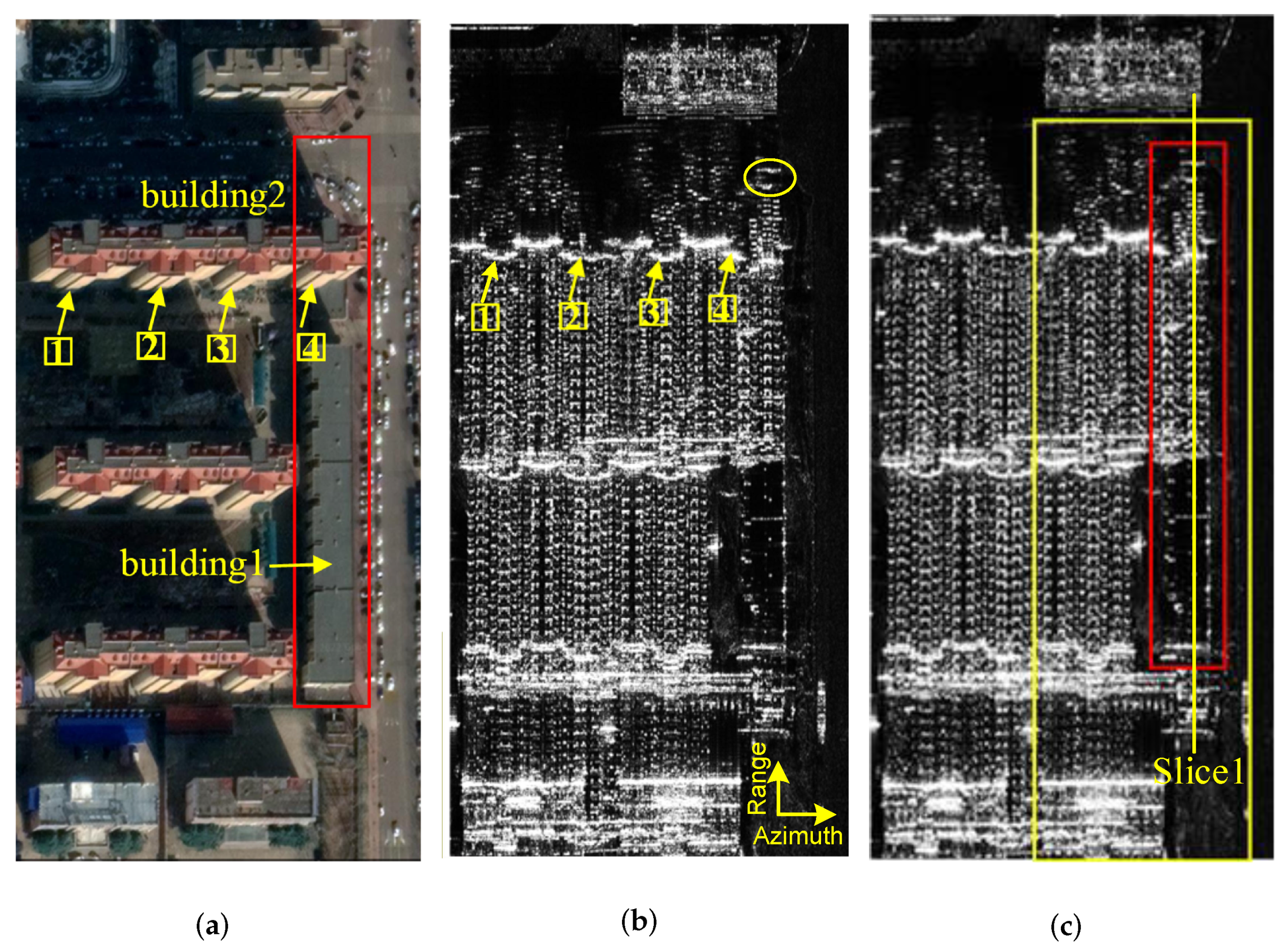
The optical image and SAR images of the studied scene are shown in
Figure 12. The SAR images are matched with the optical image, where the yellow rectangular boxes labeled 1, 2, 3, and 4 correspond to the bottom corner of the raised facade of building 2. The high scattering intensity is caused by double-bounce scattering. The red rectangular box shows building 1 and building 2, which overlaps with building 1 in the azimuth direction. As can be seen from the optical image, the back of building 1 is flat. Within the red rectangle, the scene behind building 2 is relatively clean. However, in the SAR images, some pixel points with strong scattering intensity, such as the yellow ellipse box in SAR image 1, appear behind building 2. In order to interpret the phenomenon more intuitively,
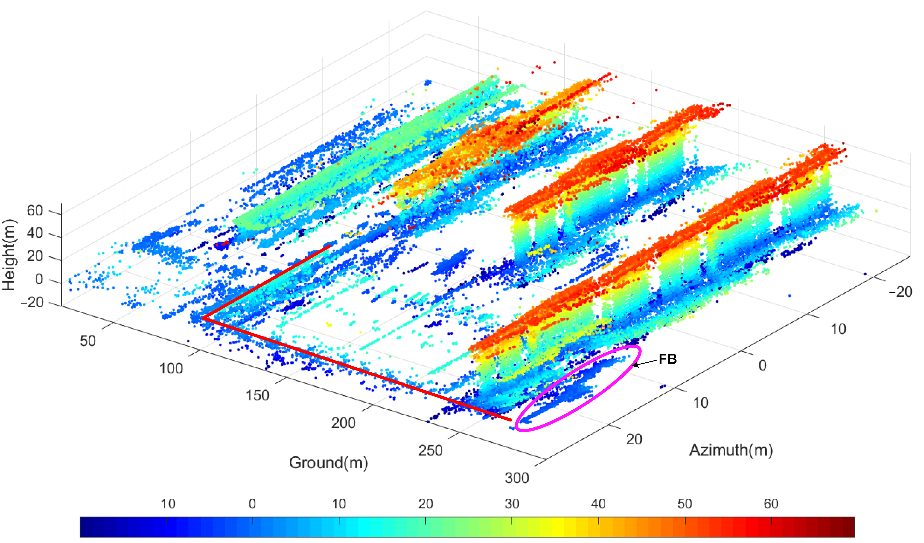
Figure 13 presents the original TomoSAR point cloud of the area marked by the yellow rectangular box in SAR image 2. These strong points in the SAR images are within the purple ellipse. It can be seen that these points are dense, and they are distributed almost symmetrically on both sides of the ground. Furthermore, according to the illumination geometry and the aforementioned distribution pattern of FB scattering points, these points that should have been obscured are caused by FB scattering between building 1 and building 2.
Figure 14 presents the TomoSAR point cloud and the reconstruction results of the back of building 1 in Slice 1. The parameters for FB scattering point detection are the same as those of the simulation experiments. As shown in
Figure 14a, the scattering intensity of the roof points of building 1 is weaker than that of the facade points. The roof points of building 1 are very sparse in the TomoSAR point cloud. In addition, the purple ellipse contains FB scattering points, which are symmetrically distributed along the height direction. The back reconstruction results are presented in
Figure 14b. The black dashed line and the green dashed line indicate the results of the FRF method and the NNR method, respectively. Here, it is assumed that all roof points can be detected to intentionally improve the performance of the traditional methods. In fact, some sparse roof points will be ignored with a high probability. It can be seen that the reconstructed back of building 1 by the mirror inversion of FB scattering points (marked by the solid purple line) is closer to the true value. Furthermore, the measured roof width of building 1 is 118 m. Assuming that there is no error of the reconstructed illuminated facades in the ground direction, the true value for the back of building 1 is 803.06 m. Since the back of building 2 is not the concern of this paper, the roof width obtained by the FRF method is taken as the true value to obtain a better display effect. The ground values obtained by the traditional FRF method, the NNR method, and the proposed method are 791.28 m, 791.90 m, and 802.42 m, respectively. The absolute errors relative to the true value are 12.32 m, 11.70 m, and 1.18 m, respectively. Consequently, for building 1 with very sparse roof points, the proposed method is closer to the true value, and the accuracy can be improved to 1.18 m.
4.3.3. Results of Experiment 2
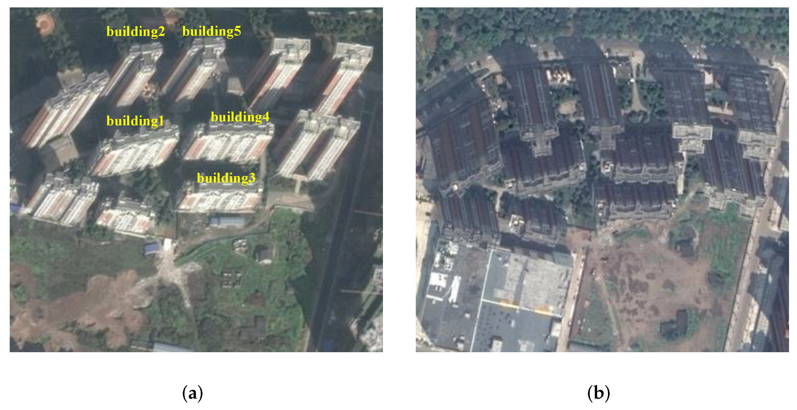
The optical image of the studied scene is shown in
Figure 15. In this community, building 1 and building 2, building 2 and building 3, and building 4 and building 5 satisfy the FB scatter condition. According to the SAR image shown in
Figure 16, it can be seen that Slice 1 contains building 1 and building 2, and Slice 2 contains buildings 3–5. Therefore, the processing results of the two slices will be presented in detail.
For Slice 1, the TomoSAR point cloud and the reconstruction results of the back of building 1 are presented in
Figure 17. From the TomoSAR point cloud, it can be seen that there are some interference points and FB scattering points in the shadow area of builiding 2. Among them, the FB scattering points are consistent with the FB scattering distribution pattern. From the reconstruction results, all three methods can reconstruct the back of building 1. However, due to the different reconstruction ideas, the two traditional roof point-based methods deviate greatly from the reference true value, while the reconstruction result of the proposed method is closer to the reference true value.
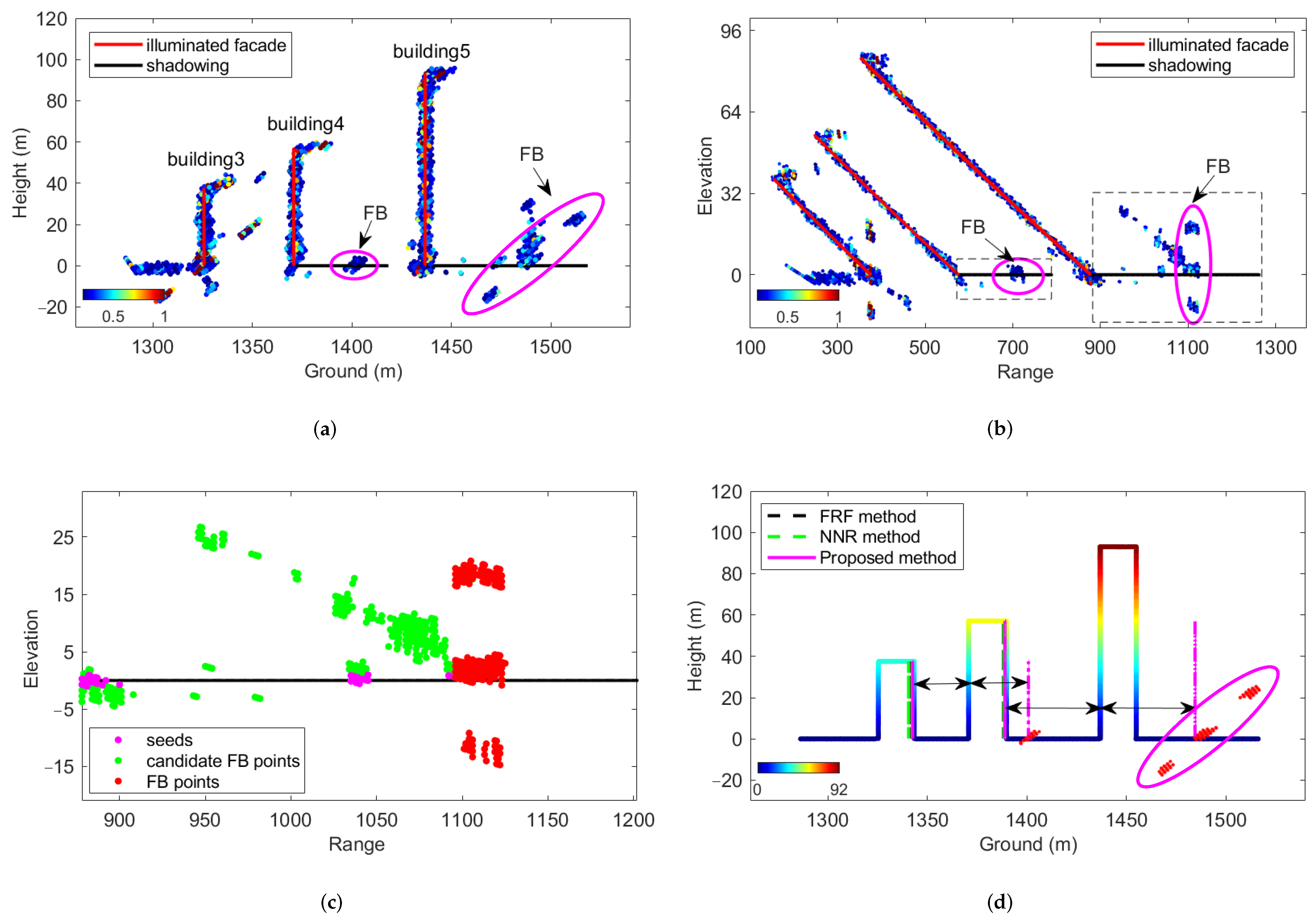
Since three buildings are included in Slice 2,
Figure 18 illustrates the whole reconstruction process. This is more beneficial to verify the FB scattering distribution pattern and the proposed method. From
Figure 18a,b, it can be seen that the FB scattering points from building 3 and building 4 are located in the shadow area of building 4, and the FB scattering points from building 4 and building 5 are located in the shadow area of building 5. Moreover, the distribution of these FB scattering points is consistent with the theoretical analysis. The candidate FB scattering points are in the black rectangular boxes in
Figure 18b. It can be seen that performing ground and range constraints can be effective in avoiding interference. Taking the candidate FB scattering point detection in the left dotted rectangular box as an example, if the ground constraint is used alone, the roof points of building 4 will be misidentified as the candidate FB scattering points; if the range constraint is used alone, the facade points of building 5 within the range will be misidentified as the candidate FB scattering points.
Figure 18c presents the detection results of the FB scattering points for the candidate FB scattering points inside the right dotted black rectangular box. First, by setting the parameter
(equal to 1), the FB scattering points will participate in the density estimation, while most of the interference points do not have seed points and do not participate in the density estimation. Then, by setting the parameters
(equal to 2 m, around 26 range units) and calculating the parameter
(equal to 32), the FB scattering points all fall within a cylinder. Moreover, the maximum density of all seeds is equal to 1119, and the height of the reconstructed building 4 is higher than 5 m. Consequently,
, and the FB scattering points are detected. Finally, the reconstruction results are presented in
Figure 18d. The reconstruction results of the three methods are similar, and all are close to the reference true value.
The reconstruction performance is quantified in
Table 4. First, the acquisition of the reference true value is introduced. It can be seen from the optical image in
Figure 15 that the roof structures of building 1, building 3, and building 4 are the same. Moreover, their roofs are relatively flat, and do not belong to the pointed roofs that may be shaded. Therefore, by averaging the nine roof widths of the three buildings reconstructed by the three methods, the true value of the roof width is around 18 m. Since building 2 and building 5 are not the concern of this paper, their roof widths are also 18 m by default. Furthermore, assuming that there is no error of the reconstructed facades, the reference true values in the ground direction of the back of building 1, the back of building 3, and the back of building 4 are 1413.00 m, 1343.30 m, and 1389.70 m, respectively. Next, the results of the three methods for the same building are compared cross-sectionally. The accuracy of the two methods, FRF and NNR, is similar, not exceeding 0.5 m. This is because they use the same data input and the same idea for the back reconstruction. This smaller variability is due to the fact that the NNR method first fits the input data and then inverses the building backs. Due to the different reconstruction ideas, the accuracy of the proposed method is not completely consistent with the traditional methods. When the reconstruction error of the traditional methods for building 1 is as high as 5 m, the error of our method is 1.39 m. Then, the effects of different data on the same method are compared longitudinally. It can be seen that the two traditional methods are sensitive to the quality of the roof points, while the proposed method is robust to the quality of roof points. It should be noted that although there may be errors in the reference true value, such deviations are consistent for all buildings and do not affect the reasonableness of the above analysis. Meanwhile, combining the processing results of simulation and Experiment 1, it can be concluded that the accuracy of the proposed method and the traditional methods is close in the case of good quality of roof points; for the case of poor quality of roof points, our method can maintain robust reconstruction.
5. Conclusions
The traditional methods for reconstructing the backs of buildings using TomoSAR point clouds only consider the single-bounce scattering, which makes its accuracy very sensitive to the merits of the single-bounce scattering points. To overcome the problem, this paper focuses on the FB scattering-based reconstruction of building backs using airborne array TomoSAR point clouds. First, the FB scattering model in array TomoSAR is derived. Furthermore, the distribution pattern and critical conditions of the FB scattering points are given. This is not only helpful for point cloud interpretation, but also provides a new perspective for the reconstruction of building backs. Taking full advantage of the pattern that the FB scattering points are vertically distributed along the elevation in the shadow region, a novel FB scattering-based method for reconstructing building backs is proposed. The effectiveness is validated via ray-tracing simulation results and airborne array TomoSAR experimental results. Compared with the traditional roof point-based methods, the proposed method allows high-precision reconstruction, even in the case of poor points. To sum up, the proposed method is applicable to reconstruct the backs of buildings closer to the radar direction in combined buildings where FB scattering can occur, which facilitates high-precision 3D reconstruction in dense urban areas.
However, several aspects of our work can be improved upon. First, our work still belongs to the principle and feasibility verification of the proposed method. Second, the reconstructed backs are smooth. In fact, for backs with structures such as windows, FB scattering may also provide richer structural information. In the future, more work will focus on large-scale data verification and the back reconstruction of complex structures.


 ,
, 


