Article

Investigating the Potential of Sentinel-2 MSI in Early Crop Identification in Northeast China

1
Aerospace Information Research Institute, Chinese Academy of Sciences, Beijing 100094, China
2
University of Chinese Academy of Sciences, Beijing 100049, China
*
Author to whom correspondence should be addressed.
Remote Sens. 2022, 14(8), 1928; https://doi.org/10.3390/rs14081928
Submission received: 12 March 2022 / Revised: 13 April 2022 / Accepted: 13 April 2022 / Published: 15 April 2022

Abstract

:
Early crop identification can provide timely and valuable information for agricultural planting management departments to make reasonable and correct decisions. At present, there is still a lack of systematic summary and analysis on how to obtain real-time samples in the early stage, what the optimal feature sets are, and what level of crop identification accuracy can be achieved at different stages. First, this study generated training samples with the help of historical crop maps in 2019 and remote sensing images in 2020. Then, a feature optimization method was used to obtain the optimal features in different stages. Finally, the differences of the four classifiers in identifying crops and the variation characteristics of crop identification accuracy at different stages were analyzed. These experiments were conducted at three sites in Heilongjiang Province to evaluate the reliability of the results. The results showed that the earliest identification time of corn can be obtained in early July (the seven leaves period) with an identification accuracy up to 86%. In the early stages, its accuracy was 40~79%, which was low, and could not reach the satisfied accuracy requirements. In the middle stages, a satisfactory recognition accuracy could be achieved, and its recognition accuracy was 79~100%. The late stage had a higher recognition accuracy, which was 90~100%. The accuracy of soybeans at each stage was similar to that of corn, and the earliest identification time of soybeans could also be obtained in early July (the blooming period) with an identification accuracy up to 87%. Its accuracy in the early growth stage was 35~71%; in the middle stage, it was 69~100%; and in the late stage, it was 92~100%. Unlike corn and soybeans, the earliest identification time of rice could be obtained at the end of April (the flooding period) with an identification accuracy up to 86%. In the early stage, its accuracy was 58~100%; in the middle stage, its accuracy was 93~100%; and in the late stage, its accuracy was 96~100%. In terms of crop identification accuracy in the whole growth stage, GBDT and RF performed better than other classifiers in our three study areas. This study systematically investigated the potential of early crop recognition in Northeast China, and the results are helpful for relevant applications and decision making of crop recognition in different crop growth stages.

1. Introduction

Crop identification and preliminary estimation of crop planting areas in the early stage can provide valuable and timely information for individual farmers regarding farmland management, agricultural insurance, and agricultural subsidy policies. It is also of great significance for agricultural management departments to make reasonable decisions [1,2,3]. Remote sensing technology can map the latest and most detailed crop-type mapping in a timely and accurate manner, which has been proven to be one of the most effective means for obtaining precise crop information [4,5,6,7].
At present, using remote sensing technology to identify crops is mainly focused on the middle or late stage of crop growth [8,9,10], and early crop recognition refers to identifying crops as early as possible from crop emergence to preharvest [9,10,11,12]. The crop information is too weak at this time, compared with the middle or late stage [10,11,12]. Moreover, the ground sample work has not been collected. Therefore, the sample problem is one of the challenges faced by early identification. All of these factors have resulted in a relatively few studies on early identification. Although many challenges make early-stage crop recognition difficult, previous studies have attempted to solve these problems with different methods. It can be divided into the following two methods: (1) Using the key features in the key phenological periods. For example, during the transplanting period of rice, there is often 2–15 cm water in the paddy field, and the surface is a mixture of rice and water. Based on this a priori knowledge, Wei et al. [13] used the Land Surface Water Index (LSWI) threshold method to realize rice identification in the transplanting period. Wang et al. [14] used multi-temporal images of winter wheat, including the periods of sowing, seedling emergence, tillering, and wintering, and then took the multi-scale segmentation object as the basic classification unit. Finally, the early recognition of winter wheat was realized by constructing a hierarchical decision threshold. However, the above-mentioned studies identified crops by constructing decision thresholds according to the different spectral characteristics of ground objects in the key periods, and the determination of threshold value was both time consuming and laborious. Thus, the efficiency of automatic crop extraction was greatly reduced. Furthermore, the determination of the same crop’s threshold was difficult to apply to other regions due to the influence of soil, vegetation type, and image brightness [15,16,17,18,19]. (2) Using the image data or ground survey data in historical years. This type of method learned knowledge from historical year data and applied to the target year with the help of transfer learning technology. You et al. [20] trained the classifier by using the early season image time series and field samples collected in 2017, and then the classifier was migrated to the corresponding time series image data of the target year in 2018 to realize the early recognition of crops. In this paper, a single binary classifier (target ground object and non-target ground object) was trained for the recognition of each crop, but when there were many target objects to extract, the method was time-consuming. Vorobiova et al. [21] used historical data and the cubic spline function to generate Normalized Difference Vegetation Index (NDVI) time series to realize early crop recognition in the current year. However, they only considered a single NDVI in their study, and the inversion information of a single index was limited, so the identification accuracy of crops had some constraints [22,23,24,25,26].
All the above studies demonstrated that remote sensing technology has the potential to identify crops in the early stage; however, they placed too much focus on a single crop type, and the features used in their studies were relatively few. All of them lacked a systematic summary and research on how to obtain training samples quickly in the early stage, how early different crops can achieve a satisfactory level of monitoring accuracy, and what are the key identification features used to achieve crop identification, as well as what accuracy level each stage can achieve. So, it is difficult to obtain a comprehensive answer to the above questions.
Therefore, our objectives are: (i) Explore the feasibility of the sample automatic generation method based on the historical crop maps and image remote sensing images; (ii) Summarize and analyze the optimal features in different stages; (iii) Explore how early crops can be identified, what the accuracy variation characteristics of crops at different stages are, and the differences among different classifiers. Specifically, first, the automatic sample generation method was used to obtain the training samples based on the historical crop maps from 2019 and remote sensing images from 2020. Second, the feature optimization method was used to calculate feature importance. Therefore, the optimal feature sets in different stages can be achieved. Third, four classifiers were used to identify crops in different periods. Through the above three parts, the potential of early-stage crop recognition in Northeast China are systematically explored.

2. Study Area and Data
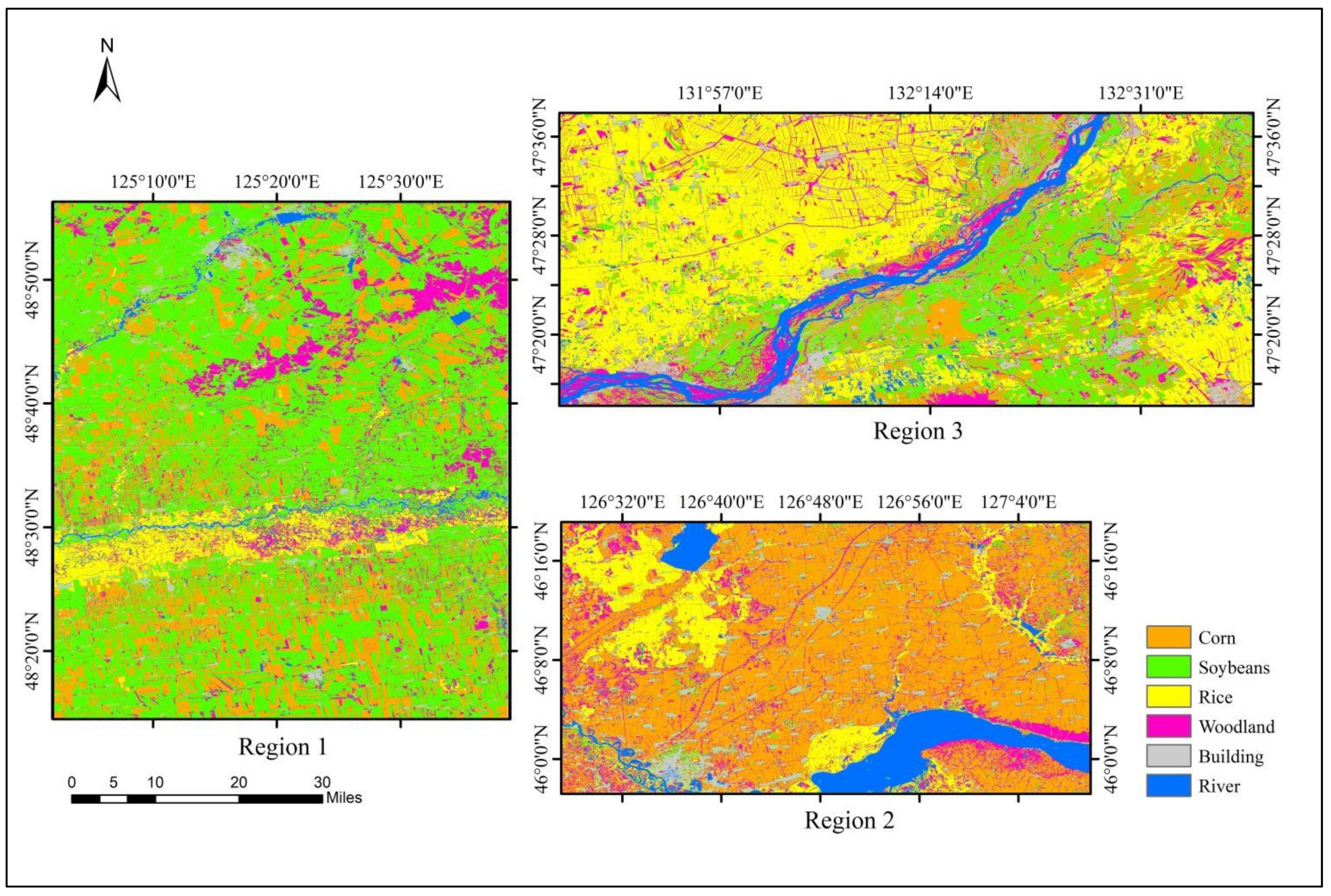
2.1. Study Area

Heilongjiang is an important commodity grain base in China. Three typical study areas with different characteristics were selected in Heilongjiang (Figure 1) as our study areas. They basically included the main crop types combinations of bulk crops in Heilongjiang, which provided good conditions for the extrapolation of research methods and the objectivity of research conclusions.
Region 1 (125°02′ E–127°64′ E, 48°24′ N–48°94′ N) is located on the Songnen Plain. The crop planting structure in Region 1 is relatively complex and fragmented, with intercropped corn and soybeans being the major crops in this region. Rice is mainly distributed along the river.
Region 2 (126°45′ E–27°16′ E, 45°95′ N–46°31′ N) is also located on the Songnen Plain, the crops in this area are mainly corn, followed by rice, and soybeans are planted sparsely.
Region 3 (131°67′ E–132°72′ E, 47°23′ N–47°63′ N) is located on the Sanjiang Plain. The region’s major crop is rice, followed by corn and soybeans, and both of them are covered with large areas. In the western part of the region, some soybeans and corn are around rice.
The three crops are harvested only once per year due to low sunshine hours and accumulated heat. Their growing seasons are concentrated from April to early October, and all of them are sown in April. At this time, the water information on rice is more prominent in the image, whereas the corn and soybeans are in the state of bare land. In the early June, the rice is in the reviving period, and it is a mixture of water and rice in the image. Corn and soybeans are in the seedling period and show low vegetation. From July to August, the crops gradually enter vigorous growth, and the spectral characteristics of each crop are more obvious with a certain degree of separability in the image. In the September to early October, all crops gradually enter the mature and harvest period, soybeans are harvested first, followed by corn, and rice is harvested in early October. Based on the performance of different crops in all the available images, we divided the entire growth stage into three stages: the early stage (April–June), the middle stage (July–August), and the late stage (September–early October). These crops show different characteristics in different growth stages, and the crop types can be identified as early as possible according to these key characteristics [20].

2.2. Data

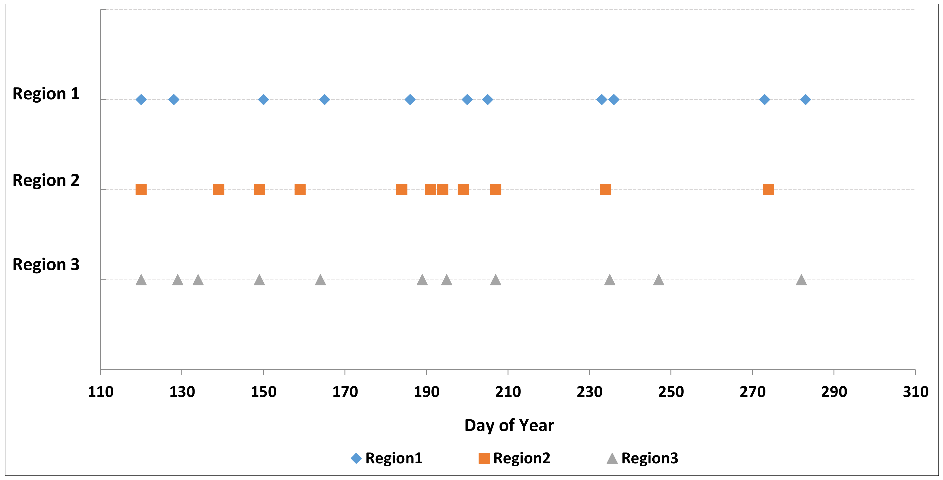
2.2.1. Sentinel-2 Data

Sentinel-2 is equipped with the state-of-the-art Multi-Spectral Instrument (MSI), whose revisit period is 2–5 days depending on latitude, and the width is 290 km. It can provide optical images with a minimum resolution of 10 m, and the spectral bands cover 13 bands from visible light, near-infrared, red-edge to shortwave infrared (Table 1). Sentinel-2 has been proven to be an effective means of monitoring different crop types [27,28,29,30,31]. The Google Earth Engine (GEE) cloud platform provides an efficient environment to process Sentinel-2 data and can effectively implement various satellite-based remote sensing applications and research activities. The Sentinel-2 dataset in this platform contains completed data preprocessing work, such as radiometric calibration, terrain correction, and geometric correction. The pre-processing work we performed included selecting the images with cloud cover less than 10% from April to early October in 2020, and using Q60A band to remove thick clouds in some images. In addition, image cutting work was also necessary.
The availability of useful data is limited due to clouds. Therefore, 34 good quality images in 2020 that could cover our study areas (Figure 2) were selected. Among them, 11, 11, and 12 images were used in Region 1, 2, and 3, respectively. The cloud coverage of these images was less than 10%, which could meet the monitoring requirements. The images collected in each study area can generally cover the period from crop sowing to harvest, which facilitates the objective results of the identification features and identification capabilities of each stage. Previous studies have shown that the use of single-date remote sensing images have limited crop identification accuracy in the early stage, and combining multi-date images can effectively improve the crop identification accuracy [3,20]. Therefore, some incremental designs were made for the available image used in each period. That is, when performing a supervised classification, every time that the image was used in a current period, all the previously available images also needed to be included. Finally, there were 11, 11, and 12 periods for image-conducted increment designs in Region 1, Region 2, and Region 3, respectively. From the accuracy obtained at different periods in each study area, we explored how early can the crops be monitored, and what level of accuracy can crops achieve at different stages.

2.2.2. Ground Survey Data

The ground samples are difficult to obtain in the early stage of crops. To reasonably and effectively evaluate the reliability of the training samples generated based on historical crop maps from 2019 and remote sensing images from 2020. The ground survey data were only used as validation samples to evaluate the classification results in our study. The Songnen Plain and Sanjiang Plain are our major ground survey areas. Rice, corn, and soybeans are major crops in these areas, so the latitude and longitude of these crops we collected were labeled, and the samples of woodlands, buildings, and rivers were labeled by combining Google Earth and Sentinel-2 images with visual interpretation. The usage of sample points in each study area is shown in Table 2.

2.2.3. Supplementary Data
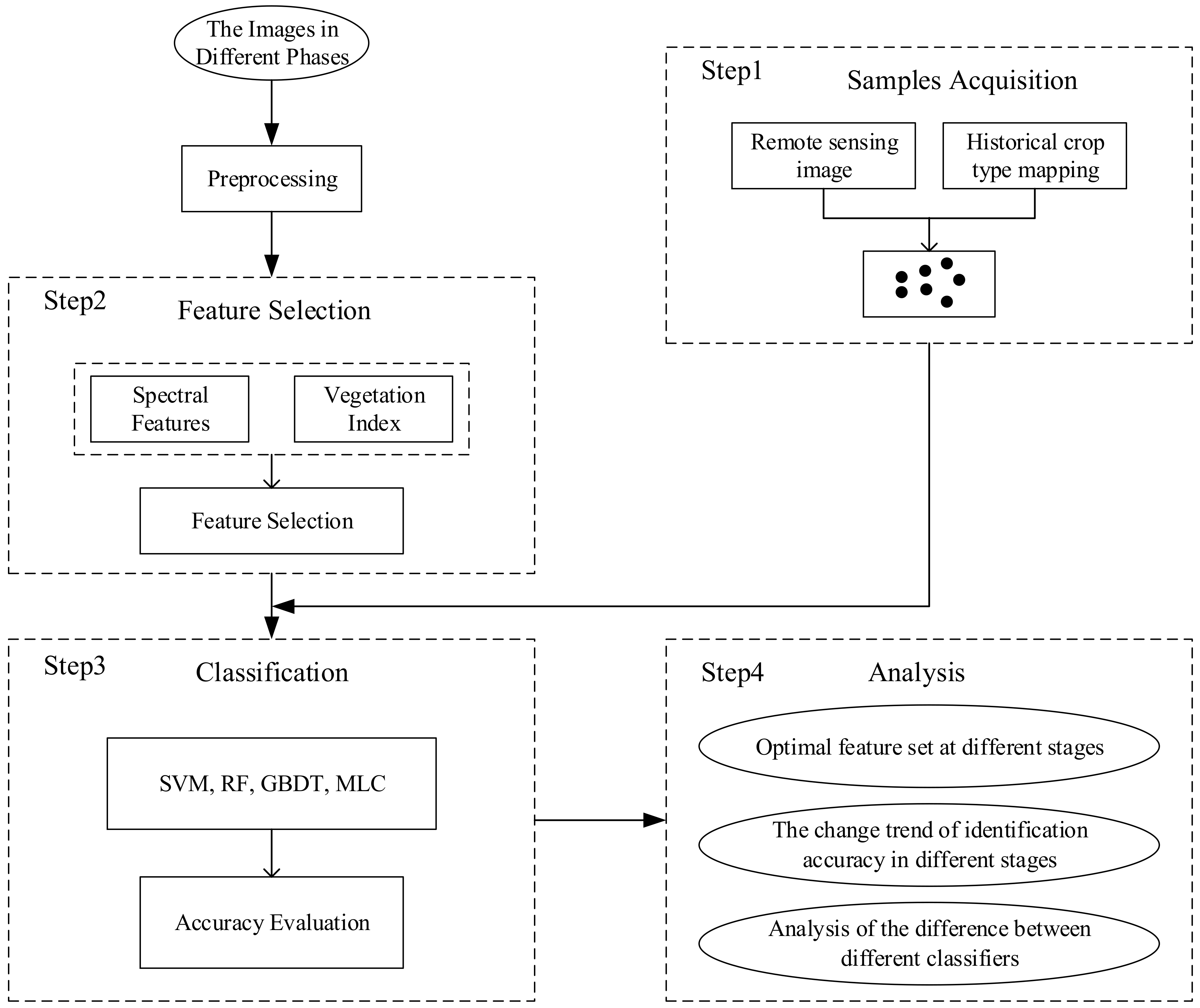
The historical crop maps from 2019 of Heilongjiang Province were also collected, which could help effectively construct training sample generation work by combining remote sensing images from 2020, to simplify the workload of manual labeled samples and ensure the progress of the following research contents. The data came from the research results of Zhao et al. [32]. A binary indicator featuring high separability for single crop (corn, rice, and soybeans) based on Sentinel-2 images was proposed by them, and then they used the image adaptive threshold segmentation method to obtain crop-type mapping in Heilongjiang Province based on the binary indicative features of the three crops. With this method, the crop-type mapping was identified with an overall accuracy of 93.12% and kappa coefficient of 0.90. A detailed review of this paper and accuracy information can be found in the article [32].

3. Method

At present, there are three problems that exist in early crop recognition: (i) The problem that the ground samples are difficult to obtain in real time. (ii) Which features are most important at different stages. (iii) What precision level can crops achieve at different stages, and the differences in early identification of crops among different classifiers, still lack a systematic summary. To solve the above problems, three parts were designed to study the early identification of crops in Northeast China. First, acquiring the training samples automatically, historical crop maps from 2019 and remote sensing images from 2020 were used to generate samples, which solved the problem that samples were difficult to obtain in real time. Second, selecting the optimal features, the Mean Decrease Accuracy (MDA) feature selection method was used to calculate feature importance. Therefore, the optimal feature set at different stages could be obtained. Third, identifying the crops with different classifiers and using the field samples for accuracy verification. Finally, the characteristic of crop accuracy levels in the different stages, the earliest identifiable time of each crop, as well as the difference among different classifiers were analyzed. The overall technical illustration is shown in Figure 3.

3.1. Automatic Sample Construction Based on Historical Crop Maps

Studies have shown that major crops vary little in neighboring years [7,20,30]. Based on the foundation, a method to automatically obtain current year samples based on historical crop type mapping was designed. First, the crop type mapping from 2019 was used to segment the remote sensing images from 2020, so that the candidate area image of each category could be obtained. Then, K-means clustering was used to obtain the clustering results in each candidate area image, and an appropriate threshold was set to obtain the pure sample area of each candidate area. Finally, training samples were randomly generated in the pure sample area (Figure 4). All the samples acquired based on the above method were used as training samples. The whole processing chain for automatic sample construction is summarized in the following sections.
First, the acquisition of candidate region image. Three remote sensing images with good visual separability from 2020 were used in our three study areas (August 22, August 21 and August 23), and they were segmented with historical crop maps from 2019, so that the 2020 corn candidate area, rice candidate area, soybeans candidate area, and other candidate areas of each study area could be obtained.
Second, the unsupervised clustering of images. K-means is a popular unsupervised clustering algorithm, which has the advantages of simple principle, fast processing, and good effect [6]. Euclidean Distance (ED) is commonly used as an indicator to measure the similarity between data objects when using the K-means algorithm to classify remote sensing images, and the similarity is inversely proportional to the distance between data objects; that is, the smaller the distance between objects, the greater the similarity [33]. The main principle of obtaining the classification results of candidate region by K-means clustering method is: (1) In order to make the unsupervised clustering results more detailed, 12 initial points were selected as centroids for each candidate region image, and the pixels were classified into the most similar class by calculating the similarity between each pixel and the centroid; (2) The centroid of each class was recalculated, and this process was repeated until the centroid did not change, and which class each pixel belonged to was determined. Finally, the 12 sub-cluster results were obtained in each candidate areas.
Third, the determination of pure crop planting area. Its determination needed to be based on the classification results of the previous step. Specifically, the 12 sub-cluster results of each candidate region were ranked by area from the largest to smallest, and clusters ranked in the top 40% were selected as the candidate region category. The threshold was set at 40%, mainly considering that the principle of the sample could be missed, but that the error could not be allowed. If the threshold value is set too high, the target sample range increases, but other ground objects will be introduced, leading to an impure sample; if the threshold value is set too low, the target sample will not be representative. Therefore, 40% is a good trade-off, avoiding the introduction of other crop samples while maintaining the significant representativeness of samples.
Finally, the construction of sample set. The pure sample area was converted to vector data, and the vectorization results were composed of many sub-vector areas, then the area of these sub-vector regions was calculated and training sample points of the ground object in the top N sub-vector regions with the largest area were randomly generated (N represents the number of training samples of the ground object). Some ground features, such as buildings, woodlands, and rivers, were unified as an “other” class in the historical crop maps, which was not suitable for the method we proposed. Therefore, the acquisition of these samples needed to be combined with relevant interpretation knowledge to manually label the samples of these ground objects. All the training samples in the three regions are shown in Table 3.
All generated training samples in the three study areas were used for training our classification model, and its effectiveness was verified from two parts:
(1) Jeffries–Matusita (J-M) distance was used to evaluate the sample separability between each two ground objects [34]; The J value ranges from 0 to 2. In general, the larger the value, the better the separability. When the value is less than 1, it is considered that the two types of samples are not separable. When the value is less than 1.8, it indicates that the sample features is moderately separable. However, when the value exceeds 1.9, it indicates that the sample features have good separability. Its formula is as follows:
J = 2 1 e B
J is the value of J-M distance, and B is the Bavarian distance between the two sample categories. Its calculation formula is
B = 1 8 m 1 m 2 2 2 δ 1 2 + δ 2 2 + 1 2 ln δ 1 2 + δ 2 2 2 δ 1 δ 2
m 1 and m 2 represent the mean values of the spectral reflectance of classes 1 and 2, respectively. δ 1 and δ 2 represent the standard deviation of the spectral reflectance of classes 1 and 2, respectively.
(2) Random Forest (RF) has the advantage of fast training speed and relatively simple implementation. Therefore, we used these samples tried to perform a preliminary classification of RF, and then evaluated the quality of the samples based on the classification results.

3.2. Feature Preparation

To improve the identification ability of crops, 10 original bands, including B2, B3, B4, B5, B6, B7, B8, B8A, B11, and B12, and 16 most commonly used vegetation indices related to crop identification, were used (Table 4) in our study. The bands of B1, B9, and B10 were eliminated due to their coarser spatial resolution (60 m).

3.3. Crop Classification Model

In our study, Support Vector Machine (SVM), RF, Gradient Boosting Decision Tree (GBDT) and Maximum Likelihood Classification (MLC) were used to compare their differences in early-stage crop recognition. These four methods were selected on the basis of their wide application and reliability in land cover classifications. The parameter settings of different classifiers are shown in Table 5.
SVM has significant advantages in small samples, nonlinear problems, and high-dimensional data processing [50,51,52]. Usually, the SVM algorithm solves binary classification (two-dimensional) problems through finding the separation hyperplane that can divide the training dataset correctly and the geometric interval maximally; however, for multi-classifications, it is more complex. Specifically, in the n-dimensional space, an optimal segmentation surface (kernel function) is used to map it to the high-dimensional space to maximize the separation of the two types of samples, thus making multi-classification linear solvable. Finally, multi-classification is realized through combining multiple binary classifiers [53,54,55]. Radial Basis Function (RBF) is usually chosen as the kernel function when using SVM to classify remote sensing images, because it provides a trade-off between time efficiency and accuracy. There are two parameters in the RBF kernel that need to be optimized: the penalty coefficient (cost) and gamma, cost controls the complexity and generality of the model, and gamma determines the extent and width of the input space. Generally, a larger cost value will not only lead to overfitting but also increase the calculation time, and inappropriate gamma values will lead to inadequate model accuracy or introduce errors. After many experiments, a better accuracy can be achieved when the value of cost was set to 50 and the value of gamma was set to 0.8.
RF has been widely used due to its high speed, high accuracy, and good stability [56,57,58,59,60]. Which is an ensemble machine learning technique that combines multiple trees. Each tree uses the bootstrap sampling strategy to create about 2/3 of the training samples from the original dataset and generates a decision tree for each training samples separately, and the remaining about 1/3 of the training samples are used as Out-of-Bag (OOB) data for internal cross-checking. Finally, the final classification results are determined by voting according to the classification results of all trees. There are two key parameters in RF that need to be optimized: the number of randomly selected features used to segment each node (mtry), and the number of trees (ntree). To balance the accuracy and calculation time, ntree was set to 100 in our study. In general, mtry is set to the square root of ntree, which was 10.
GBDT is an iterative decision tree algorithm, which is composed of multiple decision trees, and the conclusions of all trees are accumulated to obtain the final result. Unlike RF, this algorithm builds a weak learner at each step of the iteration to compensate for the shortcomings of the original model. Therefore, it has the characteristics of strong generalization ability and high classification accuracy [61,62]. Its key parameters are: the number of decision trees to be created (numberOfTree), the learning rate (shrinkage), and the max depth of tree (maxDepth), the sampling rate for stochastic tree boosting (samplingRate), all of these optimized parameters can help improve the performance of the model in terms of speed and accuracy.
MLC is one of the most well-known and widely used classification algorithms in remote sensing, which has the advantage of being a simple principle and easy to implement [63,64,65,66,67]. It assumes that each type of statistic in each band is normally distributed, and then the likelihood that a given pixel belongs to a certain training sample is calculated, and finally the pixel merges into the class with the highest likelihood. However, this classification method is not encapsulated in GEE; the method was conducted in Environment for Visualizing Images (ENVI) software. The setting of the data scale factor parameter adopted default value 1.0.

3.4. Feature Optimization

The MDA feature optimization method was used to evaluate the importance of features at each stage. The MDA feature ranking method uses OOB error to evaluate the variable importance (VI) [68,69]. Its principle to evaluate the importance of features is that if random noise is added to the feature, the accuracy of OOB data classification will be greatly reduced, which indicates that this feature has a great impact on sample prediction, which in turn indicates that the feature has higher importance. The calculation formula of VI is as follows:
V I M A = 1 N t = 1 N B n t M A B O t M A
where VI represents the importance of different features, M A represents a feature, N is the number of decision trees, B n t M A represents the OOB error of the t-th decision tree when M A is not added, and B O t M A is the OOB error of the t-th decision tree when M A is added with noise interference.
A previous study proved that there was no increase in crop identification accuracy when the number of features used exceeded 15 [70]. In order to trade-off between accuracy and computational cost, the top 15 features with the largest values were selected as the optimal features, and used for image classification.

3.5. Accuracy Assessment

In this study, overall accuracy (OA), kappa, producer accuracy (PA), user accuracy (UA), and F score were calculated according to the confusion matrix to evaluate the accuracy of the classification results.
The OA and kappa values represent the accuracy assessment of the global performance of our classification results [70]. Specifically, the OA represents the proportion of all samples that were correctly classified. kappa is a measure range 0–1 and quantifies the model prediction results and the actual classification results, while the PA, UA, and F score values represent the accuracy assessment of individual crop type [71]. PA represents the proportion of the correct classification results of a certain class to its validation samples, and it reflects the omission. UA represents the proportion of the correct classification results of a certain class to the user’s own classification results, and it reflects the misclassification. In general, PA and UA have contradictory relations, and they cannot achieve high classification accuracy at the same time. F score is a comprehensive indicator composed of PA and UA, which can comprehensively evaluate the performance of the classifier in single crop [72]. Studies have shown that the 85% crop recognition accuracy can basically meet the agricultural applications of crop type mapping [73]. Therefore, the earliest identification time of each crop was defined as the first time when the F score value was greater than 85% in this paper. The formula of F score is:
F score = 2 × PA UA PA + UA 100 %

4. Results and Discussion

4.1. Automatic Sample Construction and Analysis of Sample Separability

The distributions of training sample points, generated based on the historical crop maps and remote sensing images in our three study areas, are shown in Figure 5, and the classification results and accuracy of RF based on these samples are shown in Figure 6 and Figure 7, respectively.
The J-M distance was used to measure the degree of separability between each pair-wise crop, and all the J-M values in our study area were above 1.9, indicating these samples have good separability, and the OA and kappa coefficient of RF in the three study areas all reached about 99%. The above two results showed that the automatic generation method of sample points could be realized based on historical crop maps and remote sensing images, and the generated samples could be used for image classification work at different periods of the three study areas.

4.2. The Optimal Features and Changes in Different Stages

In this study, the MDA feature optimization method was used to obtain the optimal features of the different periods in our three study areas (Table A1, Table A2 and Table A3). To analyze which features were important in the early stages (April–June), middle stages (July–August), and late stages (September–early October), the common top rankings feature of the different periods in each growth stage in our three study areas were summarized (Table 6).
At the early stage of crop growth (April–June), rice was basically covered with water; it was a mixture of water and rice in the image, while corn and soybeans were in a state of the sowing and emergence period. The height of the crops was low, and had low green vegetation and soil background in the image. Among the spectral characteristics, B12 was the most prominent, mainly because the short-wave infrared band was more sensitive to water information. The LSWI, which was composed of the short-wave infrared band, also contributed relatively high in this stage. In addition, traces of wheat stubble harvested from the previous season existed, and many farmlands were in a state of bare tillage. Therefore, the NDSVI and NDTI also played a key role in crop identification during this stage.
At the middle stage of crop growth (July–August), all crops in the study area gradually entered vigorous growth, and the vegetation coverage gradually reached the maximum. Due to the relatively high vegetation coverage and chlorophyll water content, the advantage of the red-edge vegetation index was also reflected. In general, the important features were B12, B11, B8, LSWI, NRED2, RENDVI, and so on, which, according to these features, could better identify crops at this stage.
At the late stage of crop growth (September–early October) into the late stage of the crop, the leaves gradually turned yellow and dried until harvest. In general, NDTI, B11, NDSVI, and other indicators made full use of the short-wave infrared band to represent the water and vegetation residual coverage. Therefore, they made a relatively large contribution to the identification of crops in this stage.

4.3. Variation Characteristics of Crop Identification Accuracy at Different Stages

In this study, the optimal feature sets for different periods (Table A1, Table A2 and Table A3) were used as the input of four classifiers (SVM, GBDT, RF, and MLC) to identify crops. The crop recognition accuracy in different periods could be obtained (Figure 8, Figure 9 and Figure 10). Figure 8 and Figure 9 show that the accuracy trends of corn and soybeans in the three study areas were similar, which increased slowly in the initial stage and then entered a rapid increase period, after which, it gradually tended to be in a stable state after reaching the maximum value. However, the change in amplitude of rice identification accuracy was relatively smaller because of its higher initial value; after reaching the maximum value, it was in a state of fluctuating up and down (Figure 10). To analyze what accuracy each crop can achieve at different stages, the lowest and highest values for all periods at each stage in our three study areas were taken as the accuracy level of this stage.

4.3.1. The Recognition Accuracy Level of Corn at Different Stages

Figure 8 shows that the identification levels of corn at different phases, and its recognition accuracy level were analyzed as follows:
At the early stage of crop growth (April–June), the identification accuracy of soybeans was between 40% and 79%. Its accuracy was low and could not meet the basic requirements of corn identification. With the addition of images, the recognition accuracy of GBDT was higher than that of other classifiers in Region 1 and Region 2, and it could achieve the highest accuracy of 79% with four images in Region 2 among the three study areas. In Region 3, RF performed better than that of other classifiers with 2~4 images, and SVM was slightly lower than RF. However, MLC performed poorly compared to other classifiers in the three study areas.
At the middle stage of crop growth (July–August), the identification accuracy of corn in the three study areas was between 79% and 100% during this stage. The accuracy in this stage basically reached the maximum value, which could meet the demand of crop mapping. In Region 2 and Region 3, the recognition accuracy of corn with four classifiers using five images was all greater than 86% on July 2. However, the earliest recognition time of corn in Region 1 was a little later than that of the other two study areas; its recognition accuracy of four classifiers with seven images was all greater than 93% as early as July 13. These results indicated that the high-precision identification of corn could be identified in early July at the earliest identification time, and the identification accuracy was above 86%. At this stage, GBDT performed better than other classifiers, SVM and RF performed after GBDT, and MLC performed worse in the three study areas.
At the late stage of crop growth (September–early October), corn was basically harvested. Its accuracy ranged between 90% and 100%, and basically remained in a stable state during this stage. The performance of the classifier in this stage was similar to that of the previous stage. The recognition accuracy of GBDT, RF, and SVM was comparable and higher than that of MLC.

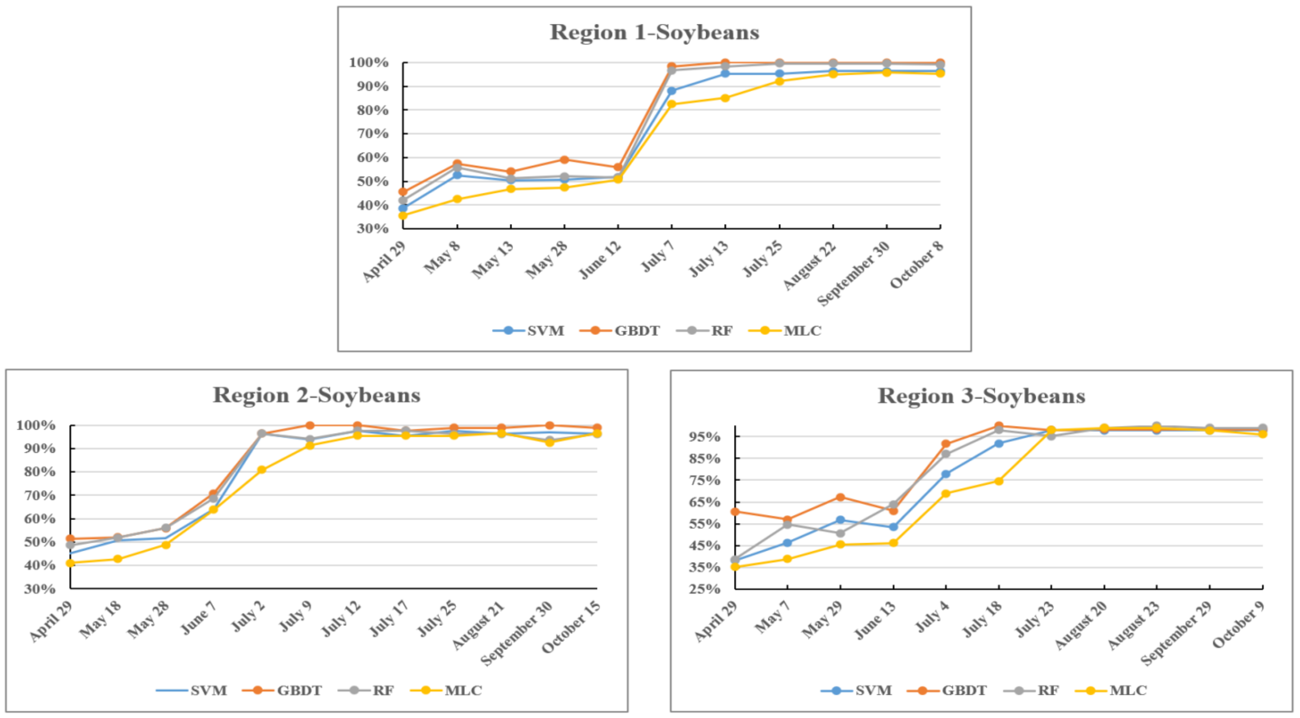
4.3.2. The Recognition Accuracy Level of Soybeans at Different Stages

It can be seen from Figure 9, the identification levels of soybeans at different stages were analyzed as follows:
At the early stage of crop growth (April–June), the identification accuracy of soybeans was between 35% and 71%, which was lower and could not meet the basic requirements of soybeans mapping in this stage. Among all the classifiers, the accuracy of GBDT was higher than other classifiers in the three study areas, and it could achieve the highest recognition accuracy of 71% with four images in Region 2 among the three study areas. RF and SVM performed comparably in Region 1 and Region 2, and MLC performed worse than other classifiers in the three study areas.
At the middle stage of crop growth (July–August), the accuracy of soybeans in the three study areas ranged between 69% and 100%, With the addition of more images, the accuracy in this stage gradually reached saturation, and the identification accuracy of soybeans in many periods could achieve satisfactory accuracy during this stage. In Region 2, the recognition accuracy of soybeans with GBDT, RF, and SVM reached 96% with five images on July 2. In Region 3, the recognition accuracy of soybeans with GBDT and RF was 91% and 87% with five images on July 4, respectively. In Region 1, the recognition accuracy of soybeans with SVM, GBDT, and RF was all higher than 91% with six images on July 7. However, MLC needed to use six images to reach the earliest high-precision identification accuracy of 93% on July 9 (Region 2). These results showed that the early high-precision identification of soybeans could be obtained in early July, and the identification accuracy was as high as 87%.
At the late stage of crop growth (September–early October), soybeans were basically harvested. Its identification accuracy ranged between 92% and 100%. The recognition accuracy of the four classifiers was basically in a saturated state compared with the previous several stages, and the accuracy did not increase very much with more images added.

4.3.3. The Recognition Accuracy Level of Rice at Different Stages

It can be seen from Figure 10, the identification levels of rice at different stages were analyzed as follows:
At the early stage of crop growth (April–May), the recognition accuracy of rice ranged between 58% and 100%. In Region 2 and Region 3, the recognition accuracy of GBDT and RF could achieve 86% with one image as early as April 29. However, in Region 1, SVM, GBDT, and RF could use four images to realize early identification of rice as early as May 28 with an identification accuracy up to 88%. These results showed that the early high-precision identification of rice could be obtained as early as the end of April. Among all the classifiers, the initial recognition accuracy of GBDT was much higher than that of other classifiers, followed by RF and SVM, and MLC was lower than other classifiers in the three study areas.
In the middle stage of crop growth (July–August), the recognition accuracy of rice ranged between 93% and 100% during this stage. In the late stage of crop growth (September–early October), the rice was basically harvested in early October. Its recognition accuracy ranged between 96% and 100% during this stage. In Region 2 and Region 3, the accuracy fluctuated upwards and downwards with more images added, GBDT and RF performed comparably in the three study areas, followed by SVM, and MLC performed lower than other classifiers in the three study areas.
In general, the identification accuracy of the three crops in the early stage of crop growth was less than that in the middle stage, and the accuracy in the late stage was the best and basically in a stable state. Corn and soybeans had similar phenological periods, and the accuracies of the two crops were similar. The early identification of the two crops could be realized in early July at the earliest identification time; they were in the seven leaves period and the blooming period, respectively. The early identification of rice could be realized at the end of April at the earliest identification time (the flooding period) due to its characteristics being different to those of the former two crops. In terms of the whole process of crop recognition, GBDT and RF performed better than SVM and MLC.

4.4. Potential Analysis of Early Crop Identification

Timely and accurately acquisition of early crop information has important scientific significance and practical value. It can not only provide basic information for agriculture-related decisions and applications, but also can be used to support national food security, market planning, and many other social economic activities. This study systematically evaluated the potential of early crop identification in Northeast China based on Sentinel-2 image data, and the recognition abilities of the three crops in different growth stages are presented below.
In the early stage of crop growth (April–June), the recognition accuracies of corn, soybeans and rice were 40~79%, 35~71%, and 58~99%, respectively. Corn and soybeans appeared as bare land, and their accuracies were low and could not meet the requirements of early recognition accuracy in this stage. Rice was basically covered by water in this stage, which was a mixture of water and rice in the image, and the short-wave infrared band was more sensitive to the water content information [74]. Therefore, B12, LSWI, and NDTI ranked relatively higher in the optimal feature set and played an important role in crop identification in this stage [75]. Combined with GBDT and RF classifiers, the earliest high-precision recognition date of rice occurred on April 29, and the accuracy was as high as 86%. Therefore, we made a conclusion that rice could be identified as early as the end of April (the flooding period). This conclusion was consistent with the early identification time of rice obtained in the literature [76,77]. In the middle stage of crop growth (July–August), the recognition accuracies of corn and soybeans were 79~100% and 69~100%, respectively. Corn and soybeans gradually entered a vigorous growth stage. During this stage, the cover density and the chlorophyll water content of soybeans were higher than those of corn [78]. Short-wave infrared bands, NRED2 and red-edge index of vegetation, played an important role in crop identification in this stage. Combining the four classifiers could identify corn and soybeans as early as July 2, and their recognition accuracy was as high as 86% and 87%, respectively. Therefore, we concluded that the earliest identifiable times of corn and soybeans occurred in early July, and the phenological stages were in the seven-leaf period and flowering period, respectively. It has been mentioned in articles [72,79] that corn could be identified at the earliest period of seven leaves and soybeans at the earliest period of flowering. Moreover, some other findings were found when analyzing the experimental results, which are discussed below: from the recognition accuracy of corn in the whole period of the three regions, it can be found that the early stage was more susceptible to the influence of the crop planting structure, while the middle and later stages were less affected. Taking the recognition accuracy of corn in the early stage as an example, the identification accuracy of corn in Region 2 was higher than that in Region 3, and the Region3 than that in Region1 during this stage. There were also some differences in the earliest identified time of the three regions, and corn was the earliest identified crop in early July in Regions 2 and 3, while in Region 1, it was slightly later, which was in mid-July. Therefore, the early identification of crops was closely related to the planting structure of crops; that is, the planting structure was relatively simple, the farmlands were relatively regular, and the accuracy of crop identification was higher [80]. In contrast, the more complex the planting structure was, the lower the crop identification accuracy [81,82], thus delaying the time of early crop identification.
From crop emergence to harvest, with the addition of images, crop recognition accuracy gradually increases in the early stages, while in the middle and late stages, it gradually becomes stable. As mentioned above, in the early stage, the rice information is more prominent in this stage due to its own characteristics, while the information of corn and soybeans are weak, and the rice information can be enhanced by some key features, while the information of corn and soybeans is more difficult to capture. Therefore, the recognition accuracy of rice was higher than that of corn and soybeans in this stage. In the middle stage, the uniqueness of corn and soybeans gradually emerges, and these two crops’ information can be well captured by some key separable features, and the addition of these features greatly improves the accuracy of crops. In the late stage, the crops enter a mature and harvest period, and the accuracy was in a saturated state. Due to the incremental design method used for the image data, some previous key features also played an important role on these periods in the late stage, so the accuracy in this stage was also high. Previous studies have shown that a high classification accuracy can be achieved by using the images in only a few optimal dates. However, the accuracy may change to a saturated or decreased state as more images are added [3,20,83], and our results were consistent with these conclusions.
The problem that early crop identification cannot be carried out due to a lack of samples. Considering that the historical crop map has a large amount of prior knowledge, if the knowledge was fully utilized, it will help to solve the sample problem. Therefore, we proposed an automatic sample generation method to generate training samples based on the historical crop map and remote sensing images, which solved the difficulty of obtaining samples in real time, and this also can be applied to other regions with little difference in crop planting structure from year to year. Then, the feature optimization method was used to calculate the feature importance in different periods; from which we summarized the key recognition feature in different stages to provide a reference for relevant crop recognition research in selecting effective recognition features and reducing the blindness in feature selection. Finally, four commonly used classifiers were used to identify crops in different periods. From which we summarized the accuracy variation characteristics of crops at different stages and the earliest identifiable date that each crop can reach. In addition, the difference in the performance of the classifiers was also analyzed, and it was found that GBDT and RF were better than SVM and MLC in terms of the recognition of crops at different stages. Although GBDT was not as popular as the other three classifiers, it showed better accuracy in our three study areas, and can provide a new reference for the selection of classifiers for crop identification research.
Limited by the resolution of Sentinel-2 images, the spectral and vegetation index features were only considered in our study, but texture features also contribute significantly to crop identification. Next, satellite data with higher spatial resolution will be considered to comprehensively evaluate the performance of spectral, vegetation index, and texture features in different periods. Additionally, Deep Learning (DL) technology is more and more prominent in the field of remote sensing classification [84,85,86]. Therefore, research on the comparison between DL algorithms and traditional classifiers in terms of classification effect and model transfer ability is also the direction of future efforts.

5. Conclusions

In this study, three important contents of early crop identification at three sites in Heilongjiang Province were explored. First, the method of sample points generation based on historical crop maps solved the problem that the ground samples could not be obtained in real time in the early crop stage. Then, MDA was used to optimize the optimal feature sets at different phases. Finally, four classifiers were used to identify crops, and the variation characteristics of crop recognition accuracy at different phases and the differences among different classifiers were analyzed from this part. The main conclusions are below.
(1)
The identification accuracy of corn in the early growth stage was between 40% and 79%, while in the middle stage, it could reach 79~100%, and in the late stage, it was between 90% and 100%. The earliest identification time of corn could be obtained in early July (the seven leaves stage), and the identification accuracy was up to 86%. The identification accuracy of soybeans in the early growth stage was between 35% and 71%, while in the middle stage, it could reach 69~100%, and in the later stage, it was between 92% and 100%. The earliest identification time of soybeans could also be obtained in early July (the blooming stage), and the identification accuracy was up to 87%. The identification accuracy of rice in the early growth stage was between 58% and 100%, while in the middle stage, it could reach 93~100%, and in the late stage, it was between 96% and 100%. The earliest identification time of rice could be obtained at the end of April (the flooding period), and the identification accuracy was up to 86%.
(2)
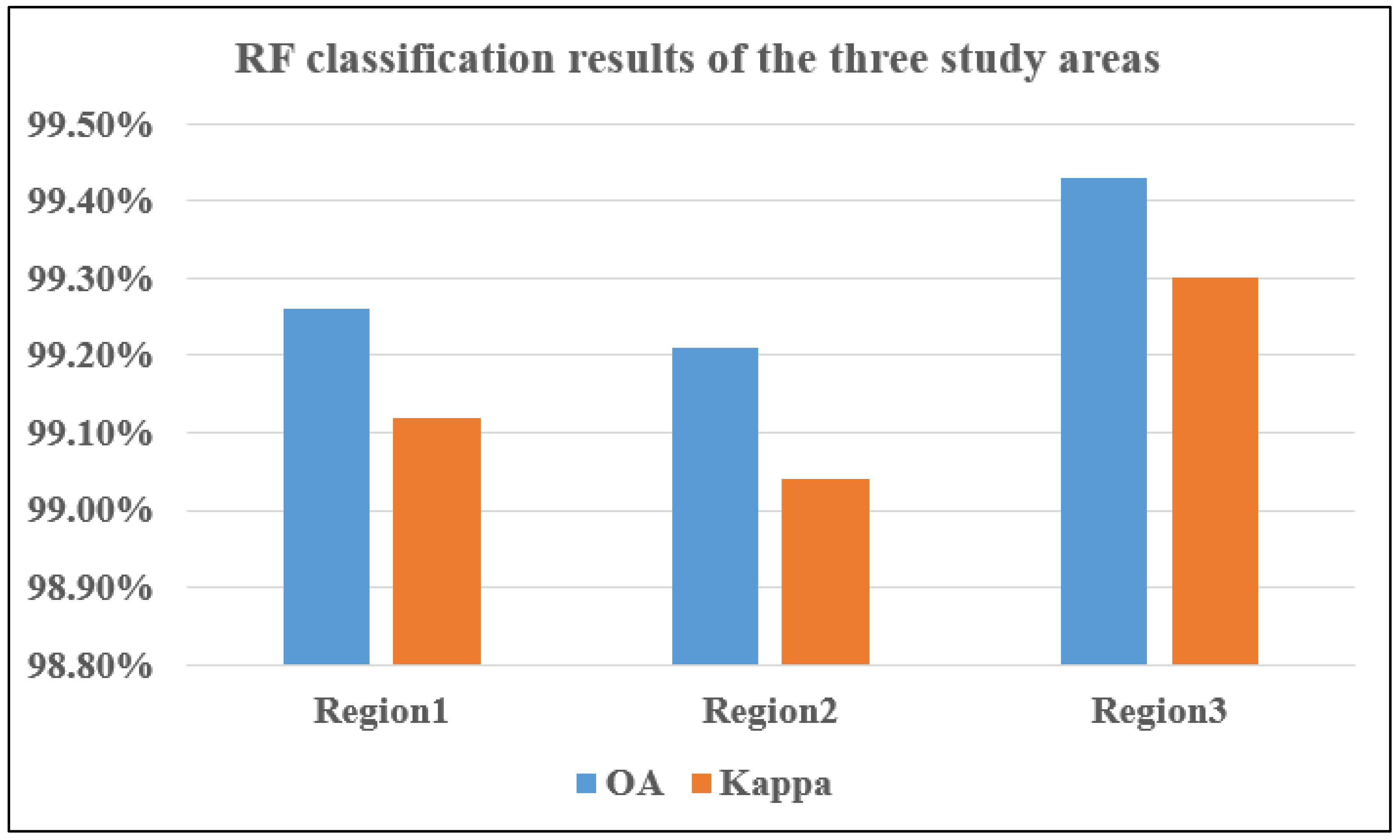
GBDT and RF performed better in the whole growth phases and had higher recognition accuracy than other classifiers. Therefore, they are recommended crop early recognition research.
(3)
In the early stage, B12, NDTI, LSWI, and NDSVI played important roles in identifying the crops. In the middle stage, features such as B12, B11, B8, LSWI, NRED2, and RENDVI contributed greatly. In the late stage, NDTI, B11, and NDSVI were important in identifying the crops.
(4)
It was effective in acquiring training samples based on crop-type mapping and remote sensing data, which could effectively reduce the workload of manual sample selection, and it is of great significance for large area and real-time crop mapping.

Author Contributions

Conceptualization, M.W. and Q.L.; methodology, M.W., H.W. and Y.Z.; software, M.W.; validation, M.W. and H.W.; formal analysis, M.W.; investigation, M.W., H.W., G.S. and Y.R.; writing—original draft preparation, M.W. and H.W.; writing—review and editing, M.W.; visualization, M.W.; funding acquisition, Q.L. and X.D. All authors have read and agreed to the published version of the manuscript.

Funding

This research was funded by the National Key R&D Program of China (Grant No. 2021YFD1500103), the National Science Foundation of China (Grant No. 42071403), and the Key Program of High-resolution Earth Observation System (Grant No. 11-Y20A16–9001-17/18-4).

Conflicts of Interest

The authors declare no conflict of interest.

Appendix A

Table A1. Optimal feature sets at different periods in Region1.
PhaseApril 29May 8May 13May 28June 12July 7July 13July 25August 22September 30October 8
Rank
by
feature
importance
B12NDTINDTILSWI_3B12_4B5_5B12_6B8_7NRED2_8B12_4NDTI_8
NDTILSWIOSAVI_2NDSVI_3NRED2_3B12_5LSWI_4B11_4B12_4B12_7B5_7
B7RENDVI_1LSWINDTIB2_4RENDVI_5B5_6B12_4NDTI_7B11_4NDSVI_8
NDSVINRED2_1B2NRED2_3NRED1_3B8_5B11_6B3_6B5_8NRED3_8B12_6
RENDVINDVI_1NDSVI_1B12_3WDRVI_3NRED3_5B12_4B2_6B11_7B5_7B12_5
LSWINRED2LSWI_2WDRVI_1LSWI_3B12_4NDSVI_5NDTI_7B11_4RENDVI_7B8A_8
NRED1WDRVI_1NDSVI_2NRED1_3NDVI_3NDVI_5B2_4B12_6B8A_8B11_7B11_7
B11NDSVINDVI_1EVI_3B4_2B11_4B11_4NDTI_4NRED2_8B11_8B12_3
WDRVIB11B4_2B11_2TVI_2RENDVI_5NDSVI_6B12_7B5_8B3_8B11_9
TVINRED1_1B2_2GNDVI_2VIgreen_4LSWI_5B4_6NDVI_7LSWI_6B3_6B11_4
EVITVI_1WDRVI_2B11_3WDRVI_1EVI_5B11_3B11_7B11_6EVI_3B11_8
NDVIMCARI_1NDVI_2NDVI_3B2_2VIgreen_5NDVI_6B3_7LSWI_4NDSVI_4MCARI_10
MCARINDTI_1TVI_1MCARI_3B4_4NDSVI_5B4_5NDSVI_6NDSVI_4B12_5B4_6
B4NRED3_1B11GCVI_3NDSVI_4B3_5LSWI_6NRED2_6B12_6B12_3LSWI_9
B5GNDVI_1RENDVI_1NDTI_2B11_4OSAVI_2B2_6NDSVI_4B3_6OSAVI_7RENDVI_8
Table A2. Optimal feature sets at different periods in Region 2.
PhaseApril 29May 18May 28June 7July 2July 9July 12July 17July 25August 21September 30October 15
Rank
by feature importance
TVINDSVI_1LSWILSWI_3B11_4B11_5B12_6B12_6B8_6B11_9B12_6NDTI_2
LSWINDSVIB11_1B11_2B11_4NDSVI_4B12_5NDSVI_2LSWI_8B11_7B11_7B12_8
NDTIB2_1B12_1B12_2EVI_4NRED2_5RENDVI_6B11_7B11_2B11_3NDSVI_2B11_8
RENDVILSWI_1GNDVINDSVI_2B2_4B12_5B2_5B11_2B5_7NDSVI_6B11_3RENDVI_5
NDSVITVIB2_1NDSVI_3B12_4B5_4B11_5B4_7B12_5B11_9B12_7NRED2_6
B11B6_1OSAVI_1B12_2NRED1_4B2_2B5_5NDSVI_5NDSVI_7B4_2NRED3_8B12_2
VIgreenGNDVI_1GCVI_1DVI_2OSAVI_4B12_5B11_5NRED2_7B12_2NRED3_6NRED1_2GCVI_8
EVIB12_1RENDVI_1NRED2B12_4B4_5NDSVI_5LSWI_2B3_3LSWI_2B3_3B12_9
B12NRED2_1NRED1_1TVI_1NDSVI_3LSWI_3LSWI_3NRED3_4NDSVI_4LSWI_3LSWI_3B11_2
WDRVINDSVI_1TVINRED1_2NRED2_3B11_2B3_2B12_2B12_6NDSVI_6DVI_5NDSVI_3
NRED2NRED3_1NDSVI_2NDTI_3NDTI_4NDSVI_2WDRVI_7B12_7B11_2B12_2RVI_7NRED3_7
B4NRED1_1WDRVIB3_3RVI_4NRED2_4NDSVI_2LSWI_4NRED3_2NDSVI_1NDTI_2NDSVI_3
B2B4_1NDTIWDRVI_3LSWI_2RVI_4B5_6VIgreen_5EVI_7B12_8B12_4B2_8
B8AB6_1B12_2B5_3TVI_4NDVI_2B12_2NDSVI_6NDTI_2NDTI_2MCARI_8B8A_2
B3NRED2B2_2B8A_3B11_3DVI_5NRED3_6B5_2B11_6NRED2_8LSWI_7DVI_8
Table A3. Optimal feature sets at different periods in Region 3.
PhaseApril 29May 7May 29June 13July 4July 18July 23August 20August 23September 29October 9
Rank
by
feature importance
NDTINDTIB12_2NDSVI_3GNDVI_4B3_5NDSVI_6LSWI_7RENDVI_8NDSVI_3NDSVI_3
TVINDTI_1OSAVI_2NRED2_3B12_4B11_5NRED2_6B5_7B8_2B6_7NDTI_7
LSWINDSVI_1NDTI_2B11_3B11_4B11_5B12_6NDTI_7B11_7B11_6EVI_2
B12LSWI_1NDTI_2RVI_2WDRVI_4NRED2_4B5_2NDSVI_7NDWI_8NRED3_5NDSVI_8
NDSVIRENDVILSWI_2NDWI_2NDSVI_2B12_2NDTI_6NDSVI_3NRED2_2NDVI_7NDTI_8
RENDVITVI_1NDSVIDVI_2NRED2_2B11_5B11_1B11_7B11_7OSAVI_8B6_8
B5WDRVITVI_2NRED1_1NRED1_2B5_5B11_6B12_7B12_8B5_6MCARI_8
NRED1B11_1B11B2B3_4B5_5B11_4NRED1_7B12_7NDSVI_2WDRVI_8
NRED2B3_1NDTI_1NRED2_2NDSVI_1VIgreen_5B3_5B11_5B3_7NRED1_7B3_1
B11NRED1VIgreen_2MCARIVIgreen_2NDSVI_5B3_6B12_7B11_8B11_3OSAVI_8
VIgreenTVIEVI_2OSAVI_3NDWI_4NDSVI_5NDSVI_4EVI_6B12_8NRED2_5NRED3_8
NDVINDVINRED2B12_2NRED3_4B12_5B4_6B5_7B8_6EVI_2B12_8
EVINDVI_1NRED1_1NRED1_2RENDVI_3EVI_5B2_6RVI_7B12_6B7_7NDSVI_5
NRED3RVIRVI_2NRED1_1EVI_4RENDVI_5B2_6RENDVI_6NDSVI_2B12_7B11_7
GNDVIRENDVINDTI_1B12B11_2B12_5NRED1_6RENDVI_6TVI_3NRED3_8B8A_7
Note: This study uses an incremental image data design. The features of the first period have no suffix, and the suffixes of the features of each subsequent period are incremented by 1. For example, _1 represents the features used in the second period of each region, _2 represents the features used in the third period in each region.

References

  1. Valero, S.; Arnaud, L.; Planells, M.; Ceschia, E. Synergy of Sentinel-1 and Sentinel-2 Imagery for Early Seasonal Agricultural Crop Mapping. Remote Sens. 2021, 13, 4891. [Google Scholar] [CrossRef]
  2. Demarez, V.; Helen, F.; Marais-Sicre, C.; Baup, F. In-Season Mapping of Irrigated Crops Using Landsat 8 and Sentinel-1 Time Series. Remote Sens. 2019, 11, 118. [Google Scholar] [CrossRef] [Green Version]
  3. Hao, P.Y.; Zhan, Y.L.; Wang, L.; Niu, Z.; Shakir, M. Feature Selection of Time Series MODIS Data for Early Crop Classification Using Random Forest: A Case Study in Kansas, USA. Remote Sens. 2015, 7, 5347–5369. [Google Scholar] [CrossRef] [Green Version]
  4. Chen, Z.; Ren, J.; Tang, H.; Shi, Y.; Liu, J. Progress and perspectives on agricultural remote sensing research and applications in China. J. Remote Sens. 2016, 20, 748–767. [Google Scholar]
  5. Jia, K.; Li, Q.Z. Research status and prospect of feature variable selection for crop remote sensing classification. Resour. Sci. 2013, 35, 2507–2516. [Google Scholar]
  6. Baldeck, C.A.; Asner, G.P. Estimating Vegetation Beta Diversity from Airborne Imaging Spectroscopy and Unsupervised Clustering. Remote Sens. 2013, 5, 2057–2071. [Google Scholar] [CrossRef] [Green Version]
  7. Fekri, E.; Latifi, H.; Amani, M.; Zobeidinezhad, A. A Training Sample Migration Method for Wetland Mapping and Monitoring Using Sentinel Data in Google Earth Engine. Remote Sens. 2021, 13, 4169. [Google Scholar] [CrossRef]
  8. Wei, M.F.; Qiao, B.J.; Zhao, J.H.; Zuo, X.Y. The area extraction of winter wheat in mixed planting area based on Sentinel-2 a remote sensing satellite images. Int. J. Parallel Emergent Distrib. Syst. 2020, 35, 297–308. [Google Scholar] [CrossRef]
  9. Skakun, S.; Roger, J.-C.; Vermote, E.; Franch, B.; Becker-Reshef, I.; Justice, C.O.; Masek, J.G. Combined Use of Landsat-8 and Sentinel-2 Data for Agricultural Monitoring. In Proceedings of the AGU Fall Meeting Abstracts, New Orleans, LA, USA, 11–17 December 2017; p. EP22C-07. [Google Scholar]
  10. Gallego, F.J.; Kussul, N.; Skakun, S.; Kravchenko, O.; Shelestov, A.; Kussul, O. Efficiency assessment of using satellite data for crop area estimation in Ukraine. Int. J. Appl. Earth Obs. Geoinf. 2014, 29, 22–30. [Google Scholar] [CrossRef]
  11. Ibrahim, E.S.; Rufin, P.; Nill, L.; Kamali, B.; Nendel, C.; Hostert, P. Mapping Crop Types and Cropping Systems in Nigeria with Sentinel-2 Imagery. Remote Sens. 2021, 13, 3523. [Google Scholar] [CrossRef]
  12. Rao, P.; Zhou, W.; Bhattarai, N.; Srivastava, A.K.; Singh, B.; Poonia, S.; Lobell, D.B.; Jain, M. Using Sentinel-1, Sentinel-2, and Planet Imagery to Map Crop Type of Smallholder Farms. Remote Sens. 2021, 13, 1870. [Google Scholar] [CrossRef]
  13. Wei, X.C. Extraction of Paddy Rice Planting Area Based on Environmental Satellite Images—Taking Jianghan Plain Area as Example. Mather’s Thesis, Hubei University, Wuhan, China, 2013. [Google Scholar]
  14. Wang, L.M.; Liu, J.; Yang, F.G.; Fu, C.H.; Teng, F.; Gao, J.M. Early recognition of winter wheat area based on GF-1 satellite. Trans. Chin. Soc. Agric. Eng. 2015, 31, 194–201. [Google Scholar]
  15. Tian, H.; Wang, Y.; Chen, T.; Zhang, L.; Qin, Y. Early-Season Mapping of Winter Crops Using Sentinel-2 Optical Imagery. Remote Sens. 2021, 13, 3822. [Google Scholar] [CrossRef]
  16. Pan, L.; Xia, H.; Zhao, X.; Guo, Y.; Qin, Y. Mapping Winter Crops Using a Phenology Algorithm, Time-Series Sentinel-2 and Landsat-7/8 Images, and Google Earth Engine. Remote Sens. 2021, 13, 2510. [Google Scholar] [CrossRef]
  17. Liu, J.K.; Zhong, S.Q.; Liang, W.H. Extraction on crops planting structure based on multi-temporal Landsat8 OLI Images. Remote Sens. Technol. Appl. 2015, 30, 775–783. [Google Scholar]
  18. Chen, L.; Lin, H.; Sun, H.; Yan, E.P.; Wang, J.J. Studies on information extraction of forest in Zhuzhou city based on decision tree classification. J. Cent. South Univ. For. Technol. 2013, 33, 46–51. [Google Scholar]
  19. Varela, S.; Dhodda, P.R.; Hsu, W.H.; Prasad, P.V.V.; Assefa, Y.; Peralta, N.R.; Griffin, T.; Sharda, A.; Ferguson, A.; Ciampitti, I.A. Early-Season Stand Count Determination in Corn via Integration of Imagery from Unmanned Aerial Systems (UAS) and Supervised Learning Techniques. Remote Sens. 2018, 10, 343. [Google Scholar] [CrossRef] [Green Version]
  20. You, N.S.; Dong, J.W. Examining earliest identifiable timing of crops using all available Sentinel 1/2 imagery and Google Earth Engine. ISPRS J. Photogramm. Remote Sens. 2020, 161, 109–123. [Google Scholar] [CrossRef]
  21. Vorobiova, N.; Chernov, A. Curve fitting of MODIS NDVI time series in the task of early crops identification by satellite images. Procedia Eng. 2017, 201, 184–195. [Google Scholar] [CrossRef]
  22. Guan, X.; Huang, C.; Liu, G.; Meng, X.; Liu, Q. Mapping Rice Cropping Systems in Vietnam Using an NDVI-Based Time-Series Similarity Measurement Based on DTW Distance. Remote Sens. 2016, 8, 19. [Google Scholar] [CrossRef] [Green Version]
  23. Li, Q.T.; Wang, C.Z.; Zhang, B.; Lu, L.L. Object-Based Crop Classification with Landsat-MODIS Enhanced Time-Series Data. Remote Sens. 2015, 7, 16091–16107. [Google Scholar] [CrossRef] [Green Version]
  24. Mondal, S.; Jeganathan, C. Mountain agriculture extraction from time-series MODIS NDVI using dynamic time warping technique. Int. J. Remote Sens. 2018, 39, 3679–3704. [Google Scholar] [CrossRef]
  25. Jia, K.; Liang, S.L.; Zhang, L.; Wei, X.Q.; Yao, Y.J.; Xie, X.H. Forest cover classification using Landsat ETM+ data and time series MODIS NDVI data. Int. J. Appl. Earth Obs. Geoinf. 2014, 33, 32–38. [Google Scholar] [CrossRef]
  26. Atzberger, C.; Rembold, F. Mapping the Spatial Distribution of Winter Crops at Sub-Pixel Level Using AVHRR NDVI Time Series and Neural Nets. Remote Sens. 2013, 5, 1335–1354. [Google Scholar] [CrossRef] [Green Version]
  27. Xiao, W.; Xu, S.; He, T. Mapping Paddy Rice with Sentinel-1/2 and Phenology-, Object-Based Algorithm—A Implementation in Hangjiahu Plain in China Using GEE Platform. Remote Sens. 2021, 13, 990. [Google Scholar] [CrossRef]
  28. Chakhar, A.; Hernández-López, D.; Ballesteros, R.; Moreno, M.A. Improving the Accuracy of Multiple Algorithms for Crop Classification by Integrating Sentinel-1 Observations with Sentinel-2 Data. Remote Sens. 2021, 13, 243. [Google Scholar] [CrossRef]
  29. Phiri, D.; Simwanda, M.; Salekin, S.; Nyirenda, V.R.; Murayama, Y.; Ranagalage, M. Sentinel-2 Data for Land Cover/Use Mapping: A Review. Remote Sens. 2020, 12, 2291. [Google Scholar] [CrossRef]
  30. Hu, Y.; Zeng, H.; Tian, F.; Zhang, M.; Wu, B.; Gilliams, S.; Li, S.; Li, Y.; Lu, Y.; Yang, H. An Interannual Transfer Learning Approach for Crop Classification in the Hetao Irrigation District, China. Remote Sens. 2022, 14, 1208. [Google Scholar] [CrossRef]
  31. Praticò, S.; Solano, F.; Di Fazio, S.; Modica, G. Machine Learning Classification of Mediterranean Forest Habitats in Google Earth Engine Based on Seasonal Sentinel-2 Time-Series and Input Image Composition Optimisation. Remote Sens. 2021, 13, 586. [Google Scholar] [CrossRef]
  32. Zhao, L.C. Research on Indicative Image Identification Feature of Major Crops and Its Application Method. Mather’s Thesis, Aerospace Information Research Institute Chine Academy of Sciences, Beijing, China, 2020. [Google Scholar]
  33. Yu, L.; Su, J.; Li, C.; Wang, L.; Luo, Z.; Yan, B. Improvement of Moderate Resolution Land Use and Land Cover Classification by Introducing Adjacent Region Features. Remote Sens. 2018, 10, 414. [Google Scholar] [CrossRef] [Green Version]
  34. He, Z.X.; Zhang, M.; Wu, B.F.; Xing, Q. Extraction of summer crop in Jiangsu based on Google Earth Engine. J. Geo-Inf. Sci. 2019, 21, 752–766. [Google Scholar]
  35. Rouse, J.W.; Haas, R.H.; Schell, J.; Deering, D. Monitoring the Vernal Advancement and Retrogradation (Green Wave Effect) of Natural Vegetation; Remote Sensing Center: College Station, TX, USA, 1973. [Google Scholar]
  36. Xiao, X.; Boles, S.; Frolking, S.; Li, C.; Babu, J.Y.; Salas, W.; Moore, B., III. Mapping paddy rice agriculture in South and Southeast Asia using multi-temporal MODIS images. Remote Sens. Environ. 2006, 100, 95–113. [Google Scholar] [CrossRef]
  37. Huete, A.; Justice, C.; Van Leeuwen, W. MODIS vegetation index (MOD13). Algorithm Theor. Basis Doc. 1999, 3, 295–309. [Google Scholar]
  38. Daughtry, C.S.; Walthall, C.; Kim, M.; De Colstoun, E.B.; McMurtrey, J.E., III. Estimating corn leaf chlorophyll concentration from leaf and canopy reflectance. Remote Sens. Environ. 2000, 74, 229–239. [Google Scholar] [CrossRef]
  39. Deering, D.W. Rangeland Reflectance Characteristics Measured by Aircraft and Spacecraftsensors; Texas A&M University: College Station, TX, USA, 1978. [Google Scholar]
  40. Richardson, A.J.; Everitt, J.H. Using spectral vegetation indices to estimate rangeland productivity. Geocarto Int. 1992, 7, 63–69. [Google Scholar] [CrossRef]
  41. Rondeaux, G.; Steven, M.; Baret, F. Optimization of soil-adjusted vegetation indices. Remote Sens. Environ. 1996, 55, 95–107. [Google Scholar] [CrossRef]
  42. Gitelson, A.A.; Viña, A.; Arkebauer, T.J.; Rundquist, D.C.; Keydan, G.; Leavitt, B. Remote estimation of leaf area index and green leaf biomass in maize canopies. Geophys. Res. Lett. 2003, 30, 1248. [Google Scholar] [CrossRef] [Green Version]
  43. Gitelson, A.; Merzlyak, M.N. Quantitative estimation of chlorophyll-a using reflectance spectra: Experiments with autumn chestnut and maple leaves. J. Photochem. Photobiol. B Biol. 1994, 22, 247–252. [Google Scholar] [CrossRef]
  44. Deventer, V.A.P.; Ward, A.D.; Gowda, P.H.; Lyon, J.G. Using thematic mapper data to identify contrasting soil plains and tillage practices. Photogramm. Eng. Remote Sens. 1997, 63, 87–93. [Google Scholar]
  45. Qi, J.; Marsett, R.; Heilman, P.; Bieden-bender, S.; Moran, S.; Goodrich, D.; Weltz, M.J.E. RANGES improves satellite-based information and land cover assessments in southwest United States. Eos Trans. Am. Geophys. Union 2002, 83, 601–606. [Google Scholar] [CrossRef]
  46. Peña-Barragán, J.M.; Ngugi, M.K.; Plant, R.E.; Six, J. Object-based crop identification using multiple vegetation indices, textural features and crop phenology. Remote Sens. Environ. 2011, 115, 1301–1316. [Google Scholar] [CrossRef]
  47. Gitelson, A.A. Wide dynamic range vegetation index for remote quantification of biophysical characteristics of vegetation. J. Plant Physiol. 2004, 161, 165–173. [Google Scholar] [CrossRef] [PubMed] [Green Version]
  48. Gitelson, A.A.; Kaufman, Y.J.; Merzlyak, M.N. Use of a green channel in remote sensing of global vegetation from EOS-MODIS. Remote Sens. Environ. 1996, 58, 289–298. [Google Scholar] [CrossRef]
  49. Gao, B.C. Normalized difference water index for remote sensing of vegetation liquid water from space. In Proceedings of the Imaging Spectrometry, Orlando, FL, USA, 17–21 April 1995; pp. 225–236. [Google Scholar]
  50. Bhatt, P.; Maclean, A.; Dickinson, Y.; Kumar, C. Fine-Scale Mapping of Natural Ecological Communities Using Machine Learning Approaches. Remote Sens. 2022, 14, 563. [Google Scholar] [CrossRef]
  51. Zhang, H.X.; Wang, Y.J.; Shang, J.L.; Liu, M.X.; Li, Q.Z. Investigating the impact of classification features and classifiers on crop mapping performance in heterogeneous agricultural landscapes. Int. J. Appl. Earth Obs. Geoinf. 2021, 102, 102388. [Google Scholar] [CrossRef]
  52. Rana, V.K.; Suryanarayana, T.M.V. Performance evaluation of MLE, RF and SVM classification algorithms for watershed scale land use/land cover mapping using sentinel 2 bands. Remote Sens. Appl. Soc. Environ. 2020, 19, 100351. [Google Scholar] [CrossRef]
  53. Asgarian, A.; Soffianian, A.; Pourmanafi, S. Crop type mapping in a highly fragmented and heterogeneous agricultural landscape: A case of central Iran using multi-temporal Landsat 8 imagery. Comput. Electron. Agric. 2016, 127, 531–540. [Google Scholar] [CrossRef]
  54. Lary, D.J.; Alavi, A.H.; Gandomi, A.H.; Walker, A.L. Machine learning in geosciences and remote sensing. Geosci. Front. 2016, 7, 3–10. [Google Scholar] [CrossRef] [Green Version]
  55. Aneece, I.; Thenkabail, P.S. Classifying Crop Types Using Two Generations of Hyperspectral Sensors (Hyperion and DESIS) with Machine Learning on the Cloud. Remote Sens. 2021, 13, 4704. [Google Scholar] [CrossRef]
  56. Pelletier, C.; Valero, S.; Inglada, J.; Champion, N.; Dedieu, G. Assessing the robustness of Random Forests to map land cover with high resolution satellite image time series over large areas. Remote Sens. Environ. 2016, 187, 156–168. [Google Scholar] [CrossRef]
  57. Hao, P.; Di, L.; Zhang, C.; Guo, L. Transfer Learning for Crop classification with Cropland Data Layer data (CDL) as training samples. Sci. Total Environ. 2020, 733, 138869. [Google Scholar] [CrossRef] [PubMed]
  58. Kang, Y.; Hu, X.; Meng, Q.; Zou, Y.; Zhang, L.; Liu, M.; Zhao, M. Land Cover and Crop Classification Based on Red Edge Indices Features of GF-6 WFV Time Series Data. Remote Sens. 2021, 13, 4522. [Google Scholar] [CrossRef]
  59. Maponya, M.G.; Van Niekerk, A.; Mashimbye, Z.E. Pre-harvest classification of crop types using a Sentinel-2 time-series and machine learning. Comput. Electron. Agric. 2020, 169, 105164. [Google Scholar] [CrossRef]
  60. Luo, H.X.; Dai, S.P.; Li, M.F.; Liu, E.P.; Zheng, Q.; Hu, Y.Y.; Yi, X.P. Comparison of machine learning algorithms for mapping mango plantations based on Gaofen-1 imagery. J. Integr. Agric. 2020, 19, 2815–2828. [Google Scholar] [CrossRef]
  61. Yang, L.B.; Mansaray, L.R.; Huang, J.F.; Wang, L.M. Optimal segmentation scale parameter, feature subset and classification algorithm for geographic object-based crop recognition using multisource satellite imagery. Remote Sens. 2019, 11, 514. [Google Scholar] [CrossRef] [Green Version]
  62. Mansaray, L.R.; Zhang, K.; Kanu, A.S. Dry biomass estimation of paddy rice with Sentinel-1A satellite data using machine learning regression algorithms. Comput. Electron. Agric. 2020, 176, 105674. [Google Scholar] [CrossRef]
  63. Šiljeg, A.; Panđa, L.; Domazetović, F.; Marić, I.; Gašparović, M.; Borisov, M.; Milošević, R. Comparative Assessment of Pixel and Object-Based Approaches for Mapping of Olive Tree Crowns Based on UAV Multispectral Imagery. Remote Sens. 2022, 14, 757. [Google Scholar] [CrossRef]
  64. Le Quilleuc, A.; Collin, A.; Jasinski, M.F.; Devillers, R. Very High-Resolution Satellite-Derived Bathymetry and Habitat Mapping Using Pleiades-1 and ICESat-2. Remote Sens. 2022, 14, 133. [Google Scholar] [CrossRef]
  65. Sakamoto, M.; Ullah, S.M.A.; Tani, M. Land Cover Changes after the Massive Rohingya Refugee Influx in Bangladesh: Neo-Classic Unsupervised Approach. Remote Sens. 2021, 13, 5056. [Google Scholar] [CrossRef]
  66. Barber, M.E.; Rava, D.S.; López-Martínez, C. L-Band SAR Co-Polarized Phase Difference Modeling for Corn Fields. Remote Sens. 2021, 13, 4593. [Google Scholar] [CrossRef]
  67. Ha, N.T.; Manley-Harris, M.; Pham, T.D.; Hawes, I. A Comparative Assessment of Ensemble-Based Machine Learning and Maximum Likelihood Methods for Mapping Seagrass Using Sentinel-2 Imagery in Tauranga Harbor, New Zealand. Remote Sens. 2020, 12, 355. [Google Scholar] [CrossRef] [Green Version]
  68. Ren, T.; Liu, Z.; Zhang, L.; Liu, D.; Xi, X.; Kang, Y.; Zhao, Y.; Zhang, C.; Li, S.; Zhang, X. Early Identification of Seed Maize and Common Maize Production Fields Using Sentinel-2 Images. Remote Sens. 2020, 12, 2140. [Google Scholar] [CrossRef]
  69. Obata, S.; Cieszewski, C.J.; Lowe, R.C., III; Bettinger, P. Random Forest Regression Model for Estimation of the Growing Stock Volumes in Georgia, USA, Using Dense Landsat Time Series and FIA Dataset. Remote Sens. 2021, 13, 218. [Google Scholar] [CrossRef]
  70. Fan, D.D.; Li, Q.Z.; Wang, H.Y.; Du, X. Improvement in recognition accuracy of minority crops by resampling of imbalanced training datasets of remote sensing. J. Remote Sens. 2019, 23, 730–742. [Google Scholar]
  71. Tuvdendorj, B.; Zeng, H.; Wu, B.; Elnashar, A.; Zhang, M.; Tian, F.; Nabil, M.; Nanzad, L.; Bulkhbai, A.; Natsagdorj, N. Performance and the Optimal Integration of Sentinel-1/2 Time-Series Features for Crop Classification in Northern Mongolia. Remote Sens. 2022, 14, 1830. [Google Scholar] [CrossRef]
  72. Luo, H.; Li, M.; Dai, S.; Li, H.; Li, Y.; Hu, Y.; Zheng, Q.; Yu, X.; Fang, J. Combinations of Feature Selection and Machine Learning Algorithms for Object-Oriented Betel Palms and Mango Plantations Classification Based on Gaofen-2 Imagery. Remote Sens. 2022, 14, 1757. [Google Scholar] [CrossRef]
  73. Zhang, H.X.; Li, Q.Z.; Wen, N.; Du, X.; Tao, Q.S.; Tian, Y.C. Important factors affecting crop acreage estimation based on remote sensing image classification technique. Remote Sens. Land Resour. 2015, 27, 54–61. [Google Scholar]
  74. Dong, J.; Xiao, X.; Menarguez, M.A.; Zhang, G.; Qin, Y.; Thau, D.; Biradar, C.; Moore, B., III. Mapping paddy rice planting area in northeastern Asia with Landsat 8 images, phenology-based algorithm and Google Earth Engine. Remote Sens. Environ. 2016, 185, 142–154. [Google Scholar] [CrossRef] [Green Version]
  75. Yin, L.K.; You, N.S.; Zhang, G.L.; Huang, J.C.; Dong, J.W. Optimizing feature selection of individual crop types for improved crop mapping. Remote Sens. 2020, 12, 162. [Google Scholar] [CrossRef] [Green Version]
  76. Zhang, X.; Zhang, P.; Shen, K.; Pei, Z. Rice identification at the early stage of the rice growth season with single fine quad Radarsat-2 data. In Remote Sensing for Agriculture, Ecosystems, and Hydrology XVIII; International Society for Optics and Photonics: Bellingham, WA, USA, 2016; Volume 9998, p. 99981J. [Google Scholar]
  77. Singha, M.; Dong, J.; Zhang, G.; Xiao, X. High resolution paddy rice maps in cloud-prone Bangladesh and Northeast India using Sentinel-1 data. Sci. Data 2019, 6, 1–10. [Google Scholar] [CrossRef]
  78. Shen, Y.; Li, Q.; Du, X.; Wang, H.Y.; Zhang, Y. Indicative features for identifying corn and soybean using remote sensing imagery at the middle and later growth season. J. Remote Sens. 2021. [Google Scholar] [CrossRef]
  79. Veloso, A.; Mermoz, S.; Bouvet, A.; Le Toan, T.; Planells, M.; Dejoux, J.-F.; Ceschia, E. Understanding the temporal behavior of crops using Sentinel-1 and Sentinel-2-like data for agricultural applications. Remote Sens. Environ. 2017, 199, 415–426. [Google Scholar] [CrossRef]
  80. Zhai, D.; Dong, J.; Cadisch, G.; Wang, M.; Kou, W.; Xu, J.; Xiao, X.; Abbas, S. Comparison of Pixel- and Object-Based Approaches in Phenology-Based Rubber Plantation Mapping in Fragmented Landscapes. Remote Sens. 2018, 10, 44. [Google Scholar] [CrossRef] [Green Version]
  81. Feng, Z.; Huang, G.; Chi, D. Classification of the Complex Agricultural Planting Structure with a Semi-Supervised Extreme Learning Machine Framework. Remote Sens. 2020, 12, 3708. [Google Scholar] [CrossRef]
  82. Zhu, S.; Zhang, J. Provincial agricultural stratification method for crop area estimation by remote sensing. Trans. Chin. Soc. Agric. Eng. 2013, 29, 184–191. [Google Scholar]
  83. Yi, Z.; Jia, L.; Chen, Q. Crop Classification Using Multi-Temporal Sentinel-2 Data in the Shiyang River Basin of China. Remote Sens. 2020, 12, 4052. [Google Scholar] [CrossRef]
  84. Ma, L.; Liu, Y.; Zhang, X.L.; Ye, Y.X.; Yin, G.F.; Johnson, B.A. Deep learning in remote sensing applications: A meta-analysis and review. ISPRS J. Photogramm. Remote Sens. 2019, 152, 166–177. [Google Scholar] [CrossRef]
  85. Reedha, R.; Dericquebourg, E.; Canals, R.; Hafiane, A. Transformer Neural Network for Weed and Crop Classification of High Resolution UAV Images. Remote Sens. 2022, 14, 592. [Google Scholar] [CrossRef]
  86. Wang, D.; Cao, W.; Zhang, F.; Li, Z.; Xu, S.; Wu, X. A Review of Deep Learning in Multiscale Agricultural Sensing. Remote Sens. 2022, 14, 559. [Google Scholar] [CrossRef]
Figure 1. Location of the three regions.
Remotesensing 14 01928 g001
Figure 2. The image coverage of Sentinel-2 used in the three study areas.
Remotesensing 14 01928 g002
Figure 3. Illustration of early crop identification.
Remotesensing 14 01928 g003
Figure 4. Technical process of automatic acquisition of training samples.
Remotesensing 14 01928 g004
Figure 5. Distribution of training sample points in the three study areas.
Remotesensing 14 01928 g005
Figure 6. RF classification results in the three study areas.
Remotesensing 14 01928 g006
Figure 7. Overall accuracy and kappa of RF classification results in three study areas.
Remotesensing 14 01928 g007
Figure 8. The recognition accuracy of corn in different periods in the three study areas.
Remotesensing 14 01928 g008
Figure 9. The recognition accuracy of soybeans in different periods in the three study areas.
Remotesensing 14 01928 g009
Figure 10. The recognition accuracy of rice in different periods in the three study areas.
Remotesensing 14 01928 g010
Table 1. Sentinel-2 Band Information.
Band NumberS2AS2BSpatial
Resolution
(m)
Center Wavelength
(num)
Band Width
(nm)
Center Wavelength
(num)
Band Width
(nm)
B1443.927442.34560
B2496.698492.19810
B3560455594610
B4664.5386653910
B5703.919703.82020
B6740.218739.11820
B7782.528779.72820
B8835.114583313310
B8A864.8338643220
B994526943.22760
B101373.5751376.97660
B111613.71431610.414120
B122202.42422185.723820
QA60 60
Table 2. Validation samples in each study area.
CornSoybeansRiceBuildingWoodlandRiver
Region 1566040403843
Region 2566050403843
Region 3505063404030
Table 3. Training samples in the three study areas.
CornSoybeansRiceBuildingWoodlandRiver
Region 1115121100807586
Region 2888288847880
Region 3100100126807860
Table 4. Vegetation Index used in this study.
Vegetation IndexFormulaReference
Normalized Difference Vegetation Index (NDVI) B 8 B 4 B 8 + B 4 Rouse et al. [35]
Land Surface Water Index (LSWI) B 8 B 11 B 8 + B 11 Xiao et al. [36]
Enhanced Vegetation Index (EVI) 2.5 B 8 B 4 B 8 + 6 B 4 + 1 7.5 B 2 Huete et al. [37]
Modified Chlorophyll Absorption Ratio Index (MCARI) B 8 B 4 0.2 B 8 B 3 B 8 B 4 Daughtry et al. [38]
Ratio Vegetation Index (RVI) B 8 B 4 Deering et al. [39]
Difference Vegetation Index (DVI) B 8 B 4 Richardson et al. [40]
Triangular Vegetation Index (TVI) 0.5 120 B 8 B 3 200 B 8 B 4 Rouse et al. [35]
Optimization Soil Adjusted Vegetation Index (OSAVI) 1 + 0.16 B 8 B 4 B 8 + B 4 + 0.16 Rondeaux et al. [41]
Green Chlorophyll Vegetation Index (GCVI) B 8 B 3 1 Gitelson et al. [42]
Red Edge Normalized Vegetation Index (RENDVI) B 8 B 6 B 8 + B 6 Gitelson et al. [43]
Normalized Difference Tillage Index (NDTI) B 11 B 12 B 11 + B 12 Deventer et al. [44]
Normalized Difference Senescent Vegetation Index (NDSVI) B 11 B 4 B 11 + B 4 Qi et al. [45]
Green Vegetation Index (VIgreen) B 3 B 4 B 3 + B 4 Peña-Barragán et al. [46]
Wide Dynamic Range Vegetation Index (WDRVI) 0.2 B 8 B 4 0.2 B 8 + B 4 Gitelson et al. [47]
Green Normalized Difference Vegetation Index (GNDVI) B 8 B 3 B 8 + B 3 Gitelson et al. [48]
Normalized Difference Water Index (NDWI) B 3 B 8 B 3 + B 8 Gao et al. [49]
Table 5. The parameter settings of different classifiers.
ModelParameter Settings
SVMkernelType: RBF; gamma: 0.8; cost: 50
GBDTnumberOfTree: 100; samplingRate: 0.1; maxDepth: 6; shrinkage: 0.1
RFntree: 100; mtry: 10
MLCdata scale factor: 1.0
Table 6. The key common features in different stages of the three study areas.
The Crop Growth StagesThe Common Features in the Three Study Areas
April–JuneB12, NDTI, LSWI, NDSVI
July–AugustB12, B11, B8, LSWI, NRED2, RENDVI
September–early OctoberNDTI, B11, NDSVI
Publisher’s Note: MDPI stays neutral with regard to jurisdictional claims in published maps and institutional affiliations.

