
Impacts of Climate Oscillation on Offshore Wind Resources in China Seas


Abstract
:1. Introduction
2. Materials and Methods
2.1. Data
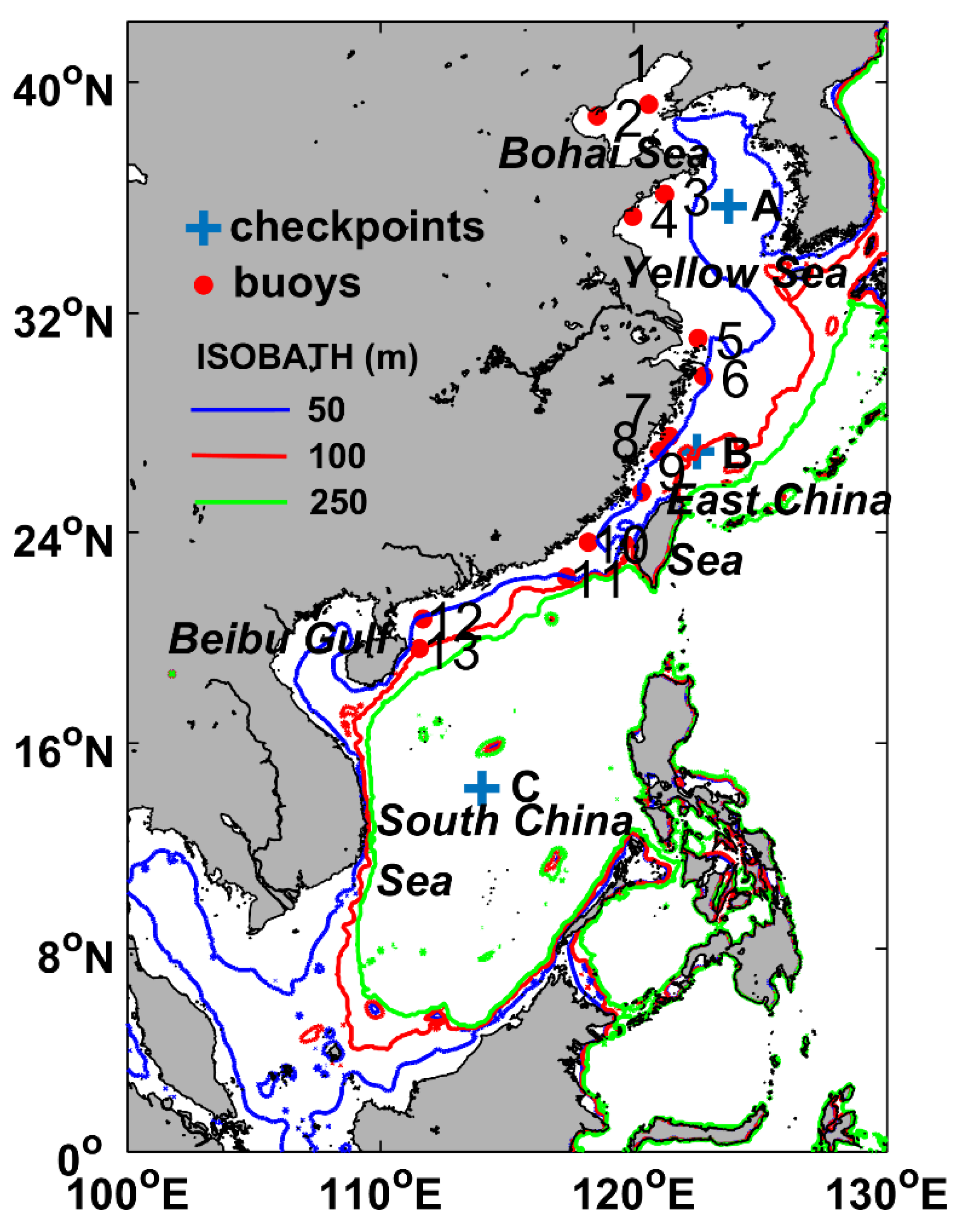
2.1.1. Scatterometer Winds and Buoy Measurements
2.1.2. CFSR Winds
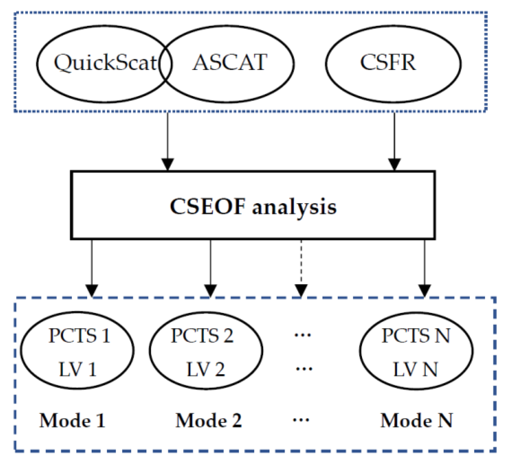
2.2. CSEOF Analysis
3. Results
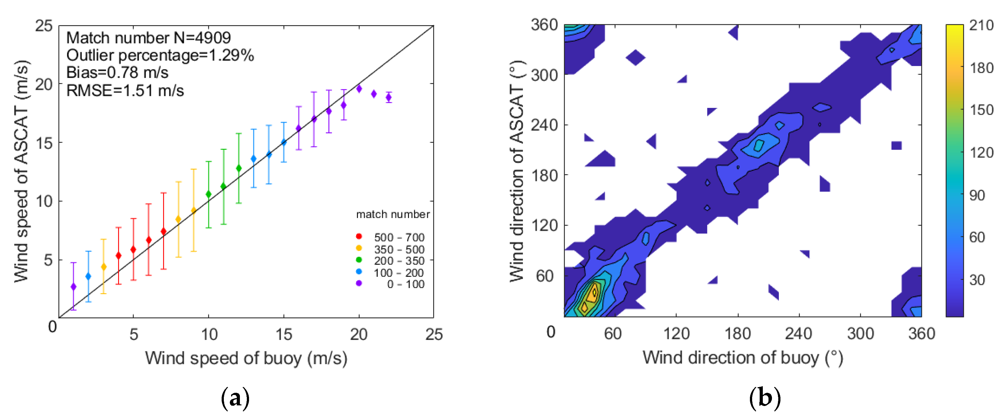
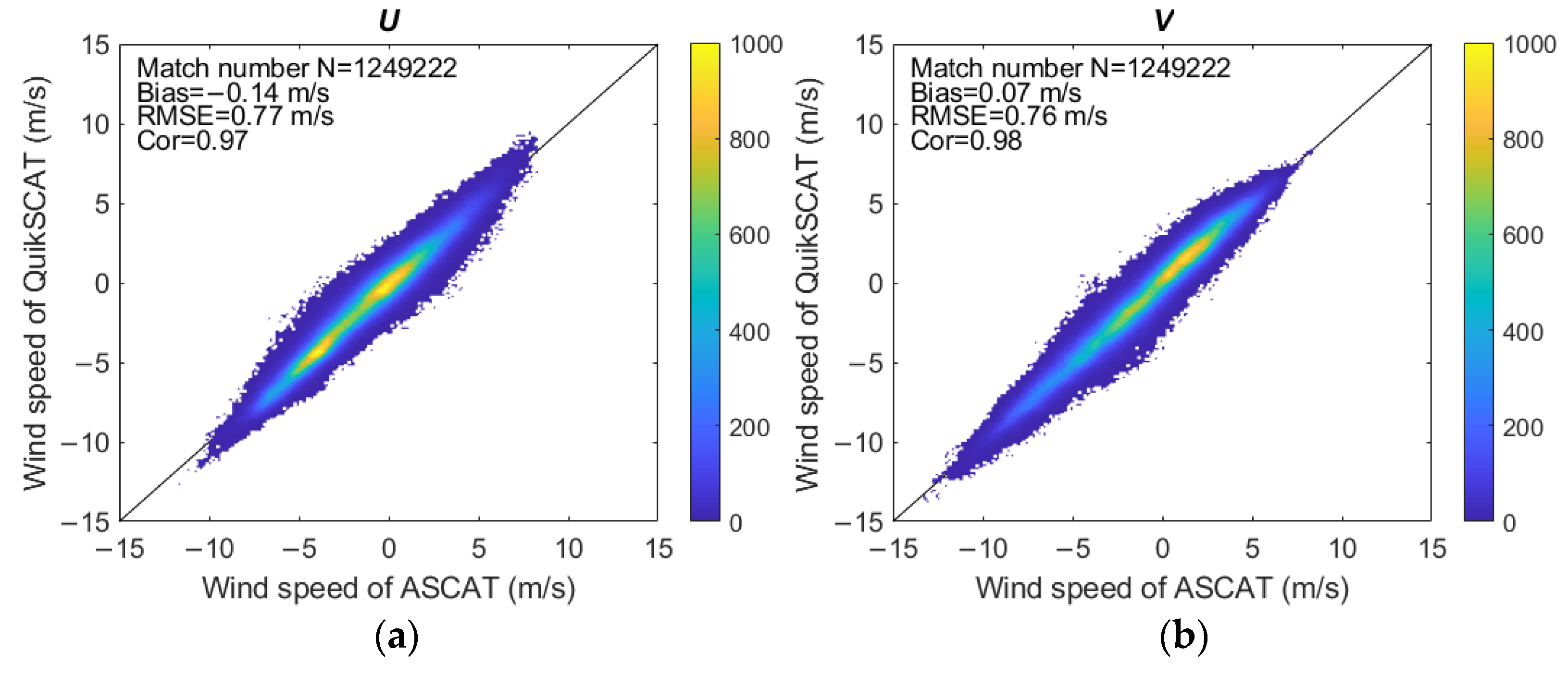
3.1. Validation of Scatterometer Wind Products
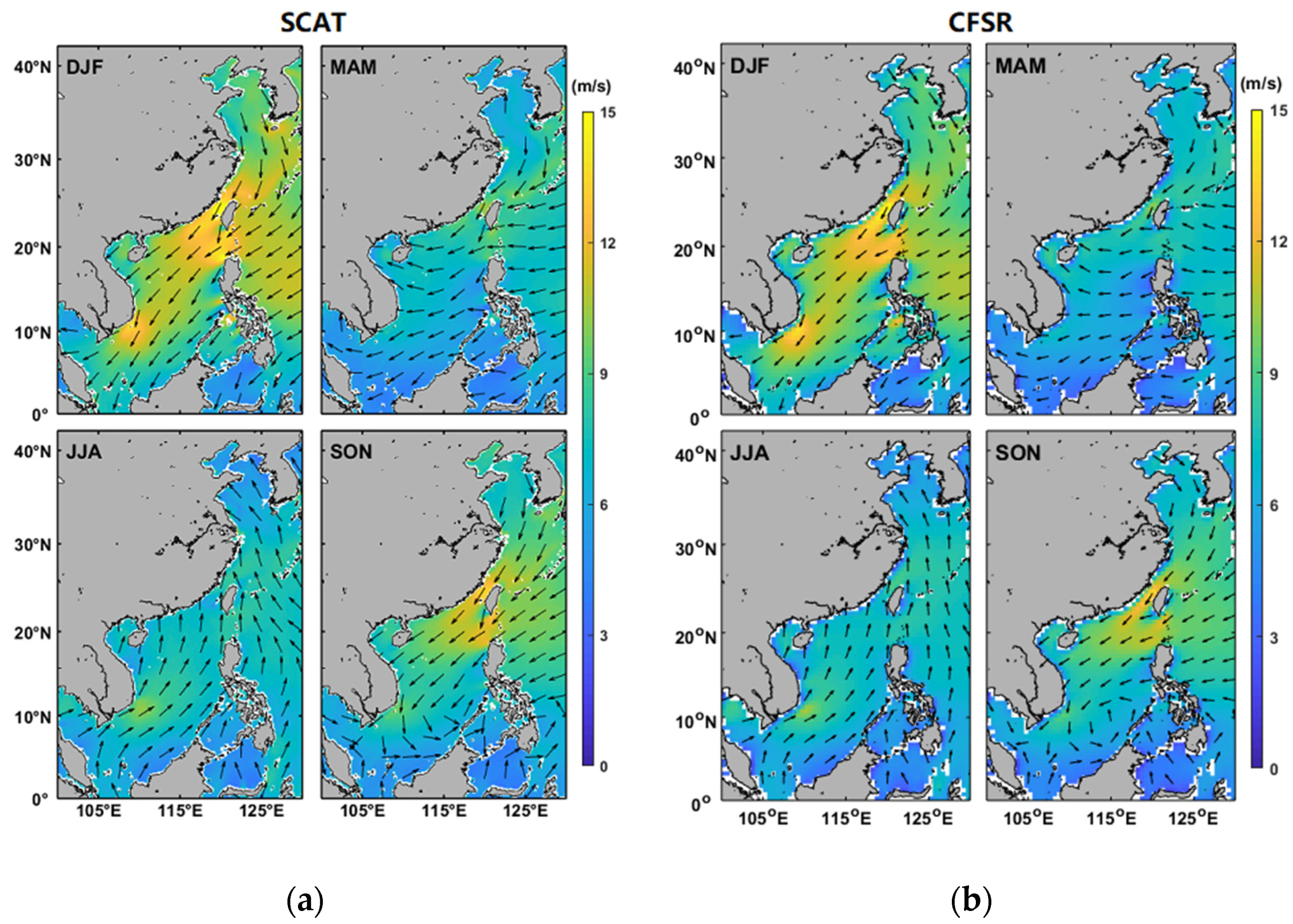
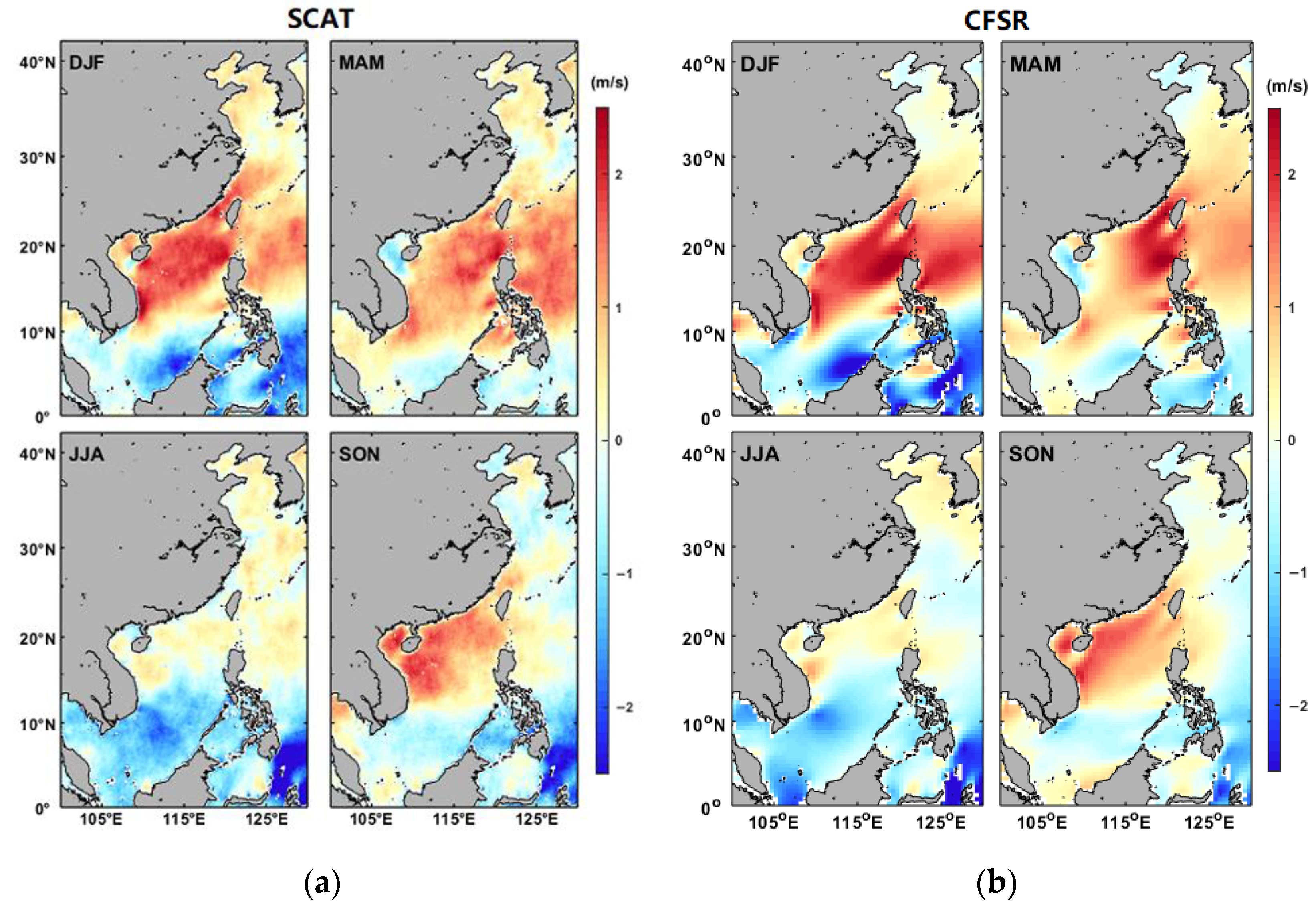
3.2. Seasonal Variation in Wind Speeds
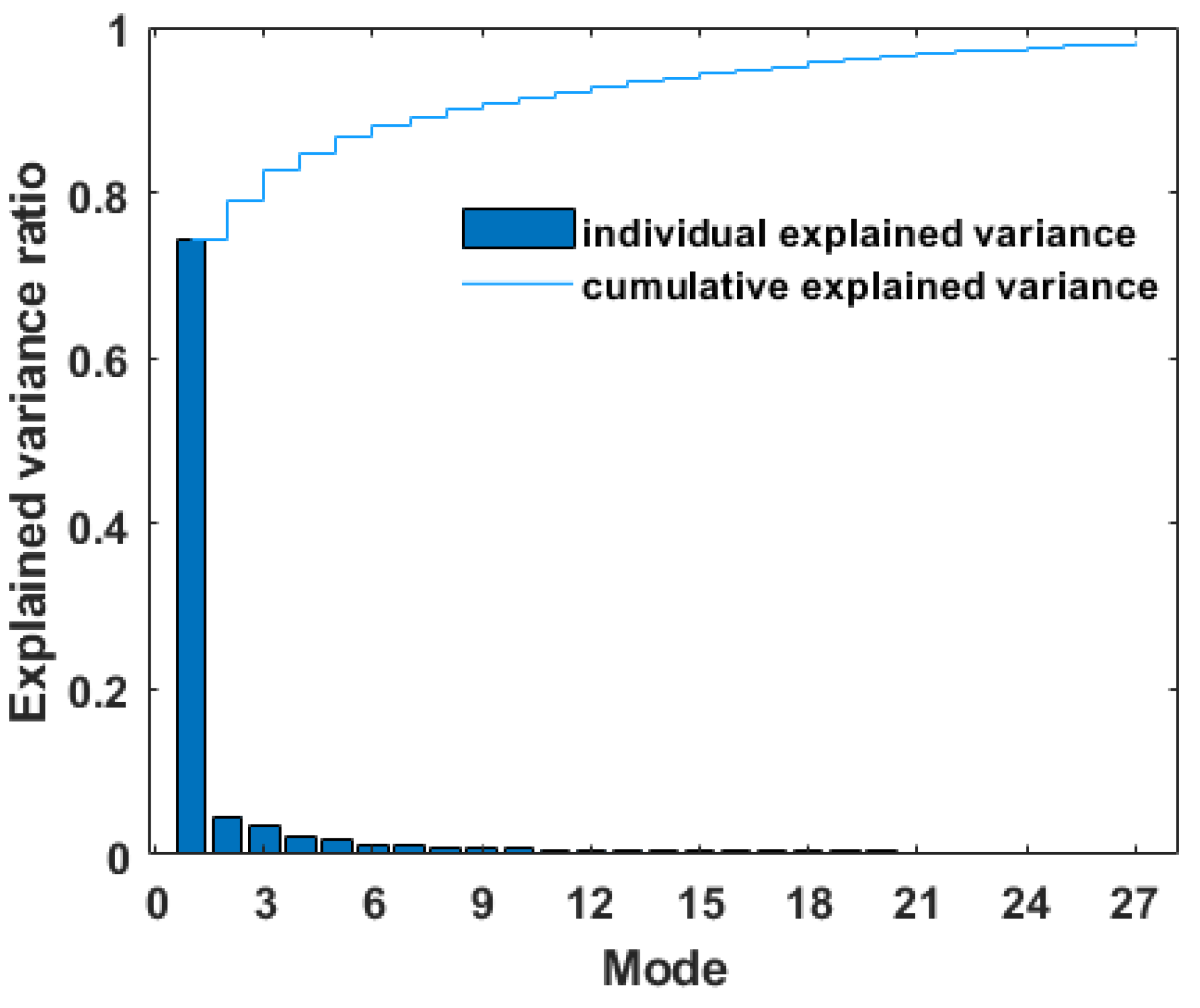
3.3. Modulated Annual Cycle Mode
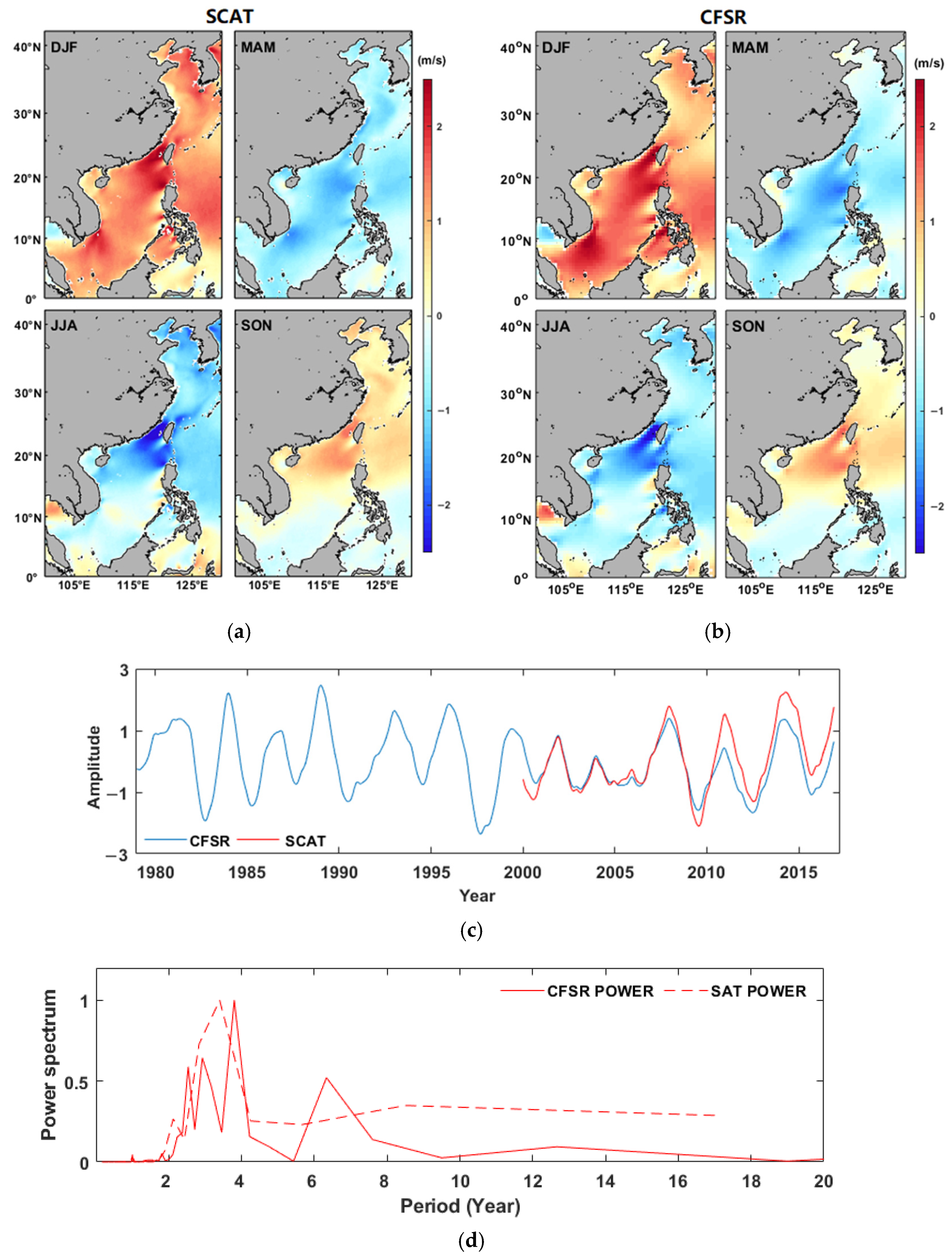
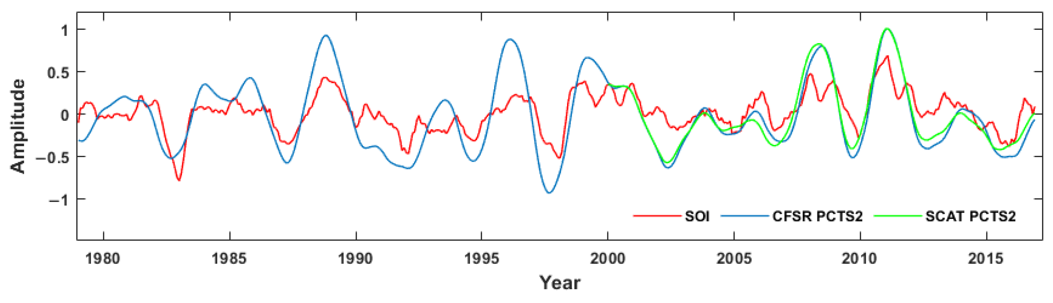
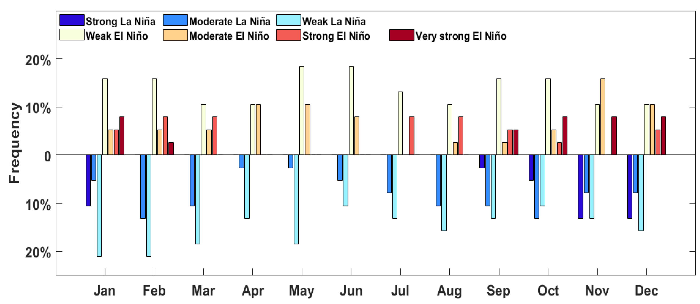
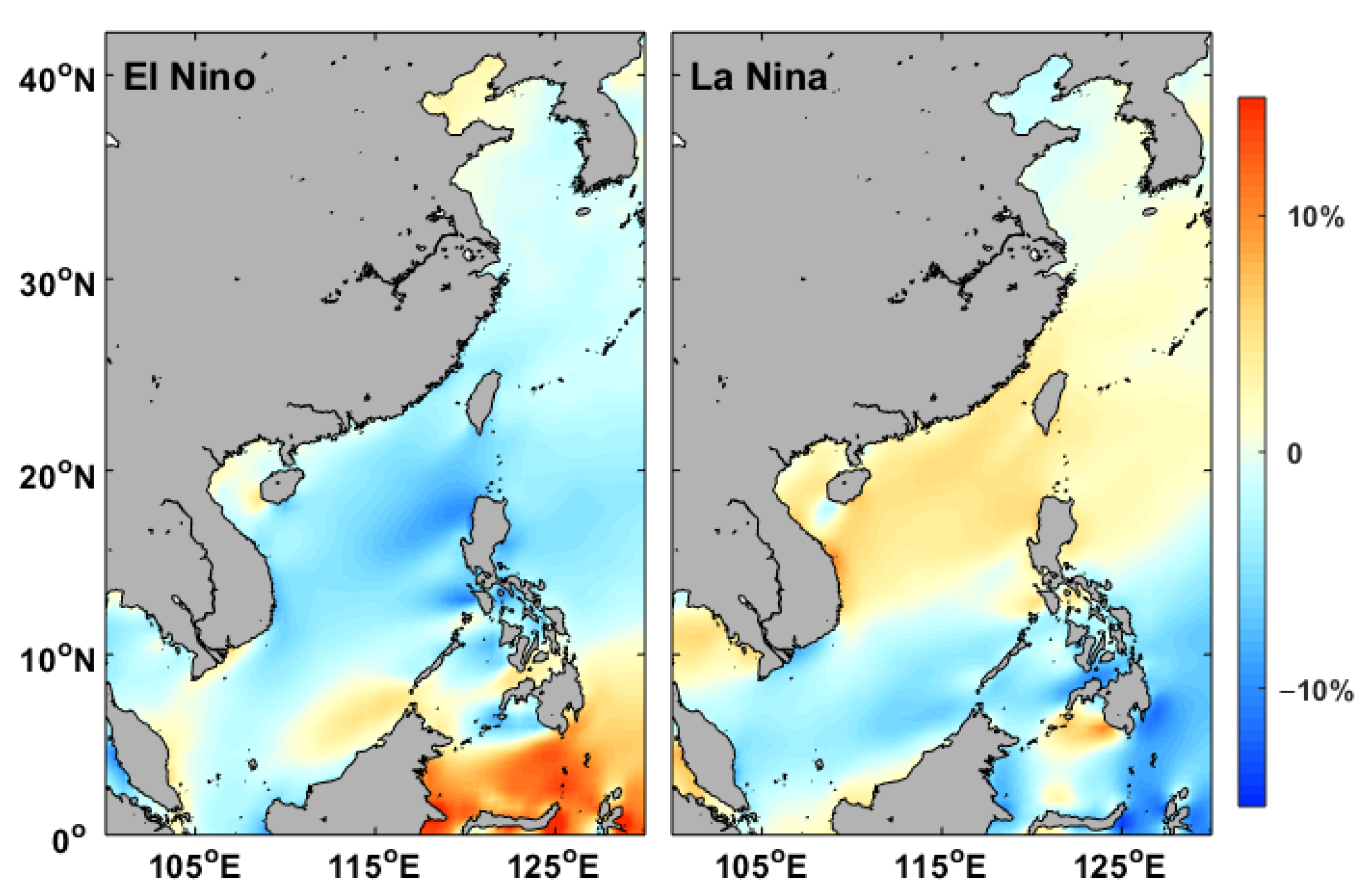
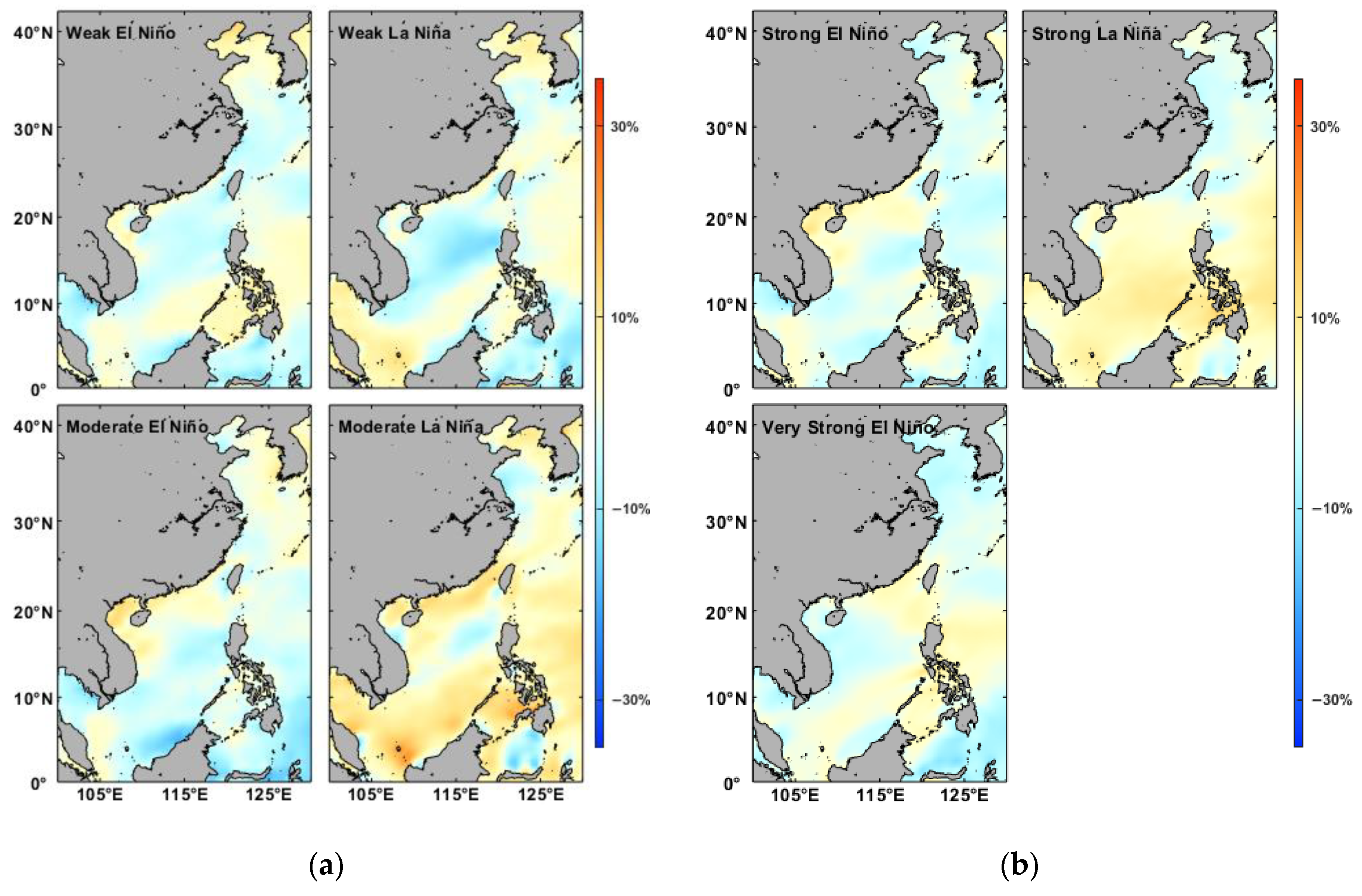
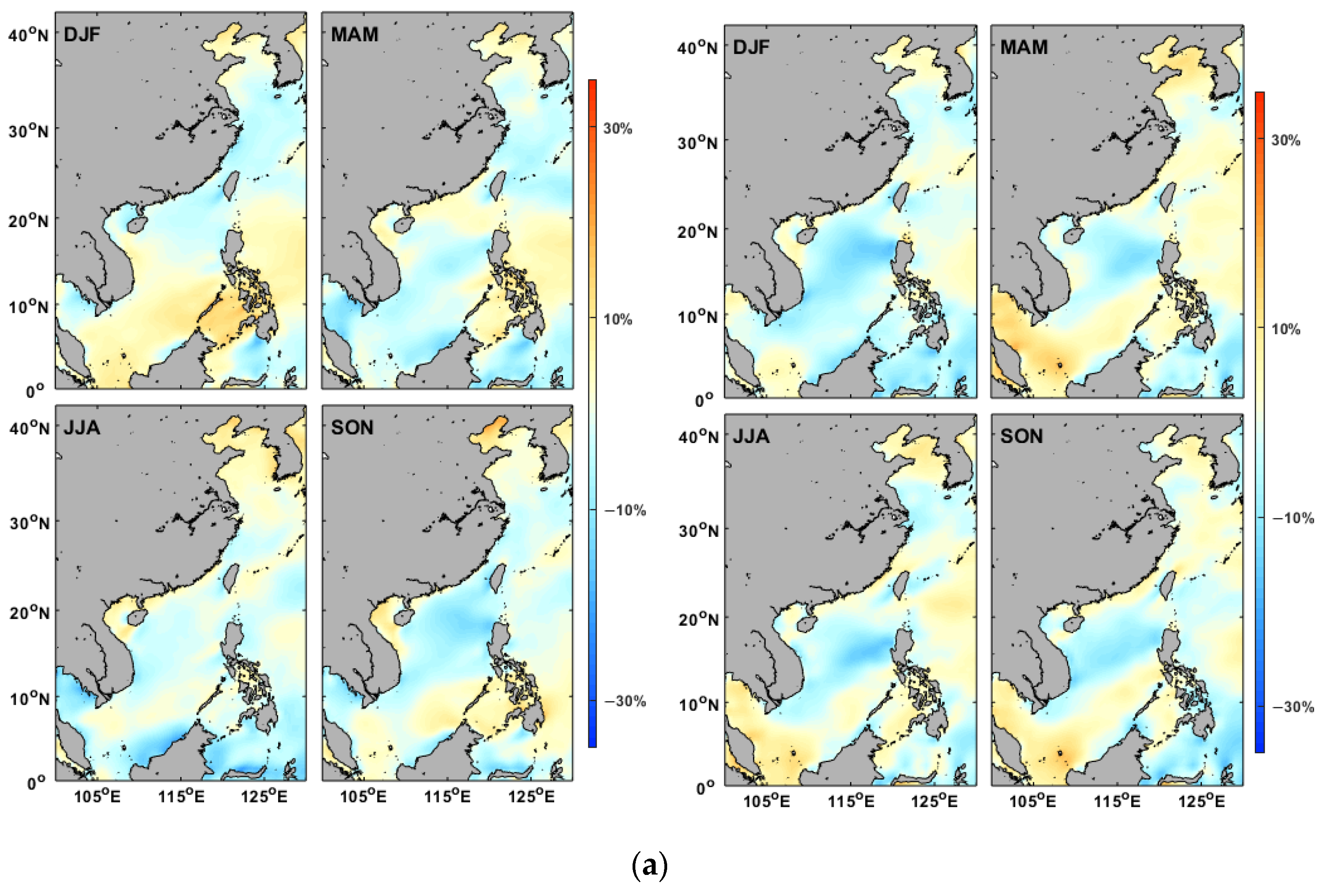
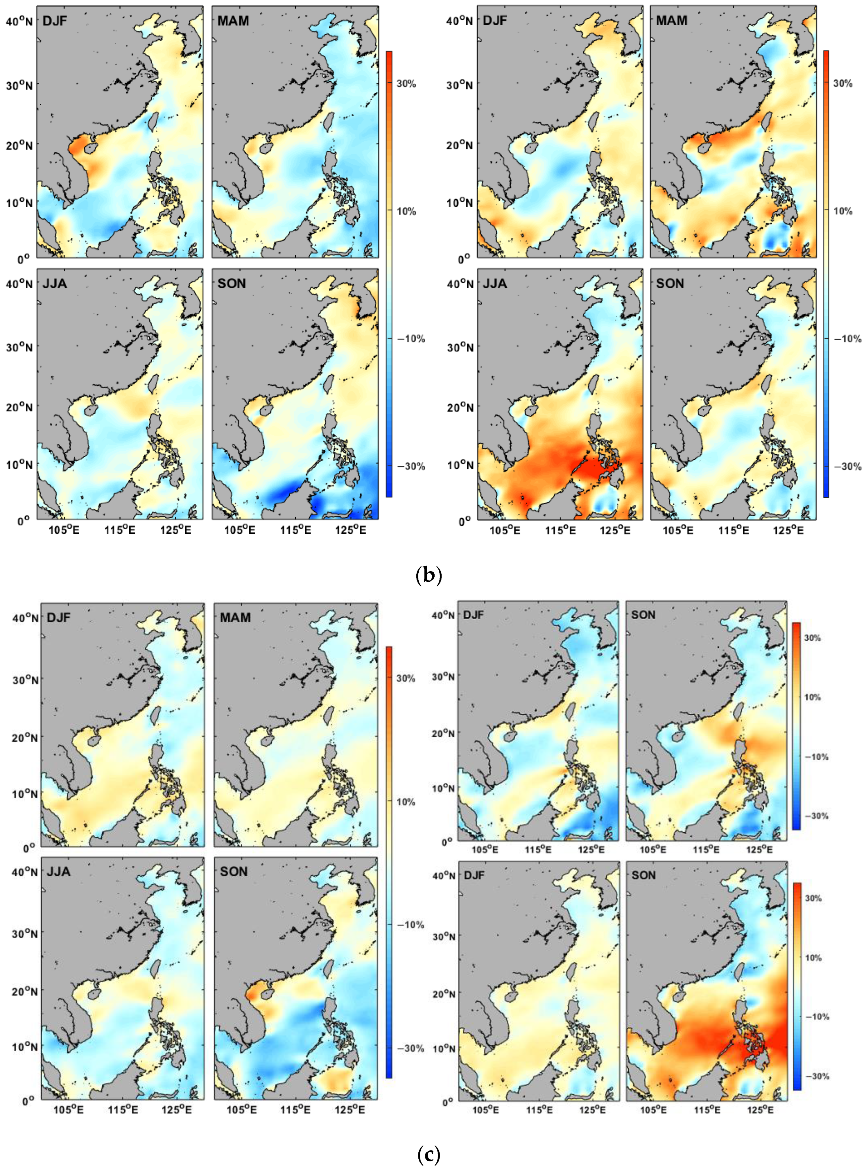
3.4. ENSO Mode
4. Discussion
5. Conclusions
Author Contributions
Funding
Data Availability Statement
Acknowledgments
Conflicts of Interest
Abbreviations
| ASCAT | Advanced Scatterometer |
| CFSR | Climate Forecast System Reanalysis |
| CMEMS | Copernicus Marine Environment Monitoring Service |
| CSEOF | Cyclostationary Empirical Orthogonal Function |
| DJF | December, January, February |
| ENSO | El Nino Southern Oscillation |
| EOF | Empirical Orthogonal Function |
| JJA | June, July, August |
| LV | Loading Vector |
| MAM | March, April, May |
| NWP | Numerical Weather Prediction |
| ONI | Oceanic Niño Index |
| OSCAT | Ocean Scatterometer |
| PCTS | Principal Component Time Series |
| QuikSCAT | Quick Scatterometer |
| RMSE | Root Mean Square Error |
| SAR | Synthetic Aperture Radar |
| SCS | South China Sea |
| SCAT | Scatterometer |
| SOI | Southern Oscillation Index |
| SON | September, October, November |
References
- Zheng, C.; Li, C.; Pan, J.; Liu, M.; Xia, L. An overview of global ocean wind energy resource evaluations. Renew. Sustain. Energy Rev. 2016, 53, 1240–1251. [Google Scholar] [CrossRef]
- Sustainability Development Goals (2016–2030). Available online: https://www.undp.org/sustainable-development-goals (accessed on 1 January 2022).
- Nie, B.; Li, J. Technical potential assessment of offshore wind energy over shallow continent shelf along China coast. Renew. Energy 2018, 128, 391–399. [Google Scholar] [CrossRef] [Green Version]
- Zhang, J.; Zhang, J.; Cai, L.; Ma, L. Energy performance of wind power in China: A comparison among inland, coastal and offshore wind farms. J. Clean. Prod. 2017, 143, 836–842. [Google Scholar] [CrossRef]
- China Daily. Goals for Carbon Peaking, Neutrality. 2020. Available online: https://www.chinadaily.com.cn/a/202010/22/WS5f90c9e4a31024ad0ba80255.html (accessed on 1 January 2022).
- Liu, W.T.; Tang, W.Q.; Xie, X.S. Wind power distribution over the ocean. Geophys. Res. Lett. 2008, 35, L13808. [Google Scholar] [CrossRef] [Green Version]
- Stoffelen, A.; Anderson, D. Scatterometer data interpretation: Estimation and validation of the transfer function CMOD4. J. Geophys. Res. Ocean 1997, 102, 5767–5780. [Google Scholar] [CrossRef]
- Hersbach, H. Comparison of C-band scatterometer CMOD5.N equivalent neutral winds with ECMWF. J. Atmos. Ocean. Technol. 2010, 27, 721–736. [Google Scholar] [CrossRef]
- Wentz, F.J. Measurement of oceanic wind vector using satellite microwave radiometers. IEEE Trans. Geosci. Remote Sens. 1992, 30, 960–972. [Google Scholar] [CrossRef]
- Zhang, L.; Shi, H.; Wang, Z.; Yu, H.; Yin, X.; Liao, Q. Comparison of wind speeds from spaceborne microwave radiometers with in situ observations and ECMWF data over the global ocean. Remote Sens. 2018, 10, 425. [Google Scholar] [CrossRef] [Green Version]
- Xu, Q.; Lin, H.; Li, X.; Zuo, J.; Zheng, Q.; Pichel, W.G.; Liu, Y. Assessment of an analytical model for sea surface wind speed retrieval from spaceborne SAR. Int. J. Remote Sens. 2010, 31, 993–1008. [Google Scholar] [CrossRef]
- Zhang, B.; Mouche, A.; Lu, Y.; Perrie, W.; Zhang, G.; Wang, H. A geophysical model function for wind speed retrieval from C-band HH-polarized synthetic aperture radar. IEEE Geosci. Remote Sens. Lett. 2019, 16, 1521–1525. [Google Scholar] [CrossRef]
- Yang, X.; Li, X.; Pichel, W.G.; Li, Z. Comparison of ocean surface winds from ENVISAT ASAR, MetOp ASCAT scatterometer, buoy measurements, and NOGAPS model. IEEE Trans. Geosci. Remote Sens. 2011, 49, 4743–4750. [Google Scholar] [CrossRef]
- Pimenta, F.; Kempton, W.; Garvine, R. Combining meteorological stations and satellite data to evaluate the offshore wind power resource of Southeastern Brazil. Renew. Energy 2008, 33, 2375–2387. [Google Scholar] [CrossRef]
- Furevik, B.R.; Sempreviva, A.M.; Cavaleri, L.; Lefèvre, J.-M.; Transerici, C. Eight years of wind measurements from scatterometer for wind resource mapping in the Mediterranean Sea. Wind Energy 2011, 14, 355–372. [Google Scholar] [CrossRef] [Green Version]
- Karagali, I.; Peña, A.; Badger, M.; Hasager, C.B. Wind characteristics in the North and Baltic Seas from the QuikSCAT satellite. Wind Energy 2014, 17, 123–140. [Google Scholar] [CrossRef]
- Jiang, D.; Zhuang, D.; Huang, Y.; Wang, J.; Fu, J. Evaluating the spatio-temporal variation of China’s offshore wind resources based on remotely sensed wind field data. Renew. Sustain. Energy Rev. 2013, 24, 142–148. [Google Scholar] [CrossRef]
- Wang, Z.; Duan, C.; Dong, S. Long-term wind and wave energy resource assessment in the South China sea based on 30-year hindcast data. Ocean Eng. 2018, 163, 58–75. [Google Scholar] [CrossRef]
- Benazzouz, A.; Mabchour, H.; El Had, K.; Zourarah, B.; Mordane, S. Offshore wind energy resource in the Kingdom of Morocco: Assessment of the seasonal potential variability based on satellite data. J. Mar. Sci. Eng. 2020, 9, 31. [Google Scholar] [CrossRef]
- Capps, S.B.; Zender, C.S. Estimate global ocean wind power potential from QuikSCAT observations, accounting for turbine characteristics and siting. J. Geophys. Res. 2010, 115, 12679–12691. [Google Scholar] [CrossRef]
- Kumar, S.V.A.; Nagababu, G.; Sharma, R.; Kumar, R. Synergetic use of multiple scatterometers for offshore wind energy potential assessment. Ocean Eng. 2020, 196, 106745. [Google Scholar] [CrossRef]
- Guo, Q.; Xu, X.; Zhang, K.; Li, Z.; Huang, W.; Mansaray, L.; Liu, W.; Wang, X.; Gao, J.; Huang, J. Assessing global ocean wind energy resources using multiple satellite data. Remote Sens. 2018, 10, 100. [Google Scholar] [CrossRef] [Green Version]
- Hasager, C.B.; Mouche, A.; Badger, M.; Bingöl, F.; Karagali, I.; Driesenaar, T.; Stoffelen, A.; Peña, A.; Longépé, N. Offshore wind climatology based on synergetic use of Envisat ASAR, ASCAT and QuikSCAT. Remote Sens. Environ. 2015, 156, 247–263. [Google Scholar] [CrossRef]
- Chang, R.; Zhu, R.; Badger, M.; Hasager, C.; Xing, X.; Jiang, Y. Offshore wind resources assessment from multiple satellite data and WRF modeling over South China Sea. Remote Sens. 2015, 7, 467–487. [Google Scholar] [CrossRef] [Green Version]
- Nezhad, M.M.; Neshat, M.; Groppi, D.; Marzialetti, P.; Heydari, A.; Sylaios, G.; Garcia, D.A. A primary offshore wind farm site assessment using reanalysis data: A case study for Samothraki island. Renew. Energy 2021, 172, 667–679. [Google Scholar] [CrossRef]
- Nezhad, M.M.; Neshat, M.; Heydari, A.; Razmjoo, A.; Piras, G.; Garcia, D.A. A new methodology for offshore wind speed assessment integrating Sentinel-1, ERA-Interim and in-situ measurement. Renew. Energy 2021, 172, 1301–1313. [Google Scholar] [CrossRef]
- Ge, L.; Uchida, T.; Ohya, Y. Spatial and annual variation of offshore wind resource in China. Energy Power Eng. 2014, 6, 111–118. [Google Scholar] [CrossRef] [Green Version]
- Chang, T.-J.; Chen, C.-L.; Tu, Y.-L.; Yeh, H.-T.; Wu, Y.-T. Evaluation of the climate change impact on wind resources in Taiwan Strait. Energy Convers. Manag. 2015, 95, 435–445. [Google Scholar] [CrossRef]
- Wen, Y.; Kamranzad, B.; Lin, P. Assessment of long-term offshore wind energy potential in the south and southeast coasts of China based on a 55-year dataset. Energy 2021, 224, 120225. [Google Scholar] [CrossRef]
- Hamlington, B.; Hamlington, P.; Collins, S.; Alexander, S.; Kim, K.-Y. Effects of climate oscillations on wind resource variability in the United States. Geophys. Res. Lett. 2015, 42, 145–152. [Google Scholar] [CrossRef] [Green Version]
- Watts, D.; Durán, P.; Flores, Y. How does El Niño Southern Oscillation impact the wind resource in Chile? A techno-economical assessment of the influence of El Niño and La Niña on the wind power. Renew. Energy 2017, 103, 128–142. [Google Scholar] [CrossRef]
- Yu, L.; Zhong, S.; Bian, X.; Heilman, W.E. The interannual variability of wind energy resources across China and its relationship to large-scale circulation changes. Int. J. Climatol. 2019, 39, 1684–1699. [Google Scholar] [CrossRef]
- Zhang, G.; Xu, Q.; Gong, Z.; Cheng, Y.; Wang, L.; Ji, Q. Annual and interannual variability of scatterometer ocean surface wind over the South China Sea. J. Ocean Univ. China 2014, 13, 191–197. [Google Scholar] [CrossRef]
- Verhoef, A.; Stoffelen, A. ASCAT Wind Validation Report, OSI SAF Report, SAF/OSI/CDOP3/KNMI/TEC/RP/326; Royal Netherlands Meteorological Institute: De Bilt, The Netherlands, 2018. [Google Scholar]
- Ricciardulli, L.; National Center for Atmospheric Research Staff. The Climate Data Guide: QuikSCAT: Near Sea-Surface Wind Speed and Direction. 2016. Available online: https://climatedataguide.ucar.edu/climate-data/quikscat-near-sea-surface-wind-speed-and-direction (accessed on 1 January 2022).
- Xu, Q.; Zhang, G.; Cheng, Y.; Ji, Q.; Wang, L.; Zhao, Y. Wind resource estimation using QuikSCAT ocean surface winds. In Proceedings of the International Offshore and Polar Engineering Conference, Maui, HI, USA, 19–24 June 2011; pp. 506–510. [Google Scholar]
- Chelliah, M.; Ebisuzaki, W.; Weaver, S.; Kumar, A. Evaluating the tropospheric variability in National Centers for Environmental Prediction’s climate forecast system reanalysis. J. Geophys. Res. Atmos. 2011, 116, D17107. [Google Scholar] [CrossRef]
- Saha, S.; Moorthi, S.; Pan, H.-L.; Wu, X.; Wang, J.; Nadiga, S.; Tripp, P.; Kistler, R.; Woollen, J.; Behringer, D.; et al. The NCEP climate forecast system reanalysis. Bull. Am. Meteorol. Soc. 2010, 91, 1015–1058. [Google Scholar] [CrossRef]
- Saha, S.; Moorthi, S.; Wu, X.; Wang, J.; Nadiga, S.; Tripp, P.; Behringer, D.; Hou, Y.-T.; Chuang, H.-Y.; Iredell, M.; et al. The NCEP climate forecast system version 2. J. Clim. 2014, 27, 2185–2208. [Google Scholar] [CrossRef]
- Hsu, S.; Meindl, E.A.; Gilhousen, D.B. Determining the power-law wind-profile exponent under near-neutral stability conditions at sea. J. Appl. Meteorol. 1994, 33, 757–765. [Google Scholar] [CrossRef] [Green Version]
- Chen, Y.; Zhao, Y.; Zhang, B.; Yang, L.; Wu, S.; Song, S. The study of the relations of wind velocity at different heights over the sea. Mar. Sci. 1989, 3, 27–31. [Google Scholar]
- Panofsky, H.A.; Dutton, J.A. Atmospheric Turbulence; John Wiley: New York, NY, USA, 1984. [Google Scholar]
- Hamlington, B.D.; Leben, R.R.; Nerem, R.S.; Han, W.; Kim, K.-Y. Reconstructing sea level using cyclostationary empirical orthogonal functions. J. Geophys. Res. Ocean 2011, 116, C12015. [Google Scholar] [CrossRef] [Green Version]
- Cheng, Y.; Plag, H.-P.; Hamlington, B.D.; Xu, Q.; He, Y. Regional sea level variability in the Bohai Sea, Yellow Sea, and East China Sea. Cont. Shelf Res. 2015, 111, 95–107. [Google Scholar] [CrossRef]
- Cheng, Y.; Hamlington, B.; Plag, H.-P.; Xu, Q. Influence of ENSO on the variation of annual sea level cycle in the South China Sea. Ocean Eng. 2016, 126, 343–352. [Google Scholar] [CrossRef]
- Bentamy, A.; Croize-Fillon, D.; Perigaud, C. Characterization of ASCAT measurements based on buoy and QuikSCAT wind vector observations. Ocean Sci. 2008, 4, 265–274. [Google Scholar] [CrossRef] [Green Version]
- Ricciardulli, L.; Wentz, F.J. A scatterometer geophysical model function for climate-quality winds: QuikSCAT Ku-2011. J. Atmos. Ocean. Technol. 2015, 32, 1829–1846. [Google Scholar] [CrossRef]
- Yang, X.; Li, X.; Zheng, Q.; Gu, X.; Pichel, W.G.; Li, Z. Comparison of ocean-surface winds retrieved from QuikSCAT scatterometer and radarsat-1 SAR in offshore waters of the US west coast. IEEE Geosci. Remote Sens. Lett. 2010, 8, 163–167. [Google Scholar] [CrossRef]
- Xu, Q.; Li, Y.; Li, X.; Zhang, Z.; Cao, Y.; Cheng, Y. Impact of ships and ocean fronts on coastal sea surface wind measurements from the advanced scatterometer. IEEE J. Sel. Top. Appl. Earth Obs. Remote Sens. 2018, 11, 2162–2169. [Google Scholar] [CrossRef]
- Aboobacker, V.M.; Shanas, P.R.; Veerasingam, S.; Al-Ansari, E.M.A.S.; Sadooni, F.N.; Vethamony, P. Long-term assessment of onshore and offshore wind energy potentials of Qatar. Energies 2021, 14, 1178. [Google Scholar] [CrossRef]
- Shanas, P.; Aboobacker, V.; Albarakati, A.M.; Zubier, K.M. Climate driven variability of wind-waves in the Red Sea. Ocean Model. 2017, 119, 105–117. [Google Scholar] [CrossRef]


| Locations | U | V | ||
|---|---|---|---|---|
| Bias (m/s) | R | Bias (m/s) | R | |
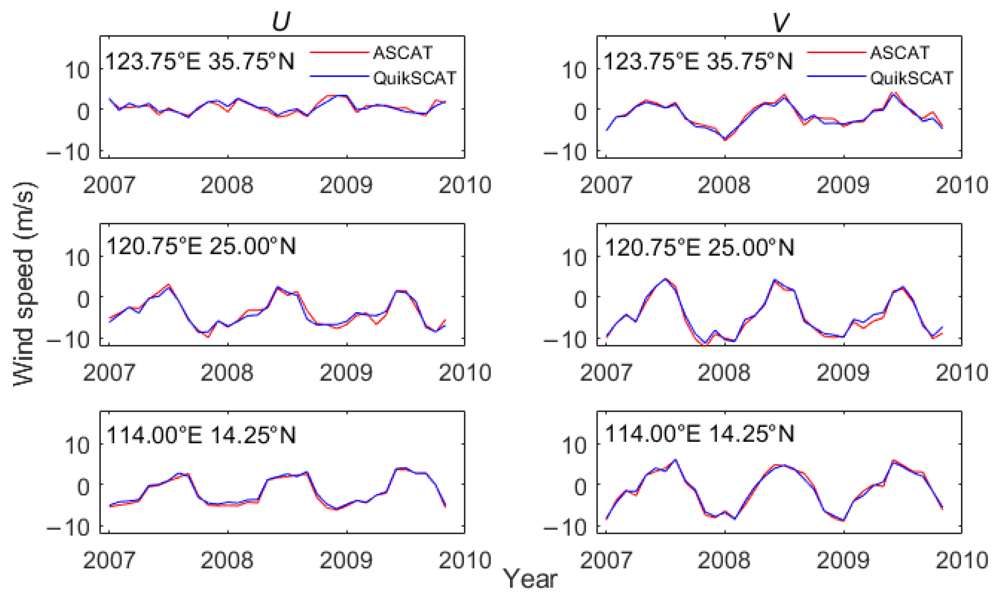
| A (123.75°E, 35.75°N) | −0.10 | 0.89 | 0.28 | 0.97 |
| B (120.75°E, 25°N) | 0.09 | 0.96 | −0.43 | 0.99 |
| C (114°E, 14.25°N) | −0.34 | 0.99 | 0.01 | 0.99 |
| ONI Range | Intensity | ONI Range | Intensity |
|---|---|---|---|
| Weak El Niño | Weak La Niña | ||
| Moderate El Niño | Moderate La Niña | ||
| Strong El Niño | Strong La Niña | ||
| Very strong El Niño | Very Strong La Niña |
Publisher’s Note: MDPI stays neutral with regard to jurisdictional claims in published maps and institutional affiliations. |
© 2022 by the authors. Licensee MDPI, Basel, Switzerland. This article is an open access article distributed under the terms and conditions of the Creative Commons Attribution (CC BY) license (https://creativecommons.org/licenses/by/4.0/).
Share and Cite
Xu, Q.; Li, Y.; Cheng, Y.; Ye, X.; Zhang, Z. Impacts of Climate Oscillation on Offshore Wind Resources in China Seas. Remote Sens. 2022, 14, 1879. https://doi.org/10.3390/rs14081879
Xu Q, Li Y, Cheng Y, Ye X, Zhang Z. Impacts of Climate Oscillation on Offshore Wind Resources in China Seas. Remote Sensing. 2022; 14(8):1879. https://doi.org/10.3390/rs14081879
Chicago/Turabian StyleXu, Qing, Yizhi Li, Yongcun Cheng, Xiaomin Ye, and Zenghai Zhang. 2022. "Impacts of Climate Oscillation on Offshore Wind Resources in China Seas" Remote Sensing 14, no. 8: 1879. https://doi.org/10.3390/rs14081879