Article

Exploiting Graph and Geodesic Distance Constraint for Deep Learning-Based Visual Odometry

1
Guangdong Key Laboratory of Urban Informatics, Shenzhen University, Shenzhen 518060, China
2
College of Electronics and Information Engineering, Shenzhen University, Shenzhen 518060, China
3
College of Civil and Transportation Engineering, Shenzhen University, Shenzhen 518060, China
4
School of Computer Science and Technology, Dongguan University of Technology, Dongguan 523808, China
5
Shenzhen University Branch, Shenzhen Institute of Artificial Intelligence and Robotics for Society, Shenzhen 518060, China
*
Author to whom correspondence should be addressed.
Remote Sens. 2022, 14(8), 1854; https://doi.org/10.3390/rs14081854
Submission received: 2 March 2022 / Revised: 1 April 2022 / Accepted: 9 April 2022 / Published: 12 April 2022
(This article belongs to the Topic Artificial Intelligence in Sensors)

Abstract

:
Visual odometry is the task of estimating the trajectory of the moving agents from consecutive images. It is a hot research topic both in robotic and computer vision communities and facilitates many applications, such as autonomous driving and virtual reality. The conventional odometry methods predict the trajectory by utilizing the multiple view geometry between consecutive overlapping images. However, these methods need to be carefully designed and fine-tuned to work well in different environments. Deep learning has been explored to alleviate the challenge by directly predicting the relative pose from the paired images. Deep learning-based methods usually focus on the consecutive images that are feasible to propagate the error over time. In this paper, graph loss and geodesic rotation loss are proposed to enhance deep learning-based visual odometry methods based on graph constraints and geodesic distance, respectively. The graph loss not only considers the relative pose loss of consecutive images, but also the relative pose of non-consecutive images. The relative pose of non-consecutive images is not directly predicted but computed from the relative pose of consecutive ones. The geodesic rotation loss is constructed by the geodesic distance and the model regresses a Lie algebra so(3) (3D vector). This allows a robust and stable convergence. To increase the efficiency, a random strategy is adopted to select the edges of the graph instead of using all of the edges. This strategy provides additional regularization for training the networks. Extensive experiments are conducted on visual odometry benchmarks, and the obtained results demonstrate that the proposed method has comparable performance to other supervised learning-based methods, as well as monocular camera-based methods. The source code and the weight are made publicly available.

Graphical Abstract

1. Introduction

Visual odometry (VO) is the task of estimating the trajectory of mobile agents (e.g., robots, vehicles, and unmanned aerial vehicles (UAVs)) from image sequences. It is one of the fundamental and important remote sensing methods in autonomous driving, photogrammetry, and virtual/augmented reality (VR, AR) applications. In the past few decades, visual odometry has attracted significant interest in both robotics and computer vision communities [1]. Visual odometry was first proposed in 2004 by Nister [2] for the navigation of autonomous ground vehicles. Later, monocular visual navigation was achieved for autonomous micro helicopters [3]. Visual odometry is also a promising supplement to other localization technologies, such as inertial measurement unit (IMU), global positioning system (GPS), LiDAR and ultrasonic rangefinder especially in GPS-denied environments, such as tunnels, underwater, and indoor scenarios [4,5,6]. The IMU is a lightweight, low-cost sensor that can improve the motion tracking performance of visual sensors by integrating the IMU measurements. The ultrasonic rangefinder can provide the backup for the LiDAR rangefinder, due to the LiDAR beam being narrow. Fusing the advantages of different remote sensing techniques can enhance the reliability of the system. The performance of visual odometry is important for various artificial intelligence applications.
Although numerous conventional visual odometry or simultaneous localization and mapping (SLAM) methods have shown promising results under the ideal environment, they still face both external and internal challenges. The external challenges refer to harsh environments of illumination changes, textureless surfaces, and dynamic objects scenes. While the internal challenge is that different cameras need to be precisely calibrated for better performance. To alleviate these problems, deep learning has been utilized [7,8,9]. Estimating the relative pose is an important component for VO/SLAM. The relative pose describes the translation and rotation between frames. Deep learning-based methods directly predict the relative pose by sequentially feeding the paired images into the deep neural networks. Deep learning-based methods construct a generic data-driven model and avoid effort on specifying the full knowledge about physical and mathematical rules [10,11,12]. Long short-term memory (LSTM) has also been incorporated to leverage the spatial correspondences of consecutive images for visual odometry due to its internal advantage for sequential information processing [7,13]. The networks are trained with loss that is designed based on the deviation between the predicted and the real relative poses. However, the existing methods usually predict the relative pose from two consecutive images of the images sequence, in which errors are accumulated over time. To alleviate the problem, a graph loss is designed in the paper to utilize the constraints of all the overlapped images in a tiny sequence. The relative pose losses of both consecutive and non-consecutive images are considered. The relative pose of non-consecutive images is not directly predicted but computed from the relative pose of consecutive images. This approach provides additional regularization for training the networks. Figure 1 shows the basic idea of the proposed method and the difference with other deep learning-based methods. Moreover, a novel geodesic rotation loss is formulated based on the real rotation change in 3D space. Instead of comparing the distances of the predicted and the real rotations in a certain representation, the orientation difference from the predicted to the real rotations is directly computed.
The main contributions of this paper are as follows:
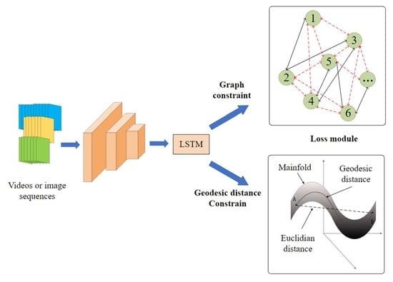
  • A graph loss is proposed to fully exploit the constraints of a tiny image sequence to replace the conventional loss module based on two consecutive images, which can alleviate the accumulating errors in visual odometry. Moreover, the proposed graph loss leads to more constraints to regularize the network.
  • A new representation of rotation loss is designed based on the geodesic distance, which is more robust than the usual methods that use the angles difference in Euclidean distance.
  • Extensive experiments are conducted to demonstrate the superiority of the proposed losses. Furthermore, the effects of different sliding window sizes and sequence overlapping are also analyzed.
The remainder of the paper is organized as follows: Section 2 presents an overview of related works on visual odometry. Section 3 describes the proposed method and the loss functions. The experiments are presented in Section 4. Section 5 discusses the effects in different experimental settings. Section 6 concludes the paper.

2. Related Work

The various approaches and frameworks proposed for visual odometry can be divided into two categories: geometry-based methods and learning-based methods.

2.1. Geometry-Based Methods

Geometry-based methods estimate the relative pose between frame-to-frame based on the stereo view geometry. A typical pipeline of the geometry-based method contains camera calibration [14], feature extraction [15], feature matching, outlier removal, and optimization module [16,17,18]. Based on this theory, numerous visual odometry algorithms and SLAM systems have been created, demonstrating exceptional performance [19], such as VINS-MONO [20], ORB-SLAM3 [21], and Kimera-VIO [22]. These methods are robust and versatile visual or visual-inertial odometry methods that utilize the image data and other sensor data. Zhang et al. [23] proposed a series of optimal methods that made 3D reconstruction and mapping systems more robust and accurate. Generally, the two dominant geometry-based methods are feature-based methods and direct methods. The feature-based methods use various feature detectors, including FAST [24], SURF [25], BRIEF [26], and corner detectors [27], to detect the salient features. The feature point tracker is used to track these feature points in the next image of the same sequence. Mono-SLAM [28] simultaneously estimates the camera motion and the 3D structure of an unknown environment in real-time. LIBVISO2 [29] employs multi-view geometry to estimate relative pose by extracting and tracking the salient feature points. One of the most successful and classical SLAM systems is ORB-SLAM2 [30] that was adapted to maintain a feature map for drift correction along with pose estimation. However, the sparse feature-based methods are computationally expensive and do not utilize the information of the whole image.
The direct methods utilize all the pixels and optimize geometry errors for pose estimation between consecutive images under the assumption of photometric consistency [31]. To improve the computational efficiency, the Direct Sparse Odometry (DSO) [32] adopted sparse and direct methods for the monocular camera and demonstrated robustness for photometric consistency. Although many geometry-based methods have shown good performance in good environments, they tend to fail in textureless environments or different illuminations.

2.2. Deep Learning-Based Methods

Motivated by the good performance in object detection and classification [33,34,35,36], deep learning techniques have been introduced to address the problems of traditional camera location methods [37]. K. R. Konda et al. [38] formulated visual odometry as a classification problem. They were the first to apply deep learning methods to visual odometry. The deep learning model was used to predict the velocity and direction with estimated depth from stereo images due to the effective feature representation of the deep learning model [39,40]. The PoseNet [41] considers the camera relocation as a pose regression problem; a convolutional neural network (CNN) built on the GoogLeNet model is used to regress the six degrees of freedom (6-DoF) camera pose from a single RGB image in an end-to-end manner. The KFNet improved the learning-based camera re-localization method by incorporating Kalman filtering [42].
In [43], an image localization has been proposed based on a deep learning method with the pose correction by matching the map inferred from images and local map extract from 3D map. The main disadvantage of this method is that it needs to be re-trained or at least fine-tuned for a new environment, limiting its widespread applications. To address this issue, frame-to-frame Ego-Motion estimation based on CNN was proposed in [44], which achieved robust performance under the challenging scene. However, it is a time-consuming process since the model takes dense optical flow rather than RGB image data as input. Flowdometry [45] cast the visual odometry as a regression problem using the FlowNet [46] to extract the optical flow information and a fully connected layer to directly predict camera translation and rotation. DeepVO [7] regarded visual odometry as a sequential modeling problem and fed image sequences or videos into a network designed based on CNN and recurrent neural network (RNN) in an end-to-end framework. ESP-VO [47] presented a sequence-to-sequence probabilistic visual odometry framework based on DeepVO and predicted the poses and uncertainties of image sequences or videos. M. R. U. Saputra et al. [8] presented a curriculum learning strategy for learning the geometry of monocular visual odometry and constructed geometry-aware objective function by jointly optimizing relative and composite transformations over small windows. Recently, some unsupervised learning-based VO methods have also achieved comparable performances. SC-Sfmlearner [48] achieved the scale consistent on a long video sequence by geometry consistency loss and provided full camera trajectory. TrajNet [49] proposed a novel pose-to-trajectory constraint and improved the view reconstruction constraint to constrain the training process. The above-mentioned methods utilize stereo images and perform depth estimation jointly with visual odometry, which increases the complexity of these methods.
The method proposed in this paper also belongs to sequential deep learning-based methods. The main difference is that the proposed method utilizes the constraints of an image sequence to further regularize the network.

3. Deep Learning-Based Visual Odometry with Graph and Geodesic Distance Constraints

In this section, firstly, a brief introduction to the framework of deep learning-based visual odometry is presented, and then the network architecture and the proposed loss functions are elaborated.

3.1. Deep Learning-Based Visual Odometry

Visual odometry tries to estimate the trajectory from image sequences or videos. Given image sequences I 1 ,   I 2 ,     ,   I n , they sequentially predict relative poses P 1 , 0 ,   P 2 , 1 ,   P 3 , 2 ,     ,   P n , n 1 , and the absolute pose of time t is obtained by accumulating the relative poses according to Equation (1). The trajectory is the absolute pose set of   P 0 ,     P 1 ,   P 2 ,     ,   P n . Therefore, the vital component is to estimate the relative pose. The relative pose is comprised of rotation matrix and translation vector.
P n = P 1 , 0 P 2 , 1 P 3 , 2 P n , n 1
where P n , n 1 = R o t n , n 1 t n , n 1 0 1 , R o t n , n 1 S O 3 is the rotation matrix, and t n , n 1 3 × 1 is the translation vector.
Deep learning-based visual odometry trains a neural network to estimate the relative pose between two overlapped images. To further exploit the spatial and temporal information, an RNN is used to leverage previous information. The entire process can be trained in an end-to-end manner with the loss designed from the distance between the predicted and the ground truth poses. The relative pose consists of rotation and translation and both of them are of three freedoms. The deep learning-based visual odometry directly learns the hidden mapping function between the paired images and the relative poses as shown in Equation (2).
DNNs :   R 2 × c × w × h 1 : N R 6 1 : N
where c, w, and h are the channel, width, and height of the input images, respectively, and N is the number of image pairs.
The network is trained by backpropagation with loss function based on deviation in translation and rotation. The loss function component uses the Euclidean distance of translation and angle or quaternion. The existing methods only consider the loss between consecutive frames, while the constraints between non-consecutive images are not well considered. Therefore, the relative constraints of any two nodes in the fixed window range are considered and a graph loss is designed. The loss function can be regarded as bundle adjustment of small slide windows in the traditional geometry-based VO methods.

3.2. Network Architecture

Figure 2 shows the network architecture of deep learning-based VO. The network contains a feature extraction module and a pose regress module. The feature extraction module is comprised of a convolution module and an LSTM module. The convolution module is a modified FlowNet [46] to extract the information from the images. The details of the entire deep learning model are shown in Table 1. Each convolutional layer is followed by the Leaky ReLU activation and the dropout layer. The probability parameters of dropout layers are listed in Table 1. The KITTI odometry dataset has different images sized about (1,260,370). The images were empirically resized to (608,184).
The LSTM is chosen as the recurrent module to derive the spatial-temporal information from the previous images. An LSTM is capable of learning long-term dependencies by introducing memory gates and units. Each LSTM unit is associated with a time step. Given the input x k at time k, the hidden state h k 1 and the memory cell c k 1 of the previous LSTM unit, the LSTM updates at time step k according to Equation (3).
i k = σ W x i x k + W h i h k 1 + b i f k = σ W x f x k + W h f h k 1 + b f g k = t a n h W x g x k + W h g h k 1 + b g   c k = f k c k 1 + i k g k o k = σ W x o x k + W h o h k 1 + b o h k = o k t a n h c k
where i k ,   f k ,   g k ,   c k and o k are input gate, forget gate, input modulation gate, memory cell and output gate at time k, respectively, W represents the corresponding weight matrices, represents the element-wise product of two vectors, and tanh represents hyperbolic tangent nonlinearity.
The recurrent module processes the visual features generated from the CNN and outputs a pose estimate at each time step. The LSTM is used to exploit correlations among image sequences and describe physical movement and geometry. Although the LSTM has a deep temporal structure, it still needs depth on network layers to learn high-level representation. The deep RNN architecture has been proven to be effective in speech recognition. Therefore, the deep RNN of the model proposed in this paper is constructed by stacking two LSTM layers; each of the LSTM layers has 1024 hidden states. The setting LSTM layer is also referred to DeepVO. The two LSTM layers are used to process the output of the convolution module. Each LSTM layer is followed by a dropout layer. The parameters of the LSTM layer are listed in Table 1. The regressor contains a fully connected layer of dimension 6 to estimate the relative translation and rotation. A video clip or image sequence is taken as input. The CNN module extracts the visual information from the two stacked consecutive images. The output of the CNN modules is fed to the LSTM layer for information fusion. The output of the LSTM is used for relative pose estimation by the fully connected layer.

3.3. Graph Loss

The existing deep learning VO methods only exploit the constraints of the relative pose of consecutive images and are prone to accumulate the error. Inspired by the loop constraints in SLAM and graph model, a graph loss is designed in this paper to further regularize the network. The graph loss is devised by the deviation between the estimated relative poses of non-consecutive images and real images. It should be noted that the estimated relative pose is not directly predicted from the network, but accumulated with multiple paired consecutive images. For example, P ^ t 2 ,   t = P ^ t 2 ,   t 1   P ^ t 1 ,   t , where P ^ t 2 ,   t 1 and P ^ t 1 ,   t are directly predicted by the network.
Figure 3 shows the computation of graph loss. To construct the graph, a window is used to slide over the image sequences. Firstly, the image sequences were fed into the model to predict the relative pose. Then the relative pose was used to calculate the absolute pose. Empirically, the window size was set to 15–20 images to improve the efficiency. For each window, a random strategy was selected to construct the edges of a graph and generate more relative edges from the absolute poses. For each iteration edges equal to four times the window size were randomly selected to further increase the efficiency. The random strategy can prevent the network from overfitting compared with using fixed edges. The graph loss leads to more edge constraints, which incur some computational costs. The computational cost of the loss component is still small compared to the total network computation.
For each edge, the relative pose of the model prediction is accumulated into the absolute pose in a sliding window. The loss function is designed as:
L = 1 N e e i j E pose   d ζ i j , ζ ^ i j
E = e i j       1   i j <   windows _ size  
d ζ i j , ζ ^ i j = a r g m i n t ^ i j t i j 2 2 + k   geodesic _ rotation _ loss ( r i j ,   r ^ i j )  
where   ζ i j   = ( t i j ,   r i j ) and ζ ^ i j = t ^ i j ,   r ^ i j are the ground-truth and the predicted value, respectively. t i j and r i j denote the translation vector and the rotation vector from frame j to frame i, respectively. d( ζ i j , ζ ^ i j ) is the geometric loss function adopted to balance the position and rotation errors. k is a scale factor to balance the weights of translation and rotation, k was set to 100 in the experiment.

3.4. Geodesic Rotation Loss

Usually, the traditional rotation loss is designed based on the Euclidean distance of the quaternion [7,50], or Euler angle [51,52,53] between the prediction and the ground truth. It provides a direct difference between the prediction and the ground truth. The Euler angle and the quaternion themselves are constrained vectors. Using them as optimization variables introduces additional constraints on numerical computation making the optimization difficult. This leads the network to converge unstably and makes the network hard to train. Through the transformation relationship between Lie group and Lie algebra, the pose estimation is turned into an unconstrained optimization problem. The geodesic rotation loss is designed to obtain the angle difference on 3D manifold.
Geodesic distance is the appropriate geometric distance that corresponds to the length of the shortest path along the manifold [54]. It allows a robust and stable convergence by regressing a Lie algebra so(3): r i j . Especially, the Lie algebra so(3) ( r i j , the output of model) is then converted into Lie group SO(3) according to Equation (7). This is known as the exponential map, an application from so(3) to SO(3). SO(3) is the result of the exponential map of so3 and represents the rotation matrix R o t , R o t ^ . The cosine of the relative angle (in radians) between the pairs of rotation matrices R o t and R o t ^ is calculated according to Equation (8). This corresponds to a geodesic distance on the 3D manifold of rotation matrices and is called the geodesic rotation loss.
R o t = e x p r ^ i j
geodesic _ rotation _ loss ( r i j ,   r ^ i j )   = 1 0.5 ( t r a c e ( R o t * R o t ^ T ) 1 )
where r i j 3 , r ^ i j 3 × 3 . r i j is a 3D vector that represents relative rotation, r ^ i j represents the antisymmetric matrix of vector r i j , R o t and R o t ^ are the rotation matrices of prediction and ground truth, respectively, and t r a c e   represents the trace of matrix.

4. Results

In this section, the KITTI odometry benchmark is introduced first and then the experiments and results are elaborated.

4.1. Dataset

The KITTI odometry dataset is used to evaluate the proposed method. The KITTI odometry dataset contains 22 sequences of images. The first 11 sequences (00–10) are labeled with ground truth trajectory, while the last 11 sequences (11–21) only contain the visual information. The dataset is challenging for the monocular VO/SLAM algorithms since it was recorded in the urban area with many dynamic objects and at a low frame rate (10 Hz). In the experiments of this study, sequences 00, 02, 08, 09 were used as the training dataset, while sequences 03, 04, 05, 06, 07, 10 were used as the testing dataset. Furthermore, sequences 11, 15 were used to verify the performance of the proposed method. Since the sequences are not associated with ground truth trajectory, the results of the proposed method are compared with the stereo VISO2(VISO2-S) method [29], which utilizes stereo images and has shown better performance than the monocular-based method.
To evaluate the performance, the proposed method is compared with the state-of-the-art feature-based and learning-based methods, including VISO2 [29], DeepVO [7], SC-Sfmlearner [48], and TrajNet [49]. The proposed network was implemented with PyTorch and trained on an NVIDIA TITAN RTX GPU. The optimizer was Adam and the learning rate was empirically set to 5 × 10⁻⁶.

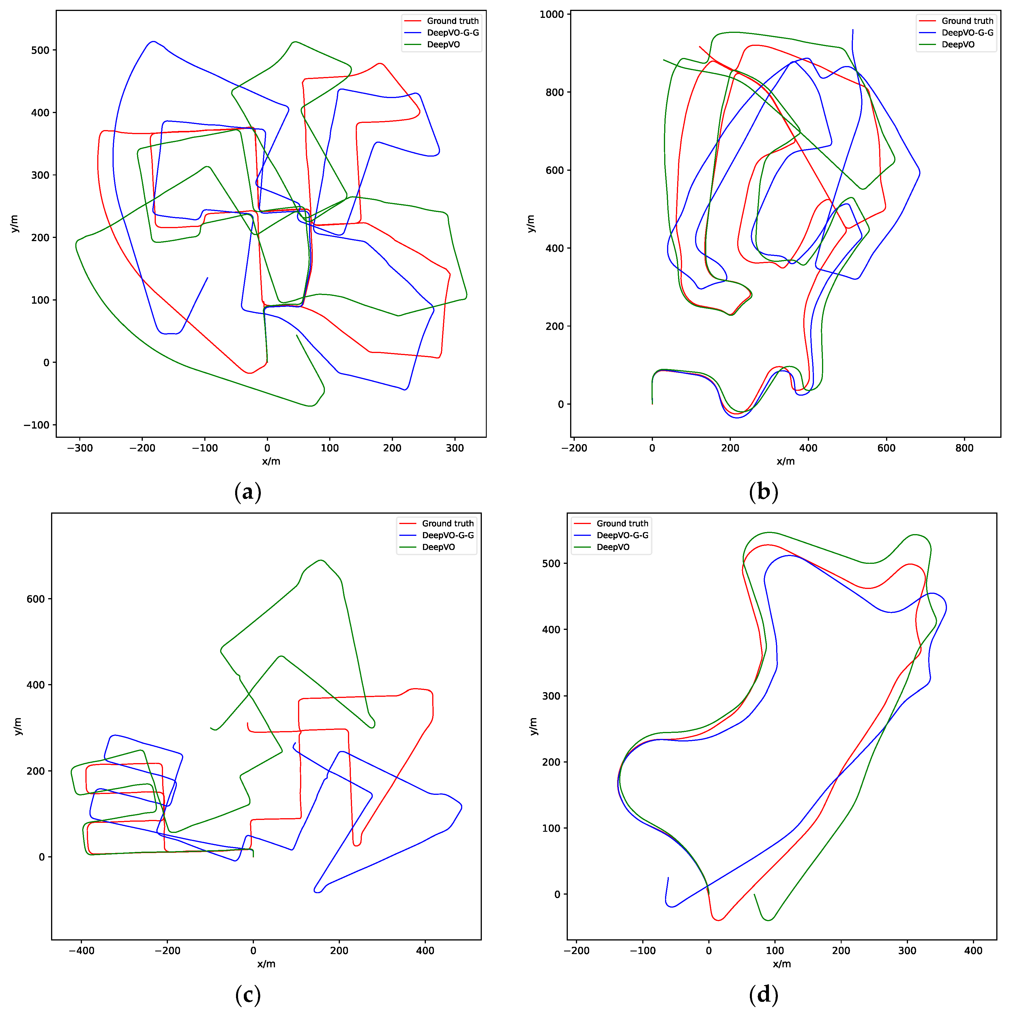
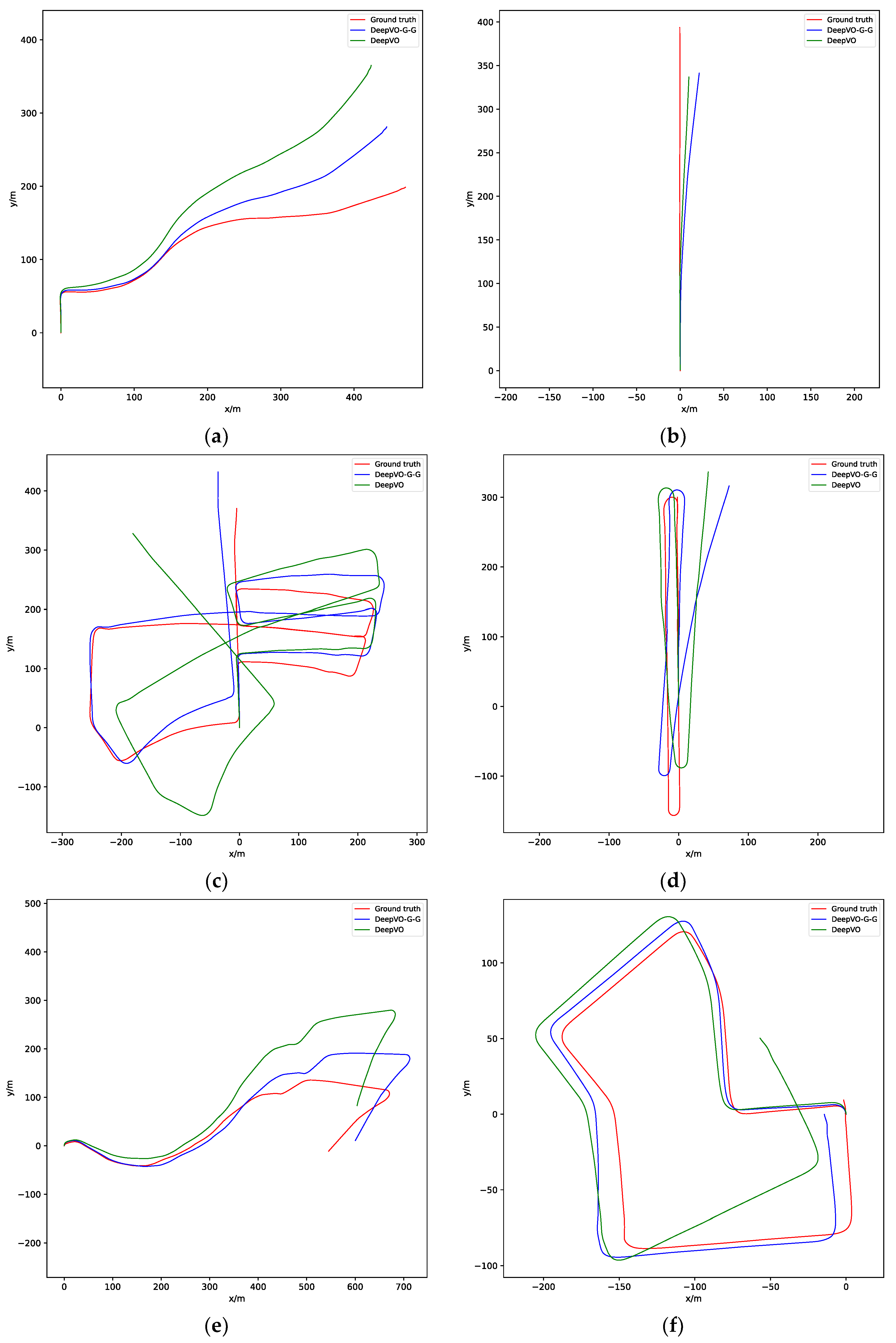
4.2. Experiment on Dataset with Ground Truth

Since the absolute scale is not feasible to obtain from the monocular visual odometry, the localization results were manually aligned with the ground truth. Therefore, the scales of monocular VISO2 (VISO2-M) and SC-Sfmlearner were aligned to the ground truth for a fair comparison. The DeepVO was implemented referring to [7]. The network was trained under the same settings as DeepVO-Graph and DeepVO-Graph-Geodesic (DeepVO-G-G) for a fair comparison since there is no official public code available. DeepVO-Graph indicates the rotation loss term is computed with the angle in Euclidean distance manner, while DeepVO-Graph-Geodesic represents the rotation loss term is computed with the proposed geodesic distance (new rotation loss). In the experiment, DeepVO, DeepVO-Graph, and Deep-Graph-Geodesic were trained with sequences 00, 02, 08, 09, and tested with sequences 03, 04, 05, 06, 07, 10, as in [7]. SC-Sfmlearner was trained with sequences from 00 to 08 and tested with sequences 09, 10 [48]. TrajNet was trained with sequences 00–06 and tested with 07–10 [49].
T e r r , R e r r , ATE, RPE(m), and RPE(°) metrics are widely used to evaluate the performance of VO/SLAM methods [7,9,48]. The KITTI Odometry criterion evaluates the possible sub-sequences of length (100, …, 700, 800) meters and reports the average translational error T e r r (%) and rotational errors R e r r (°/100 m). The relative pose error (RPE) measures frame-to-frame relative pose error. The absolute trajectory error (ATE) measures the root-mean-square error between the translation of predicted camera poses and ground truth. The RPE and ATE are computed as Equations (9)–(12).
E i = Q i 1 Q i + Δ 1 P i 1 P i + Δ
RMSE E 1 : n , Δ = 1 m i = 1 m trans E i 2 1 2
RPE = 1 n Δ = 1 m RMSE E 1 : n , Δ
F i = Q i 1 P i
ATE = 1 m i = 1 m trans F i 2 1 2
where P, Q  S E 3 , P and Q represent the predicted and the ground truth poses, respectively. Δ represents the time interval. trans E i can be replaced by rots E i . trans E i and rots E i represent the translation and the rotation parts of E i , respectively.
Table 2 and Table 3 show the quantitative results of training and testing sequences, respectively. The top two results are labeled in bold. It can be seen from the tables that both DeepVO-Graph and DeepVO-G-G are overall more accurate than DeepVO. The DeepVO-G-G and DeepVO-Graph exceed DeepVO and VISO2-M on the ATE index of sequences 00, 08 on the training dataset and maintain a competitive performance on most indexes on 02, 09 sequences. The DeepVO-G-G achieve the top two performance on sequences 03, 05, 07, 10 in terms of the ATE and better performance on the other sequences.
The SC-Sfmlearner has also achieved top two results on most of the sequences. However, the SC-Sfmlearner was trained using more sequences, i.e., sequences 02–08, and sequences 09, 10 were used for testing. The TrajNet was also trained with more sequences (00–06) than the proposed method. The proposed method shows comparable performances on common test sequences 07 and 10. Regarding test sequence 10, the DeepVO-G-G even achieves better performance, which also verifies the effectiveness of the proposed method. Both the DeepVO-Graph and DeepVO-G-G can boost the performance of DeepVO. The DeepVO-Graph shows better ATE results on long-distance sequences 05, 06, 07, 10 than the DeepVO. The DeepVO-G-G verifies that the geodesic distance can improve the performance compared with the Deep-Graph, especially for sequence 07. The results of DeepVO-G-G and DeepVO-Graph show that the graph-constrained loss functions can obtain a better performance to address the accumulated errors.
It should be noted that neither scale estimation nor post alignment to ground truth was conducted for DeepVO-Graph and DeepVO-G-G. The 2D trajectory comparison results are shown in Figure 4 and Figure 5. The X-axis and Y-axis represent the x and y coordinates of the absolute pose of images, respectively. For clarity, only the trajectories of DeepVO, DeepVO-G-G, and ground truth are plotted. The quantitative comparisons of various methods are shown in Table 2 and Table 3. The DeepVO-G-G consistently yields better performance for both translation and rotation compared with the DeepVO and others.
The performance of DeepVO-G-G is better than DeepVO-Graph on the test dataset. However, the DeepVO-G-G is not better than the DeepVO-Graph on the training dataset. This also proves that the proposed loss component has better generalization performance. The inference runtime of the proposed model on every test sequence is shown in Table 4. It can be observed that the inference speed is fast since it can be processed in parallel without additional steps.

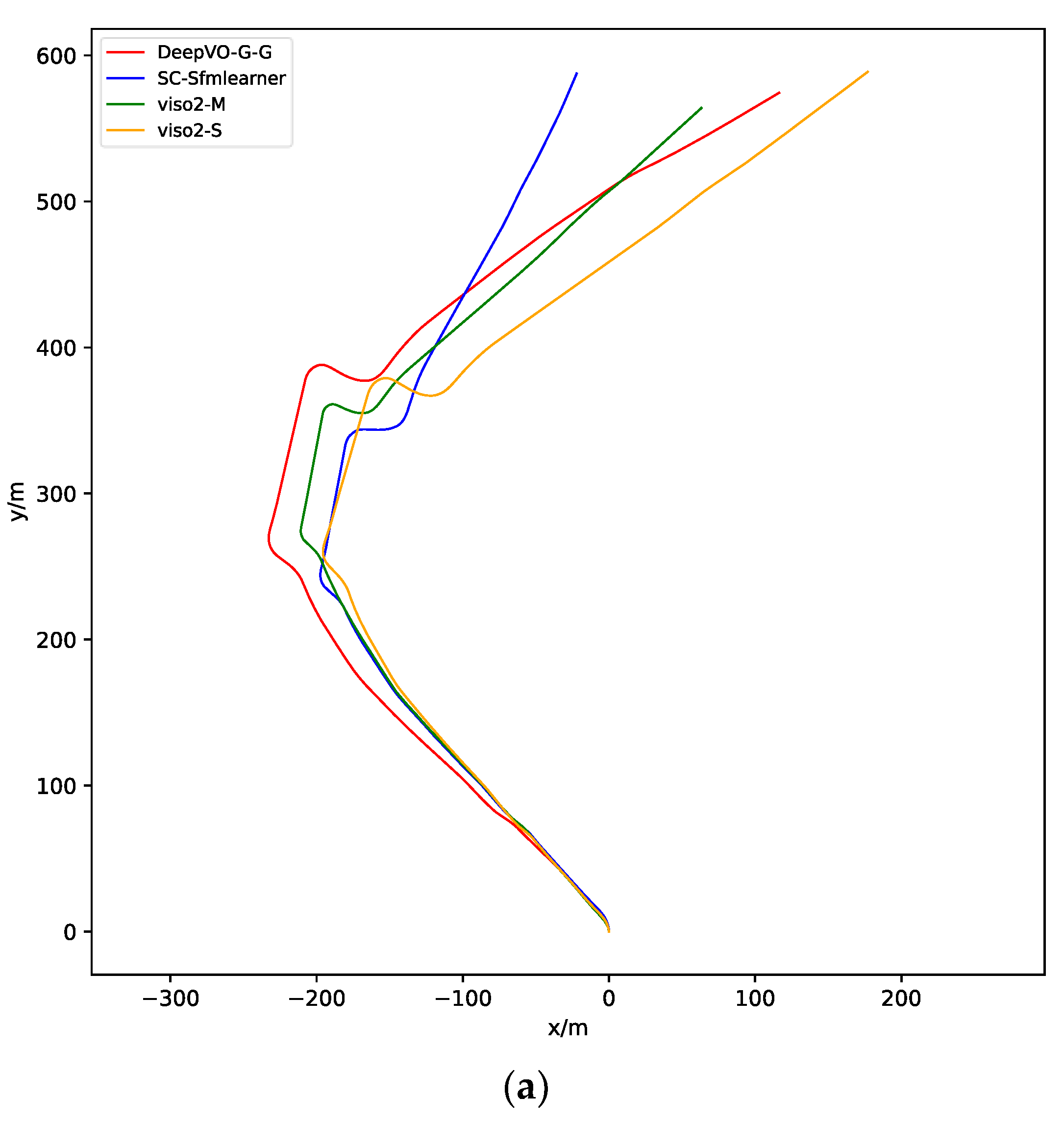
4.3. Experiment on Dataset without Ground Truth

To evaluate the performance of the proposed method, it was tested on test sequences 11, 15 using the former experiment model. Since no ground truth trajectory is provided, only the qualitative analysis is performed by generating the trajectory. The VISO2-S is chosen as the ground truth since its effectiveness has been accepted. The proposed method is also compared with SC-Sfmlearner, DeepVO-G-G, and VISO2-M.
The scale of VISO2-M and SC-Sfmlearner is obtained by aligning to the VISO2-S. The results are shown in Figure 6. The DeepVO-G-G and VISO2-M perform better in sequence 11; the SC-Sfmlearner is poorer than the others. Sequence 15 is more challenging (longer distances and scene complexity) than sequence 11. However, the proposed method is closer to the VISO2-S than VISO2-M and SC-Sfmlearner on sequence 15, which demonstrates that the proposed method achieves better performance than the traditional monocular visual odometry and other deep learning-based methods.

5. Discussion

5.1. Effect of Different Sliding Window Sizes

The sliding window size is a key parameter for graph loss. Theoretically, larger window size brings in complex graphs and stronger geometric constraints, which lead to better performance. However, it also demands larger computational resources. Therefore, due to the computing resource limitation, a balance has to be made between efficiency and accuracy.
To find the proper window size, three groups of windows lengths were set. The first group of window lengths were randomly selected between 5 and 10, the second group of window lengths ranged from 15–20, and the third group of window lengths ranged from 25–30. Sequences 00 and 08 were used to train the network, and sequences 09 and 10 were used for validation. The maximum iteration was 160 epochs. The rest of the parameters were set the same as previous experiments.
ATE, T e r r , R e r r are used to report the performance and the results are shown in Figure 7. The abscissa axes 0–5, 45–50, 75–80, and 115–120 represent that the best model among the intervals is selected for comparison to avoid accidental error factors. It can be seen from Figure 7 that the larger window size (length (25–30)) obtains the best performance with the lowest values in terms of ATE, T e r r , and R e r r when the model is fully trained. Another interesting fact is that the network converges more quickly with smaller window size than the larger window size since the window size 5–10 obtains better performance than the other two with fewer iterations.

5.2. Effect of Sequence Overlap

Given fixed window size, two sequences strategies are compared, i.e. with and without overlapping. Figure 8 shows the general idea of with and without the overlapping strategy. Table 5 and Table 6 show the performance of the model trained with and without overlap data augmentation strategy for training sequences (00,08) and test sequences (09,10), respectively. It can be seen that using the overlapping strategy can make the training more stable and improve the prediction accuracy.
Figure 9 shows that the model trained with the overlapping strategy of data augmentation tends to be smoother rather than oscillating both in the train and test dataset sequences.

6. Conclusions

In this paper, two novel losses based on graph and geodesic distance constraints are proposed for deep learning-based visual odometry, which exploits the relative pose constraints from image sequences. The experiments show that the graph loss outperforms the traditional loss designed based on the consecutive images. The graph loss not only considers the relative pose loss of consecutive images, but also the relative pose of non-consecutive images. The relative pose of non-consecutive images is not directly predicted but computed from the relative pose of the consecutive images. The geodesic rotation loss is constructed by the geodesic distance and the model regresses Lie algebra so(3) (3D vector). Lie algebra is introduced into the loss component of the deep learning-based poses estimation methods. Due to eliminating the self-constraint of the regression variable, the loss module can reduce the difficulty of training the poses regression. This allows a robust and stable convergence, and further improves the performance of deep learning-based visual odometry.
Comparative experiments are conducted on the KITTI odometry dataset. The KITTI odometry dataset contains different traffic scenes. The obtained results validate that the proposed method improves the important loss components in deep learning-based visual odometry methods. The proposed loss components can be easily integrated into other deep learning-based pose estimation tasks. The proposed method is also compared with the latest methods to verify its effectiveness. And the source code and weight can be found at https://github.com/fangxu622/Deep-Graph-VO (accessed on 1 March 2022).
Finally, the effects of different sliding window sizes are analyzed. The analysis shows that the large window size provides better performance, and a suitable sliding window size is obtained to achieve a balance between efficiency and accuracy. In order to explore the effect of overlapping strategies, two strategies are compared: with/without overlapping. It is found that sequence with overlapping shows better performance. In the future, the authors plan to fuse multiple sensors observation with Kalman filtering or factor graph optimization using deep learning techniques to improve the performance of learning-based visual odometry.

Author Contributions

Conceptualization, X.F. and Q.L. (Qing Li); methodology, X.F. and Q.L. (Qing Li); software, X.F. and K.D.; validation, Q.L. (Qing Li) and K.D.; writing—original draft preparation, X.F. and K.D.; writing—review and editing, X.F. and K.D.; visualization, Q.L. (Qing Li); supervision, Q.L. (Qingquan Li) and J.Z.; project administration, Q.L. (Qingquan Li) and J.Z.; funding acquisition, J.Z. All authors have read and agreed to the published version of the manuscript.

Funding

This work was supported in part by the Shenzhen Institute of Artificial Intelligence and Robotics for Society, in part by the Science and Research Service Project of Shenzhen Metro Group Co., Ltd. under Grant STJS-DT413-KY002/2021. This work was also supported in part by the China Postdoctoral Science Foundation (Grant No. 2021M702232). This work was also supported in part by the Basic and Applied Basic Research Funding Program of Guangdong Province of China (Grant No. 2019A1515110303).

Data Availability Statement

Data available in a publicly accessible repository that does not issue DOIs. Publicly available datasets were analyzed in this study. This data can be found here: http://www.cvlibs.net/datasets/kitti/eval_odometry.php (accessed on 1 March 2022).

Conflicts of Interest

The authors declare no conflict of interest.

References

  1. Scaramuzza, D.; Fraundorfer, F. Visual Odometry [Tutorial]. IEEE Robot. Autom. Mag. 2011, 18, 80–92. [Google Scholar] [CrossRef]
  2. Nister, D.; Naroditsky, O.; Bergen, J. Visual odometry. In Proceedings of the 2004 IEEE Computer Society Conference on Computer Vision and Pattern Recognition, CVPR 2004, Washington, DC, USA, 27 June–2 July 2004; Volume 1, pp. 652–659. [Google Scholar] [CrossRef]
  3. Weiss, S.; Scaramuzza, D.; Siegwart, R. Monocular-SLAM–based navigation for autonomous micro helicopters in GPS-denied environments. J. Field Robot. 2011, 28, 854–874. [Google Scholar] [CrossRef]
  4. Kröse, B.J.; Vlassis, N.; Bunschoten, R.; Motomura, Y. A probabilistic model for appearance-based robot localization. Image Vis. Comput. 2001, 19, 381–391. [Google Scholar] [CrossRef]
  5. Wolf, J.; Burgard, W.; Burkhardt, H. Robust vision-based localization by combining an image-retrieval system with Monte Carlo localization. IEEE Trans. Robot. 2005, 21, 208–216. [Google Scholar] [CrossRef]
  6. Wiseman, Y. Ancillary ultrasonic rangefinder for autonomous vehicles. Int. J. Secur. Its Appl. 2018, 12, 49–58. [Google Scholar] [CrossRef]
  7. Wang, S.; Clark, R.; Wen, H.; Trigoni, N. DeepVO: Towards End-to-End Visual Odometry with Deep Recurrent Convolutional Neural Networks. In Proceedings of the 2017 IEEE International Conference on Robotics and Automation (ICRA), Singapore, 29 May–3 June 2017; pp. 2043–2050. [Google Scholar] [CrossRef] [Green Version]
  8. Saputra, M.R.U.; de Gusmao, P.P.; Wang, S.; Markham, A.; Trigoni, N. Learning monocular visual odometry through geometry-aware curriculum learning. In Proceedings of the 2019 International Conference on Robotics and Automation (ICRA), Montreal, QC, Canada, 20–24 May 2019; pp. 3549–3555. [Google Scholar]
  9. Zhan, H.; Weerasekera, C.S.; Bian, J.-W.; Reid, I. Visual odometry revisited: What should be learnt? In Proceedings of the 2020 IEEE International Conference on Robotics and Automation (ICRA), Paris, France, 31 May–31 August 2020; pp. 4203–4210. [Google Scholar]
  10. Clark, R.; Wang, S.; Markham, A.; Trigoni, N.; Wen, H. Vidloc: A deep spatio-temporal model for 6-dof video-clip relocalization. In Proceedings of the IEEE Conference on Computer Vision and Pattern Recognition, Honolulu, HI, USA, 21–26 July 2017; pp. 6856–6864. [Google Scholar]
  11. Li, Q.; Zhu, J.; Cao, R.; Sun, K.; Garibaldi, J.M.; Li, Q.; Liu, B.; Qiu, G. Relative Geometry-Aware Siamese Neural Network for 6DOF Camera Relocalization. Neurocomputing 2021, 426, 134–146. [Google Scholar] [CrossRef]
  12. Xue, F.; Wu, X.; Cai, S.; Wang, J. Learning Multi-View Camera Relocalization With Graph Neural Networks. In Proceedings of the 2020 IEEE/CVF Conference on Computer Vision and Pattern Recognition (CVPR), Seattle, WA, USA, 13–19 June 2020; pp. 11372–11381. [Google Scholar] [CrossRef]
  13. Hochreiter, S.; Schmidhuber, J. Long short-term memory. Neural Comput. 1997, 9, 1735–1780. [Google Scholar] [CrossRef]
  14. Zhang, Z. A flexible new technique for camera calibration. IEEE Trans. Pattern Anal. Mach. Intell. 2000, 22, 1330–1334. [Google Scholar] [CrossRef] [Green Version]
  15. Kumar, G.; Bhatia, P.K. A detailed review of feature extraction in image processing systems. In Proceedings of the 2014 Fourth International Conference on Advanced Computing & Communication Technologies, Rohtak, India, 8–9 February 2014; pp. 5–12. [Google Scholar]
  16. Kummerle, R.; Grisetti, G.; Strasdat, H.; Konolige, K.; Burgard, W. G2O: A general framework for graph optimization. In Proceedings of the 2011 IEEE International Conference on Robotics and Automation, Shanghai, China, 9–13 May 2011; pp. 3607–3613. [Google Scholar] [CrossRef]
  17. Dellaert, F.; Kaess, M. Factor Graphs for Robot Perception. Found. Trends Robot. 2017, 6, 1–139. [Google Scholar] [CrossRef]
  18. Jiang, S.; Jiang, C.; Jiang, W. Efficient structure from motion for large-scale UAV images: A review and a comparison of SfM tools. ISPRS J. Photogramm. Remote Sens. 2020, 167, 230–251. [Google Scholar] [CrossRef]
  19. Ji, S.; Qin, Z.; Shan, J.; Lu, M. Panoramic SLAM from a multiple fisheye camera rig. ISPRS J. Photogramm. Remote Sens. 2020, 159, 169–183. [Google Scholar] [CrossRef]
  20. Qin, T.; Li, P.; Shen, S. VINS-Mono: A Robust and Versatile Monocular Visual-Inertial State Estimator. IEEE Trans. Robot. 2018, 34, 1004–1020. [Google Scholar] [CrossRef] [Green Version]
  21. Campos, C.; Elvira, R.; Rodriguez, J.J.G.; Montiel, J.M.M.; Tardos, J.D. ORB-SLAM3: An Accurate Open-Source Library for Visual, Visual–Inertial, and Multimap SLAM. IEEE Trans. Robot. 2021, 37, 1874–1890. [Google Scholar] [CrossRef]
  22. Rosinol, A.; Abate, M.; Chang, Y.; Carlone, L. Kimera: An open-source library for real-time metric-semantic localization and mapping. In Proceedings of the 2020 IEEE International Conference on Robotics and Automation (ICRA), Paris, France, 31 May–31 August 2020; pp. 1689–1696. [Google Scholar]
  23. Zhang, G. Towards Optimal 3D Reconstruction and Semantic Mapping. Ph.D. Thesis, University of California, Merced, CA, USA, 2021. [Google Scholar]
  24. Rosten, E.; Drummond, T. Machine learning for high-speed corner detection. In Proceedings of the European Conference on Computer Vision, Graz, Austria, 7–13 May 2006; Springer: Berlin/Heidelberg, Germany, 2006; pp. 430–443. [Google Scholar]
  25. Bay, H.; Ess, A.; Tuytelaars, T.; van Gool, L. Speeded-up robust features (SURF). Comput. Vis. Image Underst. 2008, 110, 346–359. [Google Scholar] [CrossRef]
  26. Calonder, M.; Lepetit, V.; Strecha, C.; Fua, P. Brief: Binary robust independent elementary features. In Proceedings of the European Conference on Computer Vision, Heraklion, Greece, 5–11 September 2010; Springer: Berlin/Heidelberg, Germany, 2010; pp. 778–792. [Google Scholar]
  27. Harris, C.; Stephens, M. A combined corner and edge detector. Alvey Vis. Conf. 1988, 15, 10–5244. [Google Scholar]
  28. Aguiar, A.; Sousa, A.; Santos, F.N.d.; Oliveira, M. Monocular Visual Odometry Benchmarking and Turn Performance Optimization. In Proceedings of the 2019 IEEE International Conference on Autonomous Robot Systems and Competitions (ICARSC), Porto, Portugal, 24–26 April 2019; pp. 1–6. [Google Scholar] [CrossRef]
  29. Geiger, A.; Ziegler, J.; Stiller, C. StereoScan: Dense 3d reconstruction in real-time. In Proceedings of the 2011 IEEE Intelligent Vehicles Symposium (IV), Baden-Baden, Germany, 5–9 June 2011; pp. 963–968. [Google Scholar] [CrossRef]
  30. Mur-Artal, R.; Tardós, J.D. ORB-SLAM2: An Open-Source SLAM System for Monocular, Stereo, and RGB-D Cameras. IEEE Trans. Robot. 2017, 33, 1255–1262. [Google Scholar] [CrossRef] [Green Version]
  31. Engel, J.; Schöps, T.; Cremers, D. LSD-SLAM: Large-Scale Direct Monocular SLAM. In Proceedings of the Computer Vision—ECCV 2014; Fleet, D., Pajdla, T., Schiele, B., Tuytelaars, T., Eds.; Springer International Publishing: Cham, Switzerland, 2014; Volume 8690, pp. 834–849. [Google Scholar] [CrossRef] [Green Version]
  32. Engel, J.; Koltun, V.; Cremers, D. Direct sparse odometry. IEEE Trans. Pattern Anal. Mach. Intell. 2017, 40, 611–625. [Google Scholar] [CrossRef]
  33. Krizhevsky, A.; Sutskever, I.; Hinton, G.E. Imagenet classification with deep convolutional neural networks. Commun. ACM 2017, 60, 84–90. [Google Scholar] [CrossRef]
  34. Redmon, J.; Farhadi, A. YOLOv3: An Incremental Improvement. arXiv 2018, arXiv:1804.02767. Available online: http://arxiv.org/abs/1804.02767 (accessed on 21 April 2021).
  35. Ren, S.; He, K.; Girshick, R.; Sun, J. Faster R-CNN: Towar ds Real-Time Object Detection with Region Proposal Networks. arXiv 2016, arXiv:1506.01497. Available online: http://arxiv.org/abs/1506.01497 (accessed on 19 February 2021). [CrossRef] [Green Version]
  36. Kwon, H.; Kim, Y. BlindNet backdoor: Attack on deep neural network using blind watermark. Multimed. Tools Appl. 2022, 81, 6217–6234. [Google Scholar] [CrossRef]
  37. Kendall, A.; Cipolla, R. Geometric Loss Functions for Camera Pose Regression With Deep Learning. In Proceedings of the IEEE Conference on Computer Vision and Pattern Recognition, Honolulu, HI, USA, 21–26 July 2017. [Google Scholar]
  38. Konda, K.R.; Memisevic, R. Learning visual odometry with a convolutional network. In Proceedings of the VISAPP (1), Berlin, Germany, 11–14 March 2015; pp. 486–490. [Google Scholar]
  39. Vu, T.; van Nguyen, C.; Pham, T.X.; Luu, T.M.; Yoo, C.D. Fast and efficient image quality enhancement via desubpixel convolutional neural networks. In Proceedings of the European Conference on Computer Vision (ECCV) Workshops, Munich, Germany, 8–14 September 2018. [Google Scholar]
  40. Jeon, M.; Jeong, Y.-S. Compact and Accurate Scene Text Detector. Appl. Sci. 2020, 10, 2096. [Google Scholar] [CrossRef] [Green Version]
  41. Kendall, A.; Grimes, M.; Cipolla, R. PoseNet: A Convolutional Network for Real-Time 6-DOF Camera Relocalization. In Proceedings of the 2015 IEEE International Conference on Computer Vision (ICCV), Santiago, Chile, 7–13 December 2015; pp. 2938–2946. [Google Scholar] [CrossRef] [Green Version]
  42. Zhou, L.; Luo, Z.; Shen, T.; Zhang, J.; Zhen, M.; Yao, Y.; Fang, T.; Quan, L. KFNet: Learning Temporal Camera Relocalization using Kalman Filtering. In Proceedings of the IEEE/CVF Conference on Computer Vision and Pattern Recognition, Seattle, WA, USA, 13–19 June 2020; pp. 4919–4928. [Google Scholar]
  43. Li, Q.; Zhu, J.; Liu, J.; Cao, R.; Fu, H.; Garibaldi, J.M.; Li, Q.; Lin, B.; Qiu, G. 3D map-guided single indoor image localization refinement. ISPRS J. Photogramm. Remote Sens. 2020, 161, 13–26. [Google Scholar] [CrossRef]
  44. Costante, G.; Mancini, M.; Valigi, P.; Ciarfuglia, T.A. Exploring Representation Learning With CNNs for Frame-to-Frame Ego-Motion Estimation. IEEE Robot. Autom. Lett. 2016, 1, 18–25. [Google Scholar] [CrossRef]
  45. Muller, P.; Savakis, A. Flowdometry: An optical flow and deep learning based approach to visual odometry. In Proceedings of the 2017 IEEE Winter Conference on Applications of Computer Vision (WACV), Santa Rosa, CA, USA, 24–31 March 2017; pp. 624–631. [Google Scholar]
  46. Dosovitskiy, A.; Fischer, P.; Ilg, E.; Hausser, P.; Hazirbas, C.; Golkov, V.; Van Der Smagt, P.; Cremers, D.; Brox, T. Flownet: Learning optical flow with convolutional networks. In Proceedings of the IEEE International Conference on Computer Vision, Santiago, Chile, 7–13 December 2015; pp. 2758–2766. [Google Scholar]
  47. Wang, S.; Clark, R.; Wen, H.; Trigoni, N. End-to-end, sequence-to-sequence probabilistic visual odometry through deep neural networks. Int. J. Robot. Res. 2018, 37, 513–542. [Google Scholar] [CrossRef]
  48. Bian, J.; Li, Z.; Wang, N.; Zhan, H.; Shen, C.; Cheng, M.M.; Reid, I. Unsupervised scale-consistent depth and ego-motion learning from monocular video. Adv. Neural Inf. Process. Syst. 2019, 32, 35–45. [Google Scholar]
  49. Zhao, C.; Tang, Y.; Sun, Q.; Vasilakos, A.V. Deep Direct Visual Odometry. IEEE Trans. Intell. Transp. Syst. 2021, 1–10. [Google Scholar] [CrossRef]
  50. Clark, R.; Wang, S.; Wen, H.; Markham, A.; Trigoni, N. VINet: Visual-Inertial Odometry as a Sequence-to-Sequence Learning Problem. arXiv 2017, arXiv:1701.08376. [Google Scholar]
  51. Liu, Q.; Li, R.; Hu, H.; Gu, D. Using Unsupervised Deep Learning Technique for Monocular Visual Odometry. IEEE Access 2019, 7, 18076–18088. [Google Scholar] [CrossRef]
  52. Jiao, J.; Jiao, J.; Mo, Y.; Liu, W.; Deng, Z. Magicvo: End-to-end monocular visual odometry through deep bi-directional recurrent convolutional neural network. arXiv 2018, arXiv:1811.10964. [Google Scholar]
  53. Fang, Q.; Hu, T. Euler angles based loss function for camera relocalization with Deep learning. In Proceedings of the 2018 IEEE 8th Annual International Conference on CYBER Technology in Automation, Control, and Intelligent Systems (CYBER), Tianjin, China, 19–23 July 2018. [Google Scholar]
  54. Li, D.; Dunson, D.B. Geodesic Distance Estimation with Spherelets. arXiv 2020, arXiv:1907.00296. Available online: http://arxiv.org/abs/1907.00296 (accessed on 28 January 2022).
Figure 1. (a) Traditional loss computed from consecutive nodes; (b) the proposed graph loss is computed from a constructed graph that not only considers the constraints between the consecutive images, but also between the non-consecutive images (red edges).
Remotesensing 14 01854 g001
Figure 2. The network architecture of deep learning-based visual odometry.
Remotesensing 14 01854 g002
Figure 3. Computation of graph loss.
Remotesensing 14 01854 g003
Figure 4. The trajectories of the proposed method on the training sequences. (a) Sequence 00; (b) Sequence 02; (c) Sequence 08; (d) Sequence 09.
Remotesensing 14 01854 g004
Figure 5. The trajectories of the proposed method on the test sequences. (a) Sequence 03; (b) Sequence 04; (c) Sequence 05; (d) Sequence 06; (e) Sequence 07; (f) Sequence 10.
Remotesensing 14 01854 g005
Figure 6. The trajectories of sequences 11 and 15. (a) Sequence 11; (b) Sequence 15.
Remotesensing 14 01854 g006aRemotesensing 14 01854 g006b
Figure 7. Analysis of effects on different sliding window sizes. (a) ATE; (b) T e r r ; (c) R e r r .
Remotesensing 14 01854 g007
Figure 8. Demonstration of sequence overlap.
Remotesensing 14 01854 g008
Figure 9. Comparison of sequence overlap and no overlap trajectories. (a) Sequence 00; (b) Sequence 08; (c) Sequence 09; (d) Sequence 10.
Remotesensing 14 01854 g009
Table 1. The parameters of deep learning-based visual odometry model.
LayerOutput SizeKernel SizePaddingStrideChannelDropout
Input size6 × 608 × 184 (image pairs)
Conv1(304,92)7 × 732640.0
Conv2(152,46)5 × 5221280.0
Conv3(76,23)5 × 5222560.0
Conv3_1(76,23)3 × 3112560.1
Conv4(38,12)3 × 3125120.1
Conv4_1(38,12)3 × 3125120.1
Conv5(19,6)3 × 3115120.1
Conv5_1(19,6)3 × 3125120.3
Conv6 (10,3)3 × 31110240.2
LSTMnum_layer = 2, input_size = 30,720 (1024 × 3 × 10), hidden_size = 1024
FC layer1Input_feature = 1024, output_feature = 128
FC layer2Input_size = 128, output_size = 6
Table 2. Comparison of various visual odometry methods on the training dataset. (Bold denotes best performance, underline denotes second best performance).
SequenceVISO2-M [29]SC-Sfmlearner [48]DeepVO [7]DeepVO-Graph (Ours)DeepVO-G-G (Ours)
00 T e r r 37.149.884.12.993.35
R e r r 15.843.911.761.371.43
ATE142.14137.3483.7731.873.02
RPE(m)0.3770.0930.0230.0180.029
RPE(°)1.1610.1340.2090.1050.198
02 T e r r 6.387.275.863.863.98
R e r r 1.392.191.751.341.37
ATE86.73199.2795.0586.98147.13
RPE(m)0.1190.0810.0290.0230.034
RPE(°)0.1830.0890.1730.0930.163
08 T e r r 24.4618.265.592.653.38
R e r r 8.032.012.261.081.54
ATE132.79133.79180.9128.09128.09
RPE(m)0.3120.2440.0260.0190.030
RPE(°)0.8960.070.1640.0860.156
09 T e r r 4.4111.244.324.043.36
R e r r 1.233.341.521.491.29
ATE18.03121.9643.7137.8938.83
RPE(m)0.1210.1060.0250.0220.031
RPE(°)0.1210.1060.1420.080.137
Table 3. Comparison of various visual odometry methods on the test dataset (Note: SC-Sfmlearner train sequences: 00–08, test sequences 09,10. Their results are used only for references. DeepVO, DeepVO-Graph, DeepVO-G-G are the same experiment settings. Bold denotes best performance, underline denotes second best performance).
SequenceVISO2-M [29]SC-Sfmlearner [48]TrajNet [49]DeepVO [7]DeepVO-Graph (Ours)DeepVO-G-G (Ours)
03 T e r r 16.884.45-15.069.7210.00
R e r r 5.212.77-6.64.54.87
ATE91.9215.67-87.246.5741.92
RPE(m)0.1010.055-0.0650.0620.058
RPE(°)0.4230.062-0.1620.1090.153
04 T e r r 1.733.28-8.048.977.11
R e r r 1.390.95-2.461.912.60
ATE7.627.15-16.0317.3215.55
RPE(m)0.1060.069-0.1260.1390.111
RPE(°)0.0980.049-0.110.0880.117
05 T e r r 16.86.02-7.87.766.55
R e r r 5.141.8-2.653.02.59
ATE108.0255.91-83.5155.136.03
RPE(m)0.2960.069-0.0810.0830.073
RPE(°)0.290.063-0.1580.1060.153
06 T e r r 4.5710.73-9.999.438.43
R e r r 1.452.18-1.961.92.36
ATE33.8144.5-43.1242.7739.84
RPE(m)0.090.135-0.1250.1260.107
RPE(°)0.1190.167-0.1340.0910.134
07 T e r r 26.157.1310.936.979.014.87
R e r r 15.112.385.154.796.782.82
ATE48.2522.41-30.2539.3213.99
RPE(m)0.3590.056-0.0630.060.055
RPE(°)0.9280.068-0.160.1290.168
10RPE(°)31.9910.0711.914.1714.0210.91
R e r r 9.064.912.844.294.23.50
ATE229.1978.28-126.4597.364.08
RPE(m)0.4860.103-0.1220.1210.111
RPE(°)0.8240.113-0.2050.1470.198
Table 4. The inference runtime of the proposed model for different sequences (experiment environment: Ubuntu 18.04, PyTorch Library, Intel Xeon Gold 5222 CPU, RAM 64G, NVIDIA Titan RTX GPU 24G).
SequenceNumber of FramesInference Runtime (s)
038014.6
042713.6
0527617.7
0611014.2
0711014.2
1012014.3
Table 5. Comparison of overlap and no-overlap on train sequences.
0008
T e r r R e r r ATERPE(m)RPE(°) T e r r R e r r ATERPE(m)RPE(°)
Overlap2.911.3456.330.0170.2104.21.84149.320.0170.166
No-overlap9.514.37241.770.0200.2159.744.21321.380.0200.171
Table 6. Comparison of overlap and no-overlap on test sequences.
0910
T e r r R e r r ATERPE(m)RPE(°) T e r r R e r r ATERPE(m)RPE(°)
Overlap13.774.47111.20.150.21513.35.8280.640.1290.267
No-overlap15.585.49208.560.1380.20123.039.57266.300.1210.244
Publisher’s Note: MDPI stays neutral with regard to jurisdictional claims in published maps and institutional affiliations.

