Performance and the Optimal Integration of Sentinel-1/2 Time-Series Features for Crop Classification in Northern Mongolia

Abstract

Accurate and early crop-type maps are essential for agricultural policy development and food production assessment at regional and national levels. This study aims to produce a crop-type map with acceptable accuracy and spatial resolution in northern Mongolia by optimizing the combination of Sentinel-1 (S1) and Sentinel-2 (S2) images with the Google Earth Engine (GEE) environment. A total of three satellite data combination scenarios are set, including S1 alone, S2 alone, and the combination of S1 and S2. In order to avoid the impact of data gaps caused by clouds on crop classification, this study reconstructed the time series of S1 and S2 with a 10-day interval using the median composite method, linear moving interpolation, and Savitzky–Golay (SG) filter. Our results indicated that crop-type classification accuracy increased with the increase in data length to all three data combination scenarios. S2 alone has higher accuracy than S1 alone and the combination of S1 and S2. The crop-type map with the highest accuracy was generated using S2 data from 150 days of the year (DOY) (11 May) to 260 DOY (18 September). The OA and kappa were 0.93 and 0.78, respectively, and the F1-score for spring wheat and rapeseed were 0.96 and 0.80, respectively. The classification accuracy of the crop increased rapidly from 210 DOY (end of July) to 260 DOY (August to mid-September), and then it remained stable after 260 DOY. Based on our analysis, we filled the gap of the crop-type map with 10 m spatial resolution in northern Mongolia, revealing the best satellite combination and the best period for crop-type classification, which can benefit the achievement of sustainable development goals 2 (SDGs2).

1. Introduction

Agriculture is a vital sector in the economy of Mongolia, which accounted for 10.8% of the Gross Domestic Product (GDP) in 2018 [1]. The northern part of Mongolia is a agriculturally dominated region, and is vulnerable to weather conditions since about 80% of the cultivated land is rain-fed. As the principal cereal crop of Mongolia, wheat production has drastically declined due to policy changes, investment reduction, and successive severe droughts since the mid-1990s [2]. The accurate and timely mapping of crop types is essential for estimating food production and agricultural field management [3] to achieve food security and other related Sustainable Development Goals [4,5]. Previous studies in Mongolia focused on monitoring desertification and land degradation [6,7], wheat yield estimation [8], cropland suitability [9,10], soil moisture content [11,12], drought monitoring [13,14], and land cover classification [15,16]. However, a crop-type map with a high spatial resolution has never been constructed in Mongolia due to data and computation constraints. It is, therefore, desirable to design an effective way to fill the gap in crop-type maps in Mongolia.

Remote-sensing-based techniques are effective and reliable for crop-type mapping and land cover classification [17,18,19]. In this regard, many methods have been proposed for crop-type classification using several pixel-based machine-learning classification algorithms such as random forest [20], support vector machine [3], and artificial neural network [21]. New satellite images with high spatial resolution and visiting frequency, such as Sentinel and Landsat imagery, provide an opportunity for large-scale crop mappings. Geospatial cloud-computing platforms offer a good solution for data processing of large areas, for instance, Google Earth Engine (GEE) [22], coupling plentiful satellite sources and strong computing ability. Nowadays, GEE is widely used in geospatial analysis, landcover mapping, and crop identification, such as landcover mapping [23], vegetation greenness analysis [24], land degradation [25,26], and mapping of paddy [27,28], maize [29] and wheat [30]. New satellite and state-of-the-art cloud computing has significantly accelerated the development of crop identification and crop-type mapping for different spatial scales, such as 10 m crop type mapping in northeast China [31], national crop-type mapping in Beligum [32], paddy mapping in northeast Asia [33], and continental crop-type mapping in the European Union [34]. Some automatic crop-type mapping systems were developed for national-scale crop-type mapping, such as the Sen2Agri system [35].

Successful crop-type classification depends on selecting suitable satellite imagery and feature exploration. Optimal satellite imagery plays a critical role in crop classification, such as in crop-type mapping in northeast China [31]. However, one of the main difficulties with optical data is its acquisition in cloudy conditions, which leads to missing or severely distorted values [36,37]. A variety of methods have been developed to reconstruct the time series of features for crop-type classification, such as median composites [38], percentile composites [27], linear moving interplolation [38], SG filter [39], and a combination of mixed temporal reconstruction [31,40]. In addition, synthetic aperture radar (SAR) data are a promising option to address this challenge, as cloud occlusion has little effect on radar backscattering [41]. Therefore, exploring the backscattering coefficient features in a different growing stage is an alternative for other crops. For instance, several studies have utilized Sentinel-1 for crop classification to overcome S2 limitations [42,43,44,45,46,47]. Several studies demonstrate that using S1 and S2 images as an input can achieve a high accuracy [32,48,49]. Therefore, it is necessary to compare the performance difference using different data combination strategies. The availability of both S1 and S2 in the GEE environment gives us an excellent opportunity to use these three combinations to pick up the best classification result for our study area.

Determining the most suitable temporal windows for early crop determination is critical for timely agricultural policymaking. The longer the time series of data used for classification, the higher the crop classification accuracy as the information becomes rich. Therefore, comparing the accuracy (e.g., overall accuracy (OA) or F1-score) change with time to find the time point with the acceptable or highest accuracy is the typical approach for temporal windows’ confirmation and earlier crop-type classification. For example, You et al. [40] identified the earliest identifiable timing of rice, corn, and soybean in Heilongjiang province, China, through model transfer and equal temporal intervals’ data integration. Hu et al. found that April to August is the best time window to identify crop types in China’s Hetao irrigation district [50]. Thomas et al. [51] identified the best discrimination period for rice, maize, and sorghum in southeast Australia. Crop classification with accepted accuracy can be achieved five months before the end of the season in northern Italy [52]. Timely and early crop-type identification is also critical for Mongolia’s crop production. Therefore, it is necessary to determine the most suitable time windows for crop type classification in Mongolia.

This study takes northern Mongolia as the study area. This study aims to design a crop classification framework and fill the crop-type map gap with acceptable spatial resolution. In addition, this research expects to answer the following scientific questions:

(1)

Which satellite combination is best for crop-type classification in northern Mongolia?

(2)

What are the suitable time windows for crop classification in northern Mongolia?

(3)

What is the most effective and sensitive metric for crop classification?

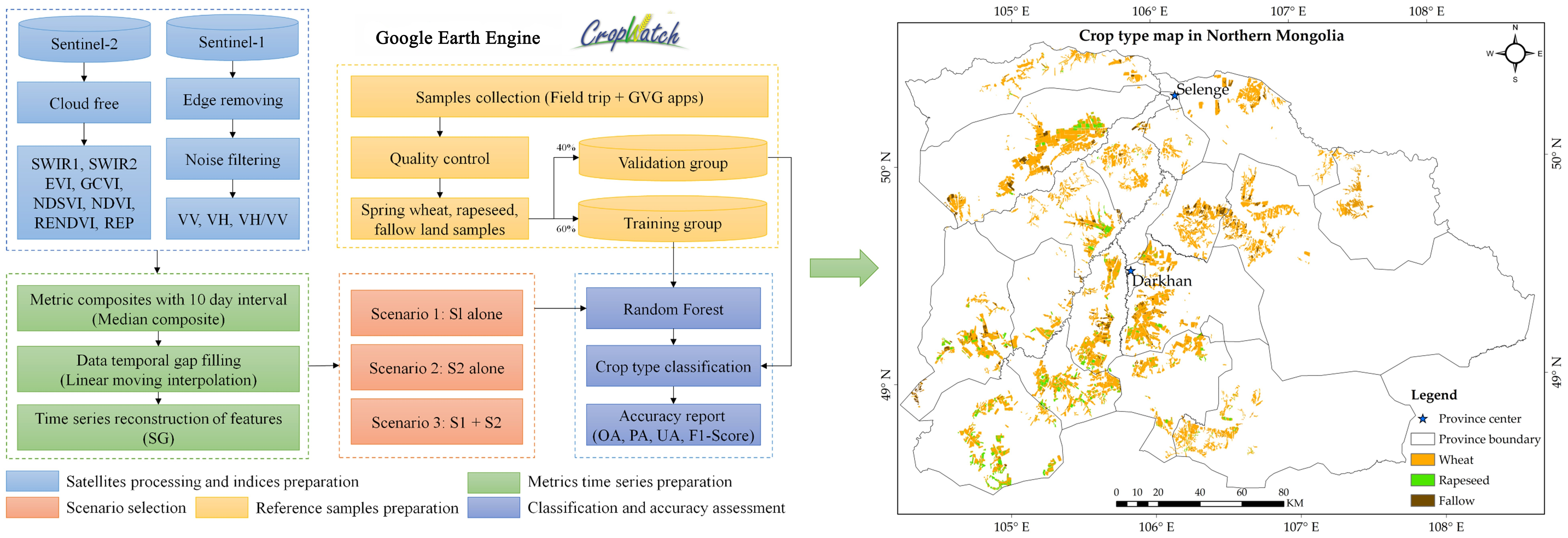
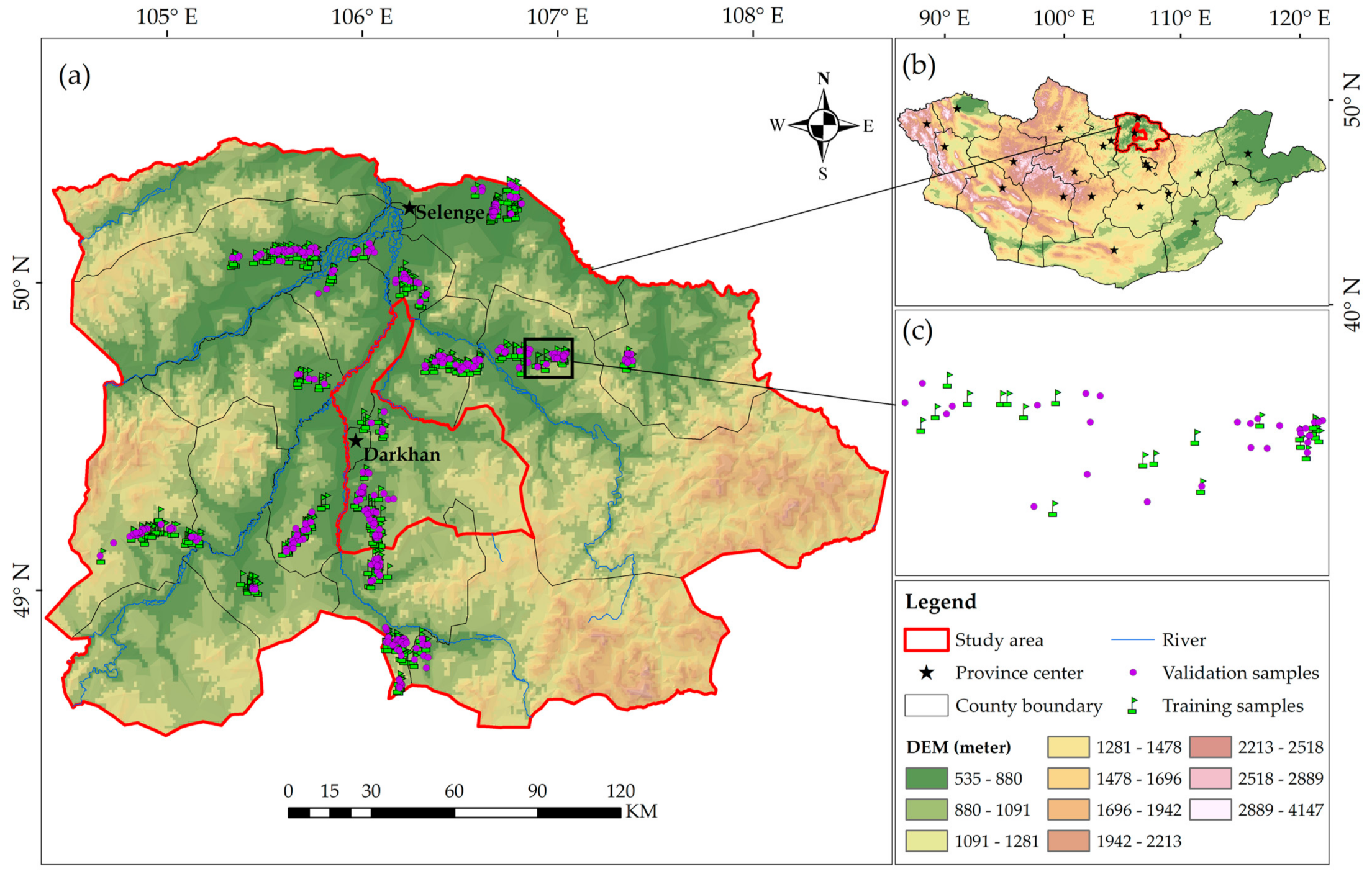
2. Study Area and Data

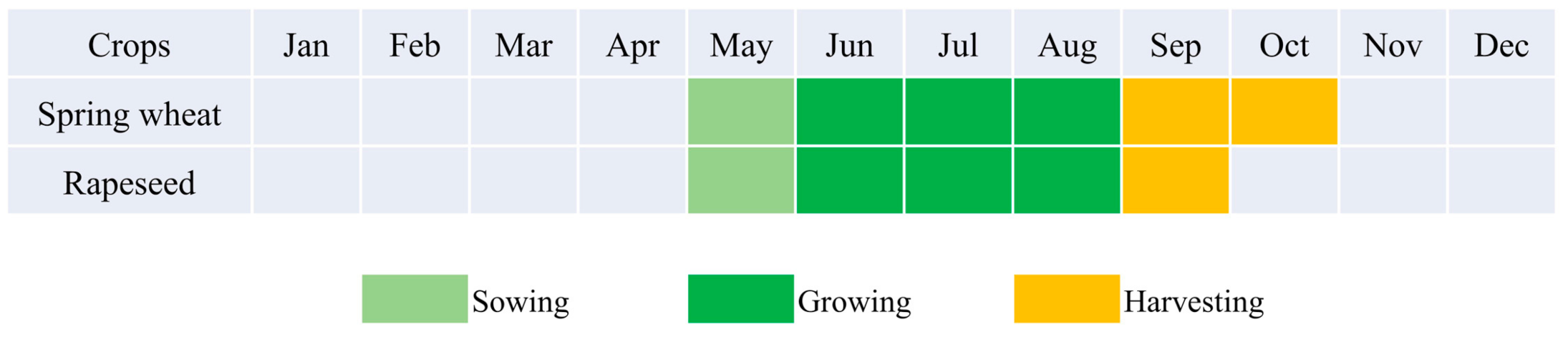
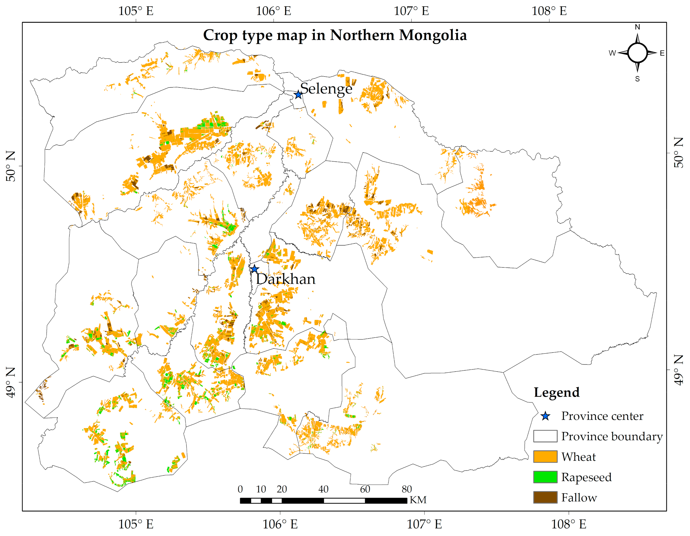
2.1. Study Area

The provinces of Darkhan and Selenge are located in the north-central part of Mongolia (Figure 1). The study area has the most favorable natural conditions for crop growth and produced approximately 42% of Mongolia’s national wheat in 2018 [1]. Almost all crops in the study area are rainfed crops, which are very sensitive to changes in weather conditions.

The study area is dominated by a temperate continental climate with a dry and cold winter and a humid and warm summer. According to meteorological data obtained from the Information and Research Institute of Meteorology, Hydrology, and Environment (IRIMHE) in Mongolia, annual precipitation in 2018 was 313 mm, with approximately 71% (224 mm) of the annual precipitation occurring in June–August. The average annual temperature is 2 °C, being −22.5 °C in January and 20 °C in July (Figure 2). Due to the constraints of the accumulated temperature, crops in the area are dominated by cold-tolerant and early maturing spring wheat varieties and rapeseed.

Spring wheat and rapeseed are the major crops of the study area. Figure 3 shows the phenology of spring wheat and rapeseed. In general, spring wheat is sown in early May, the critical growing period is from June to August, and the harvest period is from late September to early October. Rapeseed has similar phenology to spring wheat, which is sown in May and harvested in September. The length of the growing period of crops in the region is 90 to 140 days.

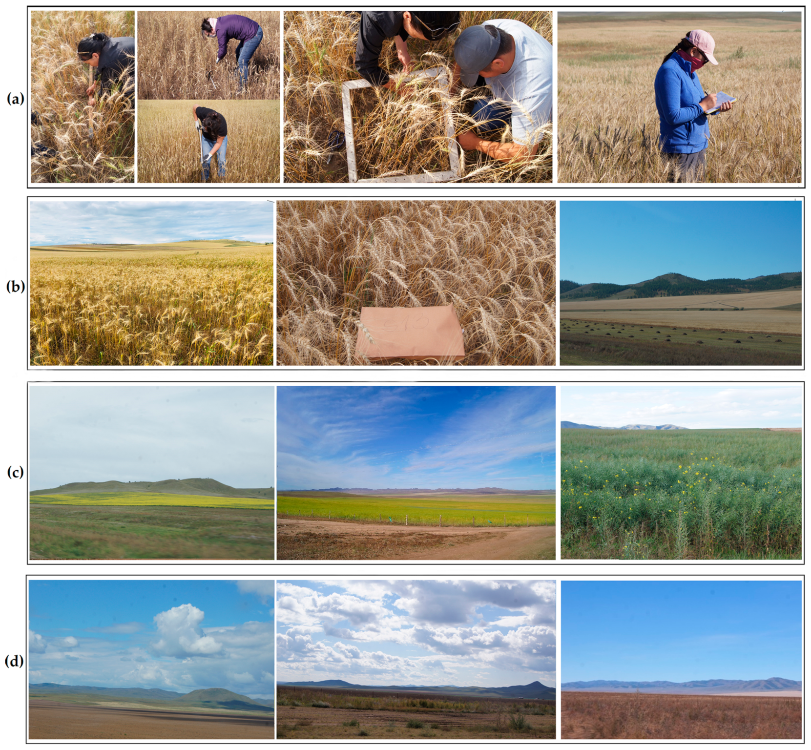
2.2. Collection of Crop Reference Data

Data were collected between the 6 to 26 September 2018, close to the harvest season of the crop (Figure 4). Information collected included geographic location (longitude and latitude), crop-type name, and photos. Samples were collected by the GPS-Video-GIS application (GVG) [53], an all-in-one system of location, photo, and attribute tagging providing quick access to photo information with geolocation and crop-type information. The GVG software is a smartphone application that can be downloaded for free from: https://gvgserver.cropwatch.com.cn/download, accessed on 5 April 2022.

A total of 721 samples were collected, including 508 spring wheat samples, 76 rapeseed samples, and 137 fallow field samples during a 3000 km-long field trip. After completing the field survey, we checked and corrected the position of each sample using high-resolution imagery. Finally, the samples were split into training and validation samples in a ratio of 60:40 for crop classification and accuracy evaluation.

2.3. Satellite Data Processing

In this study, the S1 synthetic aperture radar (SAR) ground range detected (GRD) and S2 top-of-atmosphere (TOA) reflectance images (Level-1C) were used for crop type identification. S1 and S2 were launched by the European Space Agency (ESA). GEE has archived all S1 and S2 data for free use. The S2 optical images cannot provide helpful information in cloudy and rainy weather, while the SAR satellite of S1 can obtain usable images in cloud-covered conditions. Therefore, we used a combination of S1 and S2 images to find the best combination of features to classify crop types and extract crop types in the study area.

2.3.1. Sentinel-2 Data

S2 is a 14-band multispectral acceptable spatial resolution optical image with 4 bands of 10 m (blue, green, red, near-infrared), 6 bands of 20 m (red edge 1, red edge 2, red edge 3, red edge 4, swir1, swir2) and 4 bands of 60 m (aerosol, water vapor, cirrus, cloud cover) spatial resolution. In this study, 20 m reflectances were resampled to 10 m by the nearest-neighbor approach [54]. S2 consists of 2 satellites (2A and 2B) with ten days of revisit time for each satellite and an interception/overlapping period of 5 days for both satellites. S2 TOA Level-1C images were acquired from 11 May to 31 October 2018, followed by cloud-free time-series reconstruction processing. S2 TOA Level-1C data are widely used in crop-type classification and have a minimal impact on crop classification results, such as paddy [27], maize [29], winter wheat [30], and mixed crop types’ identification [31].

(1)

Cloud free

The cloud-masking band of S2 provides information on cloud cover, but studies have shown that it is not as effective when used to remove pixels contaminated by cloud cover [40]. In this study, a modified Luo–Trishchenko–Khlopenkov (LTK) scene identification algorithm [55] designed for Moderate Resolution Imaging Spectroradiometer (MODIS) data was used to clear cloud and shadow of Landsat [55] and S2 [40] data. You et al. [31,40] explained the processing principle of the modified LTK for cloud detection of S2. It uses aerosol, blue, green, and red bands of S2, normalized difference moisture index (NDMI), and normalized difference snow accumulation index (NDSI) to calculate cloud volume and detect cloud layers. This study also employed modified LTK to remove the pixels of S2 contaminated by clouds.

(2)

Time-series reconstruction of metric

Swir1 and Swir2 reflectance bands have a good ability to separate crops [25,31]. Enhanced vegetation index (EVI) [56], green chlorophyll vegetation index (GCVI) [27,57] normalized differential senescent vegetation index (NDSVI) [58], normalized vegetation index (NDVI) [59], red-edge NDVI (RENDVI) [35] and red-edge position (REP) [35] indices were used as features to extract crop types from the study sites. NDVI is an index widely used to identify the distribution of crop types; EVI has a strong ability to overcome the saturation phenomenon during the growing season; RENDVI and REP are red-edge-based indices, both sensitive to crop conditions; and the GCVI index proved to have a strong ability to separate crops. The formulae for NDVI, EVI, GCVI, RENDVI, REP, and NDSVI are summarized below.

EVI = 2.5 × ((Nir − Red)/(Nir + 6 × Red − 7.5 × Blue + 1))

(1)

GCVI = Nir/Green − 1

(2)

NDSVI = (Swir1 − Red)/(Swir1 + Red)

(3)

NDVI = (Nir − Red)/(Nir + Red)

(4)

RENDVI = (Nir − Red2)/(Nir + Red2)

(5)

REP = (705 + 35 × (0.5 × (Red3 + Red) − Red1)/(Red2 − Red1))/1000

(6)

where Nir, Red, Blue, Green, Red1, Red2, Red3, and Swir1 are the reflection bands of S2. The above features are discontinuous due to the cloud cover, increasing crop differentiation difficulty. In this study, the median composite method, linear moving interpolation [38,54] and Savitzky–Golay (SG) filter [39], were utilized to reconstruct the continuous S2 features within a 10-day interval.

In step 1, the time series with a 10-day interval of S2 features are generated by the median composite method, and a total of 18 images for each feature were generated by the median composite method from May to October 2018. The median composite method is easily applied and proved to be superior to the mean composite method by many previous studies [40,60,61].

In step 2, the gap existing in the S2 composite time series is filled by the linear temporal moving interpolation method [31,38,40]. After analyzing the length of the data gaps, we found that the maximum missing data length is 30 days; therefore, the half moving window is set to 3 (equals 30 days, Equation (7)):

$${\mathrm{Index}}_{\mathrm{i}}={\mathrm{Index}}_{\mathrm{k}}+\frac{\left({\mathrm{Index}}_{\mathrm{j}}-{\mathrm{Index}}_{\mathrm{k}}\right)\ast \left({\mathrm{d}}_{\mathrm{i}}-{\mathrm{d}}_{\mathrm{k}}\right)}{({\mathrm{d}}_{\mathrm{j}}-{\mathrm{d}}_{\mathrm{k}})}$$

(7)

where ${\mathrm{Index}}_{\mathrm{i}}$ is the index existing gap, and ${\mathrm{Index}}_{\mathrm{k}}$ and ${\mathrm{Index}}_{\mathrm{j}}$ the good observation before and after ${\mathrm{Index}}_{\mathrm{i}}$. ${\mathrm{d}}_{\mathrm{k}}$, ${\mathrm{d}}_{\mathrm{i}}$, and ${\mathrm{d}}_{\mathrm{j}}$ and day of a year of kth, ith and jth.

Step 3: After filling the gaps in the S2 composite time series, the noise of the S2 time series generated by the linear shift interpolation method is smoothed with an SG filter with a window at 3 × 3. In order to avoid the memory computational error, the smoothed time series is first imported into assets of GEE and then exported to the javascript code.

2.3.2. Sentinel-1 Data

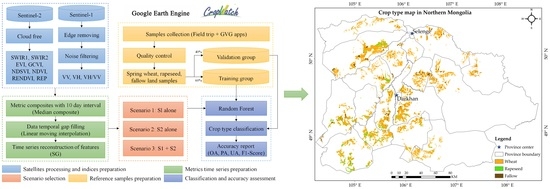
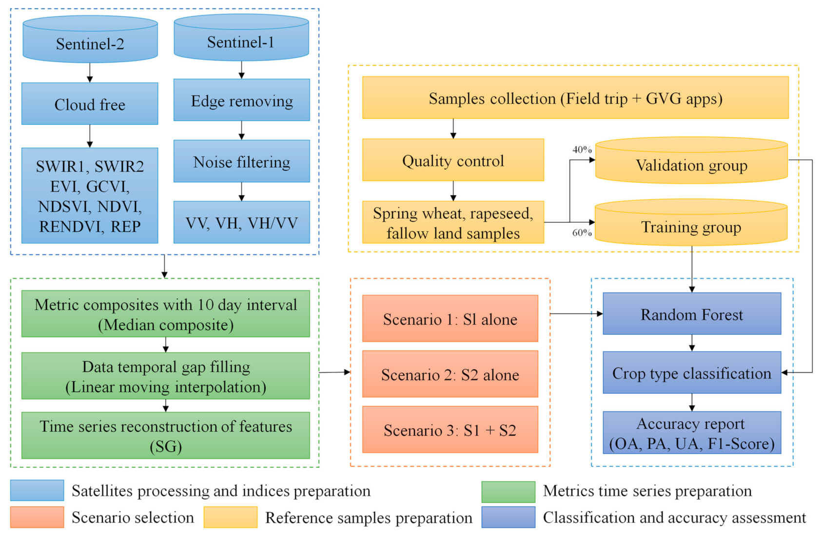
We collected all S1 data from 11 May to 31 October 2018 to determine the crop type for this study. S1 in C band imagery (frequency = 5.4 GHz) globally had a 12 or 6 day revisit cycle depending on 1A and 1B imagery availability. The IW modes of S1 provided dual-polarization with vertical transmit and vertical receive (VV), vertical transmit, and horizontal receive (VH). VV and VH of S1 images with 10 m are widely used in the crop-type classification [34].

S1 in GEE was proceeded by Sentinel-1 Toolbox using the thermal noise removal, radiometric calibration, and terrain correction. The edge of S1 is removed using a ‘connected Components’ method in GEE, which mask groups of neighboring pixels processed with values lower than −25 dB in the VV polarization [34,62]. The noise of VV and VH is filtered by the Refined Lee filter [63]. The backscattering coefficients are converted to decibels (dB) via log scaling (dB = 10 × log10(X)) in GEE. Some studies indicated that the ratio of VH and VV (here defined as VH/VV) is a good index to distinguish crops, but it should be calculated in the natural domain [34]; therefore, this study converts the backscattering coefficients of VH and VV from dB value into the natural value by X = 10 × pow (dB/10), and then calculates VH/VV value. Finally, we used the same approaches introduced in Section 2.3.1 to generate time series of VV, VH, and VH/VV with 10-day intervals. The smoothed VV, VH, and VH/VV time series are also imported into assets of GEE and then exported to the javascript code.

3. Methodology

The crop-type identification framework is illustrated in Figure 5. This framework consists of five modules: satellite processing and indices’ preparation, metrics’ time series preparation, scenario selection, reference samples’ preparation, classification, and accuracy assessment.

3.1. Satellites’ Processing and Indices’ Preparation

The primary role of this module is to process S1 and S2 images and provide them for metrics’ generation. Modified LTK methods eliminate the cloudy pixels in S2 image collection, and then the Swri1 and Swir2 reflectance bands are selected for metrics’ generation. Vegetation indices, including EVI, GCVI, NDSVI, NDVI, RENDVI, and REP, are generated by equations introduced in Section 2.3.1. Because other reflectance bands are used to calculate vegetation indices, they are excluded in crop-type classification to avoid information redundancy. The edge of S1 with IW mode was removed by ‘connected Components’, and then the noise was suppressed by Refined Lee Filter, calculating the VH/VV in the natural domain. Finally, VH, VV bands in the log domain, and VH/VV, were prepared for metrics generation.

3.2. Metrics’ Time-Series Preparation

The function of this module is to provide metrics for crop classification in different cases. Eight S2 features and three S1 features are processed by median synthesis, linear shift interpolation, and SG smoothing methods to generate metrics with an interval of 10 days. The method of time-series reconstruction is described in Section 2.3.1. The method had successfully been applied to crop-type identification in northeast China [31,40]. This module generated 198 features (11 × 18) between 11 May and 31 October 2018.

The M-index [64,65] can determine the ability of a specific characteristic time series to distinguish between two categories. The formula of the M-index can be described as M = |Mean1 − Mean2|/(Std1 + Std2), where Mean1 and Mean2 are the means of the characteristic time series of the first and second class, and Std1 and Std2 are the standard deviations of the characteristic time series of the first and second class. M < 1 indicates difficult separation and M > 1 indicates good separation [64].

3.3. Scenario Selection

Three scenarios were set in the module, namely crop classification with S1 alone, crop classification with S2 alone, and crop classification with S1/S2 together. The performance of the three scenarios will be compared to select the best combination and the earliest and optimal period for crop-type classification in the study areas.

3.4. Reference Samples’ Preparation

The role of this module is to provide training samples for the classifier and to provide validated samples for result accuracy assessment. In this module, the samples of spring wheat, rapeseed, and fallow land are divided into training and validating groups at 60:40. We had 305 samples (spring wheat: 240, rapeseed: 51, fallow land: 14) for training and 208 samples (spring wheat: 168, rapeseed: 32, fallow land: 8) for validation.

3.5. Classification and Accuracy Assessment

3.5.1. Classifier: Random Forest

The random forest (RF) classifier was used to classify the crop types. RF builds multiple trees based on random bootstrapped training data samples [66]. Each tree contains a subset of training data through replacement (a bagging approach), and the nodes are split using the best split variables. Typically, about two-thirds of the samples (in-bag samples) are used for the training tree, while the remaining one-third (out-of-the-bag samples) are used for internal cross-validation techniques to estimate the performance of the RF algorithm [66]. The error estimating process of the RF model is called the out-of-bag (OOB) error. Each decision tree is generated independently without any pruning, and each node is split using a user-defined number of features selected randomly [66]. As many previous studies have proven the excellent performance of RF [42,67], we employ the GEE platform to train and apply an RF classifier to map crop types due to its high performance. We extracted all S1 and S2 features for analysis of crop classification between May and October. To reduce the effect of non-cropping information on the classifier’s crop classification effectiveness, we removed non-cropping satellite imagery with a cropping mask to improve crop classification accuracy [68,69]. The crop cover mask is provided by the IRIMHE in Mongolia [70].

3.5.2. Accuracy Assessment

This study used the RF classifier and the collected field crop-type data for crop-type classification. For each class, 60% of the total points were randomly selected for training, and the remaining 40% of field survey points were used to assess the accuracy. The confusion metrics were used to assess crop-type classification accuracy, including user accuracy (UA), producer accuracy (PA), overall accuracy (OA), Kappa coefficient, and F1-score. These accuracy calculations were presented in the equations below (more details in R. G. Congalton) [71].

$$\mathrm{UA}=\frac{{\mathrm{X}}_{\mathrm{ii}}}{{\mathrm{X}}_{\mathrm{i}+}}$$

(8)

$$\mathrm{PA}=\frac{{\mathrm{X}}_{\mathrm{ii}}}{{\mathrm{X}}_{+\mathrm{i}}}$$

(9)

$$\mathrm{OA}=\frac{{{\displaystyle \sum }}_{\mathrm{i}=1}^{\mathrm{n}}{\mathrm{X}}_{\mathrm{i}+}}{\mathrm{N}}$$

(10)

$$\mathrm{Kappa}=\frac{\mathrm{N}{{\displaystyle \sum }}_{\mathrm{i}=1}^{\mathrm{r}}{\mathrm{X}}_{\mathrm{ii}}-{{\displaystyle \sum }}_{\mathrm{i}=1}^{\mathrm{r}}\left({\mathrm{X}}_{\mathrm{i}+}\times {\mathrm{X}}_{+\mathrm{i}}\right)}{{\mathrm{N}}^2-{{\displaystyle \sum }}_{\mathrm{i}=1}^{\mathrm{r}}\left({\mathrm{X}}_{\mathrm{i}+}\times {\mathrm{X}}_{+\mathrm{i}}\right)}$$

(11)

$$\mathrm{F}1-\mathrm{score}=\frac{2\times \mathrm{UA}\times \mathrm{PA}}{\mathrm{UA}+\mathrm{PA}}$$

(12)

where ${\mathrm{X}}_{\mathrm{ii}}$ is the number of observations in row i and column i, ${\mathrm{X}}_{\mathrm{i}+}$ and ${\mathrm{X}}_{+\mathrm{i}}$ are the marginal totals of row i and column j, and N is the total number of observations.

4. Results

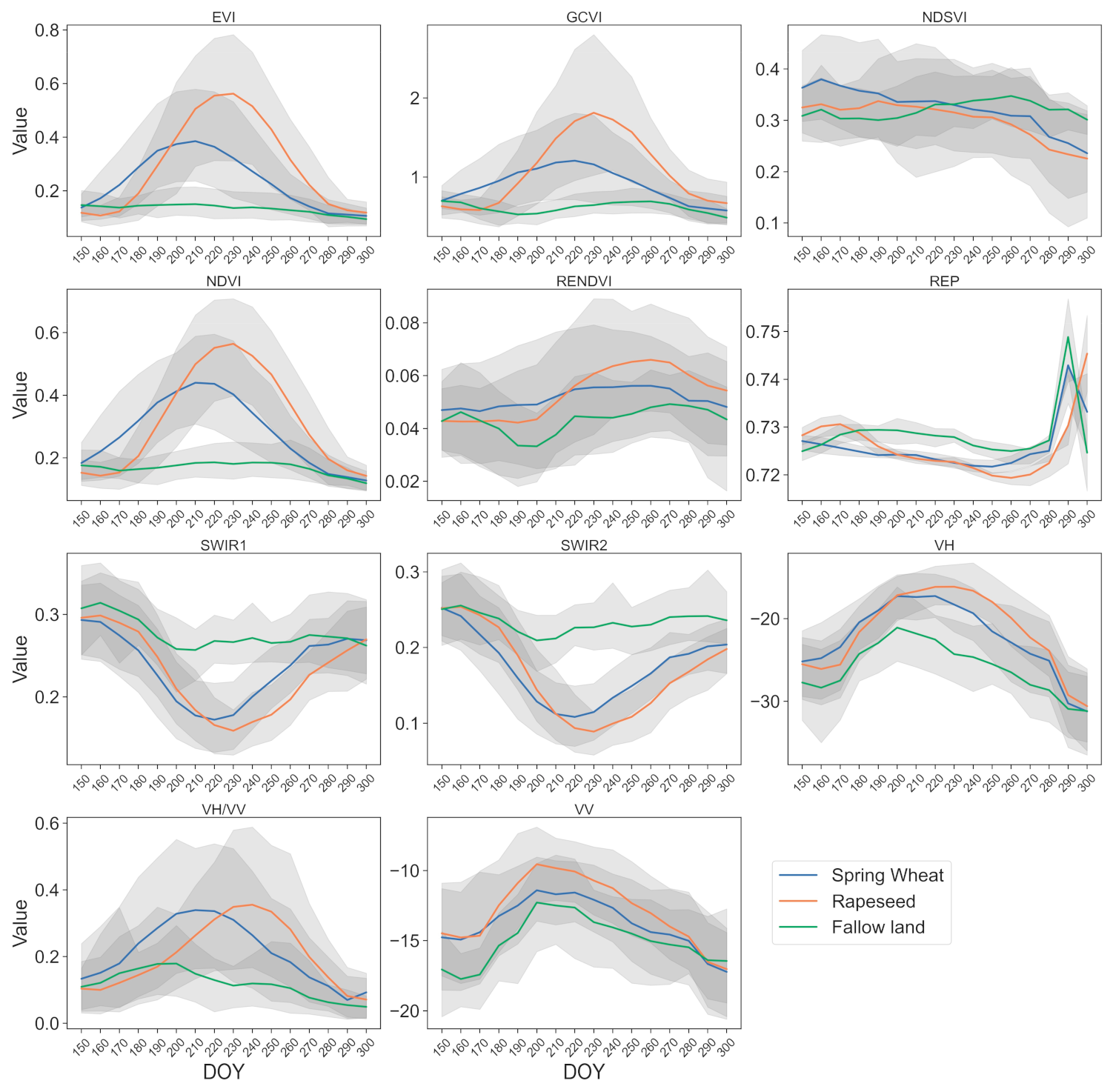
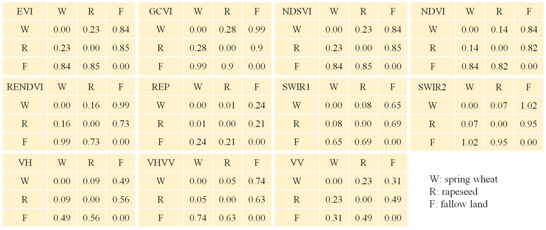
4.1. Temporal of the Satellite Metrics for Crops

Figure 6 shows the 10-day intervals of EVI, GCVI, NDSVI, NDVI, RENDVI, REP, SWIR1, SWIR2, VH, VV, and VH/VV curves for spring wheat, rapeseed, and fallow land. EVI, GCVI, NDVI, and VH/VV curves indicate that spring wheat and rapeseed reached their growth peaks at day 210 of the year (DOY) (late July) and 230 DOY (late August). The difference in NDVI between rapeseed and spring wheat indicates that rapeseed was greener than spring wheat in the study area. The differences in EVI, GCVI, NDVI, and VH/V indicate that they could separate spring wheat and rapeseed, while NDSVI and REP are difficult to separate due to similar curves.

To estimate the separation between spring wheat and rapeseed, we calculated the M values of the 12 indices for spring wheat, rapeseed, and fallow land (Figure 7). The M value between spring wheat and rapeseed was much lower than 1, indicating that separating spring wheat and rapeseed with a single index was challenging. Compared with spring wheat and rapeseed, the M values between fallow and non-fallow lands were relatively high, and the separation between them was better than that between spring wheat and rapeseed.

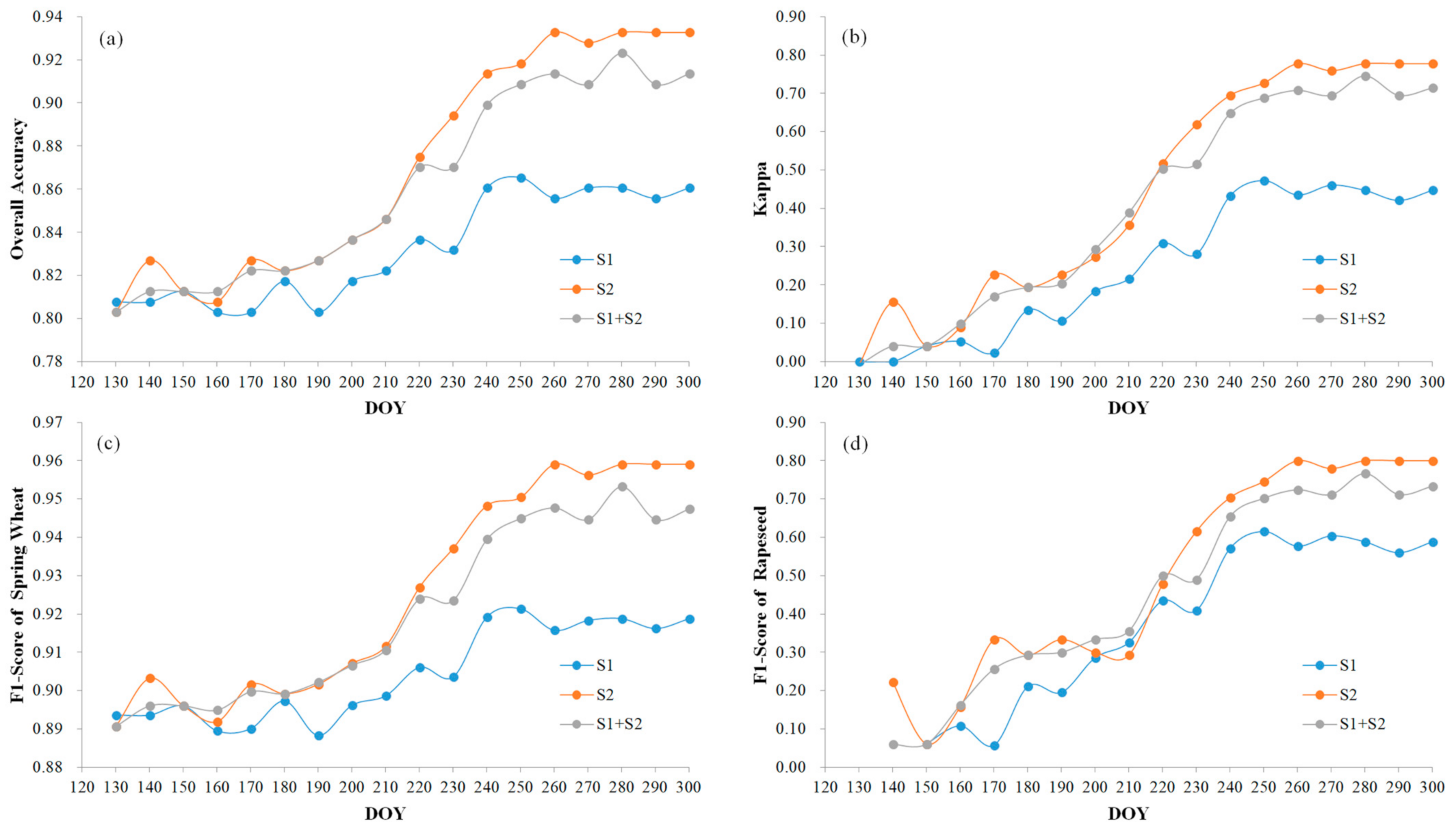
4.2. Accuracy Assessment for Three Scenarios

Figure 8 shows the OA, kappa, and F1-score variation for spring wheat and rapeseed. The OA, kappa, and F1-score increased with the extension of monitoring time length. S2-based crop classification performed best in all three scenarios with the highest OA, kappa, and F1-score. The results of OA, kappa, and F1-score values are shown in Appendix A (

Table A1. Overall accuracy (OA) and Kappa index values for the different classification scenarios.

Date	DOY	Overall Accuracy (OA)			Kappa
		S1	S2	S1 + S2	S1	S2	S1 + S2
11 May 2018	130	0.81	0.80	0.80	0.00	−0.01	−0.01
21 May 2018	140	0.81	0.83	0.81	0.00	0.16	0.04
31 May 2018	150	0.81	0.81	0.81	0.04	0.04	0.04
10 June 2018	160	0.80	0.81	0.81	0.05	0.09	0.10
20 June 2018	170	0.80	0.83	0.82	0.02	0.23	0.17
30 June 2018	180	0.82	0.82	0.82	0.13	0.19	0.19
10 July 2018	190	0.80	0.83	0.83	0.11	0.23	0.20
20 July 2018	200	0.82	0.84	0.84	0.18	0.27	0.29
30 July 2018	210	0.82	0.85	0.85	0.22	0.36	0.39
9 August 2018	220	0.84	0.88	0.87	0.31	0.52	0.50
19 August 2018	230	0.83	0.89	0.87	0.28	0.62	0.52
29 August 2018	240	0.86	0.91	0.90	0.43	0.69	0.65
8 Septermber 2018	250	0.87	0.92	0.91	0.47	0.73	0.69
18 Septermber 2018	260	0.86	0.93	0.91	0.43	0.78	0.71
28 Septermber 2018	270	0.86	0.93	0.91	0.46	0.76	0.69
8 October 2018	280	0.86	0.93	0.92	0.45	0.78	0.75
18 October 2018	290	0.86	0.93	0.91	0.42	0.78	0.69
28 October 2018	300	0.86	0.93	0.91	0.45	0.78	0.71

and

Table A2. F1-score values of spring wheat and rapeseed for the different classification scenarios.

Date	DOY	F1 Score (Spring Wheat)			F1 Score (Rapeseed)
		S1	S2	S1 + S2	S1	S2	S1 + S2
11 May 2018	130	0.89	0.89	0.89
21 May 2018	140	0.89	0.90	0.90		0.22	0.06
31 May 2018	150	0.90	0.90	0.90	0.06	0.06	0.06
10 June 2018	160	0.89	0.89	0.89	0.11	0.16	0.16
20 June 2018	170	0.89	0.90	0.90	0.06	0.33	0.26
30 June 2018	180	0.90	0.90	0.90	0.21	0.29	0.29
10 July 2018	190	0.89	0.90	0.90	0.20	0.33	0.30
20 July 2018	200	0.90	0.91	0.91	0.29	0.30	0.33
30 July 2018	210	0.90	0.91	0.91	0.33	0.29	0.36
9 August 2018	220	0.91	0.93	0.92	0.43	0.48	0.50
19 August 2018	230	0.90	0.94	0.92	0.41	0.62	0.49
29 August 2018	240	0.92	0.95	0.94	0.57	0.70	0.65
8 Septermber 2018	250	0.92	0.95	0.94	0.62	0.75	0.70
18 Septermber 2018	260	0.92	0.96	0.95	0.58	0.80	0.72
28 Septermber 2018	270	0.92	0.96	0.94	0.60	0.78	0.71
8 October 2018	280	0.92	0.96	0.95	0.59	0.80	0.77
18 October 2018	290	0.92	0.96	0.94	0.56	0.80	0.71
28 October 2018	300	0.92	0.96	0.95	0.59	0.80	0.73

). The combination of S1 and S2 was superior to S1 alone for crop classification. A study in Heilongjiang province also found that the accuracy of using S1 only was much lower than the results using S2 and S1 [40]. The change in OA based on S2 indicates that OA increased rapidly from day 190 to day 260, and the largest increase rate (0.029) occurred from 210 DOY to 220 DOY. The same trend was observed in the change in the kappa coefficient. Spring wheat was the dominant crop in the study area. The F1-score of spring wheat was significantly higher than that of rapeseed, and it increased slowly from 0.89 to 0.96; the F1-score remained unchanged after 240 DOY. The F1-score of rapeseed maintained a rapid increase from 140 DOY (F1 = 0.22) to 260 DOY (F1 = 0.80). From 210 DOY (end of July) to 260 DOY (August to mid-September), the F1-score of rapeseed maintained a rapid growth. The curves of Figure 6 indicate that the difference in features increased from 210 DOY to 260 DOY, which can explain the changes in OA, Kappa, and F1-score.

4.3. Classification Results

4.3.1. Accuracy Assessment

OA, kappa, and F1-score indicators show that the best classification results could be achieved between DOY 130 and DOY 260 using S2 data (Figure 9). During this period, OA and kappa were 0.93 and 0.78, respectively; the F1-scores for spring wheat and rapeseed were 0.96 and 0.80, respectively (

Table 1. Accuracy assessment using Sentinel-2 data from 31 May to 18 September 2018.

Name	Spring Wheat	Rapeseed	Fallow Land	PA
Spring wheat	164	4	0	0.98
Rapeseed	8	24	0	0.75
Fallow land	2	0	6	0.75
UA	0.94	0.86	1.00	OA = 0.93, Kappa = 0.78

). PA was 0.98, 0.75, and 0.75 for spring wheat, rapeseed, and fallow. UA was 0.94, 0.86, and 1.00 for spring wheat, rapeseed, and fallow. The largest mixed classification occurred in rapeseed and fallow, one-quarter of which were misclassified as spring wheat.

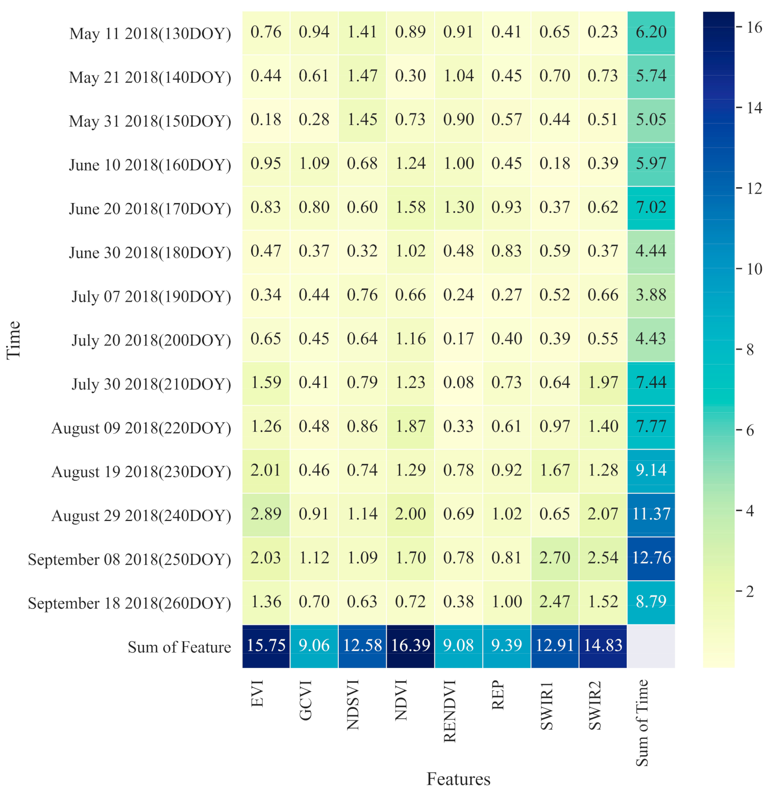
4.3.2. Weight Contribution

Based on the ‘ee.Classifier.explain()’ function of the random forest classifier in GEE, the “ee.Classifier.explain()” function of the random forest classifier in GEE will return a dictionary that includes component of classes, importance, numberOfTrees, outOfBagErrorEstimate, and tree. Importance includes the weight for each metric estimated by the increase in ‘outOfBagError’ when a specific metric dropped. In this study, we normalized the contribution of each metric and obtained the contribution matrix diagrams of the 96 metrics to the crop-type classification for the period between 11 May and 18 September 2018 (Figure 9). In descending order of contribution, the cumulative contribution of NDVI, EVI, SWIR2, SWIR1, NDSVI, REP, RENDVI, and GCVI was 16.39%, 15.75%, 14.83%, 12.91%, 12.58%, 9.39%, 9.08%, and 9.06%, respectively. NDVI, EVI, and SWIR2 play more important roles than other features to classify crop types in the study area. The cumulative contribution of the eight indicators for 130, 140, 150, 160, 170, 180, 190, 200, 210, 220, 230, 240, 250 and 260 DOY was 6.02%, 5.74%, 5.05%, 5.97%, 7.02%, 4.44%, 3.88%, 4.43%, 7.44%, 7.77%, 9.14%, 11.37%, 12.76% and 8.79%. Weight contribution from 210 DOY (30 July) to 260 DOY (18 September) was 57.26%.

4.3.3. Classification Results

We produced and assessed the crop-type map using only the optical images (S2), only SAR (S1), and the combination of SAR (S1) and optical (S2) images in northern Mongolia. The highest accuracy with the crop-type map using S2 satellite data for Selenge and Darkhan Provinces in Mongolia is shown in Figure 10. According to our designed method, the details of crop-type distribution were better extracted (Figure 11). Spring wheat is the main crop in this region. The classification results are divided into three classes, i.e., wheat, rapeseed, and fallow, and the highest OA of the three classes was 93%, respectively. From the analysis, 86.6% of the total cropland area was spring wheat, rapeseed accounted for only 5.7% of the cropland area, and fallow land accounted for 7.7% of the cropland in 2018.

5. Discussion

This study demonstrated 10 m crop-type classification using S1 and S2 data using the RF algorithm in the GEE cloud computing platform in northern Mongolia in 2018. The produced high-resolution crop-type map is essential for sustainable agricultural development, regional food security, crop planting areas, and spatial distribution of crops. In Mongolia, a previous study mapped only croplands at the country level, with a 30 m spatial resolution [70]. However, the classification of the specific crop types is still challenging. This paper proposed and presented an RF classifier approach based on the optimal data combination of S1 and S2. Finally, we generated the crop types map at 10 m spatial resolution in northern Mongolia using S2 alone, which generated the first 10 m spatial resolution crop types in this area.

5.1. Classification Accuracy Compared with Others

The classification results using S2 satellite data have the highest performance. The PA and UA were 0.94 and 0.98, 0.86 and 0.75, and 1 and 0.75 for spring wheat, rapeseed, and fallow land, respectively. The OA and kappa of crop-type classification reached 0.93 and 0.78, respectively. There are many studies on crop classification. For instance, R. Sonobe et al. [72] used 82 vegetation metrics of S2 to identify crop spatial distribution, and the OA obtained by random forest was from 90.2% to 92.2%. R. Saini and S. K. Ghosh et al. [73] have used the S2 optical images to classify crops. The OAs of the classification achieved by RF and SVM using S2 imagery were 84.22% and 81.85%, respectively. Jiang et al. [74] classified crop mapping in China using S2-derived indicators (NDVI, REP, and NDRI). The final results show that the OA of the classified crop map was within 0.94. Immitzer et al. [75] performed crop-type classification using S2 data. The result showed overall accuracies ranging between 65% for tree species and 76% for crop types in Germany. Furthermore, numerous crop type classification and mapping studies are presented based on the Landsat and S2 optical images [32,74,76]. Song and Wang [77] identified the winter wheat planting area using S1 data in North China Plain. The OA reached 84%, and the Kappa coefficient was 0.77, lower than our result. Compared to classification accuracy reported by previous studies, it is evident that our results are acceptable.

5.2. Impact of SAR Information on Crop-Type Classification

Several studies utilized S1 in crop classification to overcome S2 limitations on cloudy days [42,43,44,45,46,47]. However, the OA of classification using only S1 has a lower accuracy than optical imagery-based classifications. In our study, the classification accuracy was only SAR-based and significantly lower than that which was optical-based. Many previous studies have shown that the combination of optical and SAR data provides better discrimination of crops than optical data alone [32,78,79]. For example, K.Van Tricht et al. [32] used joint optical and SAR imagery to classify crop maps in Belgium. They found that the result based on optical and SAR data together outperformed optical or SAR data alone. However, our study achieved the best crop classification using only S2 features. To further validate our results, this study compared the crop classification accuracy of S2 with different combinations of SAR information (VV, VH, and VH/VV) using the best classification period from 11 May to 18 September 2018 (

Table 2. Crop-type accuracy of different S1 combinations with S2 indices.

Indices	OA	Kappa	F1-Score
			Spring Wheat	Rapeseed
S2 + VV	0.91	0.69	0.94	0.71
S2 + VH	0.92	0.72	0.95	0.74
S2 + VH/VV	0.92	0.74	0.95	0.76
S2 + VH + VV	0.91	0.69	0.94	0.70
S2 + VH + VH/VV	0.92	0.73	0.94	0.70
S2 + VV + VH/VV	0.91	0.71	0.95	0.72
S2 + VV + VH + VH/VV	0.91	0.69	0.94	0.71
S2	0.93	0.78	0.96	0.80

). Among the above combinations, the best crop classification results came from the S2 and VH/VV combinations with OA of 0.92, Kappa of 0.74, and F1-score of 0.95 for spring wheat F1-score of 0.76 for rapeseed. The worst crop results came from the S2, VV, VH, and VH/V combinations with OA of 0.91, Kappa of 0.69, and F1-score of 0.94 for spring wheat F1-score of 0.70 for rapeseed. This result shows that the combined use of optical and SAR data does not always yield the best classification results. Our findings are supported by the study of You et al. [40], who found a minimal contribution of S1 to the separation of maize and soybean in Heilongjiang Province, China.

In short, S2-based is the best data combination among three data integration scenarios for crop-type classification in northern Mongolia. Our results with those of other studies indicate that crop-type accuracy varies with study area, and the best data combinations should be compared to each other to achieve the best crop-type classification accuracy.

5.3. Compare to Percentiles Composite of Time-Series Reconstruction

We reconstructed continuous time series of S2 by median synthesis, linear moving interpolation, and SG filters. These time series describe changes in the growth process of spring wheat and rapeseed and capture changes in phenology. Percentile composite is widely used in metric synthesis [27,29] as it is less sensitive to the length and continuity of satellite data [80]. In this study, we used percentile synthesis (percentiles equal 5, 25, 50, 75, 95) to generate metrics for S2 from 130 DOY (11 May) to 260 DOY (18 September) 2018. The OA and kappa were 0.90 and 0.64 based on the percentile approach, respectively, and OA was significantly lower than the 10-day-intervals time-series reconstruction results. This suggested that the 10-day-interval time-series reconstruction performs well in classifying crop types in Mongolia. This can be attributed to the dry climate of Mongolia, which means that the amount of available data is high, and there are fewer missing data values, allowing for better reconstruction of continuous time series.

5.4. Shortcomings

Although good results were achieved in crop-type classification, the F1-score for rapeseed was only 0.80, and about one-quarter of the rapeseed samples were misclassified as spring wheat, meaning that the accuracy of rapeseed classification needs to be improved in the future. Misclassification of wheat and rapeseed is a challenge that needs to be addressed. In the future, a better indicator should be devised to improve the separability of spring wheat and rapeseed. The time-series reconstruction method used in this study achieved good performance in crop-type classification due to the dry climate in the study area. However, its performance in humid regions should be tested robustly.

6. Conclusions

The current study fills a gap in high-spatial-resolution crop types in northern Mongolia and could provide strong support for yield estimation of spring wheat. This study used cloud computing technology to compare crop-type classification using three scenarios (S1 alone, S2 alone, S1 + S2) in northern Mongolia in 2018. The study results show that the S2-based classification results outperformed S1 + S2- and S1-based ones. The classification results improved with increasing monitoring time length, with 130 DOY (11 May) to 260 DOY (18 September) being the best period for crop-type classification, implying that good results can be achieved as early as one month before harvest. Thus, from our results, we recommend using S2 data between 130 DOY and 260 DOY for crop-type classification mapping in northern Mongolia. The crop classification effect improved rapidly from 210 DOY (end of July) to 260 DOY (August to mid-September). Our results also indicate that differences between optical and SAR satellite combinations need to be compared to select the best satellite combination in the crop classification process. Furthermore, our result also indicate that the 10-day-interval data integration outperformed the percentile composites. In short, the framework demonstration in this study can prioritize mitigation plans to support national food security in Mongolia.

References

1. NSO. National Statistic Ofiice of Mongolia. Available online: https://www.1212.mn/stat.aspx?LIST_ID=976_L10_2,%20(15022022) (accessed on 5 April 2022).
2. FAO. Special Report FAO/WFP Crop and Livestock Assessment Mission to Mongilia. Available online: https://reliefweb.int/report/mongolia/special-report-faowfp-crop-and-livestock-assessment-mission-mongolia (accessed on 5 April 2022).
3. Lussem, U.; Hütt, C.; Waldhoff, G. Combined analysis of Sentinel-1 and Rapideye data for improved crop type classification: An early season approach for rapeseed and cereals. ISPRS-Int. Arch. Photogramm. Remote Sens. Spat. Inf. Sci. 2016, XLI-B8, 959–963. [Google Scholar] [CrossRef] [Green Version]
4. Gil, J.D.B.; Reidsma, P.; Giller, K.; Todman, L.; Whitmore, A.; van Ittersum, M. Sustainable development goal 2: Improved targets and indicators for agriculture and food security. Ambio 2019, 48, 685–698. [Google Scholar] [CrossRef] [Green Version]
5. Nilsson, M.; Chisholm, E.; Griggs, D.; Howden-Chapman, P.; McCollum, D.; Messerli, P.; Neumann, B.; Stevance, A.S.; Visbeck, M.; Stafford-Smith, M. Mapping interactions between the sustainable development goals: Lessons learned and ways forward. Sustain. Sci. 2018, 13, 1489–1503. [Google Scholar] [CrossRef] [Green Version]
6. Liang, X.; Li, P.; Wang, J.; Shun Chan, F.K.; Togtokh, C.; Ochir, A.; Davaasuren, D. Research progress of desertification and its prevention in mongolia. Sustainability 2021, 13, 6861. [Google Scholar] [CrossRef]
7. Meng, X.; Gao, X.; Li, S.; Lei, J. Monitoring desertification in Mongolia based on Landsat images and Google Earth Engine from 1990 to 2020. Ecol. Indic. 2021, 129, 107908. [Google Scholar] [CrossRef]
8. Tuvdendorj, B.; Wu, B.; Zeng, H.; Batdelger, G.; Nanzad, L. Determination of appropriate remote sensing indices for spring wheat yield estimation in mongolia. Remote Sens. 2019, 11, 2568. [Google Scholar] [CrossRef] [Green Version]
9. Otgonbayar, M.; Atzberger, C.; Chambers, J.; Amarsaikhan, D.; Böck, S.; Tsogtbayar, J. Land suitability evaluation for agricultural cropland in mongolia using the spatial MCDM method and AHP based GIS. J. Geosci. Environ. Prot. 2017, 5, 238–263. [Google Scholar] [CrossRef] [Green Version]
10. Myagmartseren, P.; Myagmarjav, I. Cropland suitability assessment and confusion matrix evaluation with GIS. Mong. J. Agric. Sci. 2018, 21, 78–83. [Google Scholar] [CrossRef]
11. Natsagdorj, E.; Renchin, T.; de Maeyer, P.; Dari, C.; Tseveen, B. Long-term soil moisture content estimation using satellite and climate data in agricultural area of Mongolia. Geocarto Int. 2019, 34, 722–734. [Google Scholar] [CrossRef]
12. Nandintsetseg, B.; Shinoda, M. Seasonal change of soil moisture in Mongolia: Its climatology. Int. J. Climatol. 2010, 1152, 1143–1152. [Google Scholar] [CrossRef]
13. Nanzad, L.; Zhang, J.; Tuvdendorj, B.; Nabil, M.; Zhang, S.; Bai, Y. NDVI anomaly for drought monitoring and its correlation with climate factors over Mongolia from 2000 to 2016. J. Arid Environ. 2019, 164, 69–77. [Google Scholar] [CrossRef]
14. Kang, Y.; Guo, E.L.; Wang, Y.F.; Bao, Y.L.; Bao, Y.H.; Na, R.M. Application of temperature vegetation dryness index for drought monitoring in Mongolian Plateau. Appl. Ecol. 2021, 32, 2534–2544. [Google Scholar] [CrossRef]
15. Norovsuren, B.; Tseveen, B.; Batomunkuev, V.; Renchin, T.; Natsagdorj, E.; Yangiv, A.; Mart, Z. Land cover classification using maximum likelihood method (2000 and 2019) at Khandgait valley in Mongolia. IOP Conf. Ser. Earth Environ. Sci. 2019, 381, 012054. [Google Scholar] [CrossRef]
16. Wang, J.; Wei, H.; Cheng, K.; Ochir, A.; Shao, Y.; Yao, J.; Wu, Y.; Han, X.; Davaasuren, D.; Chonokhuu, S.; et al. Updatable dataset revealing decade changes in land cover types in Mongolia. Geosci. Data J. 2022, 1–14. [Google Scholar] [CrossRef]
17. Wardlow, B.; Egbert, S.; Kastens, J. Analysis of time-series MODIS 250 m vegetation index data for crop classification in the U.S. Central Great Plains. Remote Sens. Environ. 2007, 108, 290–310. [Google Scholar] [CrossRef] [Green Version]
18. Blickensdörfer, L.; Schwieder, M.; Pflugmacher, D.; Nendel, C.; Erasmi, S.; Hostert, P. Mapping of crop types and crop sequences with combined time series of Sentinel-1, Sentinel-2 and Landsat 8 data for Germany. Remote Sens. Environ. 2022, 269, 112831. [Google Scholar] [CrossRef]
19. Ghassemi, B.; Dujakovic, A.; Żółtak, M.; Immitzer, M.; Atzberger, C.; Vuolo, F. Designing a european-wide crop type mapping approach based on machine learning algorithms using LUCAS field survey and sentinel-2 data. Remote Sens. 2022, 14, 541. [Google Scholar] [CrossRef]
20. Hunt, M.L.; Blackburn, G.A.; Carrasco, L.; Redhead, J.W.; Rowland, C.S. High resolution wheat yield mapping using Sentinel-2. Remote Sens. Environ. 2019, 233, 111410. [Google Scholar] [CrossRef]
21. Kussul, N.; Lemoine, G.; Gallego, F.J.; Skakun, S.V.; Lavreniuk, M.; Shelestov, A.Y. Parcel-based crop classification in ukraine using landsat-8 data and sentinel-1A data. IEEE J. Sel. Top. Appl. Earth Obs. Remote Sens. 2016, 9, 2500–2508. [Google Scholar] [CrossRef]
22. Gorelick, N.; Hancher, M.; Dixon, M.; Ilyushchenko, S.; Thau, D.; Moore, R. Google earth engine: Planetary-scale geospatial analysis for everyone. Remote Sens. Environ. 2017, 202, 18–27. [Google Scholar] [CrossRef]
23. Yang, J.; Huang, X. The 30 m annual land cover dataset and its dynamics in China from 1990 to 2019. Earth Syst. Sci. Data 2021, 13, 3907–3925. [Google Scholar] [CrossRef]
24. Kumari, N.; Srivastava, A.; Dumka, U.C. A long-term spatiotemporal analysis of vegetation greenness over the himalayan region using google earth engine. Climate 2021, 9, 109. [Google Scholar] [CrossRef]
25. Elnashar, A.; Zeng, H.; Wu, B.; Fenta, A.A.; Nabil, M.; Duerler, R. Soil erosion assessment in the Blue Nile Basin driven by a novel RUSLE-GEE framework. Sci. Total Environ. 2021, 793, 48466. [Google Scholar] [CrossRef] [PubMed]
26. Elnashar, A.; Zeng, H.; Wu, B.; Gebremicael, T.G.; Marie, K. Assessment of environmentally sensitive areas to desertification in the Blue Nile Basin driven by the MEDALUS-GEE framework. Sci. Total Environ. 2022, 185, 152925. [Google Scholar] [CrossRef]
27. Zhang, X.; Wu, B.; Ponce-Campos, G.; Zhang, M.; Chang, S.; Tian, F. Mapping up-to-date paddy rice extent at 10 M resolution in China through the integration of optical and synthetic aperture radar images. Remote Sens. 2018, 10, 1200. [Google Scholar] [CrossRef] [Green Version]
28. Xiao, W.; Xu, S.; He, T. Mapping paddy rice with sentinel-1/2 and phenology-, object-based algorithm—A implementation in hangjiahu plain in China using GEE platform. Remote Sens. 2021, 13, 990. [Google Scholar] [CrossRef]
29. Tian, F.; Wu, B.; Zeng, H.; Zhang, X.; Xu, J. Efficient identification of corn cultivation area with multitemporal synthetic aperture radar and optical images in the google earth engine cloud platform. Remote Sens. 2019, 11, 629. [Google Scholar] [CrossRef] [Green Version]
30. Yang, G.; Yu, W.; Yao, X.; Zheng, H.; Cao, Q.; Zhu, Y.; Cao, W.; Cheng, T. AGTOC: A novel approach to winter wheat mapping by automatic generation of training samples and one-class classification on google earth engine. Int. J. Appl. Earth Obs. Geoinf. 2021, 102, 102446. [Google Scholar] [CrossRef]
31. You, N.; Dong, J.; Huang, J.; Du, G.; Zhang, G.; He, Y.; Yang, T.; Di, Y.; Xiao, X. The 10-m crop type maps in Northeast China during 2017–2019. Sci. Data 2021, 8, 41. [Google Scholar] [CrossRef]
32. van Tricht, K.; Gobin, A.; Gilliams, S.; Piccard, I. Synergistic use of radar sentinel-1 and optical sentinel-2 imagery for crop mapping: A case study for belgium. Remote Sens. 2018, 10, 1642. [Google Scholar] [CrossRef] [Green Version]
33. Dong, J.; Xiao, X.; Menarguez, M.A.; Zhang, G.; Qin, Y.; Thau, D.; Biradar, C.; Moore, B. III. Mapping paddy rice planting area in northeastern Asia with landsat 8 images, phenology-based algorithm and google earth engine. Remote Sens. Environ. 2016, 185, 142–154. [Google Scholar] [CrossRef] [PubMed] [Green Version]
34. d’Andrimont, R.; Verhegghen, A.; Lemoine, G.; Kempeneers, P.; Meroni, M.; van der Velde, M. From parcel to continental scale—A first European crop type map based on sentinel-1 and LUCAS copernicus in-situ observations. Remote Sens. Environ. 2019, 266, 112708. [Google Scholar] [CrossRef]
35. Defourny, P.; Bontemps, S.; Bellemans, N.; Cara, C.; Dedieu, G.; Guzzonato, E.; Hagolle, O.; Inglada, J.; Nicola, L.; Rabaute, T.; et al. Near real-time agriculture monitoring at national scale at parcel resolution: Performance assessment of the Sen2-Agri automated system in various cropping systems around the world. Remote Sens. Environ. 2019, 221, 551–568. [Google Scholar] [CrossRef]
36. Wang, C.; Wang, S.; Cui, H.; Šebela, M.B.; Zhang, C.; Gu, X.; Fang, X.; Hu, Z.; Tang, Q.; Wang, Y. Framework to create cloud-free remote sensing data using passenger aircraft as the platform. IEEE J. Sel. Top. Appl. Earth Obs. Remote Sens. 2021, 14, 6923–6936. [Google Scholar] [CrossRef]
37. Tahsin, S.; Medeiros, S.; Hooshyar, M.; Singh, A. Optical cloud pixel recovery via machine learning. Remote Sens. 2017, 9, 527. [Google Scholar] [CrossRef] [Green Version]
38. Griffiths, P.; Nendel, C.; Hostert, P. Intra-annual reflectance composites from sentinel-2 and landsat for national-scale crop and land cover mapping. Remote Sens. Environ. 2019, 220, 135–151. [Google Scholar] [CrossRef]
39. Chen, J.; Jönsson, P.; Tamura, M.; Gu, Z.; Matsushita, B.; Eklundh, L. A simple method for reconstructing a high-quality NDVI time-series data set based on the savitzky–golay filter. Remote Sens. Environ. 2004, 91, 332–344. [Google Scholar] [CrossRef]
40. You, N.; Dong, J. Examining earliest identifiable timing of crops using all available sentinel 1/2 imagery and google earth engine. ISPRS J. Photogramm. Remote Sens. 2020, 161, 109–123. [Google Scholar] [CrossRef]
41. Zhao, H.; Chen, Z.; Jiang, H.; Jing, W.; Sun, L.; Feng, M. Evaluation of Three deep learning models for early crop classification using sentinel-1a imagery time series—A case study in Zhanjiang, China. Remote Sens. 2019, 11, 2673. [Google Scholar] [CrossRef] [Green Version]
42. Singha, M.; Dong, J.; Zhang, G.; Xiao, X. High resolution paddy rice maps in cloud-prone Bangladesh and Northeast India using Sentinel-1 data. Sci. Data 2019, 6, 26. [Google Scholar] [CrossRef]
43. Arias, M.; Campo-Bescos, M.A.; Alvarez-Mozos, J. Crop type mapping based on sentinel-1 backscatter time series. In Proceedings of the IGARSS 2018—2018 IEEE International Geoscience and Remote Sensing Symposium, Valencia, Spain, 22–27 July 2018; pp. 6623–6626. [Google Scholar] [CrossRef]
44. Arias, M.; Campo-Bescós, M.Á.; Álvarez-Mozos, J. Crop classification based on temporal signatures of sentinel-1 observations over Navarre province, Spain. Remote Sens. 2020, 12, 278. [Google Scholar] [CrossRef] [Green Version]
45. Nguyen, D.B.; Gruber, A.; Wagner, W. Mapping rice extent and cropping scheme in the mekong delta using sentinel-1A data. Remote Sens. Lett. 2016, 7, 1209–1218. [Google Scholar] [CrossRef]
46. Shelestov, A.; Lavreniuk, M.; Vasiliev, V.; Shumilo, L.; Kolotii, A.; Yailymov, B.; Kussul, N.; Yailymova, H. Cloud approach to automated crop classification using sentinel-1 imagery. IEEE Trans. Big Data 2019, 6, 572–582. [Google Scholar] [CrossRef]
47. Nasrallah, A.; Baghdadi, N.; El Hajj, M.; Darwish, T.; Belhouchette, H.; Faour, G.; Darwich, S.; Mhawej, M. Sentinel-1 data for winter wheat phenology monitoring and mapping. Remote Sens. 2019, 11, 2228. [Google Scholar] [CrossRef] [Green Version]
48. Singh, J.; Devi, U.; Hazra, J.; Kalyanaraman, S. Crop-identification using sentinel-1 and sentinel-2 data for Indian region. In Proceedings of the IGARSS 2018—2018 IEEE International Geoscience and Remote Sensing Symposium, Valencia, Spain, 22–27 July 2018; pp. 5312–5314. [Google Scholar] [CrossRef]
49. Behzad, A.; Aamir, M. Estimation of wheat area using sentinel-1 and sentinel-2 datasets (a comparative analysis). Int. J. Agric. Sustain. Dev. 2019, 1, 81–93. [Google Scholar] [CrossRef]
50. Hu, Y.; Zeng, H.; Tian, F.; Zhang, M.; Wu, B.; Gilliams, S.; Li, S.; Li, Y.; Lu, Y.; Yang, H. An interannual transfer learning approach for crop classification in the Hetao Irrigation district, China. Remote Sens. 2022, 14, 1208. [Google Scholar] [CrossRef]
51. van Niel, T.G.; McVicar, T.R. Determining temporal windows for crop discrimination with remote sensing: A case study in south-eastern Australia. Comput. Electron. Agric. 2004, 45, 91–108. [Google Scholar] [CrossRef]
52. Azar, R.; Villa, P.; Stroppiana, D.; Crema, A.; Boschetti, M.; Brivio, P.A. Assessing in-season crop classification performance using satellite data: A test case in Northern Italy. Eur. J. Remote Sens. 2016, 49, 361–380. [Google Scholar] [CrossRef] [Green Version]
53. AIRCAS. Gvg for Android. Available online: https://apkpure.com/gvg/com.sysapk.gvg (accessed on 5 April 2022).
54. Tran, K.H.; Zhang, H.K.; McMaine, J.T.; Zhang, X.; Luo, D. 10 m crop type mapping using Sentinel-2 reflectance and 30 m cropland data layer product. Int. J. Appl. Earth Obs. Geoinf. 2022, 107, 102692. [Google Scholar] [CrossRef]
55. Oreopoulos, L.; Wilson, M.J.; Várnai, T. Implementation on landsat data of a simple cloud-mask algorithm developed for MODIS land bands. IEEE Geosci. Remote Sens. Lett. 2011, 8, 597–601. [Google Scholar] [CrossRef] [Green Version]
56. Huete, A.; Didan, K.; Miura, T.; Rodriguez, E.P.; Gao, X.; Ferreira, L.G. Overview of the radiometric and biophysical performance of the MODIS vegetation indices. Remote Sens. Environ. 2002, 83, 195–213. [Google Scholar] [CrossRef]
57. Gitelson, A.A. Remote estimation of canopy chlorophyll content in crops. Geophys. Res. Lett. 2005, 32, L08403. [Google Scholar] [CrossRef] [Green Version]
58. Zhong, L.; Gong, P.; Biging, G.S. Efficient corn and soybean mapping with temporal extendability: A multi-year experiment using landsat imagery. Remote Sens. Environ. 2014, 140, 1–13. [Google Scholar] [CrossRef]
59. Tucker, C.J. Red and photographic infrared linear combinations for monitoring vegetation. Remote Sens. Environ. 1979, 8, 127–150. [Google Scholar] [CrossRef] [Green Version]
60. Roy, D.P.; Wulder, M.A.; Loveland, T.R.; Woodcock, C.E.; Allen, R.G.; Anderson, M.C.; Helder, D.; Irons, J.R.; Johnson, D.M.; Kennedy, R.; et al. Landsat-8: Science and product vision for terrestrial global change research. Remote Sens. Environ. 2014, 145, 154–172. [Google Scholar] [CrossRef] [Green Version]
61. Teluguntla, P.; Thenkabail, P.S.; Oliphant, A.; Xiong, J.; Gumma, M.K.; Congalton, R.G.; Yadav, K.; Huete, A. A 30-m landsat-derived cropland extent product of Australia and China using random forest machine learning algorithm on Google Earth Engine cloud computing platform. ISPRS J. Photogramm. Remote Sens. 2018, 144, 325–340. [Google Scholar] [CrossRef]
62. d’Andrimont, R.; Lemoine, G.; van der Velde, M. Targeted grassland monitoring at parcel level using sentinels, street-level images and field observations. Remote Sens. 2018, 10, 1300. [Google Scholar] [CrossRef] [Green Version]
63. Lee, J.-S. Refined filtering of image noise using local statistics. Comput. Graph. Image Process. 1981, 15, 380–389. [Google Scholar] [CrossRef]
64. Kaufman, Y.J. Detection of forests using mid-IR reflectance: An application for aerosol studies. IEEE Trans. Geosci. Remote Sens. 1994, 32, 672–683. [Google Scholar] [CrossRef]
65. Xun, L.; Zhang, J.; Cao, D.; Yang, S.; Yao, F. A novel cotton mapping index combining Sentinel-1 SAR and Sentinel-2 multispectral imagery. ISPRS J. Photogramm. Remote Sens. 2021, 181, 148–166. [Google Scholar] [CrossRef]
66. Breiman, L. Random forests. Mach. Learn. 2001, 45, 5–32. [Google Scholar] [CrossRef] [Green Version]
67. Belgiu, M.; Drăguţ, L. Random forest in remote sensing: A review of applications and future directions. ISPRS J. Photogramm. Remote Sens. 2016, 114, 24–31. [Google Scholar] [CrossRef]
68. Khabbazan, S.; Vermunt, P.; Steele-Dunne, S.; Ratering Arntz, L.; Marinetti, C.; van der Valk, D.; Iannini, L.; Molijn, R.; Westerdijk, K.; van der Sande, C. Crop monitoring using sentinel-1 data: A case study from The Netherlands. Remote Sens. 2019, 11, 1887. [Google Scholar] [CrossRef] [Green Version]
69. Chakhar, A. Assessing the accuracy of multiple classification algorithms for crop classification using landsat-8 and sentinel-2 data. Remote Sens. 2020, 12, 1735. [Google Scholar] [CrossRef]
70. Elbegjargal, N.; Khudulmur, N.; Tsogtbaatar, S.; Dash, J.; Mandakh, D. Desertification Atlas of Mongolia; Institute of Geoecology, Mongolian Academy of Sciences: Ulaanbaatar, Mongolia, 2014. [Google Scholar]
71. Congalton, R.G. A review of assessing the accuracy of classifications of remotely sensed data. Remote Sens. Environ. 1991, 37, 35–46. [Google Scholar] [CrossRef]
72. Sonobe, R.; Yamaya, Y.; Tani, H.; Wang, X.; Kobayashi, N.; Mochizuki, K. Crop classification from sentinel-2- derived vegetation indices using ensemble learning. J. Appl. Remote Sens. 2018, 12, 17. [Google Scholar] [CrossRef] [Green Version]
73. Saini, R.; Ghosh, S.K. Crop classification on single date Sentinel-2 imagery using random forest and suppor vector machine. ISPRS-Int. Arch. Photogramm. Remote Sens. Spat. Inf. Sci. 2018, XLII–5, 683–688. [Google Scholar] [CrossRef] [Green Version]
74. Jiang, Y.; Lu, Z.; Li, S.; Lei, Y.; Chu, Q.; Yin, X.; Chen, F. Large-scale and high-resolution crop mapping in China using sentinel-2 satellite imagery. Agriculture 2020, 10, 433. [Google Scholar] [CrossRef]
75. Immitzer, M.; Vuolo, F.; Atzberger, C. First experience with sentinel-2 data for crop and tree species classifications in central Europe. Remote Sens. 2016, 8, 166. [Google Scholar] [CrossRef]
76. Ustuner, M.; Sanli, F.B.; Abdikan, S.; Esetlili, M.T.; Kurucu, Y. Crop typw classification using vegetation indices of Rapideye imagery. ISPRS-Int. Arch. Photogramm. Remote Sens. Spat. Inf. Sci. 2014, XL-7, 195–198. [Google Scholar] [CrossRef] [Green Version]
77. Song, Y.; Wang, J. Mapping Winter Wheat Planting Area and Monitoring Its Phenology Using Sentinel-1 Backscatter Time Series. Remote Sens. 2019, 11, 449. [Google Scholar] [CrossRef] [Green Version]
78. Forkuor, G.; Conrad, C.; Thiel, M.; Ullmann, T.; Zoungrana, E. Integration of optical and synthetic aperture radar imagery for improving crop mapping in Northwestern Benin, West Africa. Remote Sens. 2014, 6, 6472–6499. [Google Scholar] [CrossRef] [Green Version]
79. Inglada, J.; Vincent, A.; Arias, M.; Marais-Sicre, C. Improved early crop type identification by joint use of high temporal resolution sar and optical image time series. Remote Sens. 2016, 8, 362. [Google Scholar] [CrossRef] [Green Version]
80. Zeng, H.; Wu, B.; Wang, S.; Musakwa, W.; Tian, F.; Mashimbye, Z.E.; Poona, N.; Syndey, M. A Synthesizing land-cover classification method based on google earth engine: A case study in Nzhelele and Levhuvu Catchments, South Africa. Chin. Geogr. Sci. 2020, 30, 397–409. [Google Scholar] [CrossRef]
Figure 1. Geographical location of the study area and spatial distribution of collected crop samples (a), Digital Elevation Model (DEM) of Mongolia (b), and Training and validation samples (c).
Remotesensing 14 01830 g001
Figure 2. Annual variation of monthly maximum and minimum temperature, and monthly precipitation for 2018.
Remotesensing 14 01830 g002
Figure 3. Crop calendar of spring wheat and rapeseed in the study area.
Remotesensing 14 01830 g003
Figure 4. Glimpses of field measurements. (a) field measurement; (b) field photographs of wheat; (c) field photographs of rapeseed; (d) field photographs of fallow land.
Remotesensing 14 01830 g004
Figure 5. Flowchart of crop classification.
Remotesensing 14 01830 g005
Figure 6. Temporal profile of remote sensing indicators for spring wheat, rapeseed, and fallow land (Note: the grey represents the standard deviation of indicators for specific DOY).
Remotesensing 14 01830 g006
Figure 7. The M value between spring wheat, rapeseed, and fallow land for 12 features (W, R, and F represent spring wheat, rapeseed, and fallow land, respectively).
Remotesensing 14 01830 g007
Figure 8. The OA, Kappa, and F1-Score variation under three scenarios. (a) OA change; (b) kappa coefficient change; (c) F1-score of spring wheat; (d) F1-score of rapeseed.
Remotesensing 14 01830 g008
Figure 9. Contribution of metrics to crop-type classification.
Remotesensing 14 01830 g009
Figure 10. Crop-type distribution in Selenge and Darkhan provinces of Mongolia.
Remotesensing 14 01830 g010
Figure 11. The detail of crop-type distribution in Selenge and Darkhan provinces of Mongolia.
Remotesensing 14 01830 g011