Author Contributions
Conceptualization, K.B., M.M.; methodology, K.B.; software, K.B.; validation, M.M., M.G. and H.R.; formal analysis, K.B.; investigation, K.B.; resources, M.M., K.B., M.G.; data curation, M.M.; writing—original draft preparation, K.B.; writing—review and editing, M.M.; visualization, K.B.; supervision, H.R., M.G.; funding acquisition, H.R. All authors have read and agreed to the published version of the manuscript.
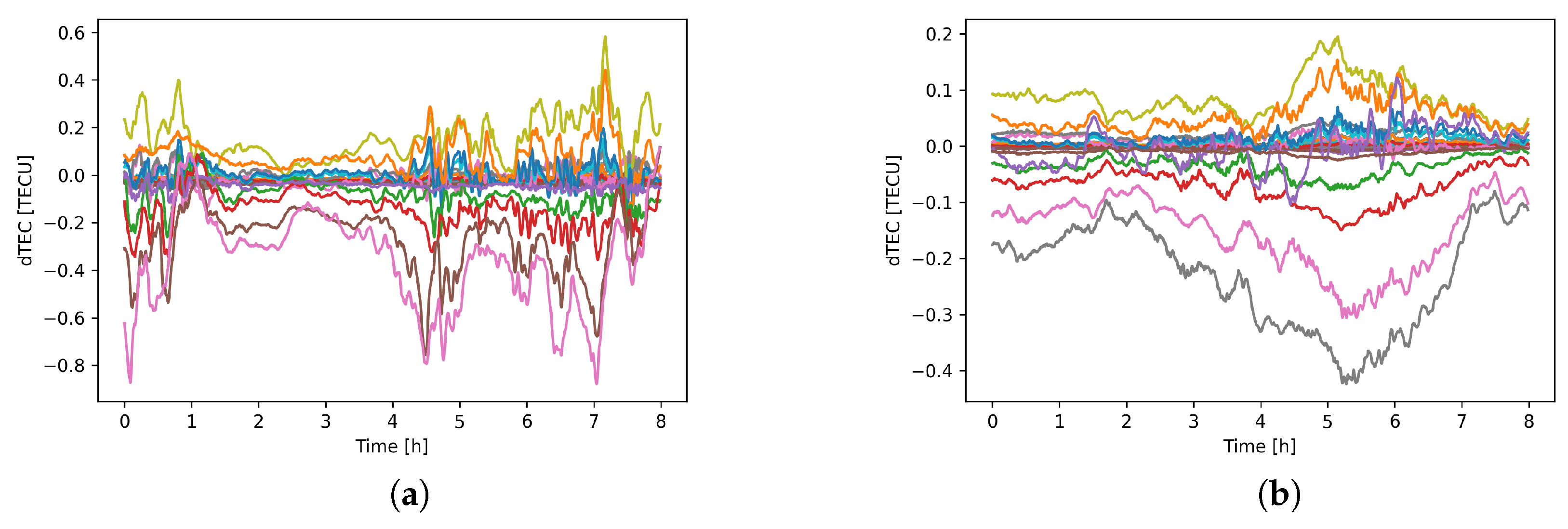
Figure 1.
Differential Total Electron Content (dTEC) variations with time for LOFAR baselines; (a) observation L79324, (b) observation L82655.
Figure 1.
Differential Total Electron Content (dTEC) variations with time for LOFAR baselines; (a) observation L79324, (b) observation L82655.
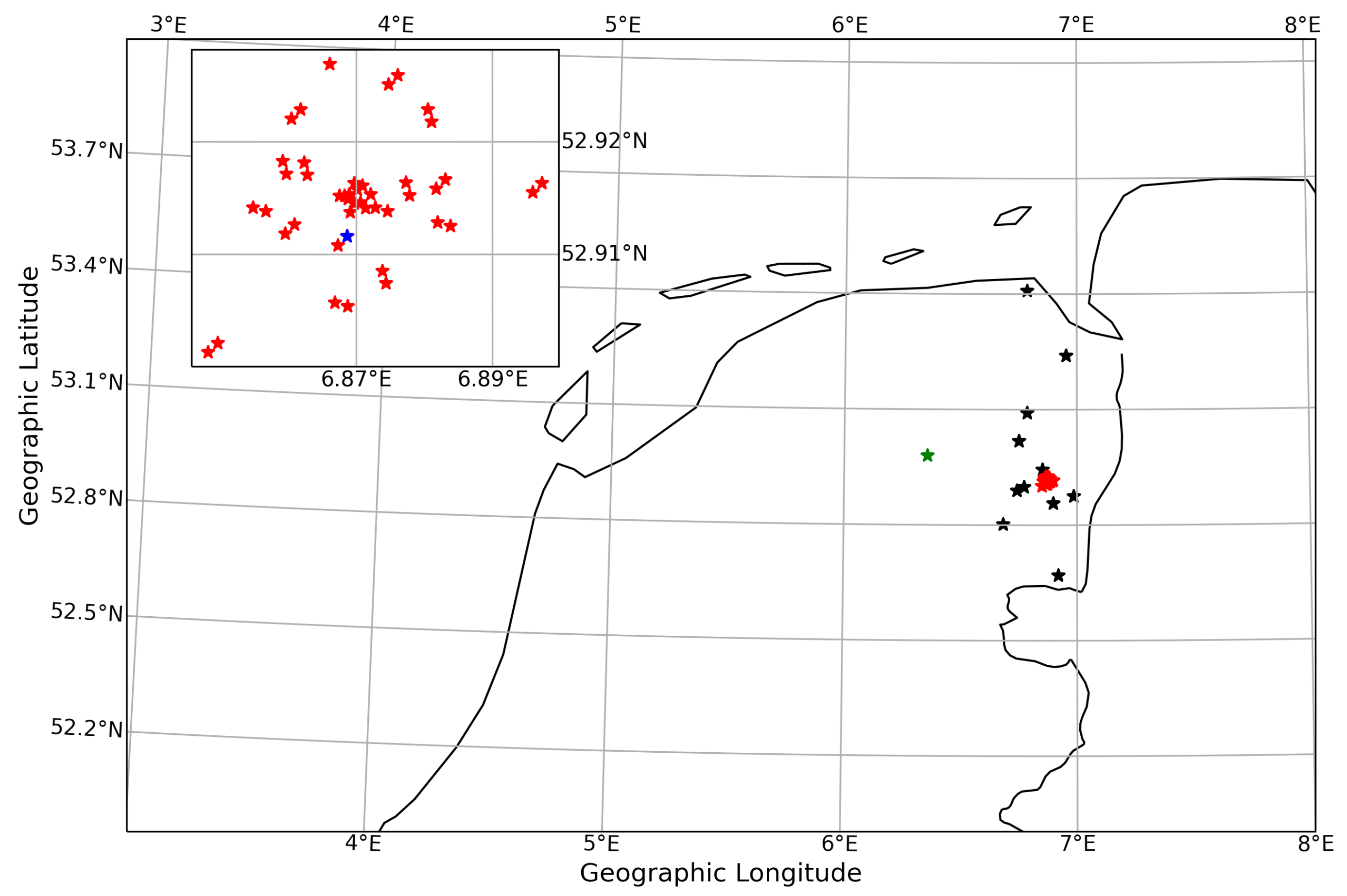
Figure 2.
LOFAR stations’ location; black stars denote remote stations, red stars: core stations, green star: additional station of L82655 observation (see text). Blue star in the inset map shows the reference station.
Figure 2.
LOFAR stations’ location; black stars denote remote stations, red stars: core stations, green star: additional station of L82655 observation (see text). Blue star in the inset map shows the reference station.
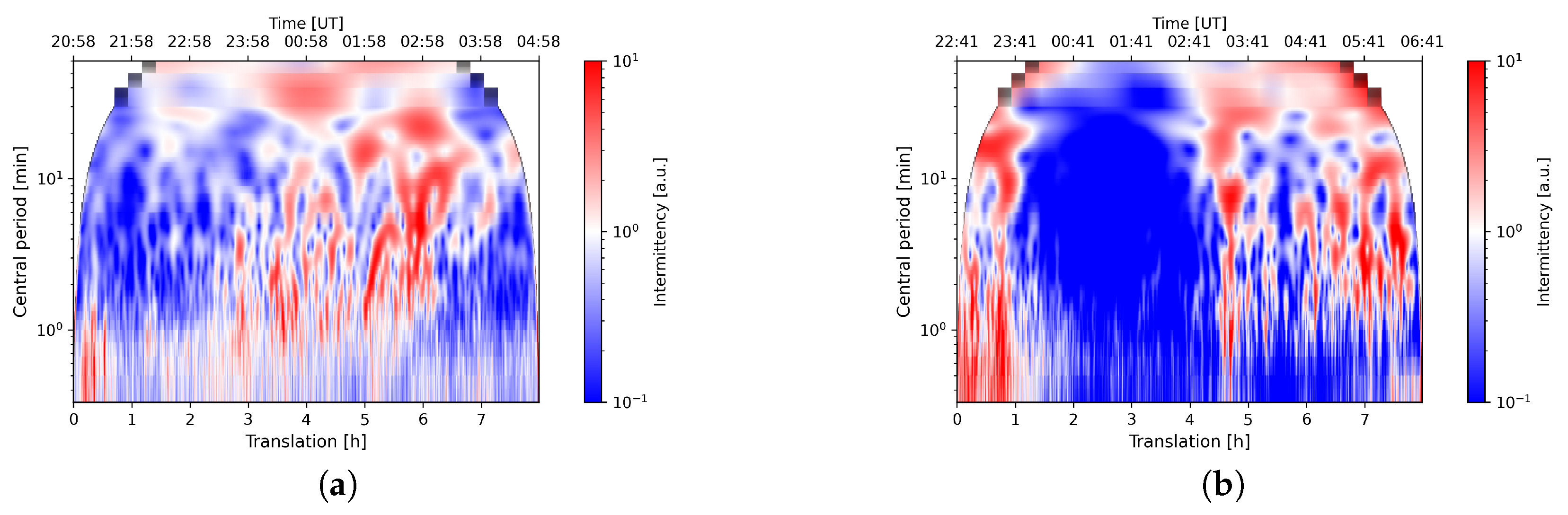
Figure 3.
Intermittency for observations (a) L82655, (b) L79324.
Figure 3.
Intermittency for observations (a) L82655, (b) L79324.
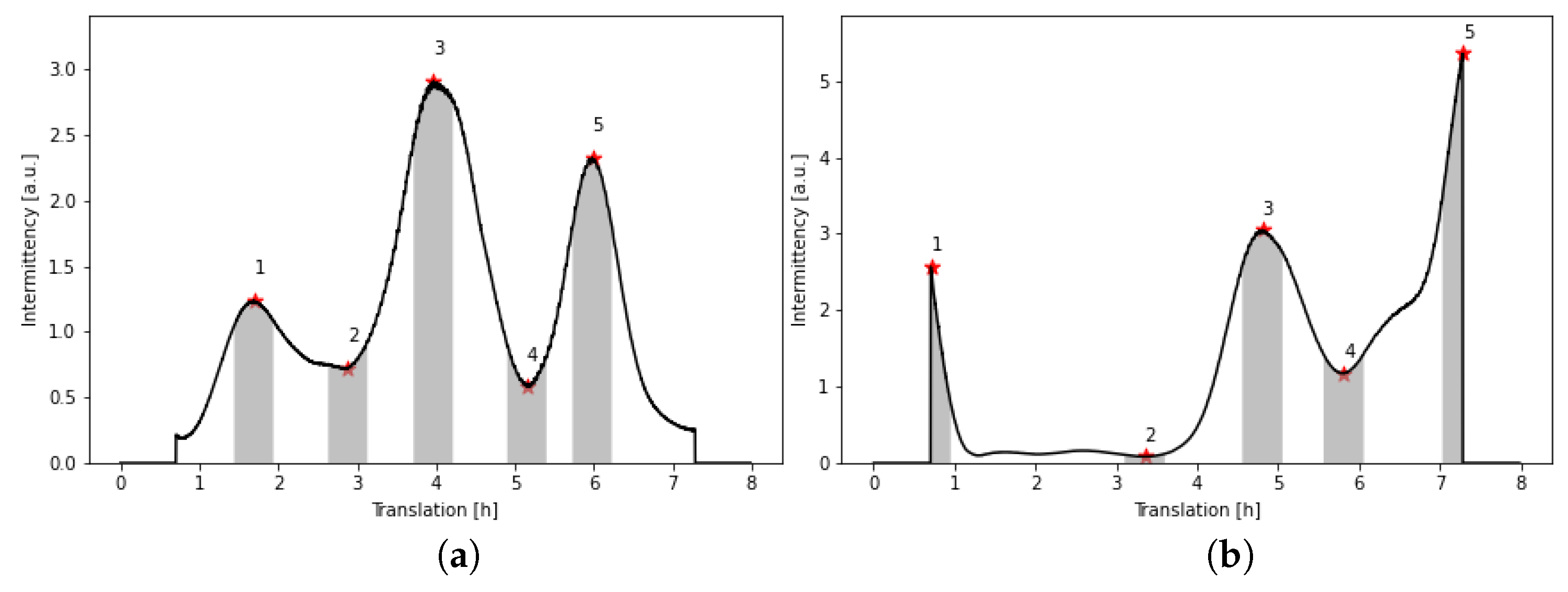
Figure 4.
Selection of time instances for analysis for observation (a) L82655, (b) L79324.
Figure 4.
Selection of time instances for analysis for observation (a) L82655, (b) L79324.
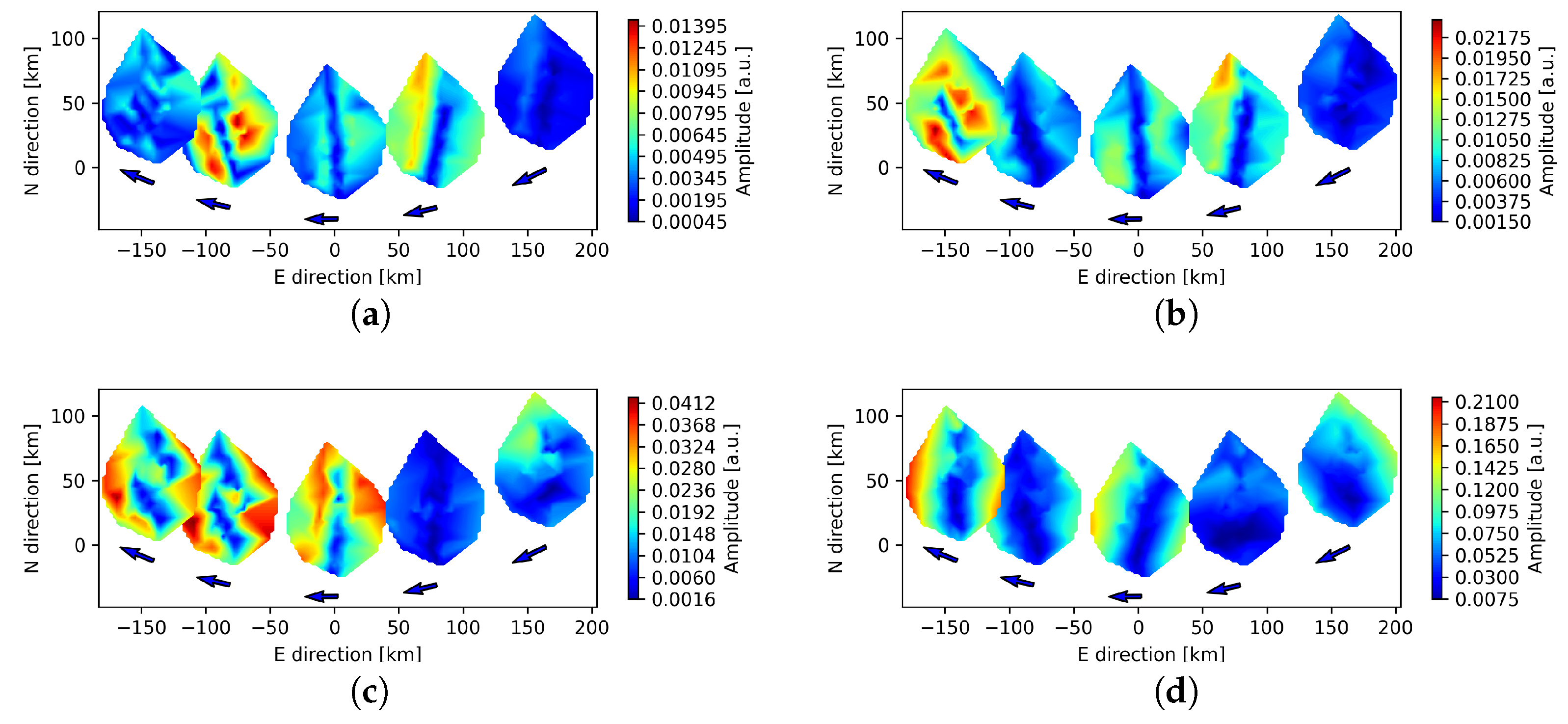
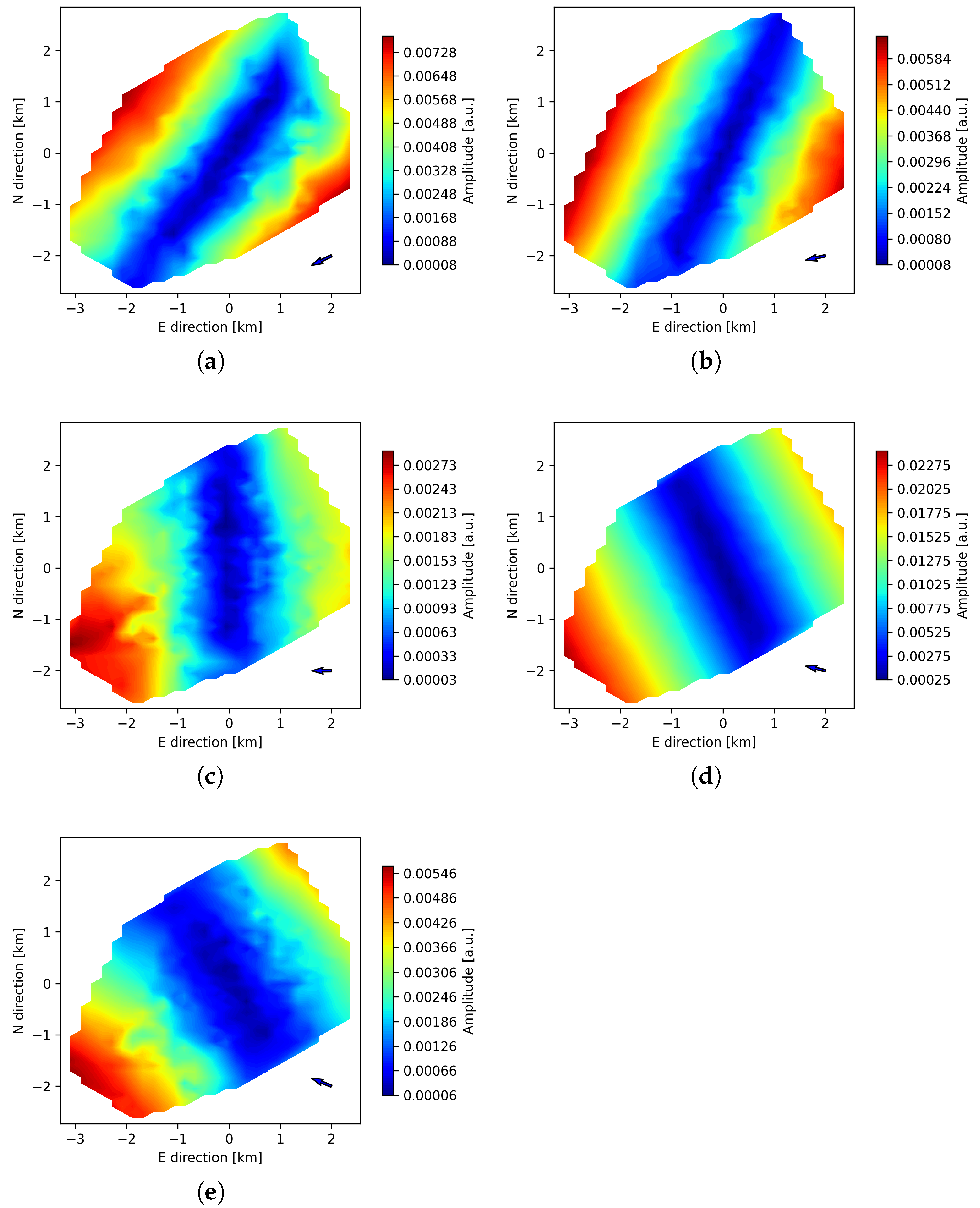
Figure 5.
Spatial distribution of amplitudes for remote stations of L82655 at 3, 4, 12 and 27 min central periods (panels (a–d), respectively). Arrows indicate the direction of LOS propagation.
Figure 5.
Spatial distribution of amplitudes for remote stations of L82655 at 3, 4, 12 and 27 min central periods (panels (a–d), respectively). Arrows indicate the direction of LOS propagation.
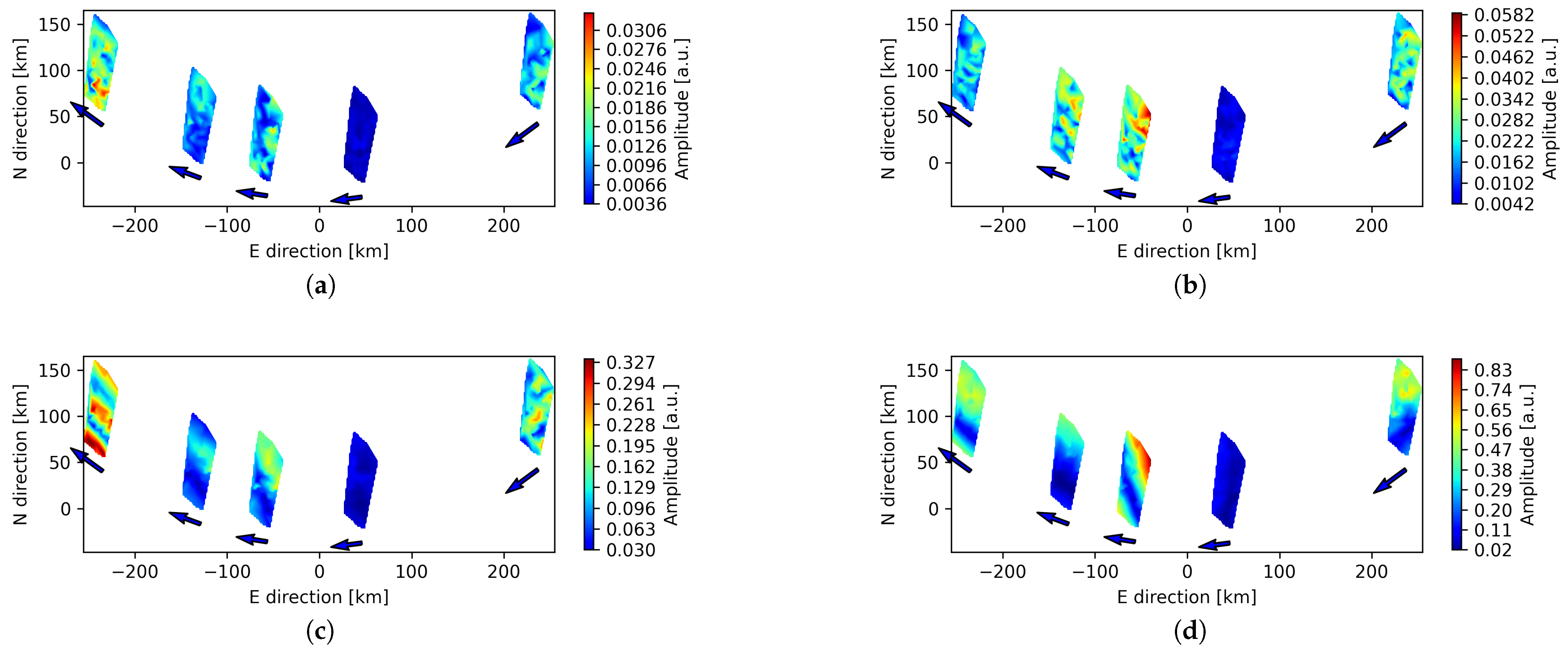
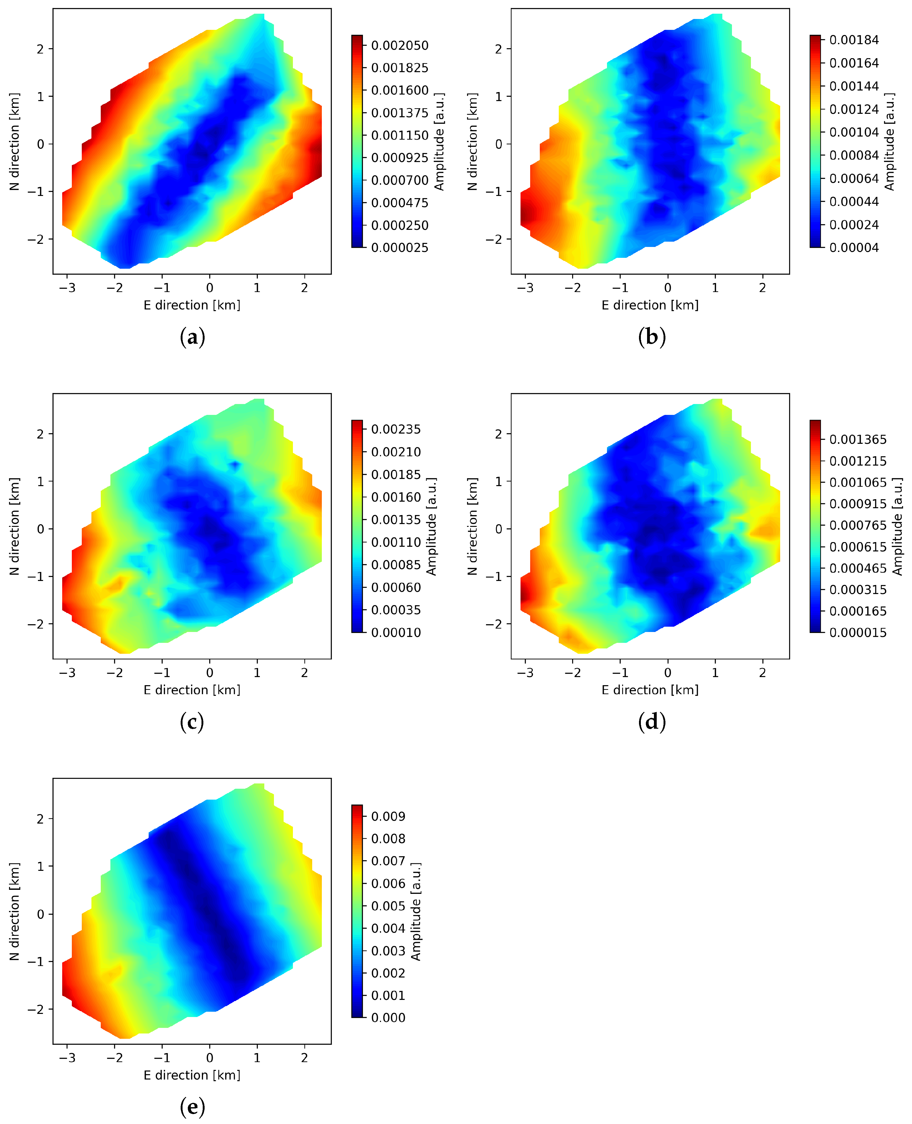
Figure 6.
Spatial distribution of amplitudes for remote stations of L79324 at 3, 4, 12 and 27 min central periods (panels (a–d), respectively). Arrows indicate the direction of LOS propagation.
Figure 6.
Spatial distribution of amplitudes for remote stations of L79324 at 3, 4, 12 and 27 min central periods (panels (a–d), respectively). Arrows indicate the direction of LOS propagation.
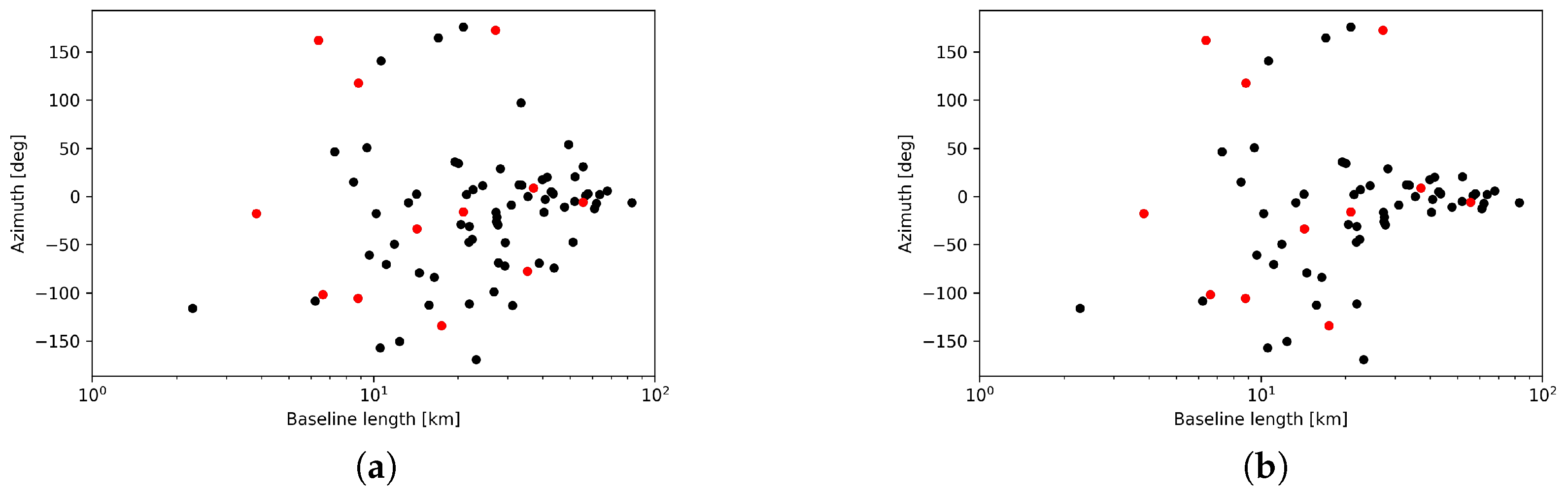
Figure 7.
Baselines’ azimuths and lengths distribution for all combinations of remote stations for (a) L82655 and (b) L79324. Red dots denote original baselines, black dots denote additional combinations.
Figure 7.
Baselines’ azimuths and lengths distribution for all combinations of remote stations for (a) L82655 and (b) L79324. Red dots denote original baselines, black dots denote additional combinations.
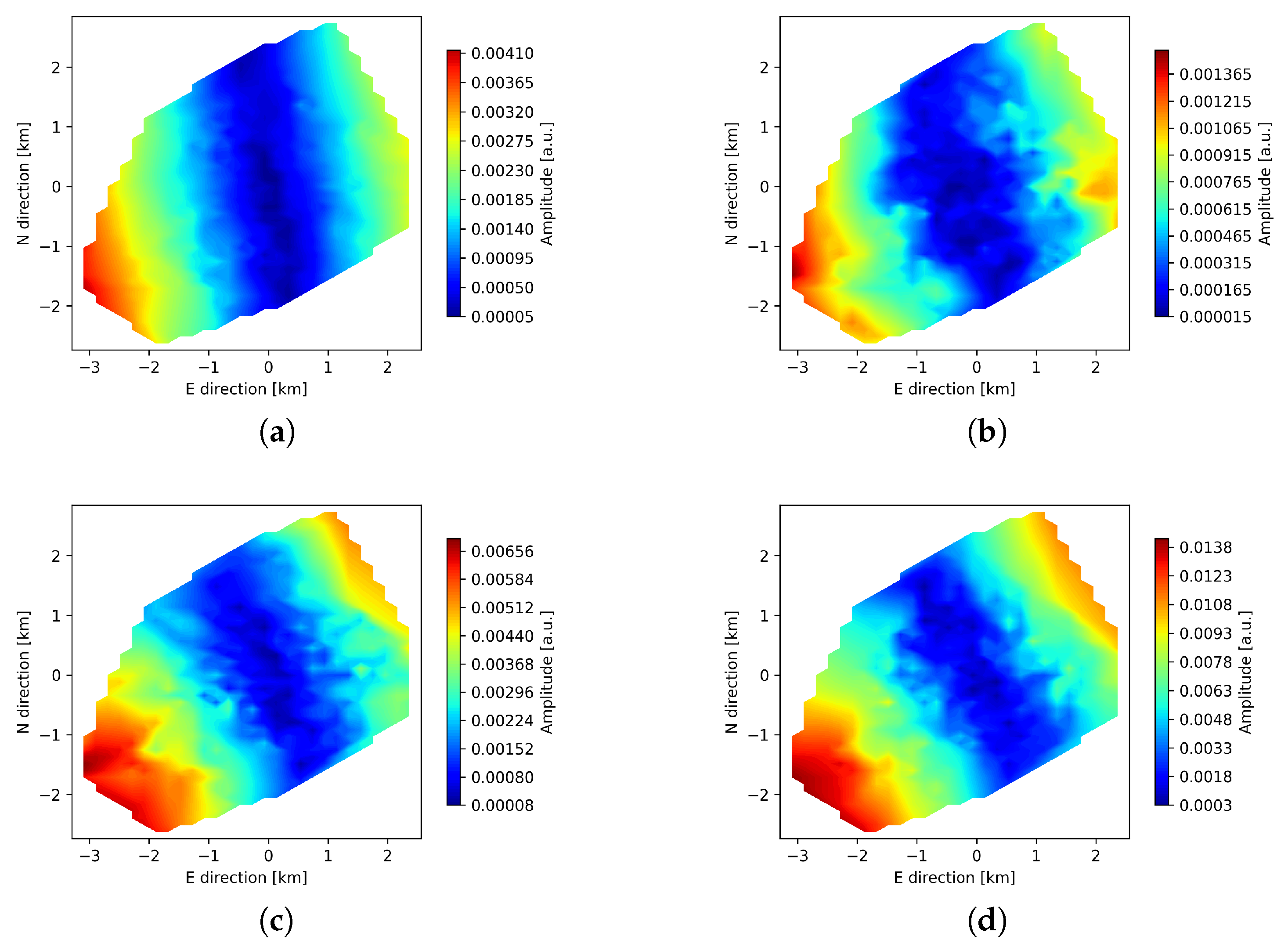
Figure 8.
Amplitudes of core stations for the peak 4 of L82655; panels (a–d) correspond to 3, 4, 12 and 27 min central periods, respectively.
Figure 8.
Amplitudes of core stations for the peak 4 of L82655; panels (a–d) correspond to 3, 4, 12 and 27 min central periods, respectively.
Figure 9.
Amplitudes of core stations for observation L82655 for peaks 1–5 of L82655 peaks set (panels (a–e)) at 4 min central period (see text).
Figure 9.
Amplitudes of core stations for observation L82655 for peaks 1–5 of L82655 peaks set (panels (a–e)) at 4 min central period (see text).
Figure 10.
Amplitudes of core stations for observation L79324 for peaks 1–5 of L82655 peaks set (panels (a–e)) at 4 min central period (see text).
Figure 10.
Amplitudes of core stations for observation L79324 for peaks 1–5 of L82655 peaks set (panels (a–e)) at 4 min central period (see text).
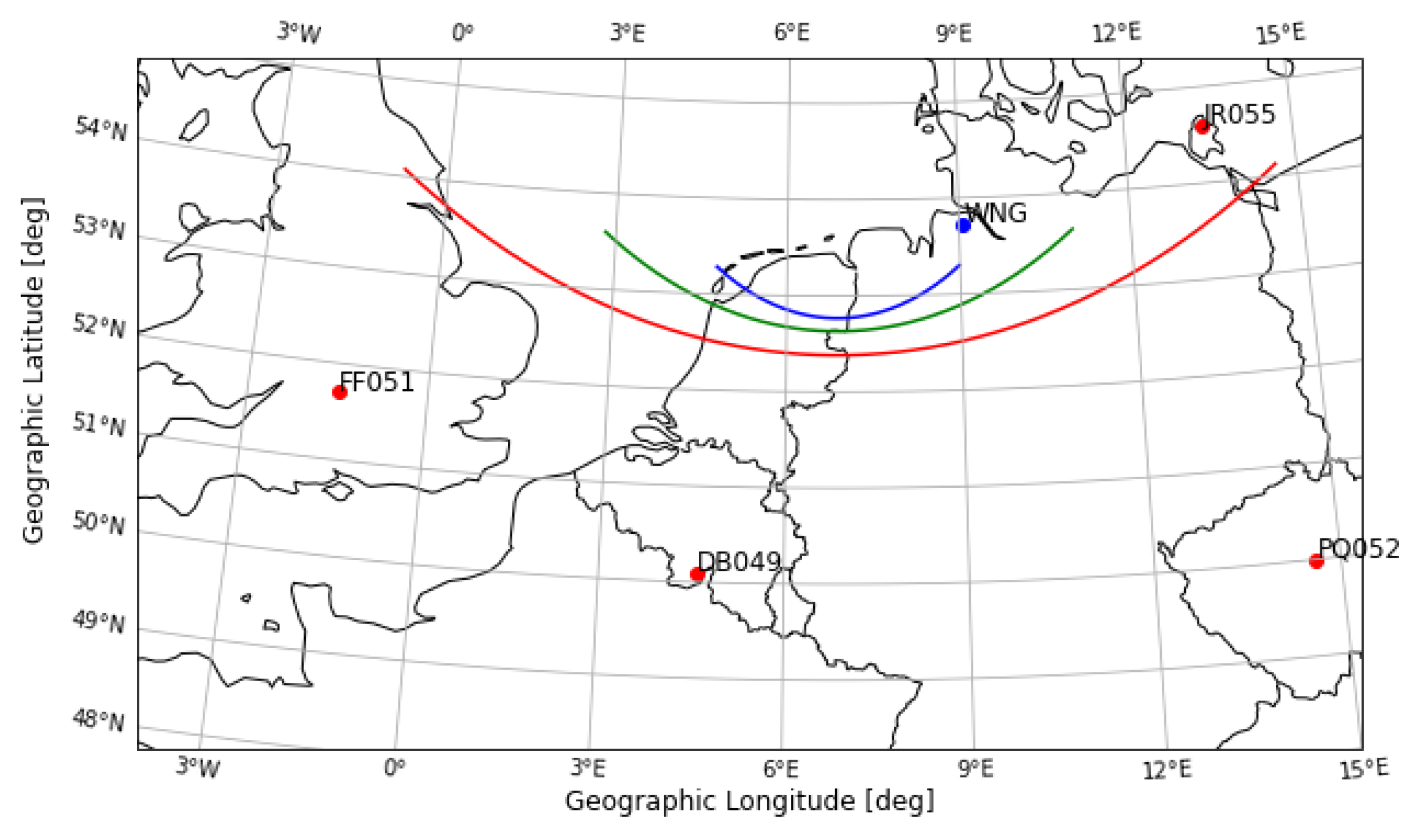
Figure 11.
Location of LOFAR pierce points (at 200, 400 and 800 km altitude marked with blue, green and red line, respectively) relative to the observatories used in the analysis. Red dots: stations that serve as a source of ionospheric plasma drift data; geomagnetic field data were obtained from the stations WNG and DOU (marked as DB049).
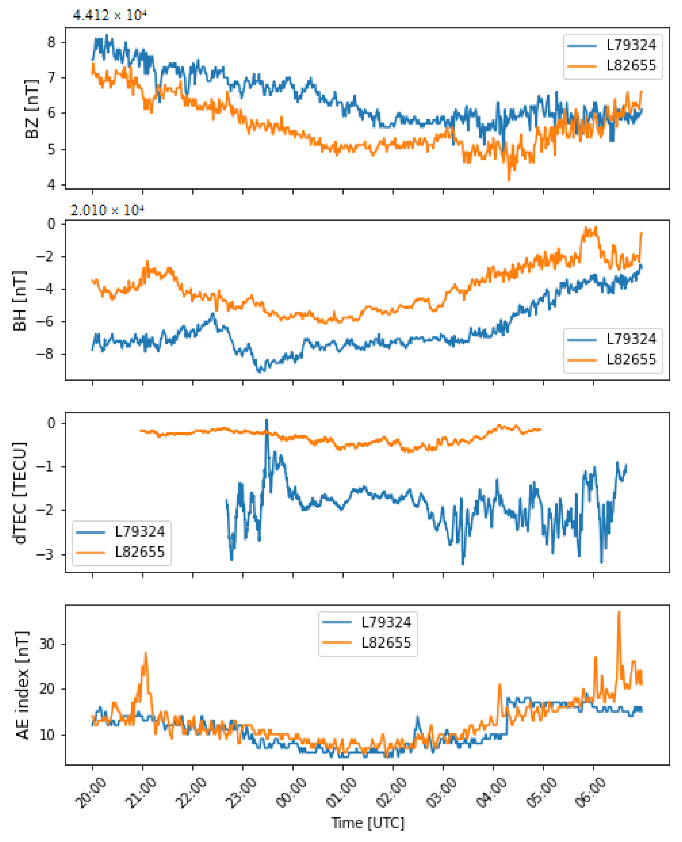
Figure 12.
Geomagnetic field for DOU station and LOFAR dTEC signal for both observations. From top to bottom: vertical component of geomagnetic field (BZ), horizontal component of geomagnetic field (BH), sum of dTEC values of LOFAR baselines, auroral electrojet index value (AE).
Figure 12.
Geomagnetic field for DOU station and LOFAR dTEC signal for both observations. From top to bottom: vertical component of geomagnetic field (BZ), horizontal component of geomagnetic field (BH), sum of dTEC values of LOFAR baselines, auroral electrojet index value (AE).
Figure 13.
Changes of the geomagnetic field with respect to the mean value of the observation timespan; (a) L82655, DOU observatory; (b) L82655, WNG observatory; (c) L79324, DOU observatory; (d) L79324, WNG observatory. Color scale shows time from the start of the observations.
Figure 13.
Changes of the geomagnetic field with respect to the mean value of the observation timespan; (a) L82655, DOU observatory; (b) L82655, WNG observatory; (c) L79324, DOU observatory; (d) L79324, WNG observatory. Color scale shows time from the start of the observations.
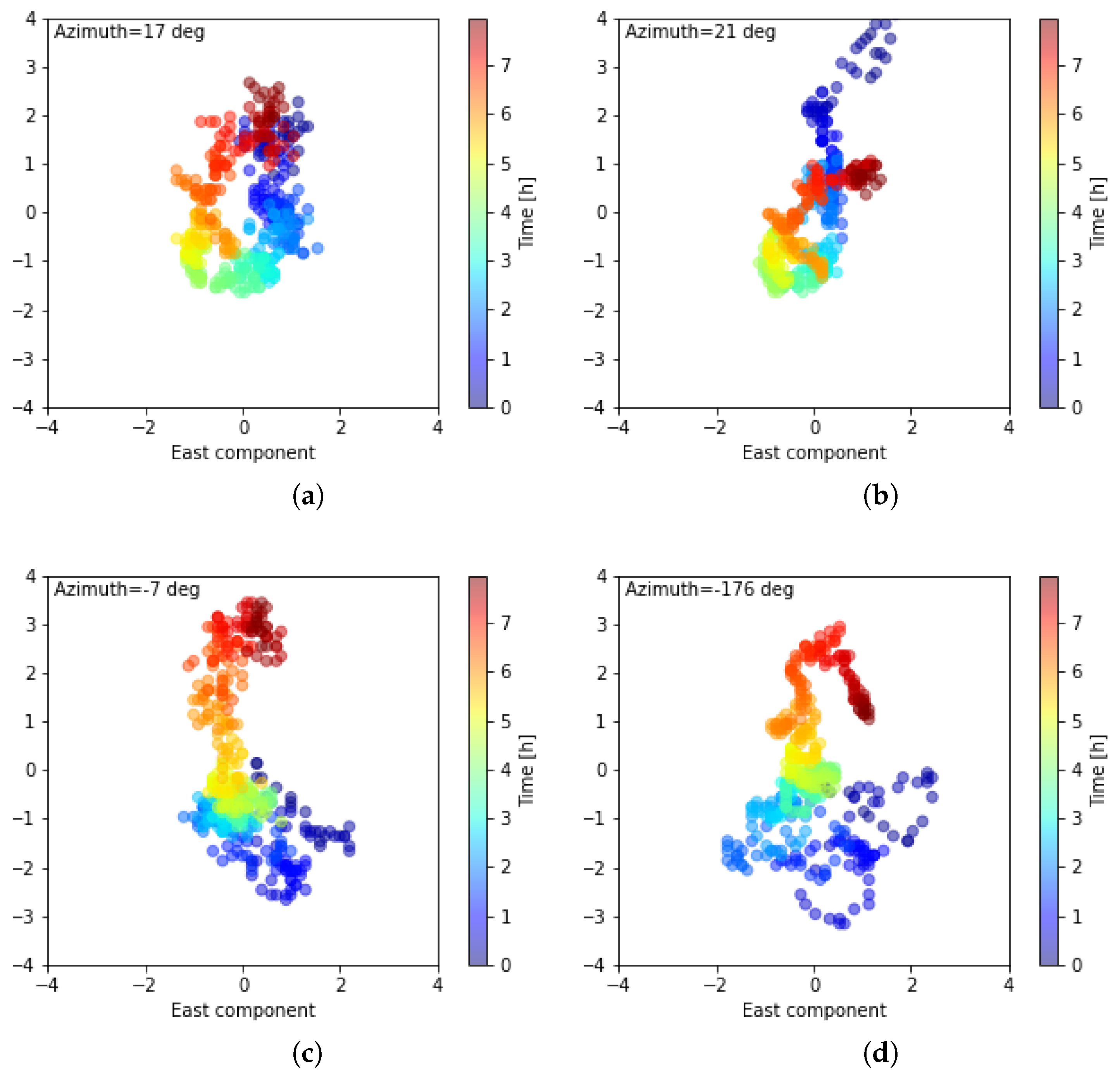
Figure 14.
LOFAR amplitudes for 3 min central period for (a) L82655 and (b) L79324. Color scale shows time from the start of observation. Black arrows indicate the dominant directions calculated from Principal Components Analysis (PCA), with the azimuth value provided for the direction explaining majority of variance.
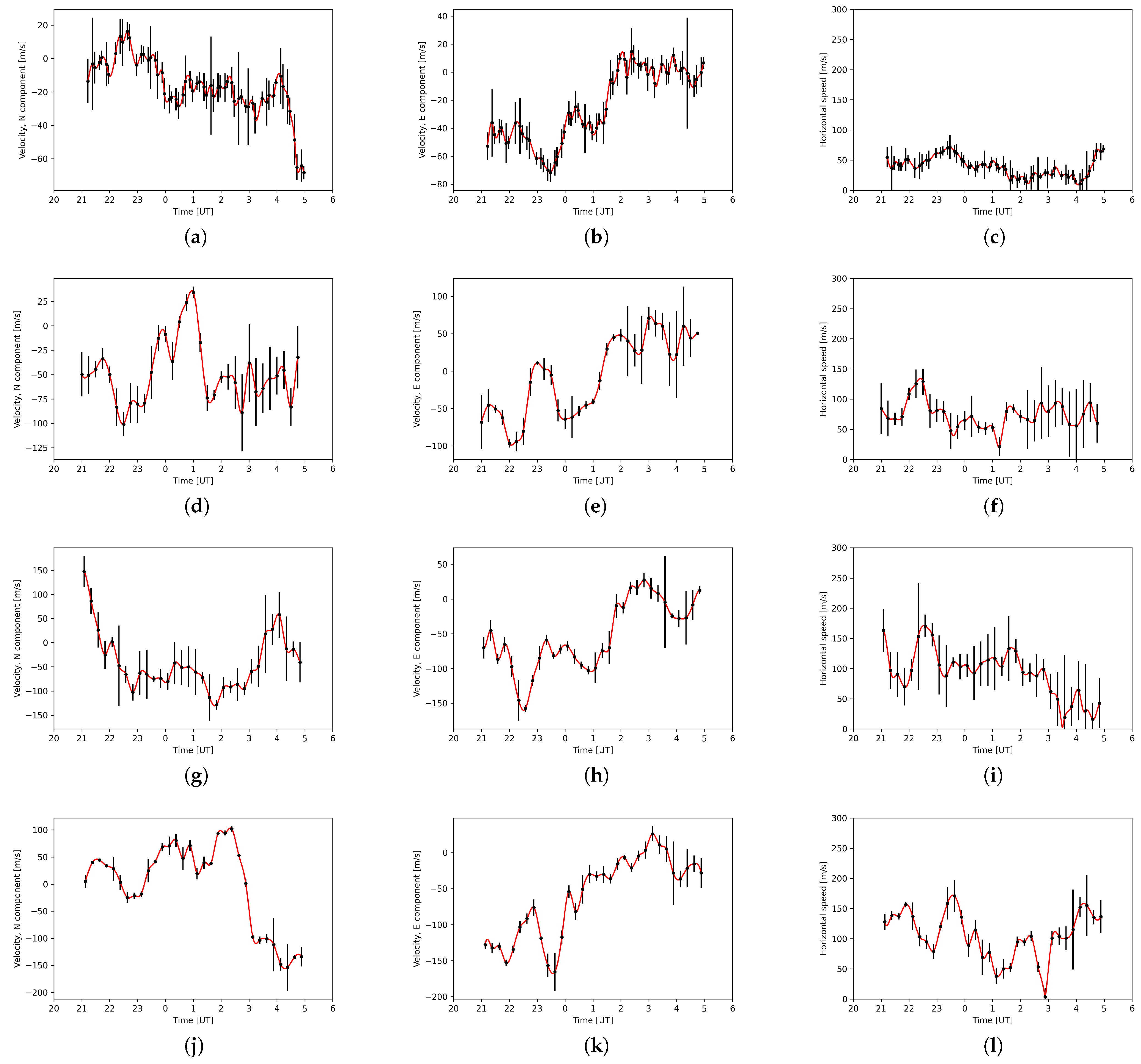
Figure 15.
F layer plasma drift velocity data for L82655 with interpolated values (red line) for the North component, East component and horizontal speed of (a–c) DB, (d–f) JR, (g–i) PQ and (j–l) FF stations, respectively.
Figure 15.
F layer plasma drift velocity data for L82655 with interpolated values (red line) for the North component, East component and horizontal speed of (a–c) DB, (d–f) JR, (g–i) PQ and (j–l) FF stations, respectively.
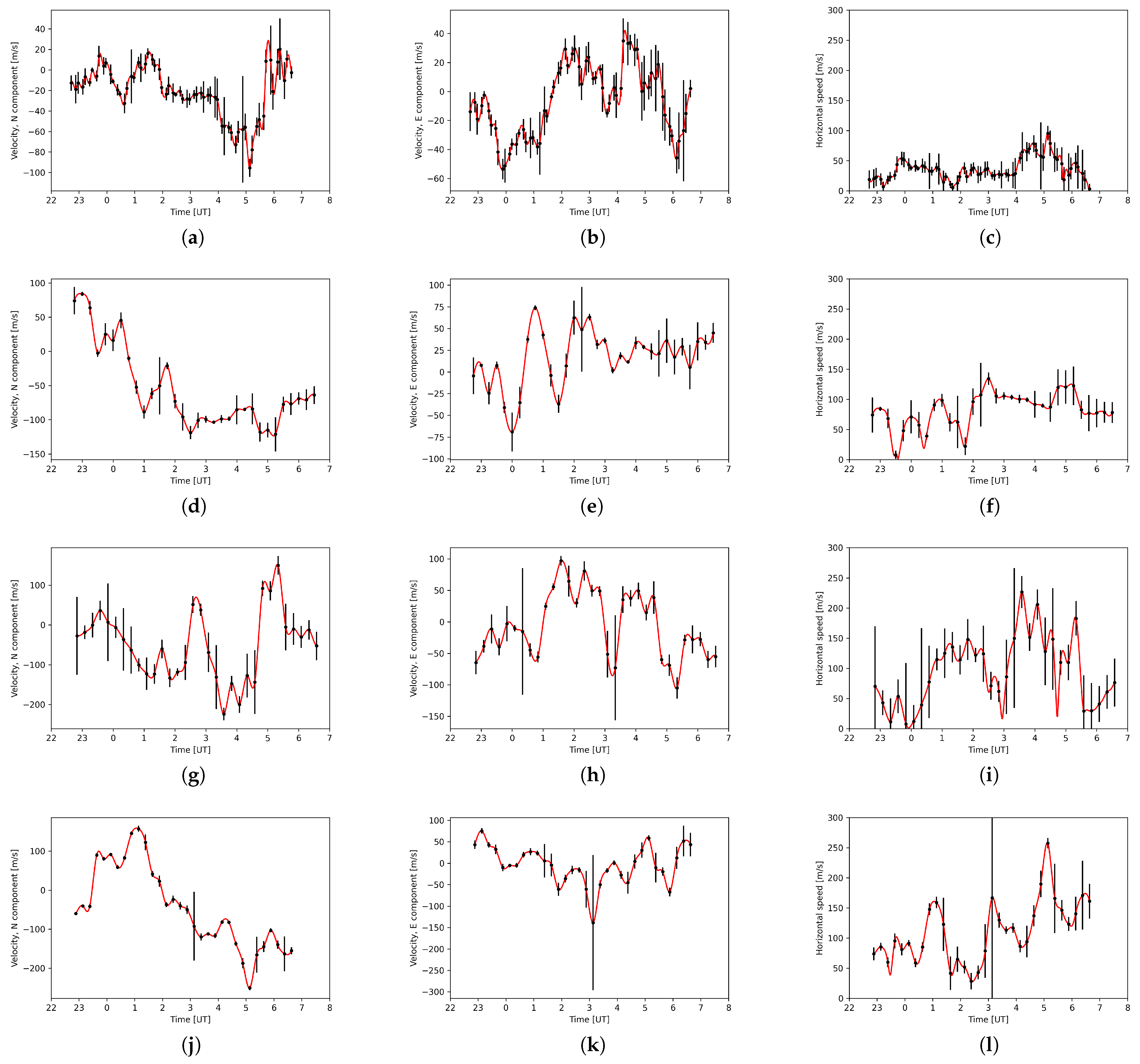
Figure 16.
F layer plasma drift velocity data for L79324 with interpolated values (red line) for the North component, East component and horizontal speed of (a–c) DB, (d–f) JR, (g–i) PQ and (j–l) FF stations, respectively.
Figure 16.
F layer plasma drift velocity data for L79324 with interpolated values (red line) for the North component, East component and horizontal speed of (a–c) DB, (d–f) JR, (g–i) PQ and (j–l) FF stations, respectively.
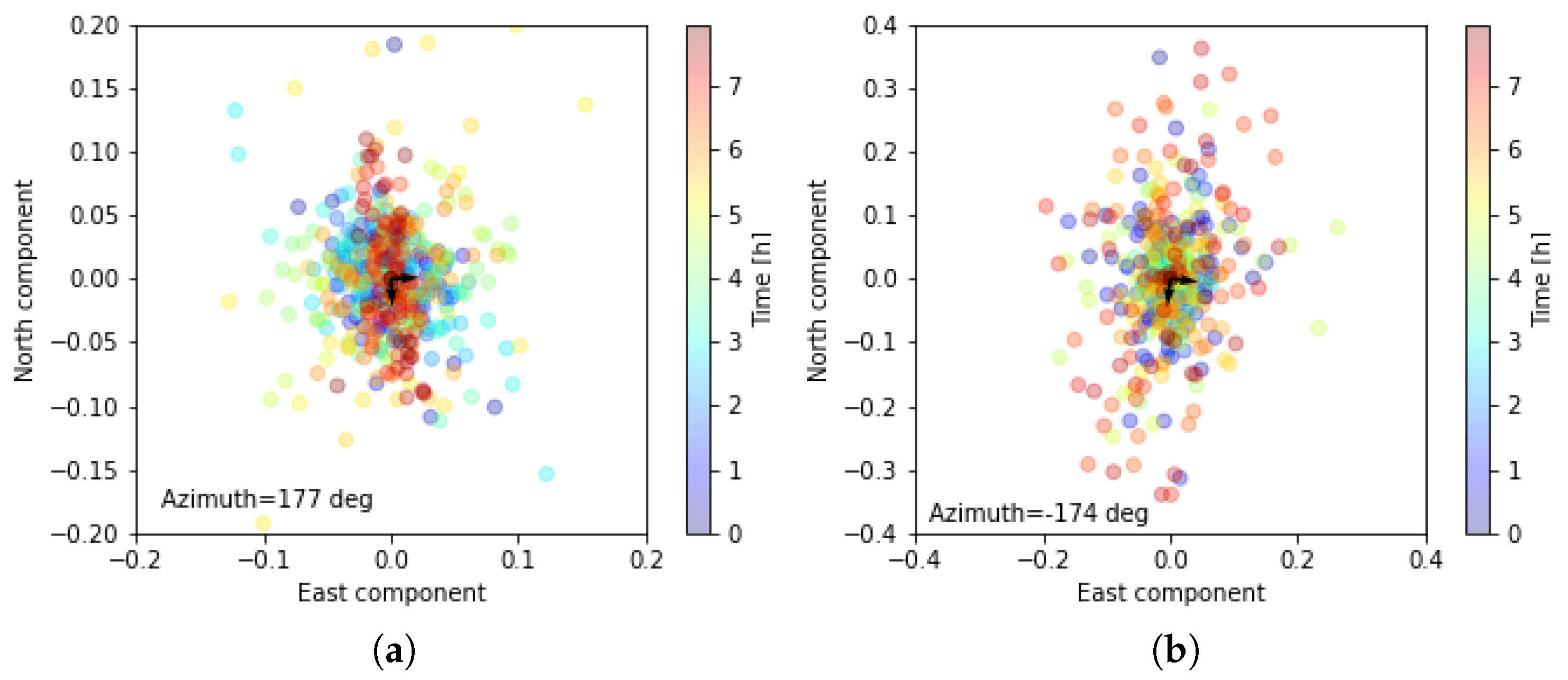
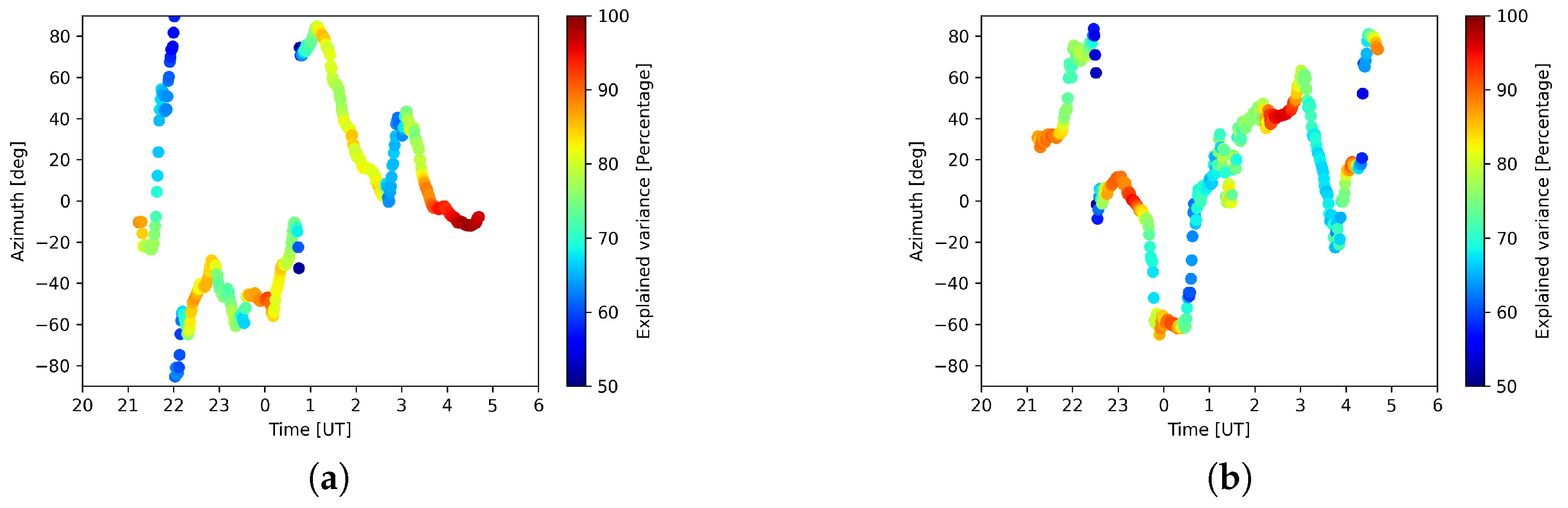
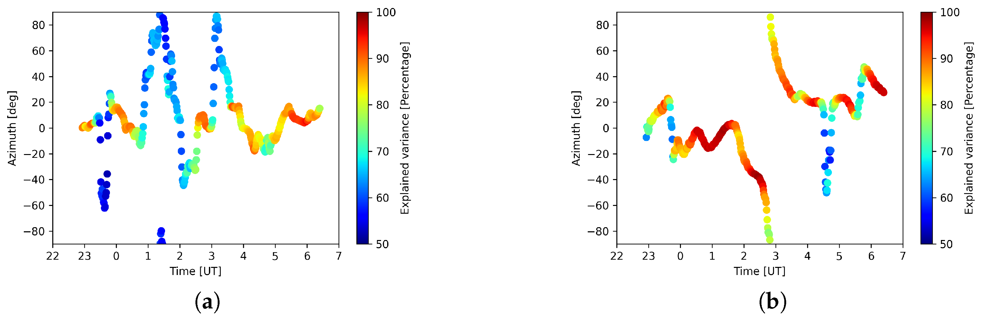
Figure 17.
L82655 PCA azimuths for principal components (a) at 3 min central period and (b) at 12 min central period. Color scale shows percentage of signal’s variance explained by the components.
Figure 17.
L82655 PCA azimuths for principal components (a) at 3 min central period and (b) at 12 min central period. Color scale shows percentage of signal’s variance explained by the components.
Figure 18.
L79324 PCA azimuths for principal components (a) at 3 min central period and (b) at 12 min central period. Color scale shows percentage of signal’s variance explained by the components.
Figure 18.
L79324 PCA azimuths for principal components (a) at 3 min central period and (b) at 12 min central period. Color scale shows percentage of signal’s variance explained by the components.
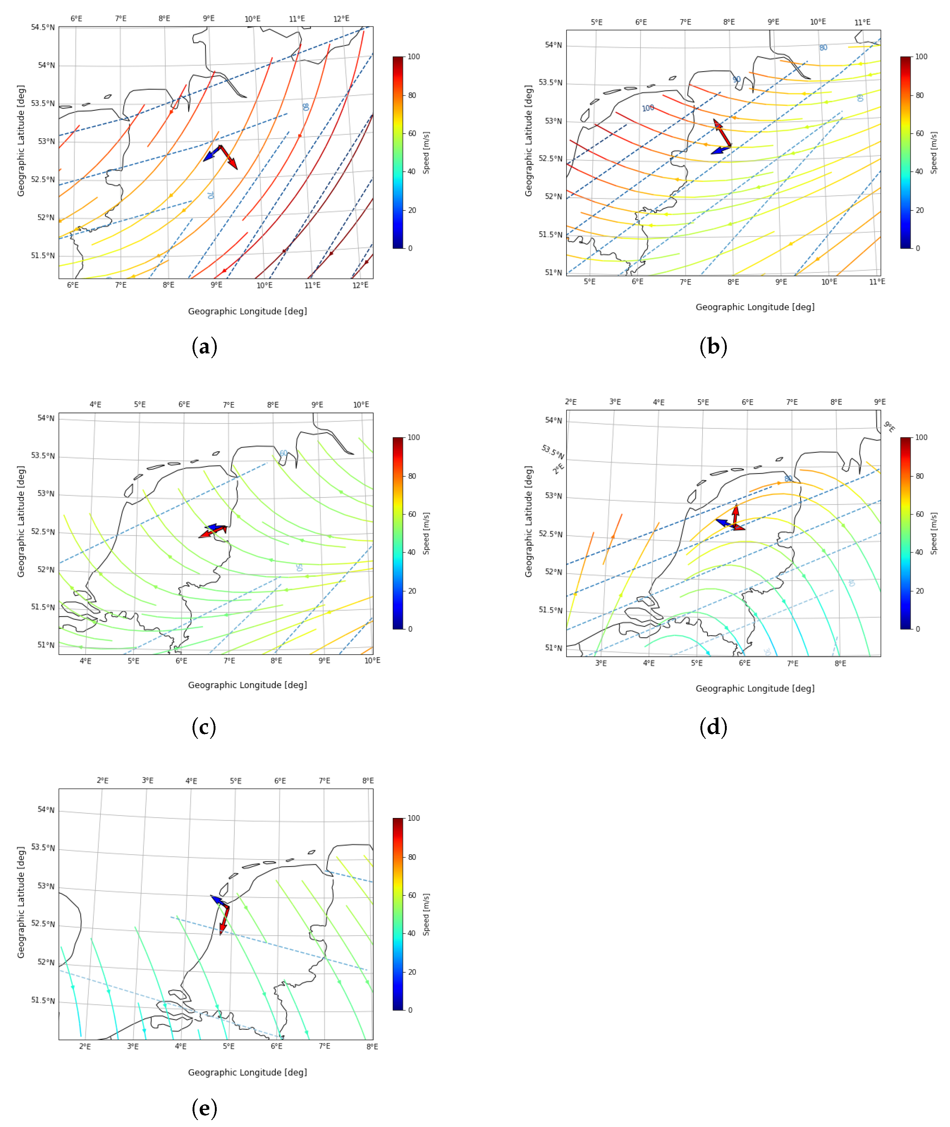
Figure 19.
Spatial distribution of plasma drift velocity for the peaks 1-5 (panels (a–e), respectively) of L82655. Streamlines show plasma velocity vectors based on four digisondes (outside the map’s scope), blue lines: isolines of horizontal speed. Blue arrow: LOS propagation direction, red arrows: fitted directions of the disturbances based on 4 min central period wavelet coefficients, scaled by the percentage of explained variance.
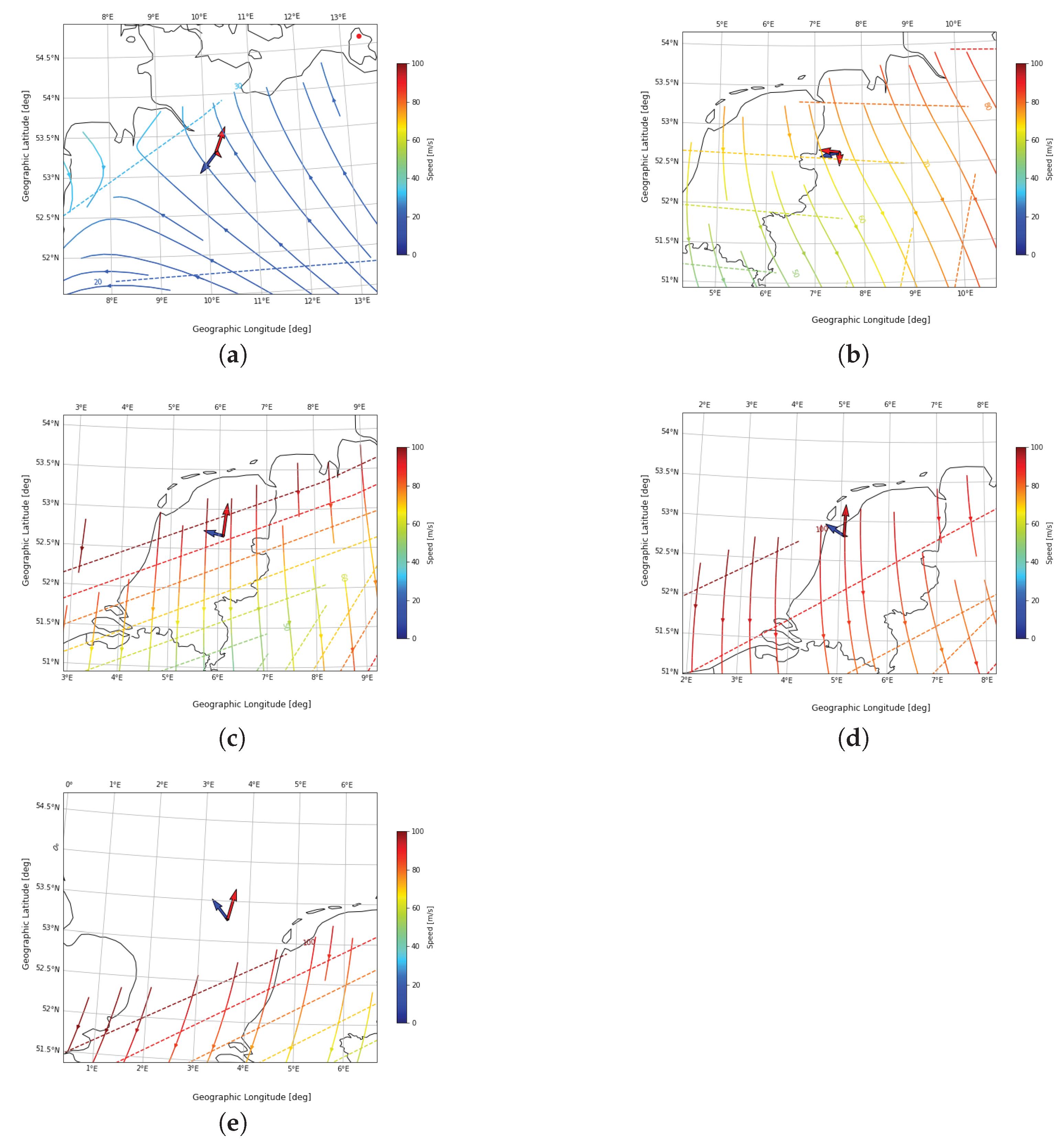
Figure 20.
Spatial distribution of plasma drift velocity for the peaks 1-5 (panels (a–e), respectively) of L79324. Streamlines show plasma velocity vectors based on four digisondes (outside the map’s scope), blue lines: isolines of horizontal speed. Blue arrow: LOS propagation direction, red arrows: fitted directions of the disturbances based on 4 minutes central period wavelet coefficients, scaled by the percentage of explained variance.
Table 1.
UT time of the peaks for the selected intervals.
Table 1.
UT time of the peaks for the selected intervals.
| Peak | L82655 | L79324 |
|---|
| 1 | 22:40 | 23:23 |
| 2 | 23:51 | 02:02 |
| 3 | 00:56 | 03:29 |
| 4 | 02:07 | 04:30 |
| 5 | 02:57 | 05:58 |


