1. Introduction
In recent years, road collapses, which are usually caused by the development of cavities in road subgrades, have frequently occurred. They may affect traffic or cause casualties and serious property losses. Therefore, it is necessary to dynamically monitor road subgrade diseases.
Due to the GPR advantages of rapidness, high resolution, and nondestructiveness, it is widely used in road layer thickness measurements [
1,
2,
3], cavity and crack detection [
4,
5,
6], asphalt layer quality assessment [
7,
8,
9], the detection of moisture and water content changes [
10,
11,
12]. However, most of these studies were performed based on 2D GPR detection, which has the problems of false detection and missing detection, as the survey lines were sparse and the acquired information was inadequate. Using 3D GPR for data acquisition and imaging can well reveal underground structures [
13]. Full-resolution 3D GPR imaging can be realized by arranging 2D grids with a line spacing of less than one-quarter of the wavelength [
14,
15,
16]. Unfortunately, the main limitation of this method is that it is time-consuming. As a result, it is hard to perform the full-coverage detection of roads without affecting traffic. With the appearance of multi-channel array antenna 3D GPR, the detection efficiency and accuracy of the combination of survey lines have greatly been improved, making this method suitable for the full-coverage detection of roads [
17].
Furthermore, road subgrades have the characteristics of dynamic change under the action of vehicle rolling and underground engineering. Therefore, it is urgent to perform short-interval periodic detection on roads based on 3D GPR so as to repair the areas where road disasters may occur. At present, the application of GPR in the monitoring field is mainly based on underground hydrological process monitoring [
18,
19,
20,
21,
22,
23], pollutant monitoring [
24,
25], gas migration monitoring [
26], road stripping monitoring [
27], underground facility monitoring [
28], and railway monitoring [
29].
Compared with the existing studies mentioned above, the full-coverage monitoring of roads has the characteristics of long-term, less-known information, dense survey lines, strong interference, and other uncertain factors. In addition, the differences between time-lapse GPR data are weak, and some of them are caused by nonunderground changes, which greatly increase the difficulty of data interpretation. Hence, it is particularly important to study data processing and interpretation methods. At present, the research on time-lapse GPR data processing mainly focuses on amplitude normalization, time zero correction, spatial position matching, four-dimensional grid interpolation, sampling rate fluctuation correction, and abnormal amplitude correction [
23,
28,
30,
31,
32]. Furthermore, the interpretation methods of time-lapse data include difference [
24,
32], attribute analysis [
20,
23], K-means clustering [
28], amplitude analysis [
33], and electromagnetic wave velocity analysis [
22,
34]. In short, eliminating the differences caused by nonunderground changes and searching the changed areas in time-lapse GPR data are key problems of data processing and interpretation.
In this paper, we present a road subgrade monitoring technology based on time-lapse full-coverage (TLFC) 3D GPR. It relies on eliminating the differences caused by nonunderground changes and analyzing the differences in the attributes between time-lapse data. Through the design of a full-coverage road monitoring experiment, TLFC 3D GPR data were acquired. Then, time zero consistency correction, 3D data combination, spatial position matching, and interpretation based on a time-lapse attribute were performed on the acquired data. The 3D imaging quality of the TLFC 3D GPR data to underground space was significantly improved, and the changing area was highlighted. Finally, we summarized the dynamic changing rule of subgrade and its causes are analyzed.
2. Experimental Design and Data Acquisition
2.1. Experimental Area
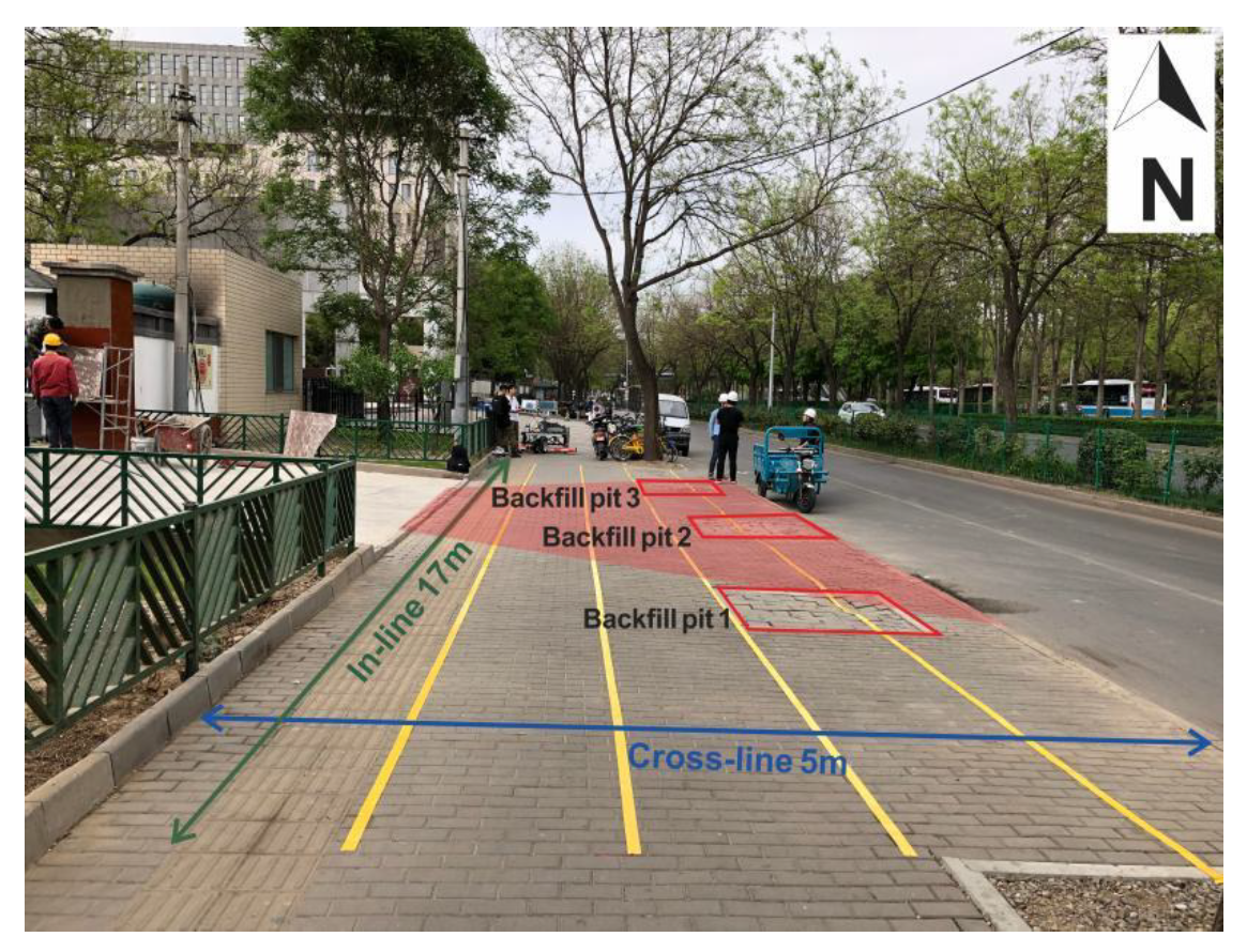
We designed the periodic detection experiment on a sidewalk whose subgrade may change. This area was rolled by engineering vehicles outside a subway construction site, and it covers an area of 85 (17 × 5) m
2 and has three backfill pits, as shown in
Figure 1. The red shaded area faces the gate of the construction site and belongs to the key rolling area.
2.2. TLFC 3D GPR Data Acquisition
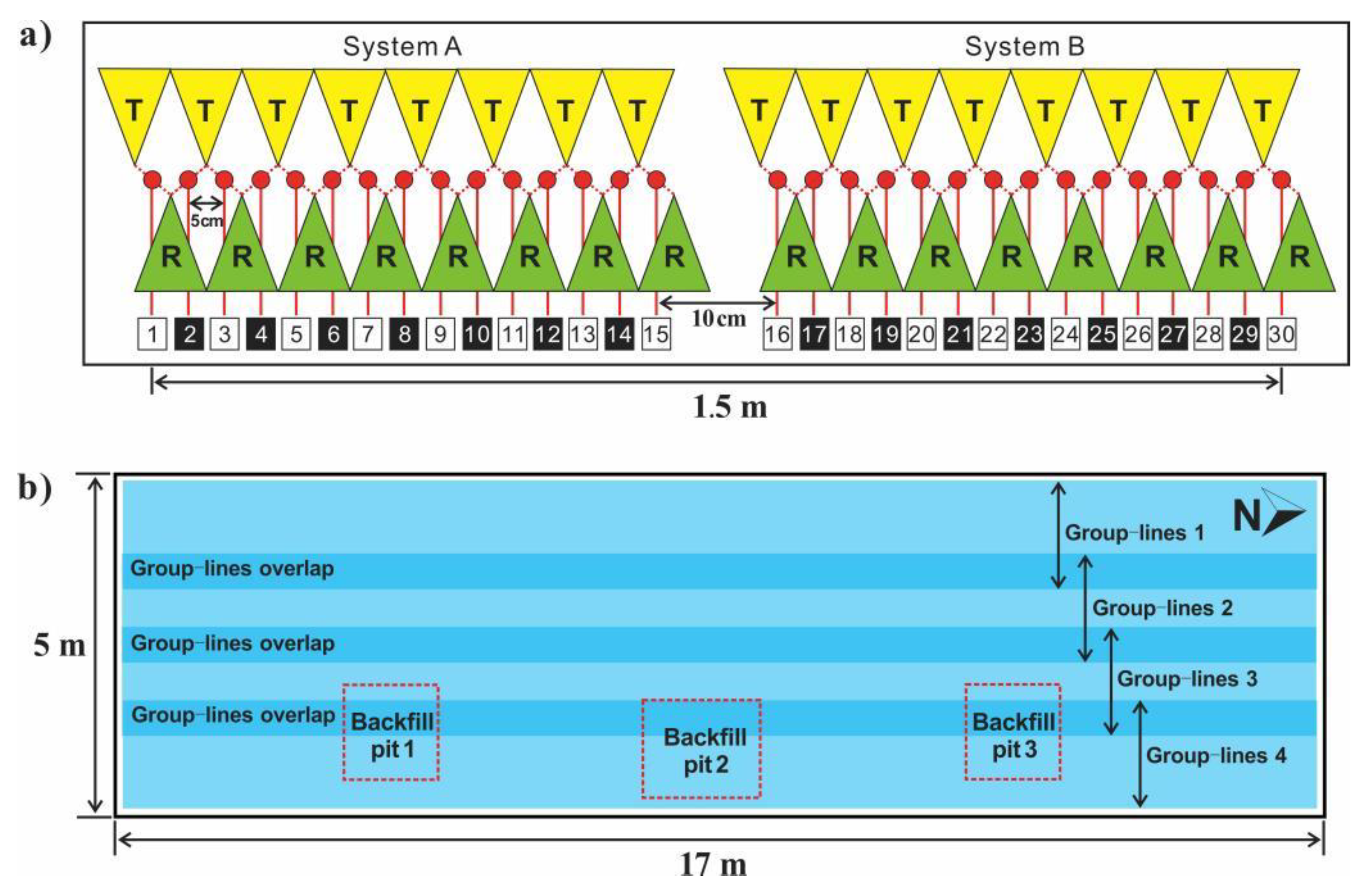
Mobyscan-V 3D GPR, which was produced by DECOD of Singapore, was used in this monitoring experiment. A 2-GHz high-frequency array antenna that includes 16 pairs of receiving and transmitting antennas was selected, forming 30 data channels with a spacing of 5 cm (
Figure 2a). Single group lines could cover a width of 1.5 m, and there was a 10 cm gap between System A and System B. By designing four group lines on the sidewalk, full-coverage of the rolling area was realized. There were 11 overlapping channels between the adjacent group lines, which provided a guarantee for the accurate combination of different group lines (
Figure 2b). Furthermore, due to the frequent passing of engineering vehicles on the sidewalks, we selected a short detection time interval, ranging from 8 to 14 days, to clearly show the change process of the subgrade.
Table 1 shows the acquisition parameters.
3. Data Processing and Imaging
Reasonable data processing is crucial for ensuring the reliability of detection results, and it greatly improves the imaging quality of underground 3D spaces. The key problems of TLFC 3D GPR data processing include two aspects. First, for the full-coverage 3D GPR data acquired on the same date, we mainly solve the inconsistency of time zero and the dislocation of multiple group lines. Second, for the time-lapse data acquired on different dates, the main purpose is to eliminate the differences between survey line positions and accurately obtain the repeated parts. Therefore, the designed processing scheme for monitoring experimental data includes (1) preprocessing, (2) time zero consistency correction, (3) 3D data combination of the adjacent group lines, and (4) spatial position matching.
3.1. Preprocessing
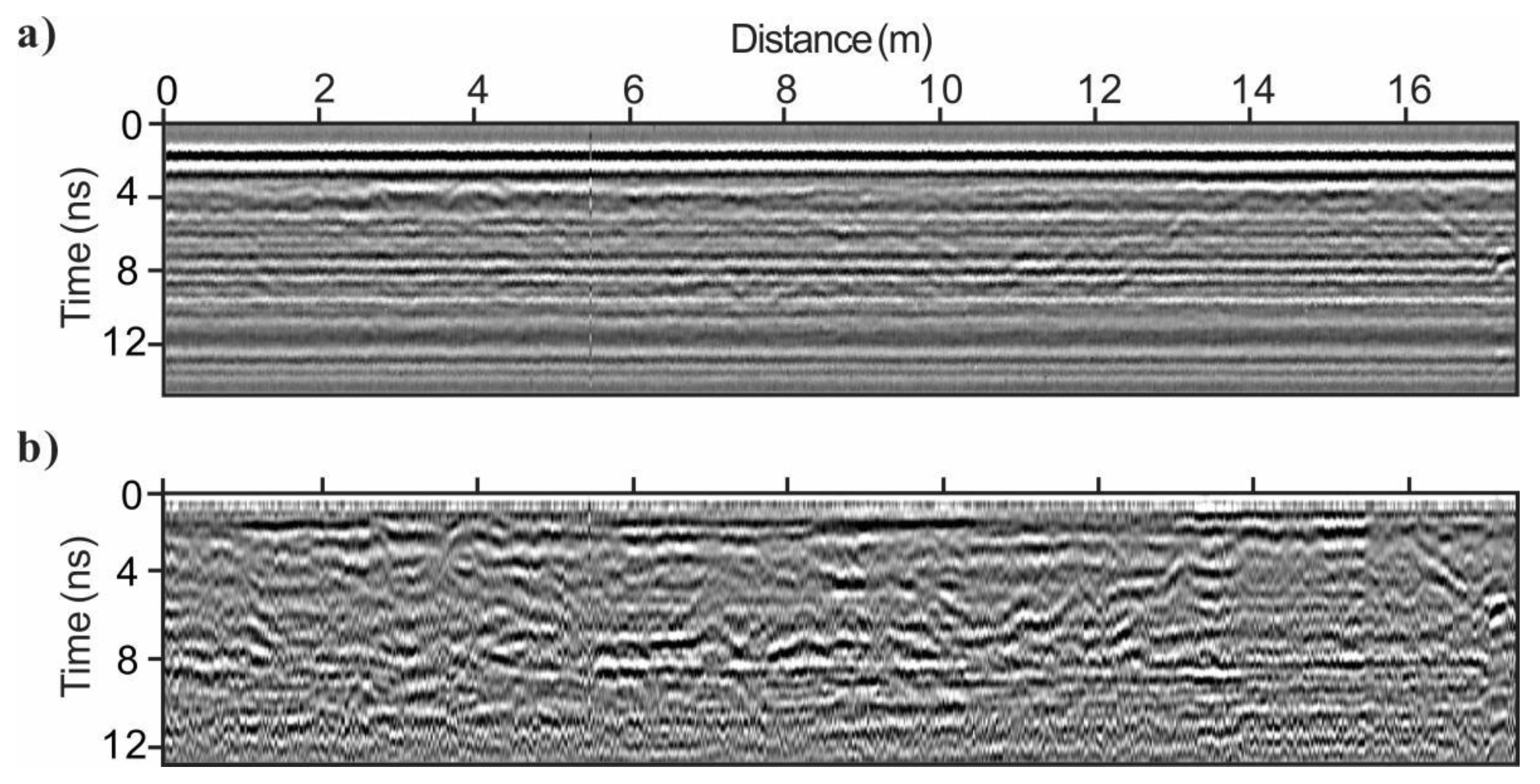
Due to the electromagnetic wave characteristics of high frequency and short wavelength, classic processing methods should be selected to ensure the authenticity of reflected waves. Using the ReflexW software, time zero correction, background removal, exponential gain, and bandpass filtering (using a Butterworth bandpass filter with a passband of 400–1500 MHz) are mainly performed. The GPR data profiles before and after preprocessing are shown in
Figure 3a,b. The clutter in the processed data was well eliminated, and the events of the reflected wave from the underground interface became clearer.
3.2. Time Zero Consistency Correction and Imaging
After preprocessing, we noticed that the events were rough and fuzzy, as shown in
Figure 3b. This is due to the shaking of the antenna during movement and the system stability fluctuation. This problem introduces false anomalies into 3D GPR data, especially in horizontal slices, which greatly reduces the reliability of interpretation results. To realize high-quality imaging of the underground 3D structure and provide interpretation guarantees, the time zero needed to be corrected to the same position before the preprocessing process. Since the ground direct wave has a good correlation and belongs to strong reflection, the most relevant position on the time axis could be found by calculating the correlation sequence of each trace’s direct wave. The time zero correction includes the following three procedures.
- (1)
Determining the reference trace
The reference trace credibility directly determines the accuracy of time zero position normalization and correction. Hence, the one trace with a known direct wave travel time is selected as a reference trace, and the other traces are corrected.
- (2)
Correction time calculation
The cross-correlation sequence of the direct wave between
and
is calculated according to Equation 1, and the correction amount
is obtained when
is maximum.
- (3)
Correction
If , there is no need to move the trace to be corrected. Otherwise ( or ), the trace to be corrected needs to move sampling points, positive or negative, along the time axis.
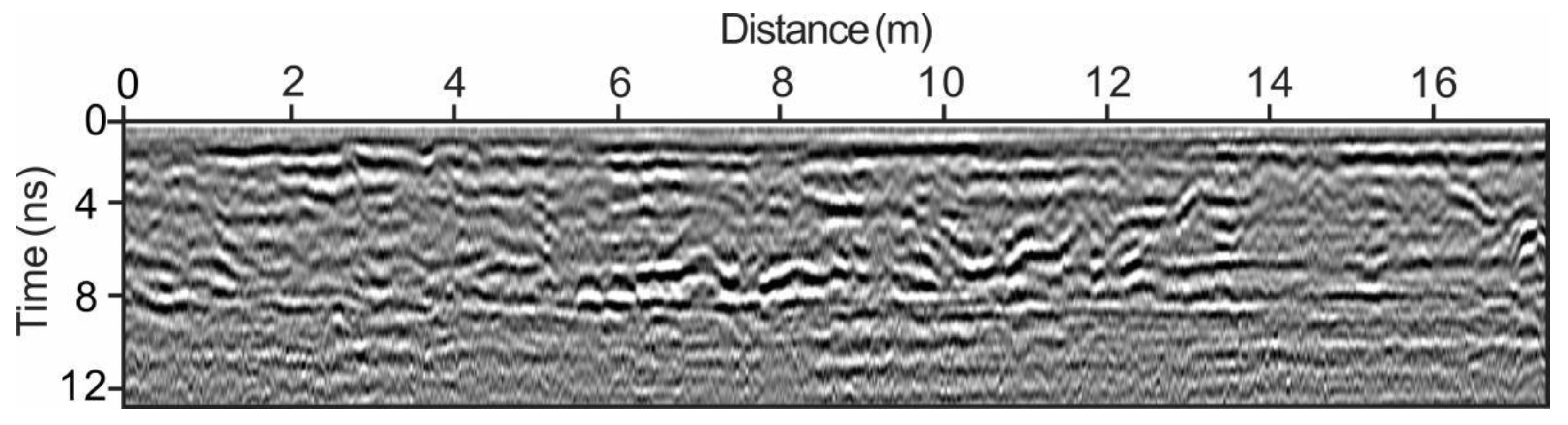
The time zero consistency correction could be completed by performing the above method so that all the traces could be corrected. In the inline profile, after the time zero correction and preprocessing steps, the jitter interference on both sides of the events was eliminated. Also, the imaging quality was greatly improved, as shown in
Figure 4.
3.3. 3D Data Combination and Imaging
The data interpretation accuracy could be significantly improved by using multiple parallel-group lines to perform full-coverage detection of roads, especially when abnormalities appear at the edge of group lines.
In this experiment, due to the location, differences among the adjacent group lines in the inline direction exist. If the adjacent group lines are directly combined, imaging dislocation occurs. As shown in the yellow marked-area in
Figure 5a, the two backfill pit areas in the horizontal slice are misplaced. Therefore, the 3D GPR data combination algorithm that is based on cross-correlation was studied. This algorithm includes three aspects as follows.
- (1)
Determining the reference lines from the overlapping area
Select the profile of one group lines in the overlapping area as a reference profile. Then, the profile corresponding to the position in the other group lines is the profile to be spliced.
- (2)
Calculating the relative offset of different group lines
Calculate the correlation coefficient of all the traces between the profile to be spliced and the reference profile according to Equation (2).
where
and
are the trace numbers,
is the number of sampling points of each trace, and
and
denotes the trace of the reference profile and the profile to be spliced, respectively. When the maximum value of
is obtained, it is considered that the trace
in
corresponds to the same position of the trace
in
, and the trace number of
and
are recorded as
and
, respectively. Subtract and average the trace numbers corresponding to the same position according to Equation (3) to obtain the relative offset.
- (3)
3D data volume combination and imaging
When , data combination can be performed without moving the profiles. When or , the profile is moved to be spliced along with the inline positive or negative direction by traces. Then, the data is combined.
The horizontal slice after the accurate combination of the adjacent group lines is shown in
Figure 5b. The misplaced backfill pits were restored to the rectangular and the accurate 3D imaging of the underground space was realized. This shows that the proposed data combination algorithm in this paper is effective and accurate when there is enough overlapping data between adjacent group lines.
3.4. Spatial Location Matching
In large-area road time-lapse monitoring, it is hard to ensure the complete consistency of survey line positions. The location differences between the TLFC 3D GPR data caused the reflection from the same underground object to appear at different positions in the time-lapse GPR profiles (
Figure 6a,b). Similar to a previous processing technique, the cross-correlation method was used to calculate the relative offset of the start and end positions of the time-lapse data. Then, the overlapping part of the time-lapse data was extracted to realize spatial position matching. Specifically, it includes the following three procedures.
- (1)
Determining the reference data
The position differences between group lines at different acquisition dates are within 40 cm. To ensure the universal applicability of the reference data, the data after cutting 40 cm from the head and tail in the inline profile of the first time acquired are selected as reference data . Then, the subsequent acquired time-lapse data is used as the data to be matched .
- (2)
Calculating the position offset
Use Equation (2) to find the trace most similar to in and then obtain the position offset of the time-lapse data according to Equation (3).
- (3)
Extract the data with the same survey line position
The spatial position matching of time-lapse GPR data can be realized by moving the data to be matched according to the relative offset and deleting the remaining traces that have no correspondence with the reference data.
The time-lapse GPR data after the matching process is shown in
Figure 6c,d. The reflection feature with good correspondence on the left remained, and the poor correspondence on the right was improved after the spatial position matching process. In addition, the red shaded area on the right of
Figure 6c,d indicates that the time-lapse data have the same survey line terminus; however, this was inconsistent before the data matching process.
4. Data Interpretation
4.1. Time-Lapse Attribute Analysis Method
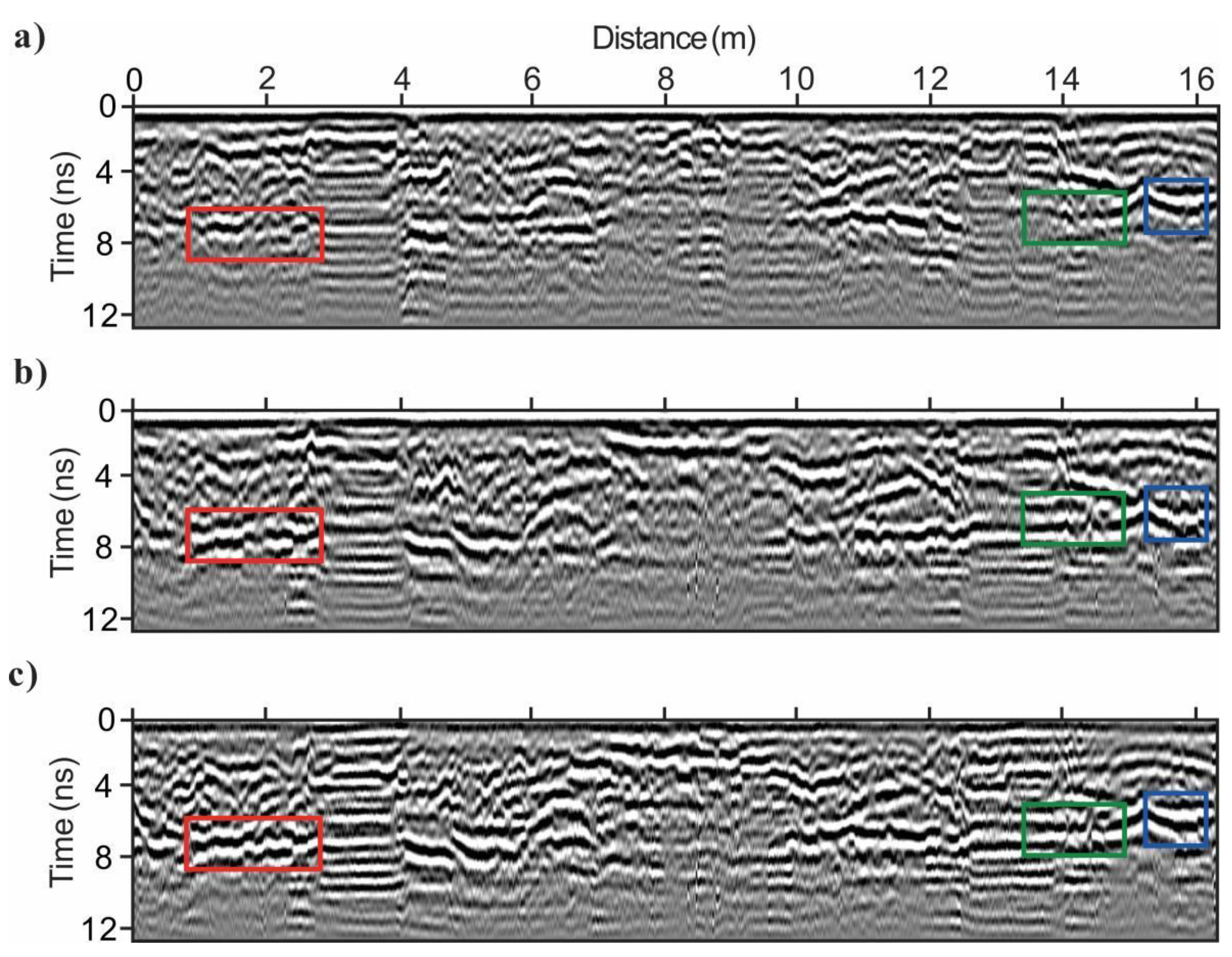
Although the TLFC 3D GPR data were acquired and processed with great consideration, there were still some problems caused by acquisition and processing. If we simply performed difference processing on the time-lapse data, the wavelet characterization of the data could be preserved in the difference profile. Thus, it would be difficult to clearly show the underground changing area (
Figure 7). The time-lapse attribute analysis method proposed by Allroggen et al. has achieved satisfactory results in the time-lapse 2D GPR data of subsurface flow process monitoring [
20,
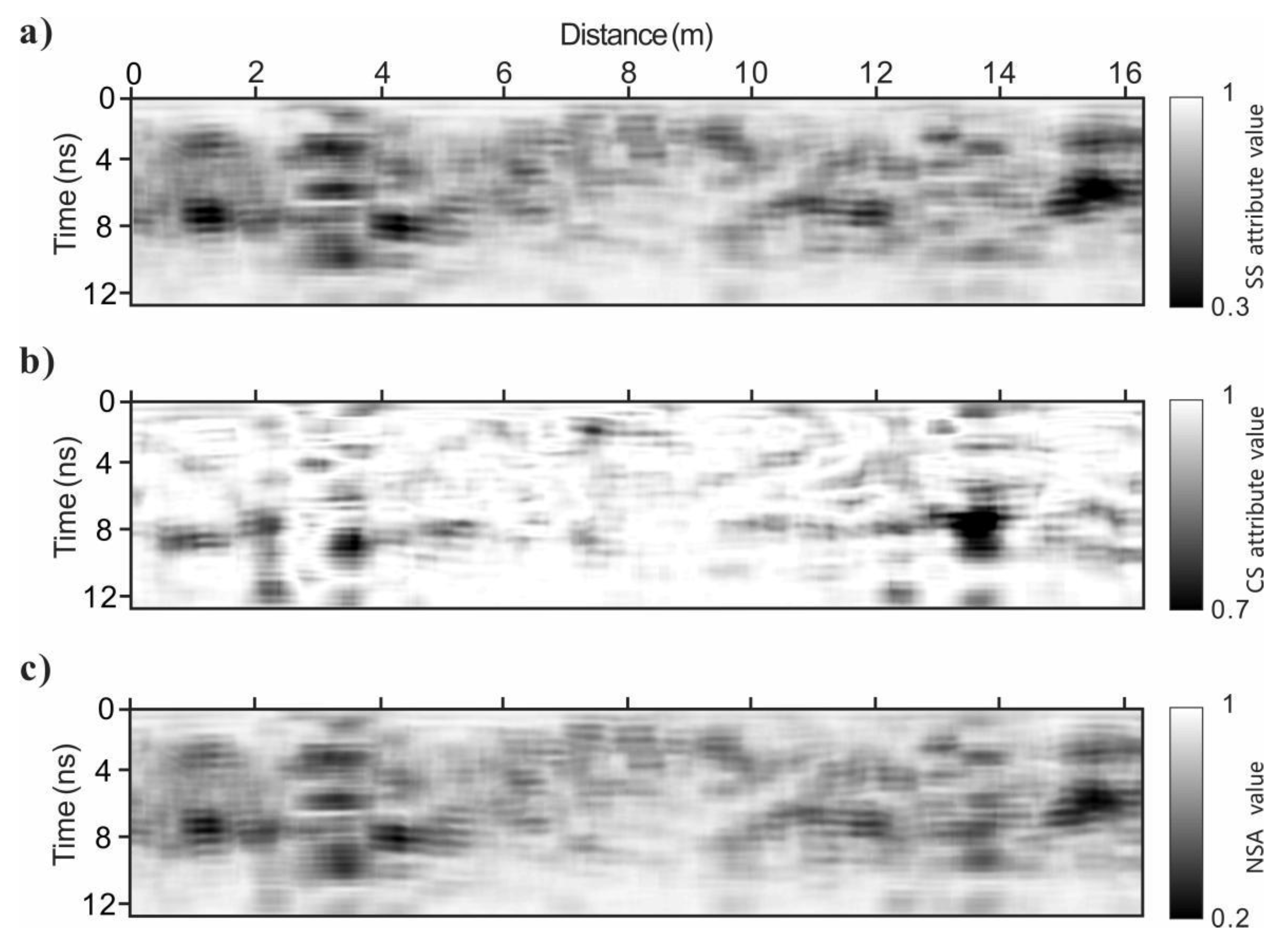
23]. Therefore, we used it for the interpretation of the TLFC 3D GPR road subgrade monitoring data. It includes a contrast similarity (CS) attribute and a structural similarity (SS) attribute. The former mainly reflects the areas where the reflected wave energy is different, and the latter mainly highlights the areas where the shape of the events changes. The CS and SS attributes are respectively defined as follows:
where
and
denote the standard deviations within the selected window,
denotes a normalized zero-lag cross-correlation after subtracting the window means, and
denotes a stable term for avoiding numerical instability when
approaches 0. The specific expression is as follows:
where
and
are the windowed sequences. The normalized similarity attribute (NSA) of the time-lapse data could be obtained by multiplying the CS and SS attributes [
23].
Before calculating the attributes, it is necessary to normalize the amplitude in the selected window, and the value of
is usually 10% of the amplitude variation range in the window after amplitude normalization. During attribute calculation, the window size is the key parameter. With a too-small window, many wavelet features can be retained. Otherwise, it will excessively smooth out the areas with small attribute values. Through parameter experiments, we concluded that the optimal window size for the time-lapse data in this experimental area is 30 × 30. That is, a window contains 30 traces horizontally and 30 sampling points vertically.
Figure 8 shows the attribute calculation results of the time-lapse data on 22 Jul. and 30 Jul. in
Figure 7. A small attribute value denotes low similarity of the time-lapse data, that is, underground changes may have occurred. The SS attribute highlights the areas with different event shapes, and the regions shown in the red and blue boxes in
Figure 7 are highlighted in
Figure 8a. The CS attribute highlights the areas with different reflected wave energies, and the regions shown in the red and green boxes in
Figure 7 are highlighted in
Figure 8b. NSA realizes the fusion of the regions with low attribute values in
Figure 8a,b, and it has a comprehensive display of the underground changing areas.
4.2. Interpretation Based on Attribute Differences
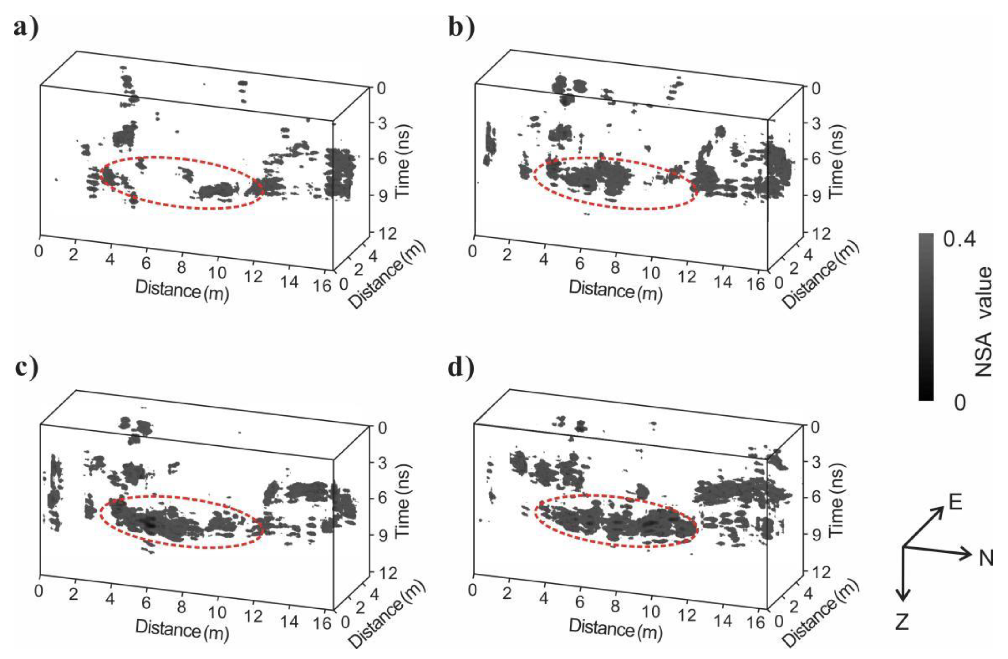
The NSA of the TLFC 3D GPR data was calculated, and 3D images of the results are shown in
Figure 9. Since there were still a few differences caused by nonunderground changes after data processing, when the values of the CS and SS attributes were both less than 0.6 or when any one of them was less than 0.4, we regarded the changes in the data as from underground. Hence, only the parts with NSA values lower than 0.4 were demonstrated, as shown in
Figure 9. The red dotted circle in
Figure 9 corresponds to the near area of the backfill pit 2. Since this area faces the gate of the construction site, it belongs to the key rolling area of the engineering vehicles. The changes in this area are explained as follows.
As time went by, the area with a low NSA value gradually expanded, indicating that the passing of engineering vehicles on this area was continuous during the monitoring period. In addition, according to the changing trend of the attribute value, this area was almost invariable from 22 July to 30 July, and the subgrade was relatively stable. From 30 July to 8 August, the subgrade was dramatically changed, and changes occurred in the southern part. The changing speed of the subgrade tended to ease from 8 August to 22 August, and mainly the northern region has changed. From 22 August to 30 August, the subgrade greatly changed again, mainly in the northern part. It is speculated that the reason for the above changes in the subgrade is that the flow of engineering vehicles was rare before 30 July. Thus, the subgrade could maintain its original structure to a certain extent. From30 Jul. to 8 August, the original structure of the subgrade was damaged and greatly changed due to the frequent passing of engineering vehicles. From 8 Aug. to 22 Aug., the damaged subgrade was compacted to form a new structure. It was difficult for the engineering vehicles to make great changes in the subgrade structure again. Therefore, although the time interval between
Figure 9b,c is two weeks, the change in the low attribute value area was small. From 22 August to 30 August, relatively large changes took place in the low attribute value area, which may be because the subgrade was damaged again due to the passing of a large number of engineering vehicles.
5. Discussion
To overcome the disadvantages of 2D GPR (missing detection and inability to obtain underground dynamic changing information), we proposed a new road subgrade monitoring technology (TLFC 3D GPR), which transformed the traditional detection strategy into a monitoring strategy. The main achievements of this paper are as follows. (1) We presented a method of time zero consistency correction, thus eliminating jitter interference on both sides of events and improving imaging quality. (2) 3D data combination was used in multiple group lines to realize the full-coverage imaging of underground spaces. (3) Thorough spatial position matching well solved the mismatch problem in the time-lapse data. (4) The time-lapse attribute analysis method was applied to interpret the road subgrade monitoring data of TLFC 3D GPR, the wavelet characterization influence was eliminated, and subgrade dynamic changing information was obtained.
Compared with the existing research, this paper mainly has three innovations. First, most road disease studies are based on one-time detection [
5,
17]. Thus, we presented a full-coverage monitoring method and proved its feasibility. Second, the previously proposed time-lapse processing methods are usually based on 2D GPR data [
28,
30,
31,
32]. We realized the data processing of TLFC 3D GPR and improved the imaging quality. Third, the time-lapse attribute has achieved satisfactory results in monitoring the data of 2D GPR for fast subsurface processes [
20,
23]. Thus, we applied it to long-term road subgrade monitoring data with TLFC 3D GPR, and equally excellent results were obtained.
It is worth mentioning that there were still a few differences caused by the nonunderground changes in the processed data, and they may be because of the following reasons. (1) The sampling rate of the instrument fluctuates during data acquisition, resulting in inconsistent time intervals of adjacent sampling points in each trace. (2) The trigger of the ranging wheel may be affected by multiple factors, such as inaccurate encoder positioning, slight topographic relief, and tire pressure changes, resulting in uneven trace spacing. Because the specific impact of the above problems cannot be determined at present, there is no targeted processing, which has caused some interferences to the time-lapse attribute analysis. We could note that some low attribute value areas in
Figure 9 only appeared at an earlier time. Then, the range became smaller or even disappeared.
Moreover, by using TLFC 3D GPR for road monitoring, a massive amount of data can be obtained. At present, manual data processing and interpretation need a lot of time. Therefore, when developing data processing and interpretation methods for TLFC 3D GPR in the future, we should not only pay attention to method accuracy but also to calculation efficiency and automation.
To sum up, in the upcoming research, we will focus on eliminating the influence of the irrelevant variables to ensure that the difference between time-lapse GPR data comes from underground changes to realize the quick and high-precision processing of TLFC 3D GPR data and the accurate characterization of underground 3D spatial changes.
6. Conclusions
In this study, we first put forward a road subgrade monitoring technology based on TLFC 3D GPR. It is an optimal choice for road disease monitoring because of its advantages, which include high data acquisition efficiency, wide-coverage, and the ability to obtain dynamic changing information of underground 3D spaces.
Through time-zero consistency correction, 3D data combination, and spatial position matching of TLFC 3D GPR data, full-coverage and accurate imaging of underground 3D space could be achieved. Furthermore, a time-lapse attribute analysis was performed for the TLFC 3D GPR data. Then, the change rule of the subgrade was comprehensively mastered, and the rapid change period was determined and interpreted.
This paper proves the feasibility of applying TLFC 3D GPR to large-scale road subgrade monitoring, provides a reference for relevant data acquisition, processing, and interpretation, and points out necessary directions for further research.
Author Contributions
Conceptualization, J.L., R.Q., and K.S.; methodology, J.L. and K.S.; validation, J.L., R.Q., K.S., L.G., Y.Z., and D.L.; formal analysis, J.L., R.Q., K.S., L.G., Y.Z., and D.L.; investigation, J.L., K.S., and L.G.; data curation, J.L., R.Q., K.S., and L.G.; writing—original draft preparation, J.L. and Y.Z.; writing—review and editing, R.Q. and K.S.; visualization, J.L., R.Q., and K.S.; supervision, J.L., R.Q., and K.S.; project administration, R.Q.; funding acquisition, R.Q. All authors have read and agreed to the published version of the manuscript.
Funding
This research was funded by the National Natural Science Foundation of China (41974159), Natural Science Foundation of Beijing Municipality (8212016), and 2021 Graduate Innovation Fund Project of China University of Geosciences, Beijing (640221003).
Institutional Review Board Statement
Not applicable.
Informed Consent Statement
Not applicable.
Data Availability Statement
Data associated with this research are available and can be obtained by contacting the corresponding author.
Acknowledgments
The authors especially thank Yuchen Wang and Xu Liu for their field assistance.
Conflicts of Interest
The authors declare no conflict of interest.
References
- Al-Qadi, I.L.; Lahouar, S. Measuring layer thicknesses with GPR-Theory to practice. Constr. Build. Mater. 2005, 19, 763–772. [Google Scholar] [CrossRef]
- Bastard, C.L.; Baltazart, V.; Wang, Y.; Saillard, J. Thin-pavement thickness estimation using GPR with high-resolution and superresolution methods. IEEE Trans. Geosci. Remote Sens. 2007, 45, 2511–2519. [Google Scholar] [CrossRef]
- Liu, H.; Sato, M. In situ measurement of pavement thickness and dielectric permittivity by GPR using an antenna array. NDT E Int. 2014, 64, 65–71. [Google Scholar] [CrossRef]
- Solla, M.; Lagüela, S.; González-Jorge, H.; Arias, P. Approach to identify cracking in asphalt pavement using GPR and infrared thermographic methods: Preliminary findings. NDT E Int. 2014, 62, 55–65. [Google Scholar] [CrossRef]
- Kim, N.; Kim, S.; An, Y.; Lee, J. A novel 3D GPR image arrangement for deep learning-based underground object classification. Int. J. Pavement Eng. 2019, 22, 740–751. [Google Scholar] [CrossRef]
- Torbaghan, M.E.; Li, W.; Metje, N.; Burrow, M.; Chapman, D.N.; Rogers, C.D.F. Automated detection of cracks in roads using ground penetrating radar. J. Appl. Geophys. 2020, 179, 104118. [Google Scholar] [CrossRef]
- Poikajärvi, J.; Peisa, K.; Herronen, T.; Aursand, P.O.; Maijala, P.; Narbro, A. GPR in road investigations-equipment tests and quality assurance of new asphalt pavement. Nondestr. Test. Eval. 2012, 27, 293–303. [Google Scholar] [CrossRef]
- Rodés, J.P.; Reguero, A.M.; Pérez-Gracia, V. GPR spectra for monitoring asphalt pavements. Remote Sens. 2020, 12, 1749. [Google Scholar] [CrossRef]
- Bezina, Š.; Stančerić, I.; Domitrović, J.; Rukavina, T. Spatial representation of GPR data-accuracy of asphalt layers thickness mapping. Remote Sens. 2021, 13, 864. [Google Scholar] [CrossRef]
- Grote, K.; Hubbard, S.; Rubin, Y. GPR monitoring of volumetric water content in soils applied to highway construction and maintenance. Lead. Edge 2002, 21, 482–485. [Google Scholar] [CrossRef] [Green Version]
- Benedetto, A.; Tosti, F.; Ortuani, B.; Giudici, M.; Mele, M. Mapping the spatial variation of soil moisture at the large scale using GPR for pavement applications. Near Surf. Geophys. 2015, 13, 269–278. [Google Scholar] [CrossRef]
- Rodés, J.P.; Pérez-Gracia, V.; Martínez-Reguero, A. Evaluation of the GPR frequency spectra in asphalt pavement assessment. Constr. Build. Mater. 2015, 96, 181–188. [Google Scholar] [CrossRef] [Green Version]
- Solla, M.; Pérez-Gracia, V.; Fontul, S. A review of GPR application on transport infrastructures: Troubleshooting and best practices. Remote Sens. 2021, 13, 672. [Google Scholar] [CrossRef]
- Grasmueck, M.; Weger, R.; Horstmeyer, H. Full-resolution 3D GPR imaging. Geophysics 2005, 70, K12–K19. [Google Scholar] [CrossRef]
- Gaballah, M.; Grasmueck, M.; Sato, M. Characterizing subsurface archaeological structures with full resolution 3D GPR at the early dynastic foundations of saqqara necropolis, Egypt. Sens. Imaging 2018, 19, 23. [Google Scholar] [CrossRef]
- Dinh, K.; Gucunski, N.; Tran, K.; Novo, A.; Nguyen, T. Full-resolution 3D imaging for concrete structures with dual-polarization GPR. Autom. Constr. 2021, 125, 103652. [Google Scholar] [CrossRef]
- Liu, Z.; Wu, W.; Gu, X.; Li, S.; Wang, L.; Zhang, T. Application of combining YOLO models and 3D GPR images in road detection and maintenance. Remote Sens. 2021, 13, 1081. [Google Scholar] [CrossRef]
- Mangel, A.R.; Lytle, B.A.; Moysey, S.M.J. Automated high-resolution GPR data collection for monitoring dynamic hydrologic processes in two and three dimensions. Lead. Edge 2015, 34, 190–196. [Google Scholar] [CrossRef]
- Allroggen, N.; van Schaik, N.L.M.B.; Tronicke, J. 4D ground-penetrating radar during a plot scale dye tracer experiment. J. Appl. Geophys. 2015, 118, 139–144. [Google Scholar] [CrossRef]
- Allroggen, N.; Tronicke, J. Attribute-based analysis of time-lapse ground-penetrating radar data. Geophysics 2016, 81, H1–H8. [Google Scholar] [CrossRef]
- Pan, X.; Jaumann, S.; Zhang, J.; Roth, K. Efficient estimation of effective hydraulic properties of stratal undulating surface layer using time-lapse multi-channel GPR. Hydrol. Earth Syst. Sci. 2019, 23, 3653–3663. [Google Scholar] [CrossRef] [Green Version]
- Saito, H.; Kuroda, S.; Iwasaki, T.; Sala, J.; Fujimaki, H. Estimating infiltration front depth using time-lapse multioffset gathers obtained from ground-penetrating-radar antenna array. Geophysics 2021, 86, WB109–WB117. [Google Scholar] [CrossRef]
- Allroggen, N.; Beiter, D.; Tronicke, J. Ground-penetrating radar monitoring of fast subsurface processes. Geophysics 2020, 85, A19–A23. [Google Scholar] [CrossRef]
- Johnson, T.C.; Routh, P.S.; Barrash, W.; Knoll, M.D. A field comparison of fresnel zone and ray-based GPR attenuation-difference tomography for time-lapse imaging of electrically anomalous tracer or contaminant plumes. Geophysics 2007, 72, G21–G29. [Google Scholar] [CrossRef] [Green Version]
- Steelman, C.M.; Klazinga, D.R.; Cahill, A.G.; Endres, A.L.; Parker, B.L. Monitoring the evolution and migration of a methane gas plume in an unconfined sandy aquifer using time-lapse GPR and ERT. J. Contam. Hydrol. 2017, 205, 12–24. [Google Scholar] [CrossRef] [PubMed]
- Yuan, H.; Looms, M.C.; Nielsen, L. On the usage of diffractions in GPR reflection data-implications for time-lapse gas migration monitoring. Geophysics 2020, 85, H83–H95. [Google Scholar] [CrossRef]
- Dérobert, X.; Baltazart, V.; Simonin, J.; Todkar, S.S.; Norgeot, C.; Hui, H. GPR monitoring of artificial debonded pavement structures throughout its life cycle during accelerated pavement testing. Remote Sens. 2021, 13, 1474. [Google Scholar] [CrossRef]
- Luo, T.X.H.; Lai, W.L.W. Subsurface diagnosis with time-lapse GPR slices and change detection algorithms. IEEE J. Sel. Top. Appl. Earth Observ. Remote Sens. 2020, 13, 935–940. [Google Scholar] [CrossRef]
- Ciampoli, L.B.; Gagliardi, V.; Clementini, C.; Latini, D.; Frate, F.D.; Benedetto, A. Transport infrastructure monitoring by InSAR and GPR data fusion. Surv. Geophys. 2020, 41, 371–394. [Google Scholar] [CrossRef]
- Friedt, J. Passive cooperative targets for subsurface physical and chemical measurements: A systems perspective. IEEE Geosci. Remote Sens. Lett. 2017, 14, 821–825. [Google Scholar] [CrossRef]
- Allroggen, N.; Jackisch, C.; Tronicke, J. Four-Dimensional Gridding of Time-Lapse GPR Data. In Proceedings of the 9th International Workshop on Advanced Ground Penetrating Radar (IWAGPR), Edinburgh, UK, 28–30 June 2017. [Google Scholar]
- Giertzuch, P.; Doetsch, J.; Jalali, M.; Alexis, S.; Schmelzbach, C.; Maurer, H. Time-lapse GPR difference reflection imaging of saline tracer flow in fractured rock. Geophysics 2020, 85, H25–H37. [Google Scholar] [CrossRef]
- Haarder, E.B.; Looms, M.C.; Jensen, K.H.; Nielsen, L. Visualizing unsaturated flow phenomena using high-resolution reflection ground penetrating radar. Vadose Zone J. 2011, 10, 84–97. [Google Scholar] [CrossRef]
- Cheung, W.Y.B.; Lai, W.L.W. Field validation of water-pipe leakage detection through spatial and time-lapse analysis of GPR wave velocity. Near Surf. Geophys. 2019, 17, 231–246. [Google Scholar] [CrossRef]
| Publisher’s Note: MDPI stays neutral with regard to jurisdictional claims in published maps and institutional affiliations. |
© 2022 by the authors. Licensee MDPI, Basel, Switzerland. This article is an open access article distributed under the terms and conditions of the Creative Commons Attribution (CC BY) license (https://creativecommons.org/licenses/by/4.0/).


