Article

Deriving Nutrient Concentrations from Sentinel-3 OLCI Data in North-Eastern Baltic Sea

1
Department of Remote Sensing and Marine Optics, Estonian Marine Institute, University of Tartu, Mäealuse 14, 12618 Tallinn, Estonia
2
Chair of Hydrobiology and Fishery, Institute of Agricultural and Environmental Sciences, Estonian University of Life Sciences, Kreutzwaldi 5, 51006 Tartu, Estonia
3
Department of Marine Biology, Estonian Marine Institute, University of Tartu, Mäealuse 14, 12618 Tallinn, Estonia
*
Author to whom correspondence should be addressed.
Remote Sens. 2022, 14(6), 1487; https://doi.org/10.3390/rs14061487
Submission received: 4 February 2022 / Revised: 14 March 2022 / Accepted: 17 March 2022 / Published: 19 March 2022

Abstract

:
Nutrients are important elements in marine ecosystems and water quality, and have a major role in the eutrophication of water bodies. Monitoring nutrient loads is especially important for the Baltic Sea, which is especially sensitive to the eutrophication. Using optical remote sensing data in mapping total nitrogen (TN) and total phosphorus (TP) is challenging because these substances do not have a direct influence on the water optics that remote sensing sensors can detect. On the other hand, it would be very rewarding. In this study, more than 25,000 Sentinel-3 Ocean and Land Colour Instrument (OLCI) data algorithms were tested in order to detect the TN and TP concentrations in the Estonian marine waters between 2016–2021. The TN estimations were well derived for Estonian marine waters (R2 = 0.73, RMSE = 4.87 µmolN L−1, MAPE = 14%, n = 708), while the TP estimations were weaker (R2 = 0.38, RMSE = 0.23 µmolP L−1, MAPE = 24%, n = 730). The Estonian marine waters were divided into six geographic regions in order to study the effect of regional water quality on the TN and TP retrievals. The nutrient concentrations were derived in every region when spring and summer periods were treated separately. In this study, the detection of both nutrients was more successful in more closed areas with P deficiency, while in open sea areas it was more challenging. This study shows that it is possible to estimate nutrients, especially TN, from remote sensing data. Consequently, remote sensing could provide a reliable support to the conventional monitoring by covering large marine areas with high temporal and spatial resolution data.

Graphical Abstract

1. Introduction

Baltic Sea is the world’s largest inland brackish water sea and is very well studied. Eutrophication has been evident in the Baltic Sea for many decades, due to past high and still excessive loads of total nitrogen (TN) and total phosphorus (TP) [1]. The combination of a large catchment area with a high rate of human activities and a small body of water with limited exchange with the Atlantic Ocean through the narrow and shallow Skagerrak makes the Baltic Sea very sensitive to nutrient enrichment and eutrophication. Therefore, in the Baltic Sea, the large input of nutrients like phosphorus and nitrogen is a major environmental concern [2]. The conventional in situ water quality monitoring has failed to characterize nutrient dynamics because of the limitations in spatial sampling and poor availability of reliable data for nutrient loads [3,4].
Nutrient concentrations are very important because they cause eutrophication—an increase in aquatic biomass. Phytoplankton biomass is usually characterised by chlorophyll-a (Chl-a) concentration. Therefore, the Chl-a is the primary indicator of the waterbody ecological state [4,5]. In the Baltic Sea, the open basins are mainly nitrogen limited, especially in spring, when the spring phytoplankton bloom is peaking. In summer, massive blooms of nitrogen fixing cyanobacteria occur in the Baltic Sea. They are driven by excess phosphorus, along with high temperatures. The cyanobacterial blooms contribute significant quantities of new nitrogen to the pelagic ecosystem, hence reducing phosphorus loads is very important to reduce those blooms [4]. To develop an effective nutrient management strategy, better understanding of the Baltic Sea ecosystem is required [1].
Although nutrient concentrations are important water quality indicators in coastal waters, and at the same time the Baltic Sea is often claimed as the most studied sea in the world, the quality of regional monitoring of the nutrient pollution entering the area remains relatively poor [4,6]. Remote sensing has the abilities that could be highly beneficial to marine monitoring—it provides high spatial and temporal resolution which is impossible to achieve with in situ measurements. This is beneficial even if remote sensing cannot provide similar accuracy as the time consuming and expensive laboratory methods. Consequently, combining both conventional in situ sampling and remote sensing methods should be the most optimal way to study the marine environment, provided the remote sensing methods can provide sufficient accuracy.
The European Union’s Earth observation programme, the Copernicus program [7], has launched a mission Sentinel-3, which is a constellation of two satellites (A and B, launched in 2016 and 2018, respectively) [8]. Sentinel-3 has a medium resolution (300 m) Ocean and Land Colour Instrument (OLCI) onboard for marine and land research. It has 21 spectral bands and provides global coverage (at the equator) every two days. OLCI was built for marine monitoring and has well placed spectral bands for that purpose (ESA Sentinel Online).
Remote sensing has been widely used for water quality monitoring [9,10,11,12,13,14,15,16,17,18,19,20,21,22,23,24], because of its large advantage in temporal and spatial coverage compared with in situ methods. So far, most studies have focused on water quality variables, such as Chl-a, turbidity or transparency (measured with Secchi disk depth, SD), total suspended solids (TSS), and coloured dissolved organic matter (CDOM), which all are optically active substances. Remote sensing presents a challenge in estimating nutrients like TN and TP concentration in water, because they have no direct optical properties and spectral characteristics [25]. However, nutrients like TN and TP can be highly correlated with optically active variables that can be estimated by remote sensing [22,26]. When nutrients concentrations are in good correlation with some optical properties of water, the optical parameter can be used as a proxy for TN and/or TP. The previous work testing the retrieval of the optical parameters in the Baltic Sea based on OLCI data with Case 2 Regional CoastColour (C2RCC) atmospheric correction have given good results [27]. However, some studies have found only the band ratios based on the reflectances to work well, and not the Level-2 products themselves [11,17].
Remote sensing techniques have been used to estimate different forms (total, inorganic, etc.) of nitrogen and phosphorus in freshwater bodies [18,26,28,29,30,31,32,33,34,35,36,37,38]. Although less studies have been carried out in sea water [3,5,39,40], the results have been encouraging with errors as low as 11% for TN and 13% for TP [3]. While most studies in marine waters are focusing on detecting TN or/and other forms of nitrogen, there are only a few attempting to detect TP [40]. The chosen methods are either the neural network [3] and machine learning approaches [5,40], or multiple stepwise [39] regression models.
The main objective of current work was to find the best algorithms for estimating the concentrations of TN and TP in Estonian marine waters using Sentinel-3 OLCI data. In addition, the temporal and spatial variability of the best algorithms were studied to estimate nutrients with the highest possible accuracy. Accurate algorithms would give the possibility to monitor the nutrients over large spatial scales and with high temporally frequency, which is not possible with conventional methods. This is the first time where remote sensing with regionally tuned algorithms for nutrient estimations have been used in the north-eastern Baltic Sea.

2. Materials and Methods

2.1. In Situ Dataset and Study Area

In the current study, the measurements from the Estonian National Monitoring Program were used. In total, 2103 TN and 2078 TP measurements were carried out during 2016–2021 in Estonian marine waters (approx. 36,500 km2 (~10%) area of the Baltic Sea). Water samples for both nutrients were collected from 1 m depth. Unfortunately, the optical parameters, like the Chl-a, SD, TSS and the absorption of CDOM at 400 nm (aCDOM) were not always measured together with the nutrients. The database included 1387 Chl-a, 1162 SD, 49 TSS, and only 39 aCDOM measurements.
To eliminate the possible effect from the coast or the seafloor on the remote sensing signal, 29 sampling stations (382 TN and 378 TP measurements) that were closer than 1 km from the shore were removed from the analysis. After this elimination, the database contained 63 sampling stations with 1721 TN and 1700 TP measurements in total. All the stations used in the study are shown in Figure 1.
In this study, the Estonian marine waters were divided into six geographical regions (R1–R6; Figure 1) based on the § 324(4) of the Estonian Water Act [41], because there are large differences in the characteristics of the regions. Division used in the current study is similar to the state classification of the coastal waters in the Estonian Water Act, with the difference being that we included the territorial waters and the exclusive economic zone (EEZ) of the six regions together with the internal waters. The main characteristics of the six regions are:
  • R1: south-east area of the Gulf of Finland. It is oligohaline (2.5–6 ppt) open water with measured max Chl-a 29.5 mg m−3 and min SD 0.8 m during 2016–2021. The largest inlet in region R1 is the Narva River. Twelve sampling stations were in this region.
  • R2: Pärnu Bay is located in the north-eastern part of the Gulf of Riga. The bay is semi-enclosed, oligohaline (4.0–5.5 ppt), with a large inlet of nutrient rich Pärnu river. During 2016–2021, the measured max Chl-a was 45 mg m−3 and min SD 0.4 m. It is the smallest region by area (411 km2), and the max depth in the mouth of the bay is 12 m. Four sampling stations were included in this region.
  • R3: western part of Gulf of Finland, it has mesohaline (4.5–6.5 ppt) and deep water with measured max Chl-a 25.3 mg m−3 and min SD 2 m during 2016–2021. Sixteen sampling stations were in this region.
  • R4: Baltic Proper area of the West Estonian archipelago, open sea, with mesohaline (6–7 ppt) water. Region R4 is a shallow area open to waves with measured max Chl-a 15.6 mg m−3 and min SD 3 m during 2016–2021. Seventeen sampling stations were in this region.
  • R5: Väinameri Sea or the Sea of Straits (2200 km2); it has mesohaline (3–6.5 ppt) unstratified water, and it is a shallow, concealed area with measured max Chl-a 6.7 mg m−3 and min SD 1.2 m during 2016–2021. Seven sampling stations were in this region.
  • R6: north half of Gulf of Riga with mesohaline (4–6 ppt), shallow, sheltered and seasonally stratified waters with measured max Chl-a 71.8 mg m−3 and min SD 0.5 m during 2016–2021. Seven sampling stations were in this region.

2.2. In Situ Parameters

The TN and TP concentrations were measured by the accredited Estonian Marine Institute’s laboratory with a continuous flow automated wet chemistry analyser Skalar SANplus (Skalar Analytic B.V.,DeBreda, The Netherlands), using the standard methods EN ISO 11905-1 and EN ISO 15681-2. Detection limits were 10 µg L−1 for both TN and TP, and measurement uncertainty did not exceed 25%.
Temperature and salinity data were extracted from the CTD profiles, measured with the Sea and Sun Technology M90 or SAIV SD201 probes. The Chl-a concentration in a sample was determined spectrophotometrically (light absorption) using ISO 10260 standard and HELCOM guidelines [42]. Water transparency (SD) was measured with a standard Secchi disk.
Absorption by CDOM, aCDOM, was measured spectrophotometrically with a PERKIN ELMER Lambda 35 UV/VIS spectrometer in the range 350–750 nm from a filtered (Millex 0.22 μm) water sample in a 10 cm cuvette against distilled water. The measurements were corrected for residual scattering according to Davies-Colley and Vant [43], and a final calculation for aCDOM at 400 nm was conducted by Lindell et al. [44].

2.3. Sentinel-3 Dataset

The processing of the Copernicus Sentinel-3 OLCI Level-1 (300 × 300 m resolution) data was done using the Estonian national satellite data centre portal for Earth observation data processing [45]. This platform has Sentinel-3 OLCI Level-1 archive and atmospheric correction tools. For atmospheric correction, the C2RCC v.1.5 processor [46] with the multisensor pixel identification tool (IdePix) were used. In extracting the match-ups, the same day 1 × 1 pixels with the sampling stations date and location were used. The 1 × 1 pixel size was used because a single OLCI pixel is large, and many in situ locations were close to each other. Pixels with cloud or other quality flags (except the “quality_flags.sun_glint_risk” flag) were removed from further analyses.
In total, 741 same-day cloud-free match ups (including Sentinel-3A and -3B) during 2016–2021 were found for TP and 719 for TN. The most match ups were from May to July (Table 1). There were no cloud-, ice- or snow-free match-ups in January, February, March and December.

2.4. TN and TP Retrieval Methods

Fifteen different formulas were used with the atmospherically corrected angular dependent water-leaving reflectance (C2RCC reflectances) and the C2RCC processor Level-2 (L2) products for the retrieval of TN and TP (Table 2). Only the general formulas used in this study are shown in the Table 2. Every formula was tested with different combinations by altering C2RCC reflectances on the 15 bands, and the 13 different C2RCC L2 products (Table 3) were included only to the simplest formulas (1–4 in Table 2). In total, 25,013 different algorithms were made for testing.
To find the best algorithm for deriving TN and TP, a quadratic polynomial regression model was used similarly by Huang et al. [35] in Xiangxi Bay, China. Equation (1) was used to derive TN or TP concentrations.
y = ax2 + bx + c
where y is the derived TN or TP, x is the algorithm of L2 product or band ratios, and a, b, and c are the polynomial regression coefficients.
The entire match up database was tested with over 25,000 algorithms, but also every region (R1–R6) separately was tested on six different temporal divisions:
  • April to November;
  • May to September;
  • April to May;
  • June to September;
  • April to June;
  • July to September.
The first period includes all data. The second period (May to September) is agreed in the monitoring program as the biologically active period. For example, the indicator for eutrophication in the monitoring program is mean Chl-a for the May–September period. The third and fourth periods are the traditional way to divide spring and summer between months (April to May and June to September, accordingly). Lastly, the fifth and sixth periods are the new way to define spring and summer seasons, to distinguish the spring bloom from the summer cyanobacteria bloom (April to June and July to September, accordingly).
In addition, three combined regions were formed: the Gulf of Finland (R1 + R3), west Estonian archipelago waters and the Baltic Proper (R4 + R5), and the Gulf of Riga (R2 + R6). All of them were used to test all the algorithms on the six temporal divisions.

2.5. Statistical Analysis

Mean values were used to describe in situ characteristics. The mean is the average value of the dataset.
The performance of algorithms was evaluated using the determination coefficient (R2). R2 is used to analyze how well observed in situ values are predicted by the model based on the proportion of total variation of outcomes explained by the model; it is calculated using Equation (2).
R 2 = 1 i = 1 n y i y ^ 2 i = 1 n y i y ¯ 2
where, y ^ is the predicted value, y is the observed value, y ¯ is the mean value of observed y values, and n is the number of observations.
To evaluate the error of the derived nutrients, root mean squared error (RMSE) and bias were used (both are in the same units as the quantity being estimated). RMSE is a frequently used measure of differences between values observed in situ and predicted by a model; it is calculated using Equation (3). Bias shows a systematic error, and it is calculated using Equation (4).
RMSE = 1 n i = 1 n y ^ y i 2
bias = 1 n i = 1 n y ^ y i
where, y ^ is the predicted value, y is the observed value, and n is the number of observations.
In addition, the performance of algorithms was evaluated using accuracy through the mean absolute percentage error (MAPE). MAPE measures the percentage error of the estimated values in relation to the actual values; it is calculated using Equation (5).
MAPE = 100 % n i = 1 n y i y ^ i y i
where, y ^ is the predicted value, y is the observed value, and n is the number of observations. Accuracy represents correctly predicted values (expressed as a percentage). Accuracy is calculated as 100 MAPE .
The 95% confidence interval value (95%CI) is used to describe the uncertainties associated with the quadratic polynomial regression model, and it is presented for the coefficients of the regression model. It is calculated using Equations (6) and (7), where sefit is the unbiased estimate of the standard error of the fit, and tcrit is the critical value of the t distribution with degrees of freedom of the residuals with significance level 0.05/2.
CI = ± s e f i t × t c r i t
s e fit = s s r e s d f r e s × X 0 T ( X T X ) 1 X 0
where, ssres is the sum of squares for the residuals, dfres is the degrees of freedom for the residuals, X0 is the column array and X is the design matrix of the observed values, and T notes the transposed matrix.

3. Results

3.1. Match-Up In Situ Database
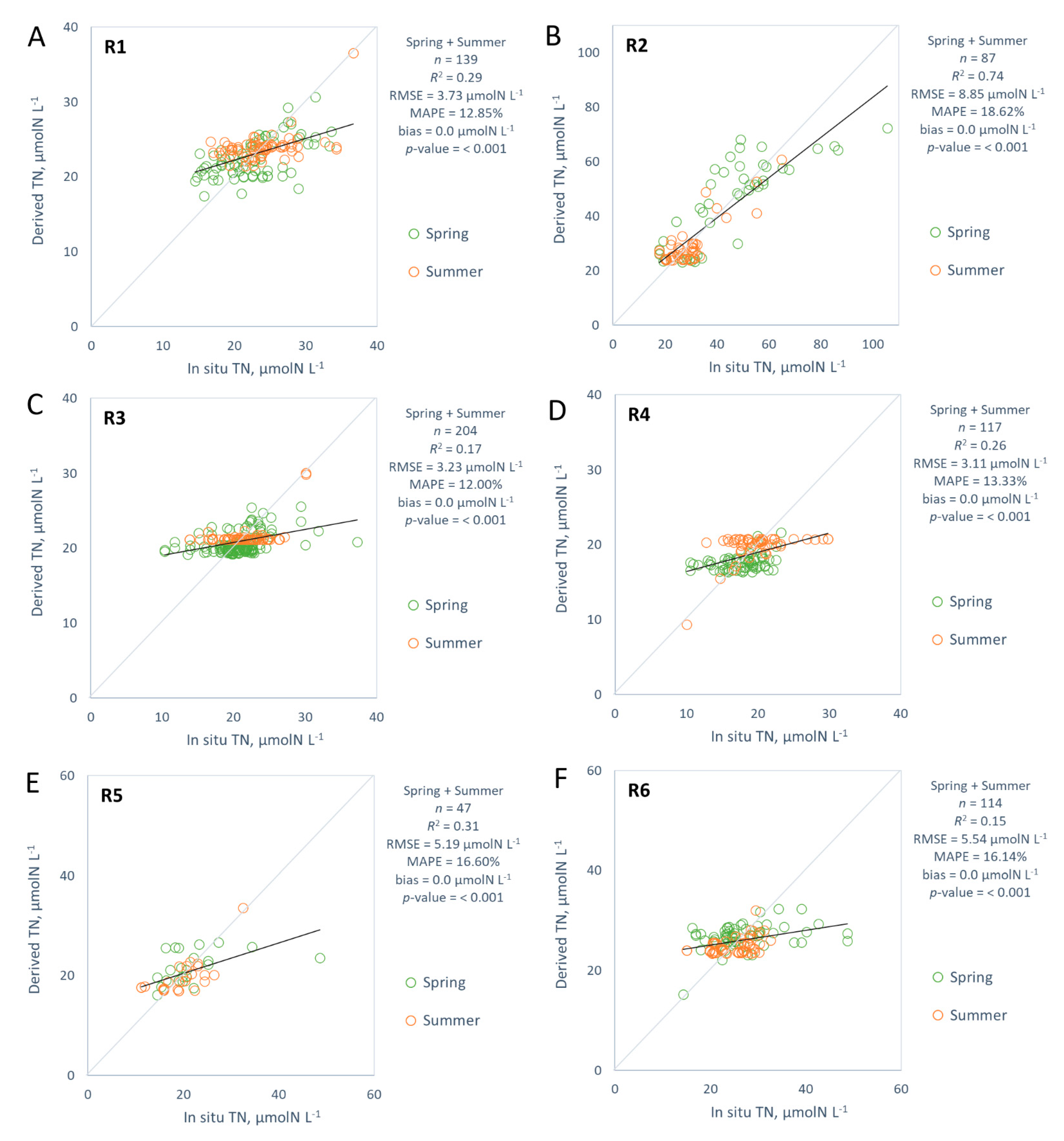
The means of the in situ TN, TP, TN:TP, Chl-a and SD in different regions and seasons of the match-ups stations are shown in Table 4. The means of the nutrients, and especially the TN:TP ratios, are not very different between the seasons, except in some regions like R2 and R5. The SD in region R2 is significantly lower than in other regions. The Chl-a in spring is the highest in regions R2 and R6 (Table 4).
The strongest relationships between in situ Chl-a and in situ TN were in the region R1 summer season, and in the rest of the regions no remarkable relationship was shown. The TP did also not have any relationship with Chl-a, except in the region R4 in spring (Figure 2A). The transparency and TP had the strongest relationship in only region R5 (spring and summer) and in the summer periods of regions R2 and R4 (Table 5). The relationship between in situ TN and SD seems to be exponential rather than linear. For example, in spring period the R2 was 0.27 with linear regression, but 0.39 with exponential regression (Table 5; Figure 2B). All the linear regressions between the in situ TN and TP and the in situ optically active substances within the match-up dataset according to the regions and seasons are shown in Table 5.
The match-up in situ database showed strong dependence of TN with aCDOM (R2 = 0.78, n = 21, p-value = 1E−07), but only a weak relationship between TP and aCDOM (R2 = 0.19, n = 21, p-value = 0.05) (Figure 3). Within the match-up in situ dataset, the relationships with TSS were not significant (TP: R2 = 0.13, n = 18, p-value = 0.15 and TN: R2 = 0.09, n = 18, p-value = 0.22), though with a larger dataset some relationships might occur.

3.2. Total Nitrogen

After testing over 25,000 band/product ratio combinations on the 719 TN match-ups, the highest R2 for each region (R1–R6) and each temporal division is shown in Table 4 with the combinations of regions and with no regions results. The highest R2 was usually in the shortest period: April to May. Although the highest R2 was in April to May, the combination of April to June + July to September periods was chosen in the current study. There are two reasons for that: (1) the algorithms worked much better in all regions in the July to September period than in the June to September period; (2) too low count of match-ups in the April to May period in R5 (n = 9) made the polynomial regression results unreliable (Table 6).
Generally, the option with no regions applied was performing rather well in all temporal divisions (R2 ranged between 0.31–0.64). In comparison of different regions, the algorithms were performing very well in R2. In the R3 and R6 regions, the performance was the weakest along all the temporal divisions (Table 6). The combination of regions did not improve the results and it was not used in the further study. Not using any regions might be a simple option for fast results, but using regions improves the MAPE of the deriving TN for the entire vegetation season (April to September) from 18.2% to 14.2% (Figure 4). The overall results in the different regions not applied and all regions combined versions for the entire vegetation period were relatively good: R2 from 0.52 to 0.73, with RMSE from 6.5 to 4.9 µmolN L−1, respectively (Figure 2).
There were significant differences in deriving TN in different regions. The strongest relationship with TN was in region R2 (Pärnu Bay) (R2 = 0.74), while the weakest relationship was in regions R3 and R6 (R2 = 0.17 and 0.15, respectively) (Figure 5). The RMSE was between 3.11 to 8.85 µmolN L−1 (regions R4 to R2, respectively). Although the region R2 had the strongest relationship towards TN, the accuracy was the lowest (81.4%), because the absolute values of TN were at least twice as high compared with other regions. In region R2, the TN max is 105.6 µmolN L−1, while in other regions, the TN max ranges from 29.8 µmolN L−1 to 48.6 µmolN L−1.
The statistics of the spring and summer seasons separately are shown in Table 7 with the formulas used. All the results are significant, except in R5 spring, where the p-value is 0.05. In addition, the coefficients of the quadratic polynomial regression model (a, b and c with the 95% confidence interval values (95%CI)) used in deriving TN are shown in Table 8. Only regions R2 and R4 in the summer periods have the same band ratio formula with the exact same bands. Almost half of the used formulas have the L2 product in them. In regions R3 and R6, the total particle scattering and either TSS or Chl-a concentrations gave the best results in summer period. In region R4, the best way to evaluate TN in spring is through the phytoplankton pigments and CDOM. The transparency products (Kd) are used in regions R3 and R5. Regions R1 and R2 algorithms used only reflectances in both periods. Only the reflectance bands at 400 and 442.5 nm were not used (Table 7). From the Table 6 and Table 7 (and Figure 4), it is evident that deriving TN is challenging in most of the regions (R1, R3, R4 and R6), and more in the spring period than in summer (MAPE is always higher in spring).

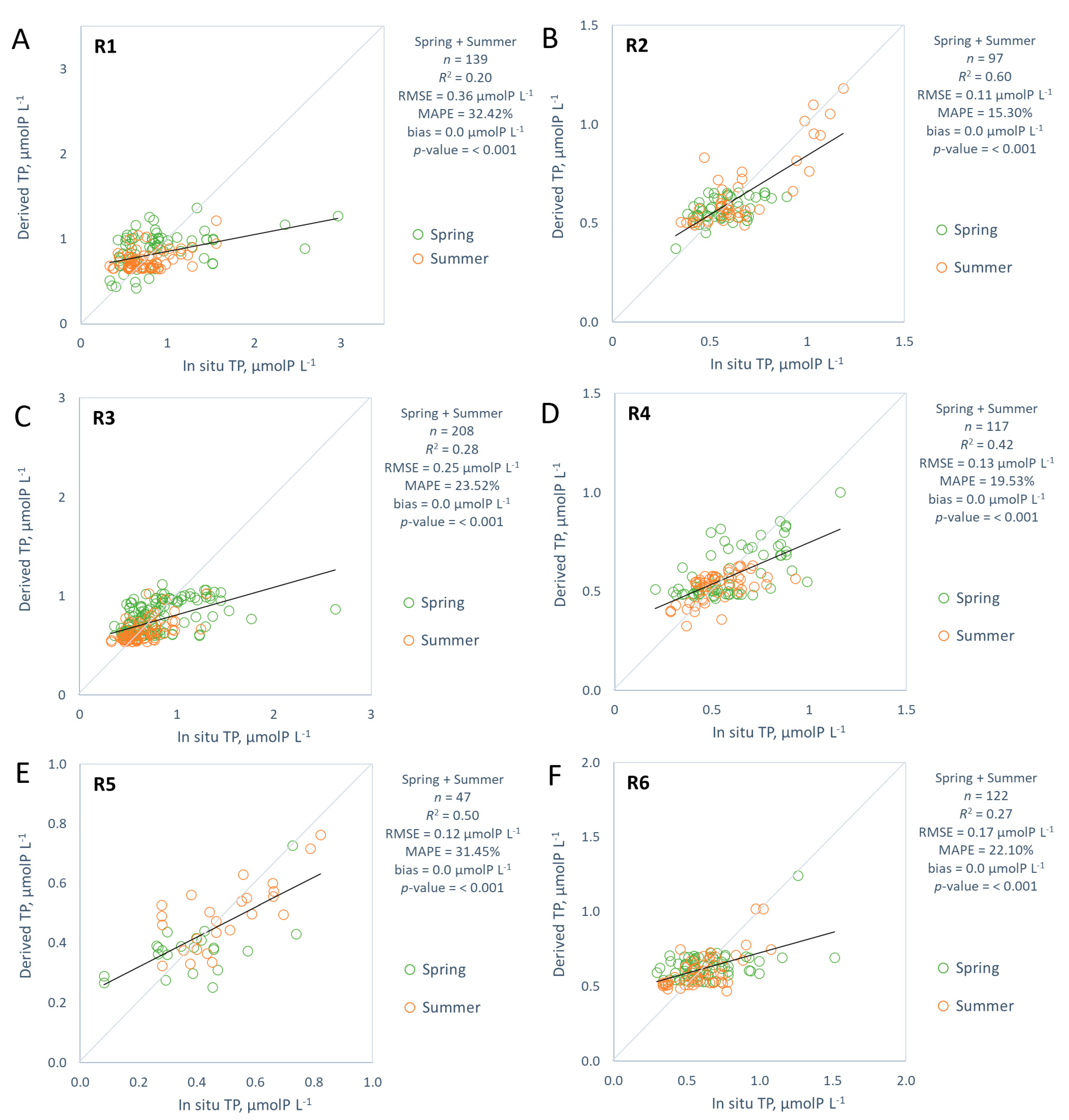
3.3. Total Phosphorus

There were more TP measurements than TN; the TP database contained 741 TP match-ups. The highest R2 for each region (R1–R6) and each temporal division is shown in Table 9. Additionally, similar to TN, combinations of different regions and no regions were used for algorithm testing. Generally, the relationships between derived algorithms and TP were weaker than with TN. The highest R2 was usually found for the shortest period, April to May; however, at the same time, the July to September period gave very good results compared to other time divisions. For the same reasons as for TN, April to June + July to September periods were chosen for this study.
On the contrary to TN, the algorithms were performing very poorly in all temporal divisions when no regions were differenced (R2 ranged 0.06–0.16). Using regions improves the accuracy of the estimation of TP for all the temporal divisions (Table 8). Similarly with TN estimations, algorithms performed better in regions R2 and R5; in the R1, R3 and R6 regions, the performance was the weakest along all the temporal divisions. The combination of geographically-close regions (R1 + R3, R2 + R6, and R4 + R5) did not improve the estimation of TP, and therefore was excluded from the further study (Table 9). The accuracy of the TP estimation improves from 69.9% to 76.2% (R2 from 0.15 to 0.38) for the entire vegetation period (April to September) when regions are applied to the dataset (Figure 6).
The accuracy of estimating TP concentrations had significant differences between the different regions, being highest in region R2, at 84.7%, and lowest in region R1, at 67.6% (Figure 7). In all the cases, the remote sensing algorithms were underestimating TP concentrations. Still, the detection of TP was better in regions R2, R4, and R5 (R2 was 0.60, 0.42 and 0.50, accordingly). The RMSE was between 0.11 and 0.36 µmolP L−1.
Table 10 and Table 11 show the best formulas and the coefficients used in TP deriving algorithms. Similarly with TN algorithms, almost half of the formulas have L2 products in them. In region R5, Chl-a and scattering of the marine particles seems to be influencing TP in spring, compared to CDOM together with TSS and pigments in summer. The best algorithms for regions R1 and R6 have relationships with transparency L2 products (Kd). The algorithms for regions R2 and R3 used only reflectance bands. The reflectance bands on 560–620 nm and 709–754 nm were not used in any of the best algorithms. In deriving TP, the spring season had lower R2 and higher MAPE (with some exceptions (R2 and R4)) compared with the summer season (Table 10).

4. Discussion

The detection of nutrients from optical remote sensing data still remains a challenge because TN and TP have no spectral response in the visible and near-infrared regions [25]. Several studies have estimated the nitrogen and phosphorus based on their strong relationships with Chl-a, TSS, and other optically sensitive parameters in the water [5,26,34,35,47,48,49]. In addition, a previous study has shown that Chl-a and SD are able to explain 41% of the variance in TP for the Swedish rivers discharging into the Baltic Sea [30]. Unfortunately, in the current study, no strong relationships were observed between the in situ Chl-a or SD with the nutrients in the match-up dataset (Table 5). TN showed only a moderate relationship with Chl-a in the R1 region. TP only had a significant relationship in the R4 region during spring (Figure 2A). The overall (all dataset) relationship between TN and SD is stronger than the relationship with Chl-a (R2 = 0.27 and 0.05, accordingly), while no significant relationships between TN and SD were in any of the regions separately (R2 = 0.01–0.15) (Table 5).
The analysis of the relationships of the nutrients with the other two optically active substances (aCDOM and TSS) are limited because of the small dataset of in situ aCDOM and TSS. Nevertheless, the match-up in situ database showed strong dependence of TN with aCDOM, but only a weak relationship between TP and aCDOM (Figure 3). The region R2 plays an important role in this strong relationship between aCDOM and TN because of the optically dark river Pärnu, which is bringing freshwater rich with dissolved organic matter into the Pärnu Bay (region R2). This strong relationship makes the detection of TN from remote sensing data possible in the Pärnu Bay area. In the areas (or regions) where aCDOM was lower, the results of deriving TN were weaker. The weak relationship between in situ TP and aCDOM increases significantly (R2 = 0.48, n = 13, p-value = 0.008) when R6 data is removed, but the dataset is too limited to draw any significant conclusions. In marine systems generally, N has been identified as the growth limiting nutrient, whereas in estuaries, P may be limiting in the freshwater part and N in the marine part [50]. The optimal TN:TP ratio for phytoplankton growth is 16:1; this is the so-called Redfield ratio [51]. However, except in deep-oceans, it is more of an exception than a rule. A TN:TP ratio > 50 indicates severe P limitation in the environment, a ratio < 20 indicates N limitation, and anything in between could indicate either of the nutrient deficiencies [52]. In the Estonian marine waters, the TN:TP ratio is very rarely <20, but at the same time, it is also not often >50. Only regions R2 and R5 show P limitation with an average TN:TP ratio of 65 and 58.5, respectively (Table 4). Table 4 indicates that the TN:TP ratio is very high in R2 and R5 during the spring period; they are also the regions where nutrients have been estimated rather well. In Guildford and Hecky [52], the TP was controlling the phytoplankton growth only when its concentration was less than 0.5 µmolP L−1, regardless of the concentration of the TN. Based on this, we can say that only the region R5 is P limited. This is an addition to confirming the P deficiency in the R5 region, besides the TN:TP ratio being > 50 in the spring period. As seen in Table 4, it is shown that the TN decreases and the TP increases from spring to summer in regions R2 and R5, while the other regions show the opposite trend (except a small decrease of TN in R6). This kind of TN:TP fluctuation is another sign of the P limitation in the R2 and R5 regions, where TN can be depleted fast during the growing season and P can be resuspended from the sediments. High TP loads can lead to N-fixing cyanobacteria blooms in the summer [53]. Well-derived TP in the region R4 might be related to the SD changes in the water. Although in the region R4, the nutrients and Chl-a were quite stable throughout the seasons, the variability in the SD were the largest of all the regions (Table 4). The low Chl-a values in the presence of high TN:TP ratios are a sign of other factors that are limiting the growth of phytoplankton (other minerals, light, etc.) [54].
Low TN:TP ratios may cause N-fixing cyanobacterial blooms. In the regions R1, R3 and R4, N-fixing cyanobacteria can occur in summer [55,56], when the main driver for the phytoplankton growth might be temperature, wind speed, or an upwelling effect [57]. Therefore, TN and TP detection is even more challenging when the optically active parameters, like Chl-a, TSS, CDOM, have no major effect or relationship with nutrients.
The overall detection of TN was successful (R2 = 0.73, MAPE = 14.2%, RMSE = 4.87 µmolN L−1, n = 708) in the case that TN was first derived for each region separately, and then all the results were combined (Figure 4: R1–R6 combined). The overall success relies in a large part to the good results in the region R2 (Pärnu Bay) (R2 = 0.74, MAPE = 18.6%, RMSE = 8.87 µmolN L−1, n = 87) (Figure 5). As discussed above, the good results of the TN estimations in Pärnu Bay were because of the strong dependence with aCDOM in the region.
The means of the in situ and derived TN show slight difference only in theR1 region in spring and the R6 region in summer (3% and 0.4%, accordingly) (Table 4 and Table 7). This suggests that remote sensing can be used to make the estimations on the spatio-temporal means of TN, which are used for the determination of the ecological states of the coastal waters.
The overall detection of TP was less successful compared to the TN results (R2 = 0.38, MAPE = 23.8%, RMSE = 0.23 µmolP L−1, n = 730) (Figure 6: R1–R6 combined). However, the TP detection was much more successful in four regions compared to TN: region R3 (R2 = 0.28), R4 (R2 = 0.42), R5 (R2 = 0.50), and R6 (R2 = 0.27), and only in R1 (R2 = 0.20) and R2 (R2 = 0.60) were the results were somewhat weaker (Figure 5 and Figure 7). In addition, the means of in situ and derived TP in different regions and seasons were the same, except a minor difference of 1.7% in the R4 region spring season (Table 4 and Table 10). This also shows the suitability of remote sensing for the TP estimations, especially where spatiotemporal means are monitored.
The spatial variation of TN and TP can have discontinuity at the borders of regions with the method used in the current study. Therefore, the algorithms of neighbouring regions should be blended at the borderline. Algorithm blending has shown good results in chlorophyll retrieval studies by Moore et al. [58,59]. The overall work scheme would include a weight determined by the distance from the border of the region for each pixel in the border area, which is used to obtain a final blended TN or TP concentration. This approach would be suitable for progressive transitions between regions, and blend separately tuned algorithms without suffering from the discontinuity associated with hard-classification schemes.
Past studies showed better results on TP than TN whenever the nutrients were derived with remote sensing data from freshwater systems [29,32]. Moreover, most of the inland nutrient studies derived only TP [28,30,31,33,34,36,37,38]. Only He et al. [18] and Huang et al. [35] obtained better results with TN than with TP in a freshwater reservoir. The studies performed in marine systems were more successful in detecting TN values [3], or derived only TN values [5,35,39]. Our study confirms that, in marine waters, detecting TN is more successful than deriving TP.
In coastal regions, which are influenced by large river run-off, nutrients are usually conservatively mixed with the sea water and have quantitative relationships with salinity [60]. Thus, Wang et al. [3] suggest that the use of salinity and spectral data may improve retrieval accuracy. Our database showed only relationships between TN and salinity in the spring period. In all the other periods, R2 was less than 0.1. TP did not show any relationship with salinity in any period. As salinity cannot be directly detected in coastal waters with remote sensing and our database shows weak relationships with the nutrients, an optically active substance as a proxy is needed, and, at least in Baltic Sea, use of salinity might not improve results.
None of the past studies have had as large a dataset as in current study with the range of temporal and spatial variations (741 match-ups from 63 sampling stations over 36,500 km2 study area over six years). Yu et al. [39] based their study only on a single remote sensing image. Wang et al. [3] had very high R2 values (for TN 0.98–0.99, and for TP 0.75–0.86), but based their study mostly on in situ measured reflectances and an artificial database, and only 18 match-ups. In Tampa Bay (1000 km2), which is half of the size of the region R5 in the current study, the TN estimations were based on 103 match-ups over a three-year period, and had R2 values of 0.75 (calibration dataset) and 0.63 (validation dataset) [5]. Only Chang et al. [40] had 740 match-ups from 52 cloud-free days in total for Tampa Bay, where inverse modelling resulted with R2 0.53 and 0.58 based on the calibration and validation datasets, respectively. Taking into consideration the large spatial and temporal variability of the data that the current study is based on, the results show high accuracy for the detection of nutrients with remote sensing data, and TN in particular is reliable for marine waters. Although not applicable for the entire year, remotely sensed data with high spatial and temporal resolution could be used in nutrient monitoring, ecosystem modelling, or estimation of the ecological state of the coastal and offshore waters during the vegetation period. These algorithms developed in the current study can be used as guidance for nutrient mapping in other coastal waters. The ranges of optically active substances concentrations and TN:TP ratios should be used as an indication of whether the same algorithms can be used in different coastal waters. However, coastal waters around the world are extremely variable. Therefore, it is highly likely that the best approach to find out whether TN and TP can be mapped with remote sensing in a particular site is simply to repeat this study with the whole set of algorithms.

5. Conclusions

Nutrients play a major role in the eutrophication. Therefore, monitoring of the nutrients loads needs to be improved. The estimation of nutrients like TN and TP is very challenging with optical remote sensing data, because TN and TP are not directly related to the water colour that the remote sensing instruments are detecting. Nevertheless, we showed that remote sensing is very useful in detecting those non-optically active substances in the water. In this study, TN was well derived with R2 = 0.73, RMSE = 4.87 µmolN L−1, MAPE = 14%, and n = 708. The TP estimations in Estonian marine waters were not as good, with R2 = 0.38, RMSE = 0.23 µmolP L−1, MAPE = 24%, and n = 730. The estimations of both nutrients were the most successful in the region R2. This region represents the semi-closed, small, and turbid Pärnu Bay, which is a P limited water body with very high CDOM and a nutrient rich river inlet. The deficiency of P seemed to have a positive influence on the accuracy of the nutrient detection, which was also shown by the rather good results derived in the region R5 (Väinameri Sea). Based on the results of this study, we may say that deriving TN from optical remote sensing data is feasible in all Estonian coastal waters throughout the whole ice-free season. Mapping of TP concentrations in Estonian marine waters using remote sensing data should be taken more cautiously. Only the Pärnu Bay, the Baltic Proper area of the west Estonian archipelago, and the Väinameri Sea (regions R2, R4, and R5, accordingly) are the regions where TP can be mapped with sufficient accuracy.

Author Contributions

Conceptualization, T.S. and T.K.; methodology, T.S.; software, T.S. and K.T.; validation, T.S. and T.K.; formal analysis, T.S.; investigation, T.S., J.J. and A.P.; data curation, T.S. and K.T.; writing—original draft preparation, T.S.; writing—review and editing, T.S., K.T., T.K., A.J. and A.P.; visualization, T.S.; funding acquisition, T.K. All authors have read and agreed to the published version of the manuscript.

Funding

This research was funded by by the Estonian Research Council, grants PRG709 and PRG302, and by the European Regional Developing Fund and the program Mobilitas Pluss, grant number MOBTP106.

Conflicts of Interest

The authors declare no conflict of interest.

References

  1. Helcom. State of the Baltic Sea—Second HELCOM holistic assessment 2011–2016. In Baltic Sea Environment Proceedings; Helcom: Helsinki, Finland, 2018; Volume 155, pp. 4–7. [Google Scholar]
  2. Andersen, J.H.; Carstensen, J.; Conley, D.J.; Dromph, K.; Fleming-Lehtinen, V.; Gustafsson, B.G.; Josefson, A.B.; Norkko, A.; Villnäs, A.; Murray, C. Long-term temporal and spatial trends in eutrophication status of the Baltic Sea. Biol. Rev. 2017, 92, 135–149. [Google Scholar] [CrossRef] [PubMed] [Green Version]
  3. Wang, D.; Cui, Q.; Gong, F.; Wang, L.; He, X.; Bai, Y. Satellite Retrieval of Surface Water Nutrients in the Coastal Regions of the East China Sea. Remote Sens. 2018, 10, 1896. [Google Scholar] [CrossRef] [Green Version]
  4. Aigars, J.; Axe, P.; Blomqvist, M.; Carstensen, J.; Claussen, U.; Josefson, A.; Fleming-Lehtinen, V.; Järvinen, M.; Kaartokallio, H.; Kaitala, S.; et al. Eutrophication in the Baltic Sea—An Integrated Thematic Assessment of the Effects of Nutrient Enrichment and Eutrophication in the Baltic Sea Region; Andersen, J.H., Laamanen, M., Eds.; Helsinki Commission: Helsinki, Finland, 2009; ISBN 0357-2994. [Google Scholar]
  5. Chang, N.-B.; Xuan, Z.; Wimberly, B. Remote Sensing Spatiotemporal Assessment of Nitrogen Concentrations in Tampa Bay, Florida due to a Drought. Terr. Atmos. Ocean. Sci. 2012, 23, 467. [Google Scholar] [CrossRef] [Green Version]
  6. Gauss, M.; Bartnicki, J.; Jalkanen, J.-P.; Nyiri, A.; Klein, H.; Fagerli, H.; Klimont, Z. Airborne nitrogen deposition to the Baltic Sea: Past trends, source allocation and future projections. Atmos. Environ. 2021, 253, 118377. [Google Scholar] [CrossRef]
  7. Homepage Copernicus. Available online: https://www.copernicus.eu/en (accessed on 21 October 2021).
  8. Sentinel-3—Missions—Sentinel Online. Available online: https://sentinels.copernicus.eu/web/sentinel/missions/sentinel-3 (accessed on 20 October 2021).
  9. Ansper-Toomsalu, A.; Alikas, K.; Nielsen, K.; Tuvikene, L.; Kangro, K. Synergy between Satellite Altimetry and Optical Water Quality Data towards Improved Estimation of Lakes Ecological Status. Remote Sens. 2021, 13, 770. [Google Scholar] [CrossRef]
  10. Pozdnyakov, D.; Shuchman, R.; Korosov, A.; Hatt, C. Operational algorithm for the retrieval of water quality in the Great Lakes. Remote Sens. Environ. 2005, 97, 352–370. [Google Scholar] [CrossRef]
  11. Kutser, T.; Soomets, T.; Toming, K.; Uiboupin, R.; Arikas, A.; Vahter, K.; Paavel, B. Assessing the Baltic Sea Water Quality with Sentinel-3 OLCI Imagery. In Proceedings of the 2018 IEEE/OES Baltic International Symposium (BALTIC), Klaipeda, Lithuania, 12 June 2018; IEEE: Piscataway, NJ, USA, 2018; pp. 1–6. [Google Scholar]
  12. Wang, X.; Yang, W. Water quality monitoring and evaluation using remote sensing techniques in China: A systematic review. Ecosyst. Health Sustain. 2019, 5, 47–56. [Google Scholar] [CrossRef] [Green Version]
  13. IOCCG. Earth Observations in Support of Global Water Quality Monitoring; Greb, S., Dekker, A., Binding, C.E., Eds.; International Ocean Colour Coordinating Group: Dartmouth, NS, Canada, 2018; Volume 17. [Google Scholar]
  14. Gholizadeh, M.; Melesse, A.; Reddi, L. A Comprehensive Review on Water Quality Parameters Estimation Using Remote Sensing Techniques. Sensors 2016, 16, 1298. [Google Scholar] [CrossRef] [PubMed] [Green Version]
  15. Toming, K.; Kutser, T.; Laas, A.; Sepp, M.; Paavel, B.; Nõges, T. First Experiences in Mapping Lake Water Quality Parameters with Sentinel-2 MSI Imagery. Remote Sens. 2016, 8, 640. [Google Scholar] [CrossRef] [Green Version]
  16. Kratzer, S.; Kyryliuk, D.; Edman, M.; Philipson, P.; Lyon, S. Synergy of Satellite, In Situ and Modelled Data for Addressing the Scarcity of Water Quality Information for Eutrophication Assessment and Monitoring of Swedish Coastal Waters. Remote Sens. 2019, 11, 2051. [Google Scholar] [CrossRef] [Green Version]
  17. Toming, K.; Kutser, T.; Uiboupin, R.; Arikas, A.; Vahter, K.; Paavel, B. Mapping Water Quality Parameters with Sentinel-3 Ocean and Land Colour Instrument imagery in the Baltic Sea. Remote Sens. 2017, 9, 1070. [Google Scholar] [CrossRef] [Green Version]
  18. He, W.; Chen, S.; Liu, X.; Chen, J. Water quality monitoring in a slightly-polluted inland water body through remote sensing—Case study of the Guanting Reservoir in Beijing, China. Front. Environ. Sci. Eng. China 2008, 2, 163–171. [Google Scholar] [CrossRef]
  19. Soomets, T.; Uudeberg, K.; Jakovels, D.; Brauns, A.; Zagars, M.; Kutser, T. Validation and Comparison of Water Quality Products in Baltic Lakes Using Sentinel-2 MSI and Sentinel-3 OLCI Data. Sensors 2020, 20, 742. [Google Scholar] [CrossRef] [PubMed] [Green Version]
  20. Kutser, T.; Paavel, B.; Verpoorter, C.; Kauer, T.; Vahtmäe, E. Remote Sensing of Water Quality in Optically Complex Lakes. ISPRS Ann. Photogramm. Remote Sens. Spat. Inf. Sci. 2012, 39, B8. [Google Scholar] [CrossRef] [Green Version]
  21. Matthews, M.W. Remote Sensing of Water Quality Parameters in Zeekoevlei, a Hypertrophic, Cyanobacteria-Dominated Lake, Cape Town, South Africa. Master’s Thesis, University of Cape Town, Cape Town, South Africa, 2009. [Google Scholar]
  22. Chang, N.-B.; Imen, S.; Vannah, B. Remote Sensing for Monitoring Surface Water Quality Status and Ecosystem State in Relation to the Nutrient Cycle: A 40-Year Perspective. Environ. Sci. Technol. 2015, 45, 101–166. [Google Scholar] [CrossRef]
  23. Matthews, M.W.; Bernard, S.; Winter, K. Remote sensing of cyanobacteria-dominant algal blooms and water quality parameters in Zeekoevlei, a small hypertrophic lake, using MERIS. Remote Sens. Environ. 2010, 114, 2070–2087. [Google Scholar] [CrossRef]
  24. Riddick, C.A.L.; Spyrakos, E. CoastObs: Standard and high-level water quality products from Sentinel -2 and -3 over European coastal and transitional waters commercial service platform for user-relevant coastal water monitoring services. In Proceedings of the Earth Living Planet Symposium, Milan, Italy, 16 May 2019. [Google Scholar]
  25. Mobley, C. Light and Water: Radiative Transfer in Natural Waters; Academic Press: Cambridge, MA, USA, 1994. [Google Scholar]
  26. Kutser, T.; Arst, H.; Miller, T.; Käärmann, L.; Milius, A. Telespectrometrical estimation of water transparency, chlorophyll-a and total phosphorus concentration of Lake Peipsi. Int. J. Remote Sens. 1995, 16, 3069–3085. [Google Scholar] [CrossRef]
  27. Kyryliuk, D.; Kratzer, S. Evaluation of sentinel-3A OLCI products derived using the case-2 regional coastcolour processor over the Baltic Sea. Sensors 2019, 19, 3609. [Google Scholar] [CrossRef] [PubMed] [Green Version]
  28. Wu, C.; Wu, J.; Qi, J.; Zhang, L.; Huang, H.; Lou, L.; Chen, Y. Empirical estimation of total phosphorus concentration in the mainstream of the Qiantang River in China using Landsat TM data. Int. J. Remote Sens. 2010, 31, 2309–2324. [Google Scholar] [CrossRef]
  29. Chen, J.; Quan, W. Using Landsat/TM imagery to estimate nitrogen and phosphorus concentration in Taihu Lake, China. IEEE J. Sel. Top. Appl. Earth Obs. Remote Sens. 2012, 5, 273–280. [Google Scholar] [CrossRef]
  30. Andersson, M. Estimating Phosphorus in Rivers of Central Sweden Using Landsat TM Data. Ph.D. Thesis, Stockholm University, Stockholm, Sweden, 2012. [Google Scholar]
  31. Sun, D.; Qiu, Z.; Li, Y.; Shi, K.; Gong, S. Detection of Total Phosphorus Concentrations of Turbid Inland Waters Using a Remote Sensing Method. Water Air Soil Pollut. 2014, 225, 1953. [Google Scholar] [CrossRef]
  32. Isenstein, E.M.; Park, M.-H. Assessment of nutrient distributions in Lake Champlain using satellite remote sensing. J. Environ. Sci. 2014, 26, 1831–1836. [Google Scholar] [CrossRef] [PubMed]
  33. Gao, Y.; Gao, J.; Yin, H.; Liu, C.; Xia, T.; Wang, J.; Huang, Q. Remote sensing estimation of the total phosphorus concentration in a large lake using band combinations and regional multivariate statistical modeling techniques. J. Environ. Manag. 2015, 151, 33–43. [Google Scholar] [CrossRef] [PubMed]
  34. Huang, C.; Guo, Y.; Yang, H.; Li, Y.; Zou, J.; Zhang, M.; Lyu, H.; Zhu, A.; Huang, T. Using Remote Sensing to Track Variation in Phosphorus and Its Interaction with Chlorophyll-a and Suspended Sediment. IEEE J. Sel. Top. Appl. Earth Obs. Remote Sens. 2015, 8, 4171–4180. [Google Scholar] [CrossRef]
  35. Huang, Y.; Fan, D.; Liu, D.; Song, L.; Ji, D.; Hui, E. Nutrient estimation by HJ-1 satellite imagery of Xiangxi Bay, Three Gorges Reservoir, China. Environ. Earth Sci. 2016, 75, 633. [Google Scholar] [CrossRef]
  36. Du, C.; Wang, Q.; Li, Y.; Lyu, H.; Zhu, L.; Zheng, Z.; Wen, S.; Liu, G.; Guo, Y. Estimation of total phosphorus concentration using a water classification method in inland water. Int. J. Appl. Earth Obs. Geoinf. 2018, 71, 29–42. [Google Scholar] [CrossRef]
  37. Nouchi, V.; Kutser, T.; Wüest, A.; Müller, B.; Odermatt, D.; Baracchini, T.; Bouffard, D. Resolving biogeochemical processes in lakes using remote sensing. Aquat. Sci. 2019, 81, 27. [Google Scholar] [CrossRef] [Green Version]
  38. Lu, S.; Deng, R.; Liang, Y.; Xiong, L.; Ai, X.; Qin, Y. Remote sensing retrieval of total phosphorus in the pearl river channels based on the GF-1 remote sensing data. Remote Sens. 2020, 12, 1420. [Google Scholar] [CrossRef]
  39. Yu, X.; Yi, H.; Liu, X.; Wang, Y.; Liu, X.; Zhang, H. Remote-sensing estimation of dissolved inorganic nitrogen concentration in the Bohai Sea using band combinations derived from MODIS data. Int. J. Remote Sens. 2016, 37, 327–340. [Google Scholar] [CrossRef]
  40. Bin Chang, N.; Xuan, Z.; Yang, Y.J. Exploring spatiotemporal patterns of phosphorus concentrations in a coastal bay with MODIS images and machine learning models. Remote Sens. Environ. 2013, 134, 100–110. [Google Scholar] [CrossRef]
  41. Water Act. Available online: https://www.riigiteataja.ee/en/eli/526022019001/consolide (accessed on 21 October 2021).
  42. Guidelines-for-Measuring-Chlorophyll-a—HELCOM. Available online: https://helcom.fi/wp-content/uploads/2019/08/Guidelines-for-measuring-chlorophyll-a.pdf (accessed on 21 December 2021).
  43. Davies-Colley, R.J.; Vant, W.N. Absorption of light by yellow substance in freshwater lakes. Limnol. Oceanogr. 1987, 32, 416–425. [Google Scholar] [CrossRef]
  44. Lindell, T.; Pierson, D.; Premazzi, G.; Zilioti, E. Manual for Monitoring European Lakes Using Remote Sensing Techniques; European Communities: Luxembourg, 1999; ISBN 928285390X. [Google Scholar]
  45. ESTHub Processing Platform. Available online: https://ehcalvalus.maaamet.ee/calest/calvalus.jsp (accessed on 21 October 2021).
  46. Brockmann, C.; Doerffer, R.; Peters, M.; Stelzer, K.; Embacher, S.; Ruescas, A. Evolution of the C2RCC neural network for Sentinel 2 and 3 for the retrieval of ocean colour products in normal and extreme optically complex waters. In Living Planet Symposium; ESA: Paris, France, 2016. [Google Scholar]
  47. Brodie, J.; Schroeder, T.; Rohde, K.; Faithful, J.; Masters, B.; Dekker, A.; Brando, V.; Maughan, M. Dispersal of suspended sediments and nutrients in the Great Barrier Reef lagoon during river-discharge events: Conclusions from satellite remote sensing and concurrent flood-plume sampling. Mar. Freshw. Res. 2010, 61, 651. [Google Scholar] [CrossRef]
  48. Brandini, F.P.; Boltovskoy, D.; Piola, A.; Kocmur, S.; Röttgers, R.; Cesar Abreu, P.; Mendes Lopes, R. Multiannual trends in fronts and distribution of nutrients and chlorophyll in the southwestern Atlantic (30–62° S). Deep Sea Res. Part I Oceanogr. Res. Pap. 2000, 47, 1015–1033. [Google Scholar] [CrossRef]
  49. Muslim, I.; Jones, G. The seasonal variation of dissolved nutrients, chlorophyll a and suspended sediments at Nelly Bay, Magnetic Island. Estuar. Coast. Shelf Sci. 2003, 57, 445–455. [Google Scholar] [CrossRef]
  50. Howarth, R.W.; Marino, R. Nitrogen as the limiting nutrient for eutrophication in coastal marine ecosystems: Evolving views over three decades. Limnol. Oceanogr. 2006, 51, 364–376. [Google Scholar] [CrossRef] [Green Version]
  51. Redfield, A.C. On the proportions of organic derivatives in sea water and their relation to the composition of plankton. In James Johnstone Memorial Volume; Liverpool University Press: Liverpool, UK, 1934; pp. 176–192. [Google Scholar]
  52. Guildford, S.J.; Hecky, R.E. Total nitrogen, total phosphorus, and nutrient limitation in lakes and oceans: Is there a common relationship? Limnol. Oceanogr. 2000, 45, 1213–1223. [Google Scholar] [CrossRef] [Green Version]
  53. Ekholm, P. N:P Ratios in Estimating Nutrient Limitation in Aquatic Systems. Finn. Environ. Inst. 2008, 11–14. [Google Scholar]
  54. Carstensen, J.; Conley, D.J.; Almroth-Rosell, E.; Asmala, E.; Bonsdorff, E.; Fleming-Lehtinen, V.; Gustafsson, B.G.; Gustafsson, C.; Heiskanen, A.S.; Janas, U.; et al. Factors regulating the coastal nutrient filter in the Baltic Sea. Ambio 2020, 49, 1194–1210. [Google Scholar] [CrossRef] [PubMed] [Green Version]
  55. Kankaanpää, H.T.; Sipiä, V.O.; Kuparinen, J.S.; Ott, J.L.; Carmichael, W.W. Nodularin analyses and toxicity of a Nodularia spumigena (Nostocales, Cyanobacteria) water-bloom in the western Gulf of Finland, Baltic Sea, in August 1999. Phycologia 2001, 40, 268–274. [Google Scholar] [CrossRef]
  56. Kahru, M.; Leppänen, J.M.; Rud, O.; Savchuk, O.P. Cyanobacteria blooms in the Gulf of Finland triggered by saltwater inflow into the Baltic Sea. Mar. Ecol. Prog. Ser. 2000, 207, 13–18. [Google Scholar] [CrossRef]
  57. Neumann, T.; Schernewski, G. Eutrophication in the Baltic Sea and shifts in nitrogen fixation analyzed with a 3D ecosystem model. J. Mar. Syst. 2008, 74, 592–602. [Google Scholar] [CrossRef]
  58. Moore, T.S.; Dowell, M.D.; Bradt, S.; Ruiz Verdu, A. An optical water type framework for selecting and blending retrievals from bio-optical algorithms in lakes and coastal waters. Remote Sens. Environ. 2014, 143, 97–111. [Google Scholar] [CrossRef] [PubMed] [Green Version]
  59. Moore, T.S.; Campbell, J.W.; Feng, H. A fuzzy logic classification scheme for selecting and blending satellite ocean color algorithms. IEEE Trans. Geosci. Remote Sens. 2001, 39, 1764–1776. [Google Scholar] [CrossRef]
  60. Zhang, J. Nutrient elements in large Chinese estuaries. Cont. Shelf Res. 1996, 16, 1023–1045. [Google Scholar] [CrossRef]
Figure 1. The different geographic regions in Estonian marine waters (R1–R6) with the locations of in situ sampling stations (black stars).
Remotesensing 14 01487 g001
Figure 2. The strongest relationships of the in situ match-up dataset between the total nitrogen (TN) and total phosphorus (TP) and (A) chlorophyll-a concentration (Chl-a), and (B) transparency of the Secchi disk (SD).
Remotesensing 14 01487 g002
Figure 3. Correlation and the linear regression line (black) between in situ absorption of coloured organic dissolved matter at 400 nm (aCDOM) and (A) in situ total nitrogen (TN), and (B) in situ total phosphorus (TP) of the match-up dataset.
Remotesensing 14 01487 g003
Figure 4. The comparison of the derived total nitrogen (TN, µmolN L−1) with the in situ TN: (A) the derived TN is based on all the stations with no regions; (B) the TN is derived in all the regions (R1–R6) separately. The statistics on the right and the linear regression trendline (black line) are combined periods of spring (April to June: green rings) and summer (July to September: orange rings).
Remotesensing 14 01487 g004
Figure 5. The comparison of the derived total nitrogen (TN, µmolN L−1) with in situ TN in each region of Estonian marine waters (AF). The statistics on the right and the linear regression trendline (black line) are combined periods of spring (April to June: green rings) and summer (July to September: orange rings).
Remotesensing 14 01487 g005
Figure 6. The comparison of the derived total phosphorus (TP, µmolP L−1) with the in situ TP: (A) the derived TP is based on all the stations with no regions; (B) the TP is derived in all the regions (R1–R6) separately. The statistics on the right and the linear regression trendline (black line) are combined periods of spring (April to June: green rings) and summer (July to September: orange rings).
Remotesensing 14 01487 g006
Figure 7. The comparison of the derived total phosphorus (TP, µmolP L−1) with in situ TP in each region of Estonian marine waters (AF). The statistics on the right and the linear regression trendline (black line) are combined periods of spring (April to June: green rings) and summer (July to September: orange rings).
Remotesensing 14 01487 g007
Table 1. The distribution of the match-ups for total phosphorus (TP) and nitrogen (TN) between study regions (R1–R6) and months (April–November 2016–2021). In the case that there was a different number of match ups for TN, it is shown in parentheses.
TP (TN)
R1R2R3R4R5R6Total
April2010 (5)33 (29)18416 (12)101
May2233 (28)4925532 (28)166
June311256211323156
July371844332034186
August251423185893
September410320928
October4003029
November0011002
Total14397
(87)
209
(205)
12147125
(117)
741
(719)
Table 2. The general formulas used in this study. B indicates the atmospherically corrected angular dependent water-leaving reflectance band, and index a, b, or c indicates different Ocean and Land Colour Instrument (OLCI) bands (15 bands in different options) or the Level-2 product.
Formula
1. Ba + Bb
2. Ba − Bb
3. Ba/Bb
4. Ba * Bb
5. Ba + Bb + Bc
6. Ba + Bb * Bc
7. (Ba + Bb) * Bc
8. (Ba − Bb) * Bc
9. (Ba + Bb)/Bc
10. Ba * Bb/Bc
11. (Ba − Bb)/(Ba + Bb)
12. (Ba/Bb) * (Ba/Bb)
13. Ba/Bb − Ba/Bc
14. Ba − (Bb + Bc)/2
15. Ba/(Bb + Bc)
Table 3. Sentinel-3 OLCI spectral bands, their central wavelengths for Case 2 Regional CoastColour (C2RCC) reflectances, and C2RCC Level-2 (L2) products [46].
BandCentre (nm)L2 ProductL2 Product Description
1400iop_apigAbsorption coefficient of phytoplankton pigments at 443 nm (m−1)
2412.5iop_adetAbsorption coefficient of detritus at 443 nm (m−1)
3442.5iop_agelbAbsorption coefficient of coloured dissolved organic matter (CDOM) at 443 nm (m−1)
4490iop_bpartScattering coefficient of marine particles at 443 nm (m−1)
5510iop_bwitScattering coefficient of white particles at 443 nm (m−1)
6560iop_adgDetritus + CDOM absorption at 443 nm (m−1)
7620iop_atotPhytoplankton + detritus + CDOM absorption at 443 nm (m−1)
8665iop_btotTotal particle scattering at 443 nm (m−1)
9673.75kd489Irradiance attenuation coefficient (Kd) at 489 nm (m−1)
10681.25kdminMean Kd at the three bands with minimum Kd (m−1)
11708.75kd_z90maxDepth where 90% of the water-leaving irradiance comes from (m−1)
12753.75conc_tsmTSS dry weight concentration (g m−3)
16778.75conc_chlChl-a concentration (µg L−1)
17865
18885
Table 4. The number of in situ unique sampling stations in different Estonian coastal regions (R1–R6), the in situ mean values for total nitrogen (TN), total phosphorus (TP), TN:TP ratio, chlorophyll-a concentration (Chl-a), and Secchi disk depth (SD) in April to September, spring (April to June), and summer (July to September) of the match ups during 2016–2021. The number of measurements is shown in the parentheses.
Unique
Stations
TN
µmolN L−1
TP
µmolP L−1
TN:TPChl-a
mg m−3
SD
m
R11223.2 (139)0.82 (139)32.5 (139)6.8 (105) 3.3 (113)
Spring 22.5 (73)0.88 (73)30.4 (73)7.8 (59)3.4 (60)
Summer 23.9 (66)0.75 (66)34.8 (66)5.6 (46)3.2 (53)
R2437.6 (87)0.61 (97)65 (87)8.9 (78)1.2 (93)
Spring 45.1 (45)0.57 (55)80.9 (45)10.7 (42)1.3 (52)
Summer 29.6 (42)0.66 (42)47.9 (42)6.7 (36)1.1 (41)
R31620.9 (204)0.74 (208)31.8 (204)6.4 (205)4.7 (170)
Spring 20.6 (135)0.78 (138)29.8 (134)6.9 (136)5.3 (115)
Summer 21.5 (70)0.64 (70)35.7 (70)5.3 (69)3.7 (55)
R41718.6 (117)0.56 (117)35.7 (117)4.5 (106)5.8 (89)
Spring 17.6 (64)0.59 (64)32.7 (64)5.0 (57)6.6 (49)
Summer 19.9 (53)0.53 (53)39.3 (53)4.0 (49)4.7 (40)
R5720.6 (47)0.44 (47)58.5 (47)2.1 (26)4.1 (41)
Spring 21.8 (22)0.38 (22)76.8 (22)1.2 (13)4.5 (21)
Summer 19.6 (25)0.49 (25)42.3 (25)2.9 (12)3.8 (20)
R6725.9 (114)0.62 (122)45.6 (114)7.2 (121)2.4 (95)
Spring 26.8 (63)0.63 (71)46.0 (63)9.0 (70)2.4 (54)
Summer 24.9 (51)0.60 (51)45.2 (51)4.8 (51)2.4 (41)
R1–R66323.8 (708)0.67 (730)40.7 (708)6.4 (641)3.7 (601)
Spring 24.3 (401)0.70 (423)41.2 (401)7.4 (377)4.0 (351)
Summer 23.3 (307)0.63 (307)39.9 (307)5.1 (264)3.1 (250)
Table 5. Determination coefficients (R2) of the linear regression, count (n) and the p-value (p) between total nitrogen (TN, µmolN L−1) or total phosphorus (TP, µmolP L−1) and chlorophyll-a concentration (Chl-a, mg m−3) or Secchi disk transparency (SD, m) in different regions and seasons: spring (April to June) and summer (July to September) of the in situ match-up dataset. Cases where p-value is > 0.05 is marked with red colour.
Chl-aSD
TNTPTNTP
R2npR2npR2npR2np
All
dataset
Spring0.053550.0000.073770.0000.273290.0000.003510.685
Summer0.062640.0000.122640.0000.202500.0000.062500.000
R1Spring0.18590.0010.08590.0350.14600.0030.00600.858
Summer0.30460.0000.11460.0210.05530.0060.02530.367
R2Spring0.03320.3070.01420.6460.01420.6510.10520.024
Summer0.07360.1080.07360.1240.15410.0130.24410.001
R3Spring0.041320.0210.181360.0000.021110.1230.101150.001
Summer0.04690.0940.01690.3750.10550.0200.00550.700
R4Spring0.00570.7680.36570.0000.01490.4180.00490.828
Summer0.03490.2330.11490.0190.03400.2690.26400.001
R5Spring0.01130.7170.11130.2800.04210.3850.24210.025
Summer0.30130.0540.00130.9990.09200.2080.38200.004
R6Spring0.00620.7920.00700.6330.11460.0220.02540.373
Summer0.04510.1640.07510.0530.01410.5200.16410.009
Table 6. The number of match-ups (n) and the determination coefficients (R2) of the quadratic polynomial regression model for the best algorithm out of 25,013 for different regions (R1–R6) or region combinations for deriving total nitrogen (TN).
April–NovMay–SeptApril–MayJune–SeptApril–JuneJuly–Sept
nR2nR2nR2nR2nR2nR2
No regions7190.496200.502450.644630.314010.533070.44
R11430.171190.14420.46970.17730.31660.21
R2870.66820.68330.55540.65450.66420.71
R32050.141750.09780.181260.141340.15700.19
R41210.10990.14430.32740.15640.13530.22
R5470.16430.1590.68380.22220.19250.51
R61160.081020.11400.20740.12630.12510.17
R1 + R33480.162940.121200.302230.132070.221360.15
R2 + R62030.591840.62730.601280.461080.61930.61
R4 + R51680.091420.08520.201120.09860.18780.16
Table 7. The best formulas (B in the formulas indicates the C2RCC reflectance band, and the number indicates the band number), the determination coefficient (R2), p-value, mean and the root mean square error (RMSE) (both in µmolN L−1), the mean absolute percentage error (MAPE), and bias (µmolN L−1) for each region in spring (April to June) and summer (July to September) for the derived total nitrogen (TN).
RegionSeasonFormulaR2p-Value Mean RMSEMAPEBias
No
regions
SpringB16 * B17/B50.53<0.00124.37.619.90.0
SummerB18/B4 − B18/B50.44<0.00123.24.516.00.0
R1Spring(B8 − B10) * B170.31<0.00123.23.914.30.0
Summer(B8 + B18)/B100.21<0.00123.93.611.30.0
R2Spring(B4 + B17)/B50.66<0.00145.111.221.70.0
SummerB16/B6 − B16/B70.71<0.00129.65.215.30.0
R3SpringB7 * kdmin0.15<0.00120.63.412.20.0
Summeriop_btot/conc_tsm0.19<0.00121.53.011.70.0
R4Springiop_apig/iop_agelb0.13<0.00417.62.814.10.0
SummerB16/B6 − B16/B70.22<0.00119.93.412.40.0
R5SpringB17/B11 − B17/B120.180.0521.86.717.90.0
Summerkd_z90max/B50.51<0.00119.63.315.50.0
R6Spring(B2 − B10) * B90.120.00626.86.718.10.0
Summerconc_chl/iop_btot0.170.00325.03.713.70.0
R1–R6
combined
Spring-0.75<0.00124.35.615.20.0
Summer-0.62<0.00123.33.712.90.0
Table 8. The coefficients of the quadratic polynomial regression (a, b and c, used in Equation (1)) to derive TN with the 95% confidence interval values (95%CI).
RegionSeasona ± 95%CIb ± 95%CIc ± 95%CI
No
regions
Spring−7404652 ± 117157137505 ± 413318.7 ± 0.9
Summer40004 ± 1810114.4 ± 110.621.3 ± 0.86
R1Spring1.9E+14 ± 9.1E+13−4.4E+07 ± 1643616620.1 ± 1.3
Summer134.6 ± 142.8−259.8 ± 314.4146.8 ± 173.3
R2Spring843.3 ± 490.1−1452.6 ± 926.8648.6 ± 431.9
Summer6723.3 ± 2037.9504.6 ± 106.233.4 ± 2.6
R3Spring−8217.4 ± 89529.9682.0 ± 811.619.1 ± 1.2
Summer15.1 ± 29.7−8.0 ± 38.922.2 ± 9.9
R4Spring0.4 ± 0.3−2.7 ± 2.220.7 ± 3.0
Summer−28849.5 ± 18696.6−3911.1 ± 2652.5−111.7 ± 93.6
R5Spring−101724 ± 125315−65036 ± 80636−10368 ± 12969
Summer0.0002 ± 0.0001−0.07 ± 0.0425.4 ± 4.7
R6Spring−9.2E+08 ± 667741628−146626 ± 10574026.5 ± 1.8
Summer4.5 ± 3.9−10.2 ± 7.329.2 ± 3.0
Table 9. The number of match-ups (n) and the determination coefficients (R2) of the quadratic polynomial regression model for the best algorithm out of 25,013 for different regions (R1–R6) or region combinations for deriving total phosphorus (TP).
April–NovMay–SeptApril–MayJune–SeptApril–June July–Sept
nR2nR2nR2nR2nR2nR2
No regions7410.116290.062670.164630.094230.143070.15
R11430.091190.04420.26970.06730.17660.20
R2970.30870.37430.26540.47550.24420.70
R32090.181750.05820.251260.091380.23700.33
R41210.26990.17430.46740.18640.42530.32
R5470.34430.4590.78380.43220.34250.52
R61240.081060.15480.27740.21710.20510.41
R1 + R33520.112940.041240.212230.052110.201360.12
R2 + R62210.101930.20910.151280.271260.09930.43
R4 + R51680.281420.19520.461120.20860.45780.25
Table 10. The best formulas (B in formulas indicates the C2RCC reflectance band, and the number indicates the band number), the determination coefficient (R2), p-value, mean and the root mean square error (RMSE) (both in µmolP L−1), the mean absolute percentage error (MAPE), and bias (µmolP L−1) for each region in spring (April to June) and summer (July to September) for the derived total phosphorus (TP).
RegionSeasonFormulaR2p-ValueMeanRMSEMAPEBias
No
regions
Spring(B2 + B5)/B40.14<0.0010.70 0.3133.50.0
Summerconc_tsm/B40.15<0.0010.63 0.2025.40.0
R1Spring(B8 − B10) * B10.17<0.0010.88 0.4436.90.0
Summerkd489/iop_agelb0.20<0.0010.75 0.2327.50.0
R2Spring(B9/B3) * (B9/B3)0.24<0.0010.57 0.1015.10.0
SummerB17 * B18/B30.70<0.0010.66 0.1215.50.0
R3Spring(B10/B9) * (B10/B9)0.23<0.0010.78 0.2825.90.0
SummerB5/(B4 + B10)0.33<0.0010.64 0.1518.90.0
R4Springiop_atot/iop_agelb0.42<0.0010.60 0.1522.80.0
SummerB16/B4 − B16/B90.32<0.0010.53 0.1115.60.0
R5Springiop_bpart * conc_chl0.340.0040.38 0.1343.80.0
Summeriop_apig * iop_adg0.52<0.0010.49 0.1120.60.0
R6Spring(B16/B5) * (B16/B5)0.20<0.0010.63 0.1923.20.0
Summeriop_adg * kdmin0.41<0.0010.60 0.1420.60.0
R1–R6
combined
Spring-0.34<0.0010.70 0.2726.40.0
Summer-0.46<0.0010.63 0.1620.10.0
Table 11. The coefficients of the quadratic polynomial regression (a, b and c, used in Equation (1)) to derive TP with the 95% confidence interval values (95%CI).
RegionSeasona ± 95%CIb ± 95%CIc ± 95%CI
No
regions
Spring8.7 ± 5.4−28.2 ± 18.523.4 ± 15.8
Summer3.8E−10 ± 3.4E−094.5E−05 ± 2.9E−050.5 ± 0.04
R1Spring4.8E+11 ± 4.6E+11−787,522 ± 429,0070.7 ± 0.2
Summer0.004 ± 0.002−0.08 ± 0.041.1 ± 0.2
R2Spring−0.0005 ± 0.00020.02 ± 0.0090.5 ± 0.06
Summer−41,430 ± 46,114342.2 ± 141.50.5 ± 0.06
R3Spring44.9 ± 32.1−90.3 ± 67.246.0 ± 35.1
Summer23.7 ± 8.2−35.9 ± 12.514.1 ± 4.7
R4Spring0.001 ± 0.0040.02 ± 0.060.4 ± 0.2
Summer−373.6 ± 210.5−92.4 ± 55.3−5.1 ± 3.6
R5Spring−0.0009 ± 0.0010.05 ± 0.050.2 ± 0.2
Summer210.2 ± 104.9−17.0 ± 10.30.7 ± 0.2
R6Spring16.3 ± 7.9−3.5 ± 1.80.7 ± 0.08
Summer−0.15 ± 0.060.6 ± 0.20.5 ± 0.06
Publisher’s Note: MDPI stays neutral with regard to jurisdictional claims in published maps and institutional affiliations.

