Earth Observation Data Exploitation in Urban Surface Modelling: The Urban Energy Balance Response to a Suburban Park Development

Abstract

Cities are developing rapidly as an increasing percentage of the global population resides in urban areas. In the face of climate change, the sustainable development of cities is crucial for the well-being and safety of urban populations. The potential of planning interventions towards improving of urban resilience can be evaluated based on methodological approaches used in the domain of urban climate. In this study, we present how Earth Observation (EO) can be systematically used to evaluate urban planning interventions, based on Urban Surface Models (USM) simulations. More specifically, the impact of a suburban park development in Heraklion, Crete, was assessed based on simulations of the USM SUEWS (Surface Urban Energy and Water Balance Scheme), which was forced by EO data. Multi-source satellite data were analyzed to provide information on urban form, highlighting the importance of EO data in evaluating the environmental sustainability potential of urban planning interventions. The modifications caused by this planning intervention to surface energy fluxes were simulated. The scale (10² m) and the type (no-use vegetated area changed to recreational vegetated) of the intervention triggered minor responses in the Urban Energy Balance (UEB) at neighborhood scale, since the change of the relevant surface fluxes was not greater than 10 W m⁻², on average, assuming no irrigation and no important changes in soil moisture. However, the planned substitution of grass and bare soil with paved surfaces and trees was found to increase the overall net change in heat storage, therefore contributing to the urban heat island development.

1. Introduction

Intense urbanization poses one of the main challenges of the modern era. Approximately 50% of the global population currently resides in cities, a number which is expected to rise to 70% by 2050 according to United Nations’ estimates [1]. The foreseeable expansion of the urban environment coincides with a critical point in the global climate, as predictions indicate an increase of global mean temperature and the frequency, as well as the severity of extreme weather events [2]. Towards responding to these challenges, a number of international initiatives set up policy frameworks to enhance and promote the struggle for sustainable and resilient urban development (Sustainable Development Goal 11 [3]) and the New Urban Agenda [4]), which are considered to be critical for mitigating the negative impacts of urbanization and protecting local populations [5,6]. Popular actions for coping with the impacts of climate change on cities, especially overheating, include the use of cool materials [7], as well as the improvement of green and blue infrastructure at neighborhood scale [8,9]. These urban design approaches have been extensively discussed and are expected to affect the urban microclimate in a positive way with regard to the residents’ well-being [8,10].

Evaluating the climatic effects of urban interventions is quite complex. Urban climate studies require quantitative information on urban form and function, as well as a fundamental understanding of the urban surface–atmosphere interactions, in other words, the Urban Energy Balance (henceforth UEB), which essentially represents the conservation of energy principle for urban units [11]. The UEB components and their dynamics provide insight for the thermodynamic behavior of air, surface temperature and humidity which are essential for assessing the local climate [12]. Several studies have analyzed the Urban Heat Island (UHI) phenomenon which characterizes the urban climate as cities are observed to have higher temperatures than their surroundings, using satellite observations [9]. However, regarding UEB assessments, the direct estimation of urban energy fluxes using Earth Observation (EO) data is as, of yet, a challenge [13]. Hence, biophysical models that simulate energy and water fluxes are commonly used in urban climate studies.

For instance, Martins et al. (2016) [14] used biophysical modeling and evaluated various urban design strategies for the Montaudran district in Toulouse, showing that the high albedo scenario, which is among the commonly used urban design approaches, would have adverse effects on pedestrian thermal comfort. A similar methodology was followed by Fahed et al. (2020) [15], to investigate theoretical heat mitigation measures in a dense urban district of Lebanon. Panagiotakis et al. (2021) [16] estimated the effects of abstract implementations of Nature-Based Solutions (NBS) in Heraklion, Crete, and presented a temperature decrease when vegetation cover is increased. Ward and Grimmond conducted an extensive study which evaluated the effects of conceptual and applied scenarios regarding surface cover changes, human behavior and climate on the UEB in London, and showed that changes which have occurred in household garden compositions reduced evaporation [17].

These are indicative examples which highlight how biophysical models are insightful for assessing the potential effects of various interventions in the urban environment, which may sometimes be unpredictable or not evident in the planning phase; in turn, these simulations allow for the establishment of a robust scientific background regarding the advantages and disadvantages of urban interventions [17]. The most common approaches in such UEB assessments combine Urban Surface Models (henceforth USM), meteorological measurements, flux tower observations (which are used for model validation) and surface cover products in various spatial scales to represent the urban form [13].

In this context, regarding the aforementioned studies, Ward and Grimmond [17] used surface cover information from the Generalised Land Use Database (GLUD), while Martinset al. (2016) [14] and Fahed et al. (2020) [15] do not provide details for the source of the spatial data used. In turn, Panagiotakis et al. (2021) [16] used EO products as urban form data inputs. In other relevant studies which also used biophysical models, surface cover maps from aerial photographs are used by Ward et al. (2012) [18] to report multi-season Eddy Covariance (henceforth EC) observations in Swindon, UK. More recently, ground surveying and Geographic Information Systems (GIS) were exploited to derive surface cover parameters around an EC site in Shanghai by Ao et al. (2018) [19]. In larger scales, Rafael et al. (2017) [20] used data from the CORINE Land Cover (CLC) and the Porto Urban Atlas along with supplementary satellite data and field surveying to obtain land cover and land use information for the greater Porto region, and to use as inputs for models to evaluate climate change scenarios.

Although the majority of these and similar studies use remote sensing and EO-derived products as input for the model simulations, none provide further insights or explore the potential of the systematic exploitation of EO in USM forcing. Generally, the use of EO data involves a number of technical challenges, such as spatial/temporal resolution limitations, observational perspectives, complex pre-processing procedures, big data handling, and multisource data fusion. For example, robust multiscale approaches for exchanging information between different spatial scales (i.e., city scale and local scale) have not been yet developed. Nonetheless, EO data provide critical information for such applications and show potential to push the limits of modeling with multi-temporal monitoring [21], large-scale mapping [22], and urban vegetation dynamics quantification [23] capabilities.

The main objective of this study is (a) demonstrate and assess the potential limitations of using EO data to provide inputs for USM models and (b) to explore the spatial extent of the climatic effect of a real-world urban intervention plan and, more specifically, to address the following research questions: (a) Can EO be systematically exploited in USM parameterization? (b) To what extend does the urban intervention affect the Urban Energy Balance (UEB) at neighborhood scale? To address these questions, we focus on the imminent development of a recreational park in a sub-urban area of a typical Mediterranean city (Heraklion, Crete) and explore the effect of this intervention using the Surface Urban Energy and Water Balance Scheme (SUEWS) [24], which has recently been evaluated in this region. The model is forced by EO data, which are extensively processed to provide the urban form data inputs. The delineation of the workflow followed provides insight regarding the use of EO data sources for the parameterization of SUEWS, in the direction of assisting the adaptation of similar workflows at any given site given the availability of EO data. The uncertainty introduced in the model outputs from the surface cover products is assessed through a novel methodology, while model simulations for the current and the future surface cover conditions allowed evaluating the potential effects in the vicinity of the development area, which are estimated not to cause significant variations of the UEB components at the neighborhood scale.

2. Materials and Methods

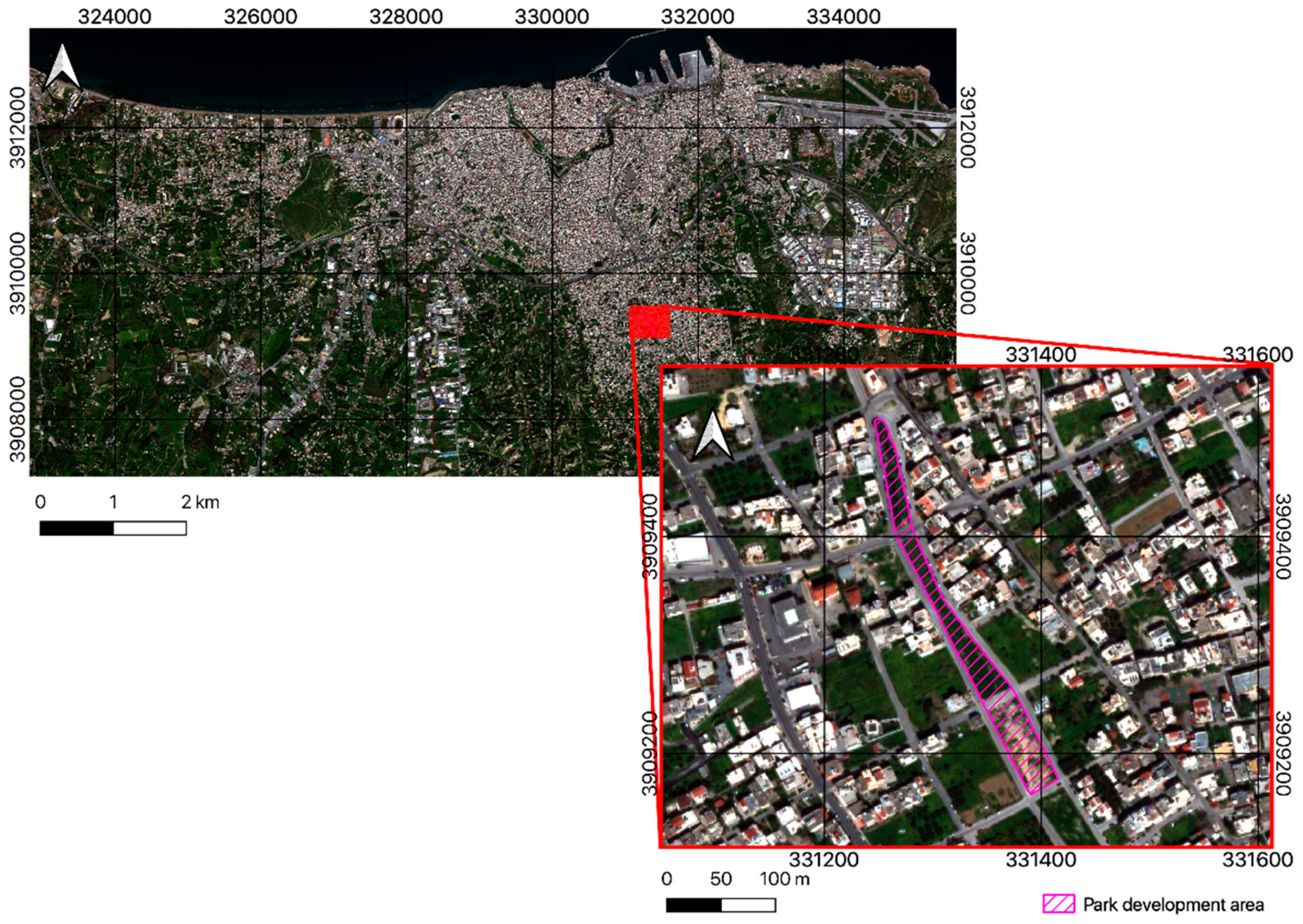
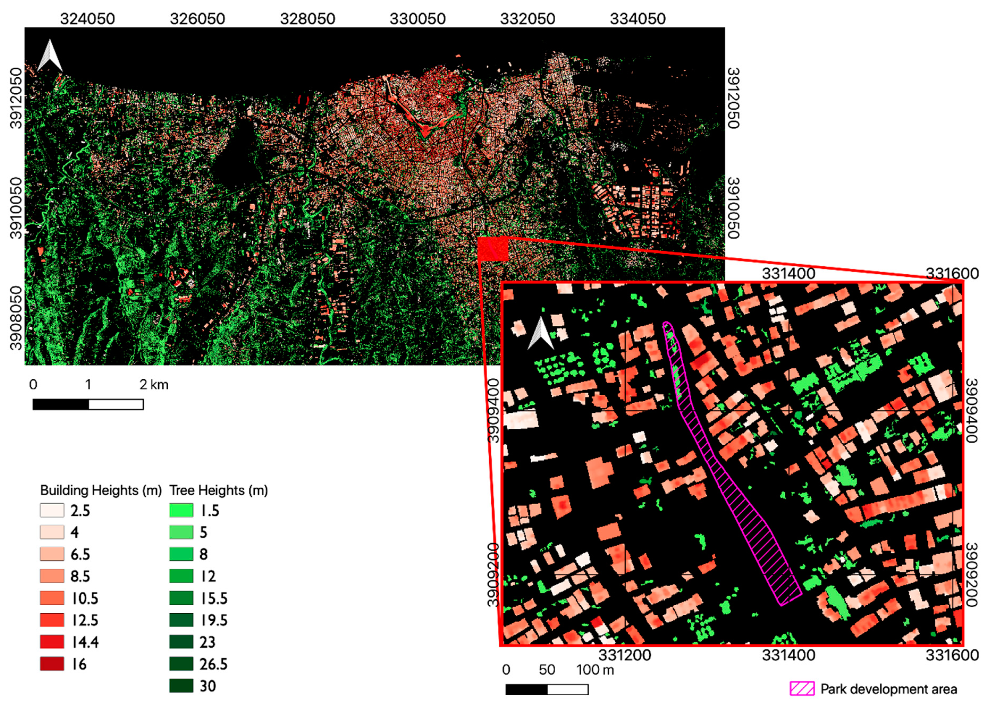
2.1. Study Area

This study focuses on the development plan for a new recreation park in a residential area of the city of Heraklion, the largest city of the island of Crete, and the fourth largest in Greece, with a population of more than 200,000 inhabitants. The region’s climate is characterized as hot-summer Mediterranean, falling in to the Csa category in the Köppen climate classification scheme. The approximate area of the municipality of Heraklion is 244.6 km² and it is divided in a number of urban units as presented in the Supplementary Materials (Figure S1). The Area of Interest (AOI) in this project is located in the district of Mesabelies, one of the southernmost and peri-urban areas of Heraklion, which is developing rapidly. The municipal development plan for this district includes the renovation of an area without any current use to a recreational park, which will include a bicycle lane, a pedestrian walking route, and children’s playgrounds. The intervention is labeled as a green space development, including tree and lower shrub plantations throughout the whole area. However, the respective development plan also includes the substitution of grass and bare soil with paved surfaces (bicycle and pedestrian lane). The first part of the development corresponds to a total area of approximately 1.5 hectares, about half of which are going to be part of the green space and are presented in Figure 1. The detailed development plan is presented in Section 2.3.1.

2.2. Model Requirements

SUEWS is a USM known for its simplicity which simulates the energy and water balance exchanges mainly for urban areas using commonly used spatial, meteorological, and census data [25,26,27]. The applicable scale of the model ranges from 10² to 10⁴ m, i.e., neighborhood scale [20]. The model is built upon the UEB equation (Equation (1)) [28], which is the main focus of this study, computing all of its components, as well as the urban water balance [29].

$$\mathrm{Q}*+{\mathrm{Q}}_{\mathrm{F}}={\mathrm{Q}}_{\mathrm{H}}+{\mathrm{Q}}_{\mathrm{E}}+\mathsf{\Delta }{\mathrm{Q}}_{\mathrm{S}}\left[\mathrm{W}{\mathrm{m}}^{-2}\right]$$

(1)

Q* represents the net all-wave radiation, Q_F the anthropogenic heat flux, Q_H the turbulent sensible heat flux, Q_E the turbulent latent heat flux, and ΔQ_S the net change in heat storage. Essentially, the left part of Equation (1) represents the energy inputs which are assumed to be distributed among the processes represented by the right part flux components, i.e., air heating (Q_H), water evaporation (Q_E), and energy being stored in elements of the urban environment (impervious materials, buildings) (ΔQ_S)_. Each of the UEB components is simulated based on a number of sub-models. These include the Net All-Wave Radiation Parameterization (NARP) [30] for the computation of Q* and the Objective Hysteresis Model (OHM) [31] for ΔQ_S, while evaporation and the surface conductance which are the basis for Q_E computation, are based on an adapted Penman–Monteith equation [32] and the methodology proposed by Jarvis [33], respectively. Q_F is computed using the Järvi et al. (2011) [25] approach, which is based on heating and cooling degree days and population density. Finally, Q_H is computed as the residual. This approach inevitably causes error propagation from all other flux components to the sensible heat flux component [25].

The architecture of SUEWS has been developed with a minimal input requirements approach. As of yet, the urban surface cover scheme implemented within the model consists of seven classes, namely paved, buildings, evergreen trees, deciduous trees, grass, bare soil, and water. Various characteristics of these surfaces such as albedo, emissivity, and moisture storage capacity may be edited within the model to correspond to the area of implementation (

Table 1. Parameterization of surface cover classes, same as Panagiotakis et al. (2021) [16], Ward et al. (2016) [34].

Surface Type	Albedo	Emissivity	Storage Cap (mm)
Paved	0.12	0.95	0.48
Buildings	0.15	0.91	0.25
Evergreen Trees	0.1	0.98	1.3
Deciduous Trees	0.12–0.18	0.98	0.3–0.8
Grass	0.18–0.21	0.93	1.9
Bare Soil	0.21	0.94	1
Water	0.1	0.95	0.5

). Other urban form parameters required include the mean building and tree heights, while urban function inputs include human behavior information such as energy and water use, and population density. The minimum meteorological data requirements are: incoming shortwave or solar radiation (K↓), air temperature (Tair), relative humidity (RH), barometric pressure (p), wind speed (U), and precipitation (P). An in-depth analysis of the model functionality is presented by Järvi et al. (2011,2014) [25,26].

Several studies have assessed the performance of the model in a variety of urban typologies and climates [16,19,25,26,34,35]. This is predominantly achieved by exploiting EC observations of the turbulent fluxes in specific sites where such equipment is available and comparing the measurements with the model outputs. Naturally, the evaluation process is spatially restricted and corresponds to the source area of the flux tower. The evaluation results for the net all-wave radiation and the turbulent heat fluxes from such studies are presented in

Table 2. SUEWS evaluation results for net all-wave radiation, turbulent latent, and sensible heat flux for different sites. Text in brackets indicates the code name for a specific site/experiment as presented by the authors in the literature. RMSE stands for Root Mean Square Error.

City	Site Description	Q*		QE		QH		Reference
		R2	RMSE	R2	RMSE	R2	RMSE
Los Angeles (USA)	–	–	164.2 (Ar93)	–	53.6 (Ar94)	–	83.1 (Ar94)	Järvi et al., 2011 [25]
Vancouver (Canada)	–	0.95	44.9	0.74	32.5	0.77	39.1	Järvi et al., 2011 [25]
London (UK)	dense urban	0.988	17.76	0.245	24.66	0.528	47.1	Ward et al., 2016 [34]
Swindon (UK)	residential suburban	0.995	13.85	0.721	22.62	0.789	28.21	Ward et al., 2016 [34]
Shanghai (China)	central business district	–	–	0.19 (QF,S Irr)	16.9 (QF,S Irr)	0.57 (QF,0 Noirr)	42.6 (QF,0 Noirr)	Ao et al., 2018 [19]
Helsinki (Finland)	–	0.74 (He2)	29.3 (He2)	0.48 (He2)	4.1 (He2)	0.74 (He1)	28.2 (He1)	Järvi et al., 2014 [26]
Basel (Switzerland)	–	0.99 (BSPR)	16.2 (BSPR)	−0.11 (BSPA)	0.8 (BSPA)	0.91 (BSPR)	42.1 (BSPR)	Järvi et al., 2014 [26]
Montreal (Canada)	–	0.89 (PR)	36.8 (PR)	0.59 (RL)	7.2 (RL)	0.86 (PR)	30.7 (PR)	Järvi et al., 2014 [26]
Minneapolis-Saint Paul (USA)	–	0.98 (SP2)	36.1 (SP2)	0.48 (SP2)	3.7 (SP2)	0.82 (SP1)	28.2 (SP1)	Järvi et al., 2014 [26]
Dublin (Ireland)	Mix of dense commercial units and residential apartments	–	–	0.11	9.98	0.67	24.65	Alexander et al., 2016 [35]
Hamburg (Germany)	West: large warehousing Units East: green vegetation, trees and little building coverage	–	–	0.45	37.72	0.56	32.07	Alexander et al., 2016 [35]
Melbourne (Australia)	Medium-density residential houses 5–8 m tall, open spacing and an ample amount of vegetation	–	–	0.06	30.99	0.25	31.77	Alexander et al., 2016 [35]
Phoenix (USA)	Low-rise residential housing 5–8 m tall with dry xeric landscaping	–	–	0.00	7.99	0.67	43.59	Alexander et al., 2016 [35]
Heraklion (Greece)	Commercial area: mix of low and mid-rise buildings	0.99	54	–	–	0.85	61.36	Panagiotakis et al., 2021 [16]

below. These are indicative of the model performance, highlighting the need for site-specific parameterization.

It should be noted that the results presented here are the best reported in each case study, which in most cases, included a number of different experiments to improve the model performance, or even different test sites within a city. Where available, the names of the different test sites/different experiments are presented in Table 2 in brackets.

For the net all-wave radiation Q*, Ward et al. [34] reported the lowest RMSE reaching 13.85 W m⁻² in Swindon (UK), in the case where observed longwave radiation (L↓) is provided in the forcing data as input for the model. In turn, Järvi et al. [26] presented RMSE values as low as 0.8 W m⁻² in Basel for the BSPR site, and finally, Alexander et al. [35] reported an RMSE of 24.65 W m⁻² when comparing modeled vs. observed sensible heat flux in Dublin (Ireland). In all, latent heat flux obtains the lowest RMSE values. However, this is directly related to the maximum and minimum values generally observed for each flux component, which vary significantly. For example, the net all-wave radiation values are inherently larger than the respective of the latent heat flux; hence the corresponding errors should be interpreted accordingly. Accounting for model performance in different regions and applications should be done with care, due to the inability to generalize the results across different sites exposed to different forcing data and/or varying typologies. However, in cities where the model performance has been assessed, as in our case by Panagiotakis et al. (2021) [16], and in the same wavelength as previous studies [17], a solid basis for interpretation of model outputs for this region is available.

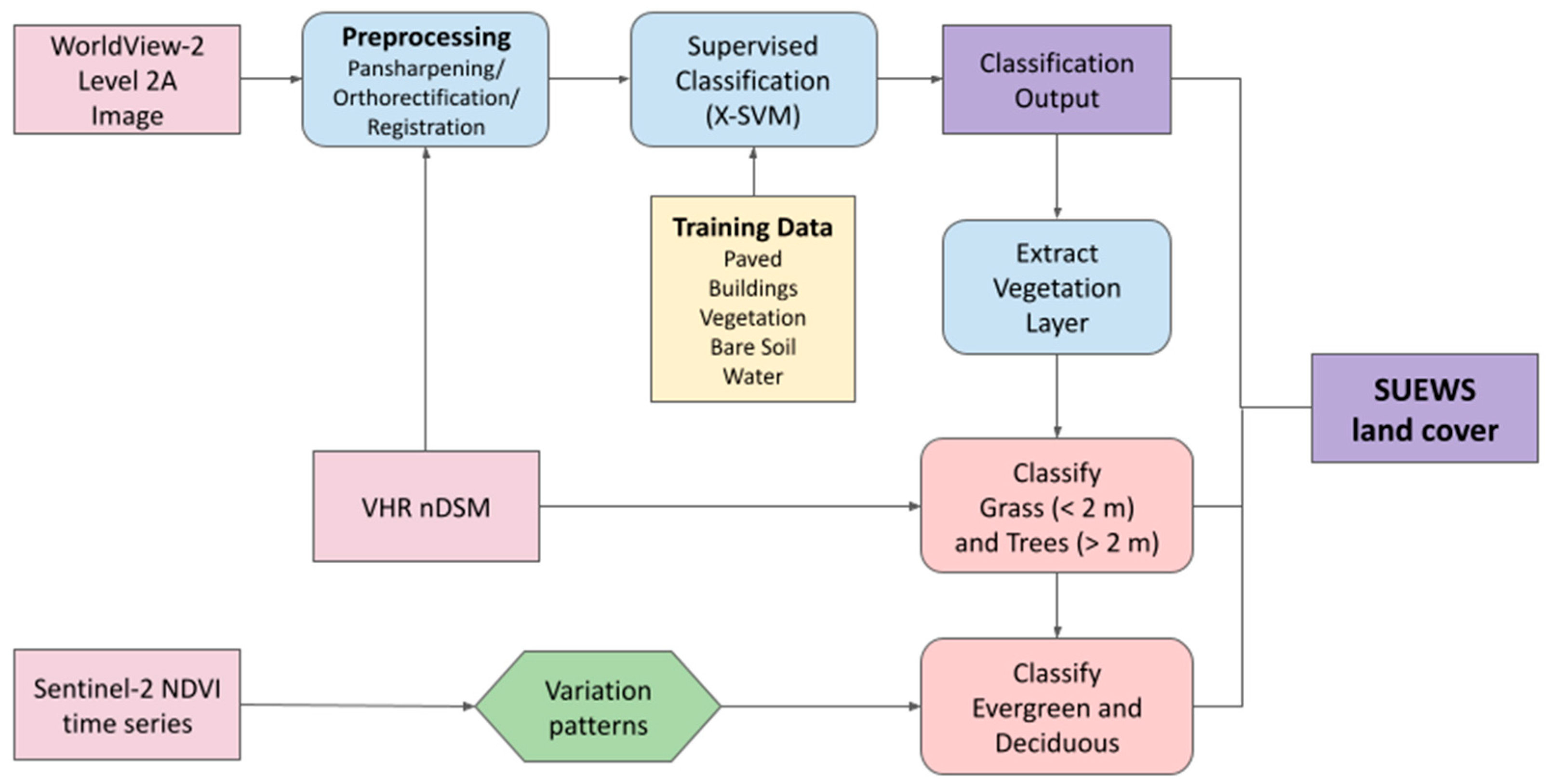
2.3. Data Preparation Workflow

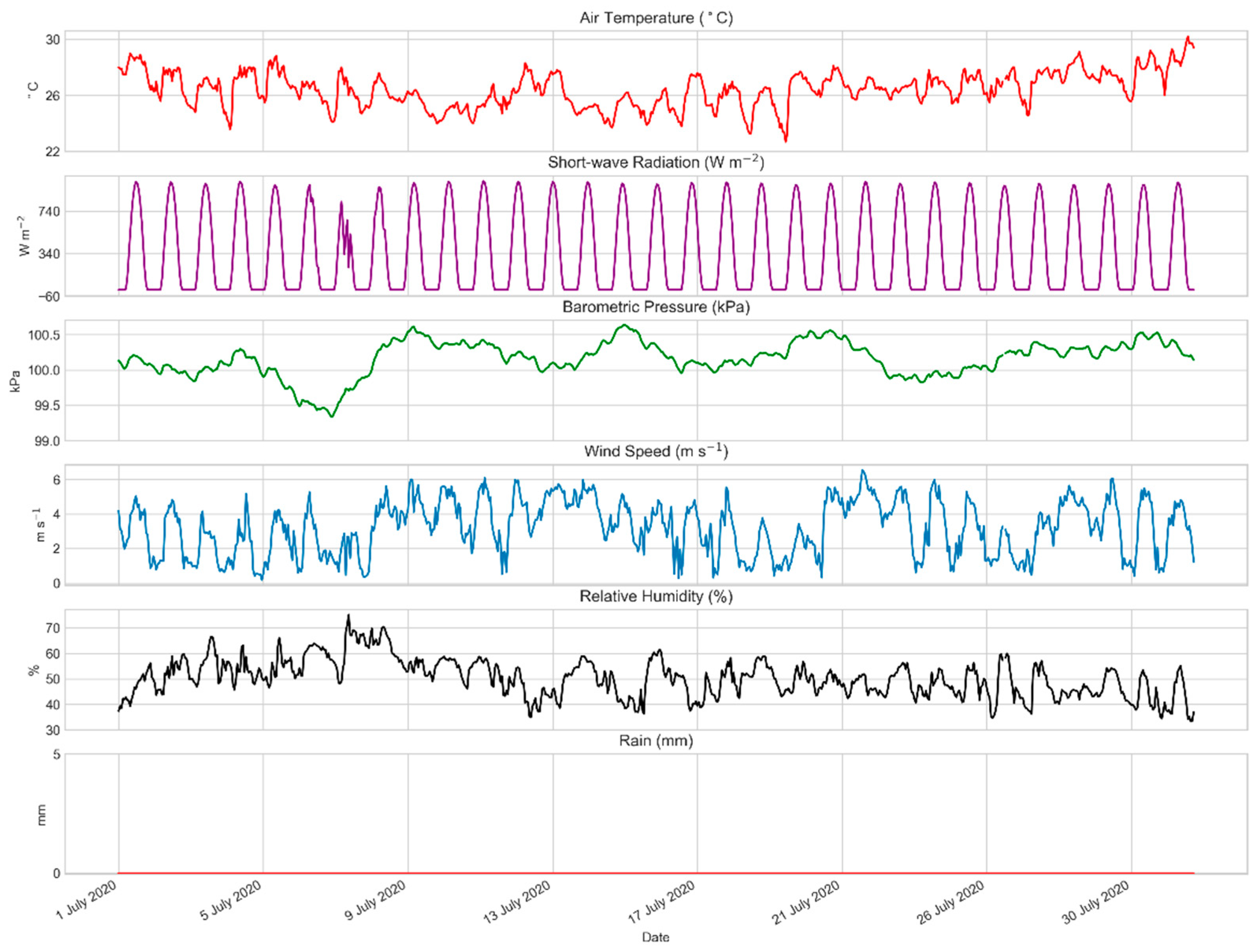
As described by Ward et al. [27], SUEWS requires input parameters related to the urban surface cover and morphology presented in

Table 3. Spatial data requirements for SUEWS [27].

Type	Definition	Reference/Comments
	Building/Tree Morphology
Mean height of building/trees	Mean height of objects (m above ground level (agl)).	[31]
Frontal area index	Area of the front face of a roughness element exposed to the wind relative to the plan area.	[31]
Plan area index	Area of the roughness elements relative to the total plan area.	[31]
	Land cover fraction	Should sum to 1
Paved	Roads, sidewalks, parking lots, impervious surfaces that are not buildings.	-
Buildings	Buildings.	Same as the plan area index of buildings in the morphology section.
Evergreen trees	Trees/shrubs that retain their leaves/needles all year round.	Tree plan area index will be the sum of evergreen and deciduous area. Note: same as the plan area index of vegetation in the morphology section.
Deciduous trees	Trees/shrubs that lose their leaves.	Same as above.
Grass	Grass.	–
Bare soil	Bare soil—non vegetated but water can infiltrate.	–
Water	Rivers, lakes, ponds, swimming pools, fountains.	–

below, which can be derived using a very high-resolution land cover map along with a normalized Digital Surface Model (DSM). In the following section, the process of producing this information is described in detail.

The workflow for producing the surface cover map using multi-source EO data is presented in Figure 2. WorldView-2 (WV2), very high spatial resolution imagery which was acquired on 19/03/2020 was used to produce the baseline surface cover map. WV2 imagery contains a panchromatic, at 0.5 m × 0.5 m, and 8 multispectral bands, at 2 m × 2 m (Table S1). The processing of this product includes radiometric and sensor-related corrections, providing a Circular Error (CE90) ranging from 5 m to 23 m. As shown in Table 3, SUEWS input requirements include 3 vegetation classes, namely Grass, Evergreen Trees, and Deciduous Trees. Extracting these solely from WV2 imagery is not possible due to vegetation spectral similarity in the available bands. In order to overcome this issue, we exploit a high resolution normalized DSM (nDSM, Figure S2) to discriminate between grass and trees, as well as time series of Sentinel-2 imagery (20 × 20 m, Table S2) downscaled to 10 × 10 m [36] to categorize trees as evergreen and deciduous.

Orthorectification is a fundamental preprocessing step, because satellite images inherently come with geometric distortions [37], related sensor, and target conditions, including topography. WV2 orthorectification was based on Rational Polynomial Coefficients (RPC) model [38], which was used in conjunction with a very high resolution DSM (posting 1 m × 1 m) for the city of Heraklion [39]. Pansharpening of the initial WV2 image improves the resolution of the final result to 0.5 × 0.5 m, preserving the original radiometry. This process was based on the Hyperspherical Color Space Resolution Merge algorithm [40]. Optimization of the orthorectified product was achieved with a follow-up registration algorithm. The ‘Georeferencer GDAL’ plugin of QGIS [41] was used to register the product, using the Thin Plate Spline transformation and the Lanczos resampling method which provided the best results in combination with 11 Ground Control Points (GCPs) (Figure S3). Google Maps was used as the GCPs reference, due to the ease of access and the satisfactory co-registration of this layer with the already existing data (i.e., the DSM used). The minimum distance between the GCPs was 1500 m corresponding to 1/10th of the diagonal distance of the image. To evaluate the final product, 21 check points equally distributed across the area of interest were used from the same reference as the GCPs (Figure S3). A minimum distance of 500 m was ensured from the latter, to avoid spatial autocorrelation and the introduction of bias in the validation process. The result added up to RMSEr = 0.9 m and the 95% interval circular error RMSE_CL95 = 1.56 m, a significant accuracy improvement.

Following, to map the surface cover, the final orthorectified product was classified, using also the Normalized Difference Vegetation Index (NDVI), extracted from WV2 red and near infrared bands (Table S1) as an extra spectral band. A recent extension of the traditional support vector classifier (SVM), namely X-SVM [42] was used. The X-SVM classifier reduces the need for manual parameterization of the classification process, assisting the user to reach optimum results much faster. To produce the surface cover map, 9 classes are originally selected and a minimum number of 50 training points for each class is acquired from the original WV2 image. Some classes are merged, after the classification of the image is executed. This approach is standard when working with classes which are not inherently separable from the spectral signatures of the objects in the image, i.e., buildings which may include roofs with tile, cement or insulation material. Indicative locations of the respective sampling points in the vicinity of the urban intervention are shown in Figure 3.

The product of the X-SVM-based classification is a surface cover map containing the following five classes: Paved, Buildings, Vegetation, Bare Soil, and Water. In order to fine tune the classifier parameters, 100 random reference points per class were selected from the original satellite image and were used to iteratively evaluate the classification outputs. Then, the optimum classification product was selected based on the overall classification accuracy, reaching the maximum value of 89.9%. To improve the classification outcome, a smoothing filter was used to remove pixel clusters smaller than 5 pixels, assigning values based on the surrounding pixels’ values. This step diminishes the salt and pepper effect often encountered in pixel-wise classification outputs which may be caused by high local spatial heterogeneity between neighboring pixels [43]. Finally, spatial masks were used, derived from in-house available polygons, to improve the result of the classification regarding buildings, and the road network. Using the aforementioned evaluation methodology, the overall accuracy of the final product was found at 92.6% (the respective confusion matrix is given in Table S3).

The approach for differentiating grass and trees is straightforward and easy to implement when an nDSM is available. The latter is a raster which includes only the absolute heights of 3D objects on the surface of the area, i.e., buildings, high vegetation, etc. By extracting vegetation as a layer from the classified image and applying it as a mask on the nDSM, we can then set a threshold of 2 m to classify the vegetation layer. An indicative overlay of the two layers is presented in Figure S4. All pixels with values above the threshold are classified as trees, whereas the ones falling below the threshold are considered to be grass.

With the vegetation layer split into the subcategories of grass and trees, the latter was subsequently processed to separate evergreen from deciduous trees. The approach to do this involves the assumption that seasonal variations in NDVI values are expected to differ between the two classes, as deciduous trees seasonally shed their leaves, usually in autumn. This difference in phenological state is expected to be evident when analyzing time series of satellite data. The time interval selected is the whole year of 2020, and the Sentinel-2 data are filtered with a maximum cloud fraction threshold of 10%. Cloud and cloud shadow masking were conducted using the Sentinel-2 cloud probability band, setting the cloud probability to less than 5%, and masking out values classified as cloud shadow or cirrus in the scene classification band (SCI). The resulting image collection consists of 63 images. In the case of Sentinel-2, NDVI corresponds to the normalized difference between bands B8 and B4. Yearly NDVI statistics (min and max values) were used to evaluate the variations which are attributed to the phenological state of vegetation, and discriminate evergreen and deciduous trees, as per Chrysoulakis et al. [13]. The minimum and maximum NDVI images were initially masked, using the high vegetation layer produced previously, and the pixels of the latter were classified as evergreen or deciduous, based on NDVI thresholds from the literature, presented in

Table 4. NDVI thresholds for separating evergreen and deciduous trees adapted from Chrysoulakis et al. (2018) [13].

Vegetation Type	NDVI min	NDVI max
Evergreen	0.2	0.7
Deciduous	0.45	0.9

[13,39]. The deciduous and evergreen trees’ layers, as all the rest, retain the resolution of the pansharpened WV2 image, i.e., 0.5 m.

To extract the building and tree heights, we conduct a simple masking process using the buildings, evergreen trees, and deciduous trees’ layers from the finalized classified image, and the nDSM available superimposition of the buildings and the nDSM raster are presented in Figure S5. The masking process resulted in two raster-type maps with height information for each of the abovementioned layers, which are in turn used to compute the morphometric parameters required by SUEWS by employing a morphometric calculator included in the Urban Multi-scale Environmental Predictor (UMEP) [44].

The minimum meteorological and radiation input requirements of the USM (see Model requirements) were provided by the HECKOR flux tower [45], which is located close to the study area. Focusing on heat stress, the model ran for June and July of 2020. HECKOR observations for July are shown in Figure 4, whereas June was used as a spin-up period for the model, which essentially secures that the initial conditions, such as soil moisture, are based on model computations. Generally, Figure 4 indicates a typical dry summer month with overall high temperatures.

Finally, population density data, used to compute the anthropogenic heat flux in SUEWS, was provided by the National Statistical Service (census data). The mean population density for the city of Heraklion was used as input for the model (57 ha⁻¹).

2.3.1. Model Runs

This study aims at quantitatively analyzing the potential effects from the renovation of a new park in a residential area of Heraklion, and the surface cover changes modeled in this study are based on the development plan, as provided by the Heraklion Municipal Authorities (Municipality of Heraklion 2021; personal communication). Therefore, the baseline model run simulated the current situation of the study area, whilst a second run simulated the scheduled surface cover changes as depicted in the surface cover maps shown in Figure 5. As mentioned earlier, the imminent changes include the plantation of several trees in the perimeter of the park, and the substitution of bare soil/vegetated surfaces with pavements which will serve as pedestrian routes and bicycle lanes. The model ran by using a grid configuration with 100 m × 100 m cells covering the urban intervention area, as well as the surrounding building blocks (Figure 6). The model outcomes for each grid cell were analyzed on the basis of the corresponding surface cover change.

The area is residential, and the major Local Climate Zone (LCZ) type is LCZ6 [46] corresponding to Open Low-Rise based on the classification scheme proposed by Steward and Oke [47]. Numerous patches of land of no particular use exist, which are mostly covered by low vegetation or bare soil.

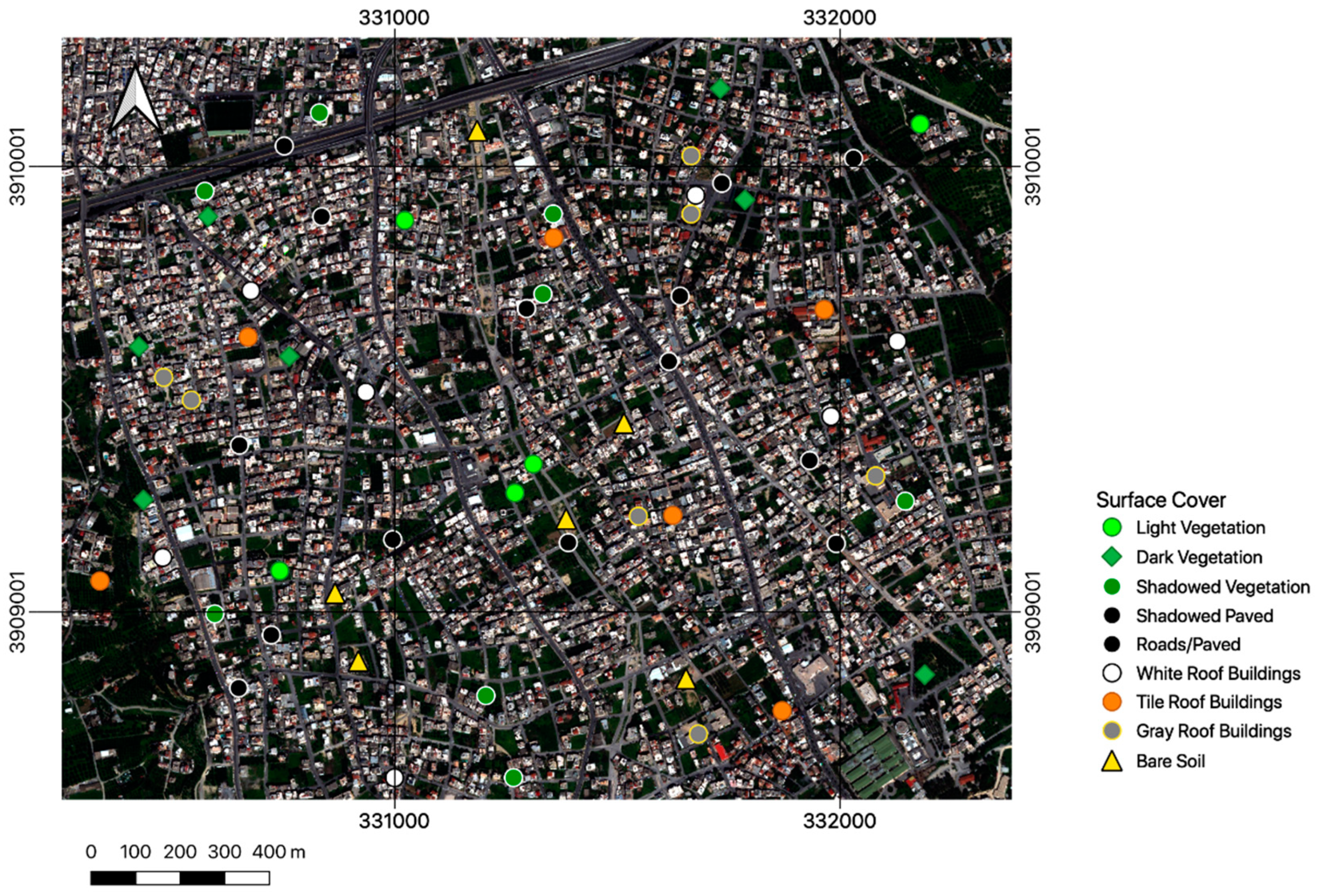
2.3.2. Uncertainty Analysis

Generally, model outputs can only be as good as the model inputs, following the garbage in, garbage out principle. In this context, it is important to assess how the outputs of the model are affected by the accuracy of the spatial data inputs. This is done by conducting a sensitivity analysis of the model with respect to the surface cover fractions and the surface cover classes’ precision (Table S4). The overall process (Figure S3) involves conducting a baseline model run, using the surface cover fractions for each grid cell as computed by the standard process of zonal statistics, and a second run using different land cover fractions which are computed as:

$$F_i^{true}=f_i\ast p_i+R\ast \overline{f_i}$$

(2)

where f_i is the initial land cover fraction of class i, p_i is the class-wise precision, R is defined as the residual as in:

$$R=1-{\displaystyle \sum }_i^n{f}_i\ast p_i$$

(3)

and finally, $\overline{f_i}$ is the mean value of the fraction for class i across all grid cells. These equations are designed so as to account for the class-wise uncertainty of the surface cover maps and the characteristics of the area (i.e., the mean fraction values for class). Hence, comparing the model outputs of the baseline and the second model run with the edited surface cover fractions, an estimation can be made regarding the potential uncertainty in the mean flux values computed by the model, i.e., ΔQ*, ΔQ_E, ΔQ_H, ΔQ_F and Δ(ΔQ_S).

3. Results

The surface cover map corresponding to the 5-class classification scheme, with an overall accuracy of 92.6%, is presented in Figure 7. As described in detail in the previous section, the vegetation layer is extracted and categorized as grass and trees using the nDSM, and in turn, split into the classes of Grass, Deciduous and Evergreen trees. The minimum and maximum NDVI maps from Sentinel-2, used to discriminate the tree classes are shown in Figure S7. The final land cover map of the vicinity of the development area is shown in Figure 8. The accuracy of the latter reaches 89.6% and the confusion matrix with the corresponding class-wise accuracies is displayed in Table S4.

The surface cover map is combined with the grid covering the intervention area to estimate the current and future cover fractions for each grid cell. The resulting land cover percentages are presented in Figure 9, along with the percentage changes (future-current) per class and per grid cell, shown in detail in Table S5 and Figure 10. It should be noted that grid cells 1, 2, 6, 7, 11, and 12 refer to the surrounding area of the AOI and are not going to undergo any changes in land cover. Hence, the changes presented in all tables henceforth, refer to the remaining grid cells which experience changes in land cover. The bulk albedo of each grid cell is also calculated using a weighted average of the fraction of each surface type within the grid and the corresponding albedo value (Table 1).

Paved cover shows a general increase in most grid cells, with a maximum increase of 8.9% for grid cell 9, as a result of the bicycle and pedestrian lane development. Evergreen trees do not show significant changes, with the exception of grid cell 10 with an increase of 2.6% in this class, due to the plantation of olive trees in this region of the park. The development plan includes the plantation of deciduous trees across the whole area of the park, hence this class percentage increases for all grids, with a maximum of 4.3% for grid cell 9. Grass is the dominant land cover class of the area prior to the development, and it is mainly substituted with paved and tree cover, showing an overall decrease across all grids, with the exception of grid cell 10 which shows an increase of 2.8%. Likewise, bare soil is mainly substituted with paved cover, trees, and grass, showing decreasing trends in all grid cells, with a maximum of −11.9%.

The building and tree height layers extracted from the nDSM and the land cover map are presented in Figure 11, and these layers are used to compute the morphometric parameters for buildings and trees for the same grid configuration and for the current as well as future scenarios. Buildings are not affected in any way by the development plan and consequently, the morphometric parameters presented in Table S6 are not subject to change. It should be noted that the computed Plan Area Index and Mean Building Height for the grid cells are in line with the LCZ6 category as reported by Mitraka et al. [46], with the exception of grid cell 9 and 10 where there is an absence of buildings. On the other hand, as shown in Figure 5, a number of trees will be planted in the development area; hence, the corresponding morphometric parameters are affected (Table S7). The changes in mean vegetation height are caused by the fact that in the modeling process, the height of the new trees is assigned at 2.5 m to simulate the early years of growth. This tends to lower the overall mean tree height in the grid cells where trees are already present, and increase the mean height in grid cells with few or no trees at all. The roughness length follows the corresponding decrease or increase in approximately 1/10th of the surface elements’ mean height, which in this case are the trees.

The uncertainty introduced by the class-wise precision of the surface cover map used to compute the surface cover fractions for each grid cell is presented in

Table 5. Absolute mean flux differences per grid (baseline-error model run).

Grid Cell	ΔQ* (W m−2)	ΔQF (W m−2)	Δ(ΔQS) (W m−2)	ΔQE (W m−2)	ΔQH (W m−2)
3	0.62	0.00	2.89	0.13	2.14
4	0.48	0.00	2.67	0.17	2.03
5	0.33	0.00	0.96	0.18	0.45
8	0.37	0.00	1.66	0.00	1.28
9	0.16	0.00	0.10	0.21	0.05
10	0.36	0.00	0.60	0.30	0.06
13	0.47	0.00	1.34	0.03	0.84

as absolute mean value differences. These are later on used to interpret the model outputs, which are assumed to include the values shown in Table 5 as uncertainties in the overall means, per flux component and per grid cell.

The simulations of the model (baseline and future development scenario) are presented and discussed with regard to the observed differences in the urban surface fluxes. The grid cells which do not experience any changes in surface cover do not show any differences in the outputs of these two model runs, as expected based on the mechanics of the model, which essentially runs for each cell individually. Naturally, this limitation which overlooks advection between neighboring cells, is taken into account in the interpretation of results, and in the case where large differences are observed in the results of a cell, the surrounding cells are also expected to be affected. Additionally, since there is no change in the Buildings plan area (no buildings are taken down, or built), and no change is introduced in the population density, the anthropogenic heat flux component, which is indicative of urban function, does not show any changes and is hence omitted from the following tables and figures.

Table 6. Model outputs of the current and future runs per grid cell for Net All-Wave Radiation (Q*), Sensible Heat Flux (Q_H), Latent Heat Flux (Q_E), and Net Change in Heat Storage (ΔQ_S). The table presents monthly (MM), daytime (DM), and nighttime (NM) mean values in W m⁻².

	Cell 3		Cell 4		Cell 5		Cell 8		Cell 9		Cell 10		Cell 13
	cur	fut	cur	fut	cur	fut	cur	fut	cur	fut	cur	fut	cur	fut
Q*
MM	223.5	224.3	221.6	223.1	215.3	215.3	221.9	221.9	215.4	218.5	213.3	215.3	222.7	222.7
DM	421.8	423.1	4186	421.2	407.7	407.6	418.9	419.0	408.0	413.3	404.4	407.9	420.4	420.4
NM	−44.7	−44.8	−44.8	−44.9	−44.8	−44.8	−44.6	−44.6	−45.0	−45.1	−45.2	−45.2	−39.9	−39.9
QH
MM	150.0	150.0	151.4	149.6	175.2	175.9	156.8	157.2	170.4	164.7	174.9	175.1	159.5	160.2
DM	238.2	238.1	241.2	237.2	291.2	292.7	251.6	252.4	281.1	269.2	289.0	290.0	257.8	259.1
NM	28. 8	29.1	28.1	29.3	16.7	16.4	26.7	26.6	19.1	21.7	19.0	18.2	31.2	31.2
QE
MM	7. 9	7.4	7.6	7.07	4.3	4.2	6.9	6.7	4.4	5.0	3.0	3.0	7.2	6.6
DM	11.4	10.5	10.8	10.0	5.5	5.2	9.7	9.4	5.5	6.6	3.2	3.2	10.3	9.3
NM	3.3	3.2	3.3	3.2	2.7	2.7	3.1	3.1	2.8	2.8	2.6	2.5	3.1	3.0
ΔQS
MM	88.1	89.3	84.9	88.9	58.0	57.4	80.4	80.3	62.9	71.0	57.6	59.4	78.1	78.0
DM	199.1	201.5	193.6	201.0	138.0	136.7	184.6	184.2	148.4	164.5	139.1	141.7	179.2	178.9
NM	−61.4	−61.7	−61.4	−61.9	−49.4	−49.0	−59.6	−59.5	−52.1	−54.8	−51.9	−51.2	−58.2	−58.1

and Figure 12, Figures S8 and S9 sum up the outputs of the baseline and future development model runs, which are displayed in terms of percentages, raw values and overall, daytime, nighttime, and hourly mean values.

4. Discussion

Overall, the methodology presented in Figure 2 using multi-source EO data manages to capture urban form accurately for the purposes of parameterization of the USM. One of the major challenges of this approach is the need for adequate co-registration of the VHR products used to extract building and tree heights, which in our case, is achieved with the use of registration algorithms. The NDVI threshold process mentioned in the Materials and Methods section is an important source of error of the surface cover map, something that is evident from the class-wise precisions of the Evergreen and Deciduous Trees classes (Table S4). A future development of this methodology will account for the potential below crown surface cover which may include grass, paved cover, and bare soil surfaces, and is expected to affect the NDVI values computed. Moreover, paved surfaces are, in part, erroneously misclassified as buildings and bare soil, lowering the class precision. This is attributed to the spectral similarity often encountered in pixels of these classes, which makes them indistinguishable to the classification algorithm. Even so, the final land cover map produced to match the desired classification scheme including the 3 vegetation classes, presented in Figure 8, shows very good accuracy.

In turn, the model outputs for the baseline and future runs provide insight regarding the UEB response to the land cover changes expected to take place. Figure 12 presents these land cover changes in terms of percentages along with the modeled changes in the UEB components.

Regarding grid cell 3, the bulk albedo decreases from 0.13 to 0.12 (Table S5), whilst emissivity increases, since grass and bare soil are replaced by materials with higher emissivity values, resulting in a small increase of the net all-wave radiation Q*. As a general rule, changes in albedo propagate to the outgoing components of the shortwave radiation, consequently affecting the Q*. The increase of paved cover for grid cell 3 is evident from the observed differences regarding the net change in heat storage ΔQ_S which increases when impervious cover is expanded. This leads to the storage of heat during the daytime which is released during the night, forcing the air temperature increase. A notable observation regards the generally low values of Q_E. This can be attributed to the reduced evaporation taking place, since soil moisture is not replaced through rainfall during the study time interval. Grass, bare soil and evergreen trees have the largest storage capacity values as presented in Table 1. Since these classes are replaced, the overall storage capacity of the grid becomes lower and this leads to changes in the Soil Moisture Deficit (henceforth SMD), which is greater in the future land cover scenario (Figure S9). This gap tends to fade out as the total change in soil and surface moisture stores becomes smaller, hence diminishing the differences in Q_E. In SUEWS, Q_H is computed as the residual, so its values are very responsive to the changes in the rest of the energy fluxes computed by the model; the results for grid cell 3 highlight this behavior. In the early days of the month, when Q_E shows larger differences, Q_H increases to account for the increase in Q* and ΔQ_S, and the decrease of Q_E. As time passes and Q_E differences fade out, Q_H starts to decrease to restore the energy balance. The changes mentioned in Q* and ΔQ_S seem to peak during the time that the maximum values of these quantities are observed, i.e., close to midday, while Q_E differences are most evident early in the morning.

The changes in land cover for grid cell 4 are similar to grid cell 3, with the exception of the increase in paved surfaces, which is higher in grid cell 4 replacing grass and bare soil. This leads to a greater increase of ΔQ_S, which shows an overall mean increase of 4 W m⁻² peaking at midday, reaching maximum differences just over 10 W m⁻². In this grid cell, the bulk albedo does not change, so the changes in Q* values are mostly attributed to changes in emissivity. In the same wavelength as before, the model outputs show differences in Q_E, which become lower over time. To counterbalance the increase of ΔQ_S, Q*, and the fading decrease of Q_E, Q_H decreases with the differences between the future scenario and the baseline run outputs becoming larger over time and reaching differences up to −8.83 W m⁻² (future-baseline). The same pattern is observed in the total surface and soil moisture stores, and the SMD (Figure S9). These results indicate that when it comes to Q_E, which is seemingly a driving force in UEB for the model runs conducted, the differences observed caused by the changes in surface cover seem to fade out in time.

This is partially related to the forcing data, i.e., the local climate in general, as well as the absence of rain, and most importantly, on the state of the vegetation and the soil moisture which gradually reduces, leading to dry soils, with high SMD values and increased surface conductance. Given the dry summer period of study, which is typical for this type of Mediterranean climate, this is expected to be standard for this area. As pointed out by Järvi et al. [25], the surface conductance parameters play a major role in how efficiently water is exchanged between the vegetation layers and the atmosphere. Hence, soil dryness significantly affects the latent heat flux Q_E. Essentially, dry soils translate to a decrease in evaporation rates, due to soil moisture saturation, and since the latent heat flux is the latent heat of vaporization, it can only but follow this decrease. Such variations in Q_E may have significant effects on the UEB. Manoli et al. [48] have presented the effect of out-of-phase solar radiation and water availability which causes different hysteresis patterns of the surface urban heat island seasonality. This highlights the significance of evaporation in the urban climate. Given that no validation of the modeled Q_E based on observations has been conducted, conclusions regarding the potential underestimation of Q_E must be cautiously interpreted. A palette of parameters within the model may be edited to fine tune the outputs, like the surface conductance parameters, the irrigation patterns, and the threshold above which evaporation from a wet surface is considered to take place. The fine-tuning of these is expected to diminish the underestimation of evaporation which is estimated to take place, a conclusion based on the very low evaporation rates modeled, demoting the validity of the observed Q_E values.

Grid cell 5 shows minimal changes in surface cover, as only a very small proportion of the development area falls within the grid area. However, the change in fluxes is in line with the changes in surface cover and the results of the rest of the grid cells. A decrease of paved surfaces leads to a decrease in ΔQ_S peaking at midday. This, in conjunction with the pattern of Q_E, causes Q_H to obtain an increase, which becomes lower over time. The same can be concluded for cell 8, where the maximum surface cover change is observed for deciduous trees with an increase of 0.4%, while paved, grass and bare soil cover decreases. It is easily observed that the differences in values presented in Table 6 fall within the margins of error shown in Table 5 for cell 8 and 13. As expected, the flux difference trends are very similar to those of cell 5.

Grid cell 9 shows the largest differences in surface cover, reaching 8.9% for paved (increasing) and grass (decreasing) cover and, in that sense, it is likely to be the only cell subject to changes which will alter UEB in a small, but measurable amount. The reason that this does not apply to the previous grids, is the magnitude of the surface fluxes. This is evident by examining the values presented in Table 5 and Table 6 and the corresponding differences between model runs as in Figure 12 and Figure S8. Changes in Q* and ΔQ_S are approximately an order of magnitude lower than the modeled fluxes across these grids, hence are considered negligible. Grid cell 10 shows a significant decrease in bare soil cover. The decrease of albedo results in a small increase in Q*, and the increase of paved cover leads to an increase of ΔQ_S. It is interesting to note that despite the decrease of bare soil, which is the largest across all grids, Q_E remains largely unaffected. This behavior is directly related with the non-accurate extreme soil dryness which is simulated in the model runs; but still, this observation indicates that in cases of intense prolonged drought, changes in the bare soil fraction do not affect the evaporation rates. Notably, cells 9 and 10 are the only ones where the SMD decreases, based on the changes in surface cover. Cell 10 shows the largest differences as SMD decreases in the future scenario, an observation related to the increase in all vegetation classes’ fractions.

The maximum flux values modeled occur at near-midday, which is also the time that the maximum differences in the model runs are observed across all grid cells. These maxima reach 746.9 W m⁻² for Q*, 462.4 W m⁻² for Q_H, 22.2 W m⁻² for Q_E, and 309.7 W m⁻² for ΔQ_S (see Table S8) in the baseline model run for grid cell 9. Comparing these values with the variations shown in Figure S8, which correspond to changes in mean values lower than 10%, leads to the conclusion that such differences are considered very small to account for measurable effects in the neighborhood-scale microclimate. The percentage differences in mean values per grid cell and per flux component are presented in

Table 7. Percentage changes in mean surface flux values per grid.

	Q*	ΔQS	QE	QH
Cell 3	0.3%	1.4%	−6.6%	0.1%
Cell 4	0.7%	4.7%	−6.7%	−1.2%
Cell 5	–	−1.1%	−3.7%	0.4%
Cell 8	–	−0.2%	−3.2%	0.3%
Cell 9	1.4%	12.1%	13.1%	−3.4%
Cell 10	0.9%	3.1%	−1.6%	0.1%
Cell 13	–	−0.1%	−8.9%	0.5%

(previously presented in Figure 12). The only notable variations are observed for ΔQ_S and Q_E for grid cell 9. However, the increase observed in ΔQ_S is considered a predictable observation, something that does not apply for Q_E, as mentioned earlier. Q_E is generally expected to obtain low values, based on the long, dry summer period which is standard for Heraklion and generally for areas with a hot-summer Mediterranean climate. Still, the model output values propose that nearly no evaporation is taking place, something that is partially proved wrong by examining the variations and relatively high values of the relative humidity from the forcing data used. This underestimation propagates to modeled Q_H.

In general, the model outputs presented so far highlight the sensitivity of the model to surface parameters. Q_E is very sensitive to surface conductance and, as presented in detail by Ao et al. [19], appropriate irrigation patterns may critically improve the validity of Q_E outputs. Accurately modeling the soil moisture is a decisive step in reaching realistic results for the turbulent heat fluxes. Moreover, when modeling the effects of such interventions, potential changes in irrigation patterns have to be taken into account as urban function changes. The optimization of all the model parameters related to the evaporation process is expected to improve the overall flux simulation outputs, and reproduce realistic results, especially for Q_H and Q_E. Nonetheless, the changes in fluxes that are observed are indicative of SUEWS’s functionality and provide a qualitative insight of the UEB complexity in a real-world scenario. Other studies have shown that increasing the vegetation fraction of an area at the cost of paved surfaces leads to important increase in Q_E and important decrease in Q_H [16,17]. Our results indicate that in such cases, this process can be disturbed by dryness of vegetation and soils, which causes Q_E to reach a threshold which in turn affects the way Q_H is modeled. Additionally, as also noted by Panagiotakis et al. [14], the largest changes in UEB components are observed in the daytime, peaking at midday. This is clearly depicted in Figure S8c and Table 6.

5. Conclusions

This study presents how EO can be used for assessing the climatic impacts of urban interventions, focusing on how the development of a park in a residential area of a typical Mediterranean city is able to modify UEB at local scale. A versatile methodology is followed, which allows for the extraction of urban form information of any city, given the availability of VHR satellite observations. The processing workflow presented highlights the capabilities of EO data to produce accurate information on surface cover, as well as the limitations and difficulties encountered when working with multi-source geospatial data. A significant note relates to information exchange between coarse-scale satellite data (Sentinel-1, Sentinel-2, Landsat missions etc.) and neighborhood-scale modeling processes. Exploiting the full potential of time series of satellite observations is still a challenge, as simplistic approaches such as the one presented in this study tend to introduce errors. Nonetheless, this constitutes a prominent extension of this study, which may include model runs for a longer period (i.e., yearly), using a dynamic land cover which will account for seasonal changes in vegetation based on observational rather than modeled data.

In summary, our results are in agreement with past studies and have shown that:

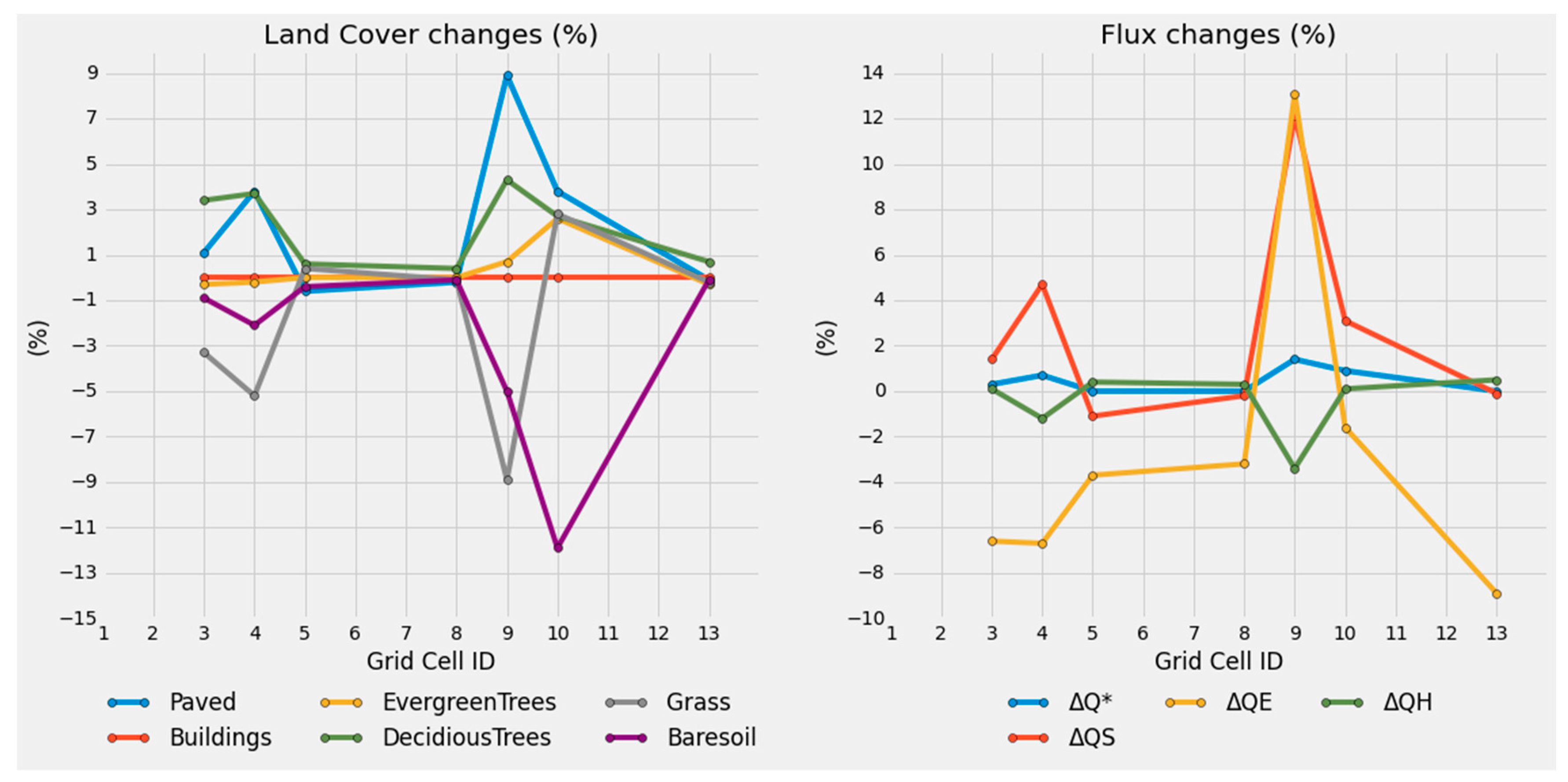
• In areas where the bulk albedo decreases due to substitution of vegetation with paved surfaces, Q* tends to increase. However, in this case study, the maximum increase of mean Q* reaches only 1.4%, and is hence considered not to have any significant effect on the neighborhood climate.
• In areas where impervious materials substitute pervious surfaces, ΔQ_S increases. This means more energy is ‘stored’ during the daytime, and is released at nighttime, hence reducing the standard nighttime temperature decrease. This is expected to occur in the development park, as paved cover is increased across most grid cells, at a magnitude that will not significantly alter the thermal comfort of the residents.
• All differences observed in the surface fluxes due to changes in surface cover show peaks during daytime. Q* and ΔQ_S differences peak at midday, while Q_E differences peak early in the morning. Q_H differences simply follow the result of these changes.
• Although Q_E was not realistically modeled, the observed trends still stand. This means that the pattern of substituting grass surfaces with paved cover and trees tends to lower the overall evaporation capability of the area, hence reducing Q_E and allowing for an increase in Q_H. As this is a rapidly developing area and more buildings are likely to be built in the near future, this trend is expected to increase.

Overall, in this case study, it is shown that imminent changes in surface cover at the fine scale are not expected to have a significant negative or positive effect in UEB, thus in air temperature, at the neighborhood scale. This is related to (a) the changes in surface cover are small; (b) the grid cells, which seemingly experience larger changes (i.e., increased paved cover) appear to also undergo changes which cancel out any significant effect (i.e., plantations of trees which partially make up for the overall vegetation percentage), and (c) the largest differences in mean flux values are observed for a spatially restricted fraction of the development area. However, it is evident that similar interventions at larger scales are likely to impact the neighborhood climate. This should be taken into account by urban planners and stakeholders in terms of the environmental component of sustainability as discussed by Chrysoulakis et al. [49], given that the Mediterranean region is likely to be a hotspot of global warming as temperatures are expected to rise faster around this region than globally over the next few decades [50].

Finally, the results of this study present a significant weakness in simulating Q_E because soil properties and the water availability of vegetation need to be more accurately parameterized. More detailed information on these parameters will be used in future studies.

References

1. United Nations, Department of Economic and Social Affairs, Population Division. World Population Prospects 2019: Highlights (ST/ESA/SER.A/423); Statistical Papers—United Nations (Ser. A), Population and Vital Statistics Report; United Nations: New York, NY, USA, 2019.
2. Meehl, G.A.; Tebaldi, C. More Intense, More Frequent, and Longer Lasting Heat Waves in the 21st Century; Science: New York, NY, USA, 2004; Volume 305, pp. 994–997. [Google Scholar] [CrossRef] [Green Version]
3. United Nations. Transforming Our World: The 2030 Agenda for Sustainable Development; UN Publishing: New York, NY, USA, 2015.
4. Caprotti, F.C.R. The New Urban Agenda: Key Opportunities and Challenges for Policy and Practice. Urban Res. Pract. 2017, 10, 367–378. [Google Scholar] [CrossRef] [Green Version]
5. Leichenko, R. Climate change and urban resilience. Curr. Opin. Environ. Sustain. 2011, 3, 164–168. [Google Scholar] [CrossRef]
6. Georgescu, M.; Morefield, P.E.; Bierwagen, B.G.; Weaver, C.P. Urban adaptation can roll back warming of emerging megapolitan regions. Proc. Natl. Acad. Sci. USA 2014, 111, 2909–2914. [Google Scholar] [CrossRef] [PubMed] [Green Version]
7. Synnefa, A.; Dandou, A.; Santamouris, M.; Tombrou-Tzella, M.; Soulakellis, N. On the Use of Cool Materials as a Heat Island Mitigation Strategy. J. Appl. Meteorol. Clim. 2008, 47, 2846–2856. [Google Scholar] [CrossRef]
8. Somarakis, G.; Stagakis, S.; Chrysoulakis, N. ThinkNature/Nature-Based Solutions Handbook; ThinkNature: Hague, The Netherlands, 2019. [Google Scholar] [CrossRef]
9. Marando, F.; Heris, M.P.; Zulian, G.; Udías, A.; Mentaschi, L.; Chrysoulakis, N.; Parastatidis, D.; Maes, J. Urban heat island mitigation by green infrastructure in European Functional Urban Areas. Sustain. Cities Soc. 2021, 77, 103564. [Google Scholar] [CrossRef]
10. Chrysoulakis, N.; Somarakis, G.; Stagakis, S.; Mitraka, Z.; Wong, M.-S.; Ho, H.-C. Monitoring and Evaluating Nature-Based Solutions Implementation in Urban Areas by Means of Earth Observation. Remote Sens. 2021, 13, 1503. [Google Scholar] [CrossRef]
11. Oke, T.R.; Mills, G.; Christen, A.; Voogt, J. Urban Climates; Cambridge University Press: Cambridge, UK, 2017. [Google Scholar] [CrossRef] [Green Version]
12. Oke, T.R. The urban energy balance. Prog. Phys. Geogr. 1988, 12, 471–508. [Google Scholar] [CrossRef]
13. Chrysoulakis, N.; Grimmond, S.; Feigenwinter, C.; Lindberg, F.; Gastellu-Etchegorry, J.P.; Marconcini, M.; Mitraka, Z.; Stagakis, S.; Crawford, B.; Olofson, F.; et al. Urban energy exchanges monitoring from space. Sci. Rep. 2018, 8, 1–8. [Google Scholar] [CrossRef] [Green Version]
14. Martins, T.A.; Adolphe, L.; Bonhomme, M.; Bonneaud, F.; Faraut, S.; Ginestet, S.; Michel, C.; Guyard, W. Impact of Urban Cool Island measures on outdoor climate and pedestrian comfort: Simulations for a new district of Toulouse, France. Sustain. Cities Soc. 2016, 26, 9–26. [Google Scholar] [CrossRef]
15. Fahed, J.; Kinab, E.; Ginestet, S.; Adolphe, L. Impact of urban heat island mitigation measures on microclimate and pedestrian comfort in a dense urban district of Lebanon. Sustain. Cities Soc. 2020, 61, 102375. [Google Scholar] [CrossRef]
16. Panagiotakis, E.; Kolokotsa, D.; Chrysoulakis, N. Evaluation of nature-based solutions implementation scenarios, using urban surface modelling. Green Energy Sustain. 2021, 1, 1–42. [Google Scholar] [CrossRef]
17. Ward, H.; Grimmond, C. Assessing the impact of changes in surface cover, human behaviour and climate on energy partitioning across Greater London. Landsc. Urban Plan. 2017, 165, 142–161. [Google Scholar] [CrossRef]
18. Ward, H.C.; Evans, J.G.; Grimmond, C.S.B. Multi-season eddy covariance observations of energy, water and carbon fluxes over a suburban area in Swindon, UK. Atmos. Chem. Phys. 2013, 13, 4645–4666. [Google Scholar] [CrossRef] [Green Version]
19. Ao, X.; Grimmond, C.S.B.; Ward, H.C.; Gabey, A.M.; Tan, J.; Yang, X.; Liu, D.; Zhi, X.; Liu, H.; Zhang, N. Evaluation of the Surface Urban Energy and Water Balance Scheme (SUEWS) at a Dense Urban Site in Shanghai: Sensitivity to Anthropogenic Heat and Irrigation. J. Hydrometeorol. 2019, 19, 1983–2005. [Google Scholar] [CrossRef]
20. Rafael, S.; Martins, H.; Marta-Almeida, M.; Sá, E.; Coelho, S.; Rocha, A.; Borrego, C.; Lopes, M. Quantification and mapping of urban fluxes under climate change: Application of WRF-SUEWS model to Greater Porto area (Portugal). Environ. Res. 2017, 155, 321–334. [Google Scholar] [CrossRef]
21. Taubenböck, H.; Esch, T.; Wurm, M.; Heldens, W.; Dech, S.W. From Earth Observation to Urban Planning in Cities. In Proceedings of the PLUREL Conference, Copenhagen, Denmark, 19–22 October 2010; pp. 1–6. [Google Scholar]
22. Xia, N.; Cheng, L.; Li, M. Mapping Urban Areas Using a Combination of Remote Sensing and Geolocation Data. Remote Sens. 2019, 11, 1470. [Google Scholar] [CrossRef] [Green Version]
23. Yu, W.; Zhou, W.; Dawa, Z.; Wang, J.; Qian, Y.; Wang, W. Quantifying Urban Vegetation Dynamics from a Process Perspective Using Temporally Dense Landsat Imagery. Remote Sens. 2021, 13, 3217. [Google Scholar] [CrossRef]
24. Sun, T.; Järvi, L.; Omidvar, H.; Theewues, N.; Lindberg, F.; Li, Z.; Grimmond, S. Urban-Meteorology-Reading/SUEWS: 2020a Release (Version 2020a). Zenodo 2020. [Google Scholar] [CrossRef]
25. Järvi, L.; Grimmond, C.; Christen, A. The Surface Urban Energy and Water Balance Scheme (SUEWS): Evaluation in Los Angeles and Vancouver. J. Hydrol. 2011, 411, 219–237. [Google Scholar] [CrossRef]
26. Järvi, L.; Grimmond, C.S.B.; Taka, M.; Nordbo, A.; Setälä, H.; Strachan, I.B. Development of the Surface Urban Energy and Water Balance Scheme (SUEWS) for cold climate cities. Geosci. Model Dev. 2014, 7, 1691–1711. [Google Scholar] [CrossRef] [Green Version]
27. Ward, H.; Järvi, L.; Onomura, S.; Lindberg, F.; Gabey, A.; Grimmond, S. SUEWS Manual V2016a; University of Reading: Reading, UK, 2016. [Google Scholar]
28. Oke, T.R. Boundary Layer Climates, 2nd ed.; Routledge: Lodon, UK, 1987. [Google Scholar] [CrossRef]
29. Grimmond, C.S.; Oke, T.R.; Steyn, D.G. Urban Water Balance: 1. A Model for Daily Totals. Water Resour. Res. 1986, 22, 1397–1403. [Google Scholar] [CrossRef] [Green Version]
30. Offerle, B.; Grimmond, C.S.; Oke, T.R. Parameterization of Net All-Wave Radiation for Urban Areas. J. Appl. Meteorol. 2003, 42, 1157–1173. [Google Scholar] [CrossRef]
31. Grimmond, S.; Cleugh, H.; Oke, T. An objective urban heat storage model and its comparison with other schemes. Atmos. Environ. Part B Urban Atmos. 1991, 25, 311–326. [Google Scholar] [CrossRef]
32. Grimmond, C.S.B.; Oke, T.R. An evapotranspiration-interception model for urban areas. Water Resour. Res. 1991, 27, 1739–1755. [Google Scholar] [CrossRef]
33. Jarvis, P.G. The Interpretation of the Variations in Leaf Water Potential and Stomatal Conductance Found in Canopies in the Field. Philos. Trans. R. Soc. B 1976, 273, 593–610. [Google Scholar]
34. Ward, H.C.; Kotthaus, S.; Järvi, L.; Grimmond, C.S. Surface Urban Energy and Water Balance Scheme (SUEWS): Development and evaluation at two UK sites. Urban Clim. 2016, 18, 1–32. [Google Scholar] [CrossRef] [Green Version]
35. Alexander, P.; Bechtel, B.; Chow, W.; Fealy, R.; Mills, G. Linking urban climate classification with an urban energy and water budget model: Multi-site and multi-seasonal evaluation. Urban Clim. 2016, 17, 196–215. [Google Scholar] [CrossRef] [Green Version]
36. Lanaras, C.; Bioucas-Dias, J.; Galliani, S.; Baltsavias, E.; Schindler, K. Super-resolution of Sentinel-2 images: Learning a globally applicable deep neural network. ISPRS J. Photogramm. Remote Sens. 2018, 146, 305–319. [Google Scholar] [CrossRef] [Green Version]
37. Dave, C.P.; Joshi, R.R.; Srivastava, S. A Survey on Geometric Correction of Satellite Imagery. Int. J. Comput. Appl. 2015, 116, 24–27. [Google Scholar]
38. Aguilar, M.A.; Saldaña, M.D.; Aguilar, F.J. Assessing geometric accuracy of the orthorectification process from GeoEye-1 and WorldView-2 panchromatic images. Int. J. Appl. Earth Obs. Geoinf. 2013, 21, 427–435. [Google Scholar] [CrossRef]
39. Marconcini, M.; Heldens, W.; Del Frate, F.; Latini, D.; Mitraka, Z.; Lindberg, F. EO-based products in support of urban heat fluxes estimation. In Proceedings of the 2017 Joint Urban Remote Sensing Event (JURSE), Dubai, United Arab Emirates, 6–8 March 2017; pp. 1–4. [Google Scholar]
40. Padwick, C.; Deskevich, M.; Pacifici, F.; Smallwood, S. Worldview-2 pan-sharping. In Proceedings of the2010 Conference of American Society for Photogrammetry and Remote Sensing, San Diego, CA, USA, 21 May 2010. [Google Scholar]
41. QGIS.org. QGIS Geographic Information System. QGIS Association. 2022. Available online: http://www.qgis.org (accessed on 1 February 2022).
42. Lantzanakis, G.; Mitraka, Z.; Chrysoulakis, N. X-SVM: An Extension of C-SVM Algorithm for Classification of High-Resolution Satellite Imagery. IEEE Trans. Geosci. Remote Sens. 2021, 59, 3805–3815. [Google Scholar] [CrossRef]
43. Hirayama, H.; Sharma, R.C.; Tomita, M.; Hara, K. Evaluating multiple classifier system for the reduction of salt-and-pepper noise in the classification of very-high-resolution satellite images. Int. J. Remote Sens. 2018, 40, 2542–2557. [Google Scholar] [CrossRef]
44. Lindberg, F.; Grimmond, C.; Gabey, A.; Huang, B.; Kent, C.W.; Sun, T.; Theeuwes, N.E.; Järvi, L.; Ward, H.; Capel-Timms, I.; et al. Urban Multi-scale Environmental Predictor (UMEP): An integrated tool for city-based climate services. Environ. Model. Softw. 2018, 99, 70–87. [Google Scholar] [CrossRef]
45. Stagakis, S.; Chrysoulakis, N.; Spyridakis, N.; Feigenwinter, C.; Vogt, R. Eddy Covariance measurements and source partitioning of CO2 emissions in an urban environment: Application for Heraklion, Greece. Atmos. Environ. 2019, 201, 278–292. [Google Scholar] [CrossRef]
46. Mitraka, Z.; del Frate, F.; Chrysoulakis, N.; Gastellu-Etchegorry, J. Exploiting Earth Observation data products for mapping Local Climate Zones. Jt. Urban Remote Sens. Event (JURSE) 2015, 1–4. [Google Scholar] [CrossRef]
47. Stewart, I.; Oke, T.R. Local Climate Zones for Urban Temperature Studies. Bulletin of the American Meteorological Society 2012, 93, 1879–1900. [Google Scholar] [CrossRef]
48. Manoli, G.; Fatichi, S.; Bou-Zeid, E.; Katul, G.G. Seasonal hysteresis of surface urban heat islands. Proc. Natl. Acad. Sci. USA 2020, 117, 7082–7089. [Google Scholar] [CrossRef]
49. Chrysoulakis, N.; Lopes, M.; San José, R.; Grimmond, C.S.B.; Jones, M.B.; Magliulo, V.; Klostermann, J.E.M.; Synnefa, A.; Mitraka, Z.; Castro, E.A.; et al. Sustainable urban metabolism as a link between bio-physical sciences and urban planning: The BRIDGE project. Landsc. Urban Plan. 2013, 112, 100–117. [Google Scholar] [CrossRef]
50. IPCC. 2021: Summary for Policymakers. In Climate Change 2021: The Physical Science Basis. Contribution of Working Group I to the Sixth Assessment Report of the Intergovernmental Panel on Climate Change; Masson Delmotte, V.P., Zhai, A., Pirani, S.L., Connors, C., Péan, S., Berger, N., Caud, Y., Chen, L., Goldfarb, M.I., Gomis, M., et al., Eds.; Cambridge University Press: Cambridge, UK, 2021. [Google Scholar]
51. ESA. WorldView-2. Available online: https://earth.esa.int/web/eoportal/satellite-missions/v-w-x-y-z/worldview-2 (accessed on 7 June 2021).
52. ESA. Sentinel-2. Available online: https://earth.esa.int/web/eoportal/satellite-missions/c-missions/copernicus-sentinel-2 (accessed on 12 January 2021).
Figure 1. Map of Heraklion, Crete (background map), and area of green space development denoted within the purple polygon (zoomed map). Approximate area of polygon = 7640 m2.
Remotesensing 14 01473 g001
Figure 2. Workflow for the extraction of the land cover scheme required by the model.
Remotesensing 14 01473 g002
Figure 3. Indicative sampling points used in classifier training in the vicinity of the intervention area.
Remotesensing 14 01473 g003
Figure 4. Forcing data for July 2020.
Remotesensing 14 01473 g004
Figure 5. Current surface cover (left) and planned changes (right).
Remotesensing 14 01473 g005
Figure 6. The grid that was used to run SUEWS over the study area, consisting of 100 m × 100 m cells, numbered from 1 to 13.
Remotesensing 14 01473 g006
Figure 7. Surface cover map of Heraklion and the area of the park under the 5-class classification scheme (classification accuracy: 92.6%).
Remotesensing 14 01473 g007
Figure 8. Surface cover map of Heraklion and the area of the park under the 7-class classification scheme (classification accuracy: 89.6%).
Remotesensing 14 01473 g008
Figure 9. Current land cover percentages per grid cell shown in ascending order of impervious cover (Buildings + Paved) percentage.
Remotesensing 14 01473 g009
Figure 10. Percentage changes for the land cover classes that are subject to change based on the park development plan for all grid cells.
Remotesensing 14 01473 g010
Figure 11. Building and tree height layer overlay of Heraklion and the area of the park.
Remotesensing 14 01473 g011
Figure 12. Land cover changes (%) and UEB components’ changes (%) per grid cell.
Remotesensing 14 01473 g012