
Flood Depth Estimation during Hurricane Harvey Using Sentinel-1 and UAVSAR Data


Abstract
:1. Introduction
2. Materials and Methods
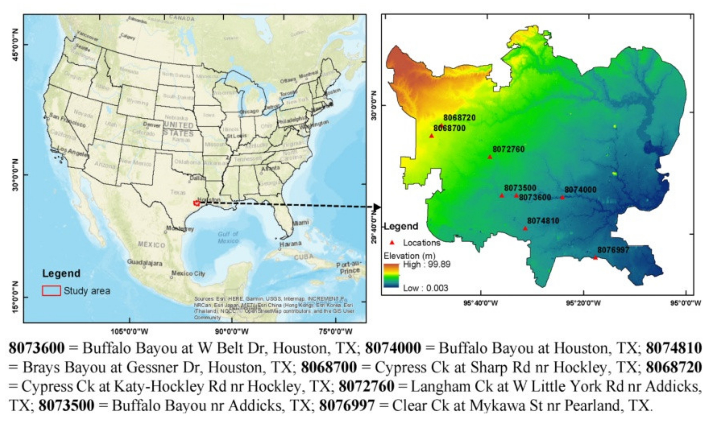
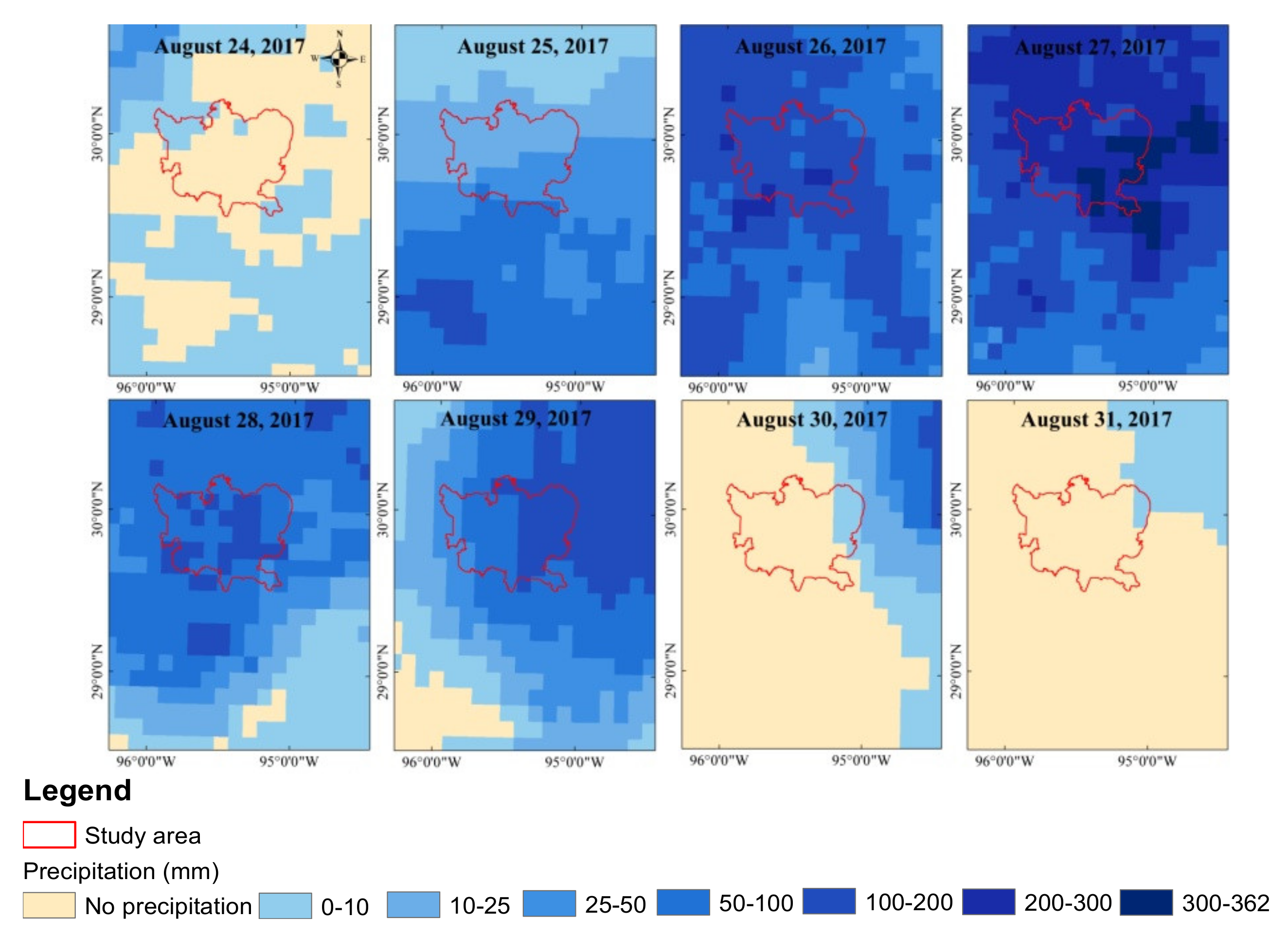
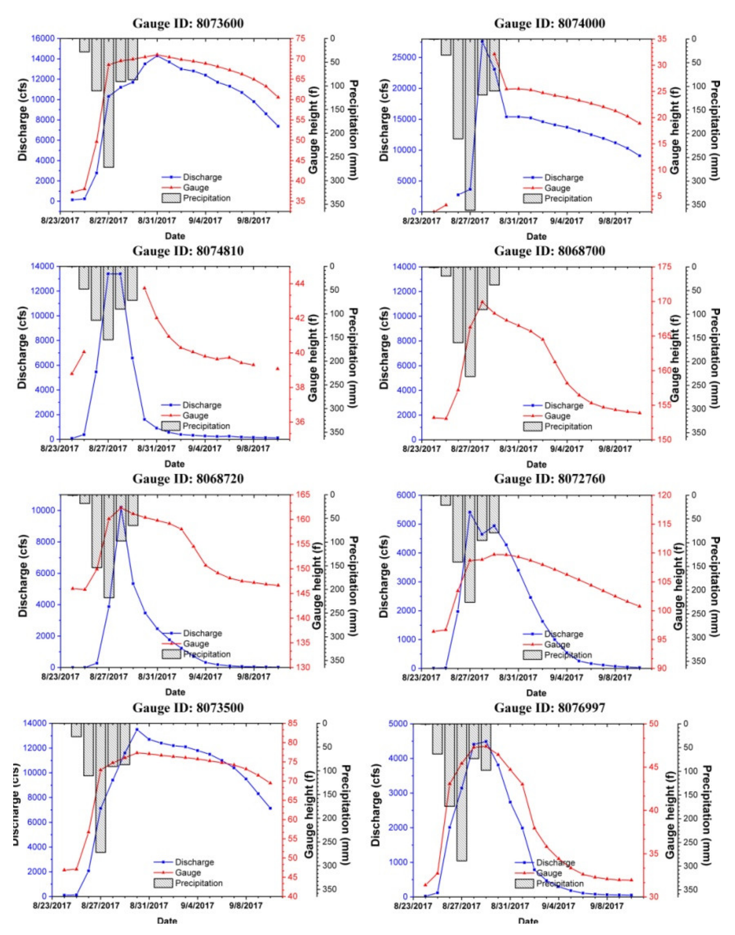
2.1. Site Properties and Conditions
2.2. Data and Processing
2.3. Estimation of Flood Depth Using Flood Extent and DEM
3. Results
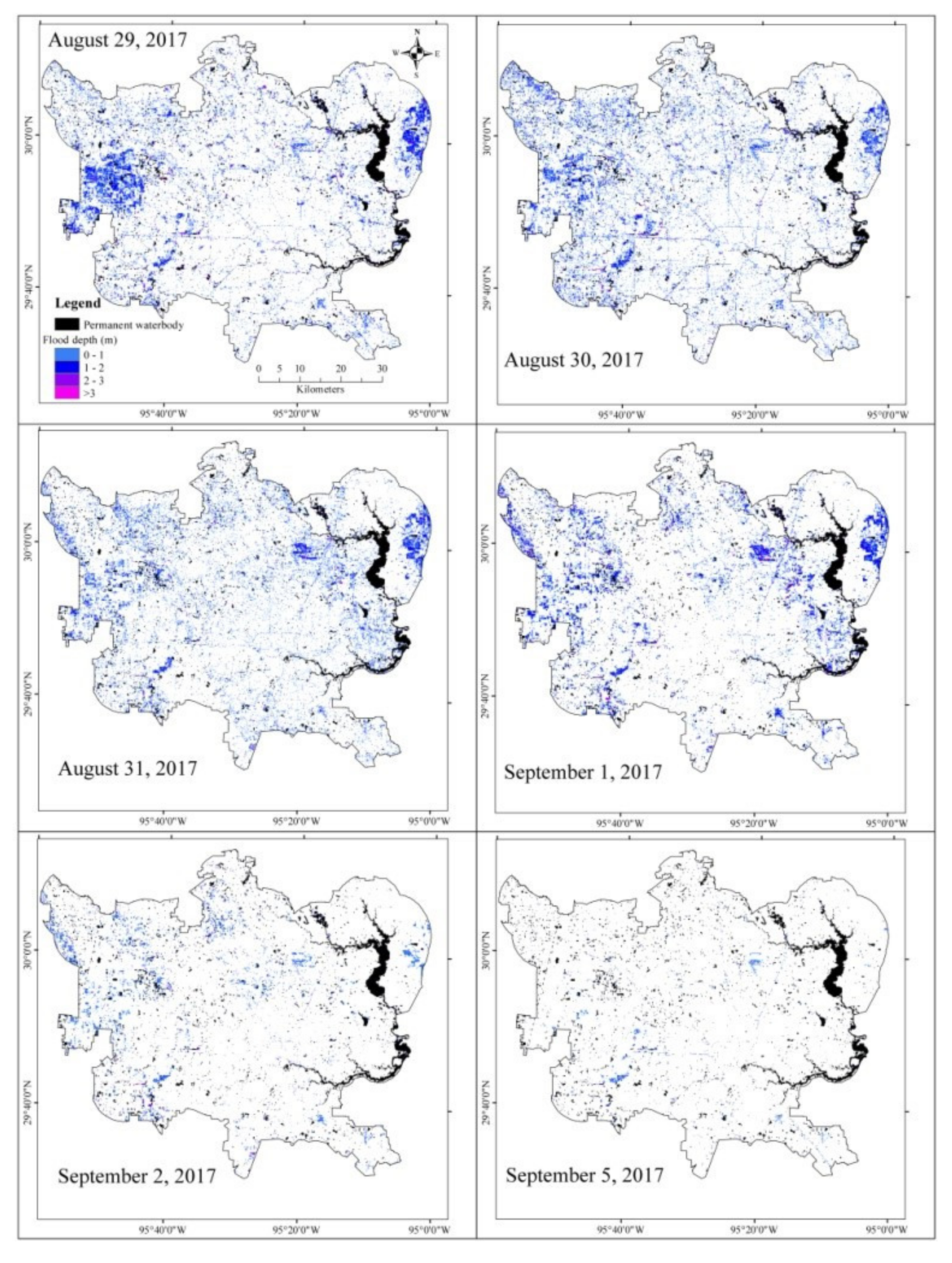
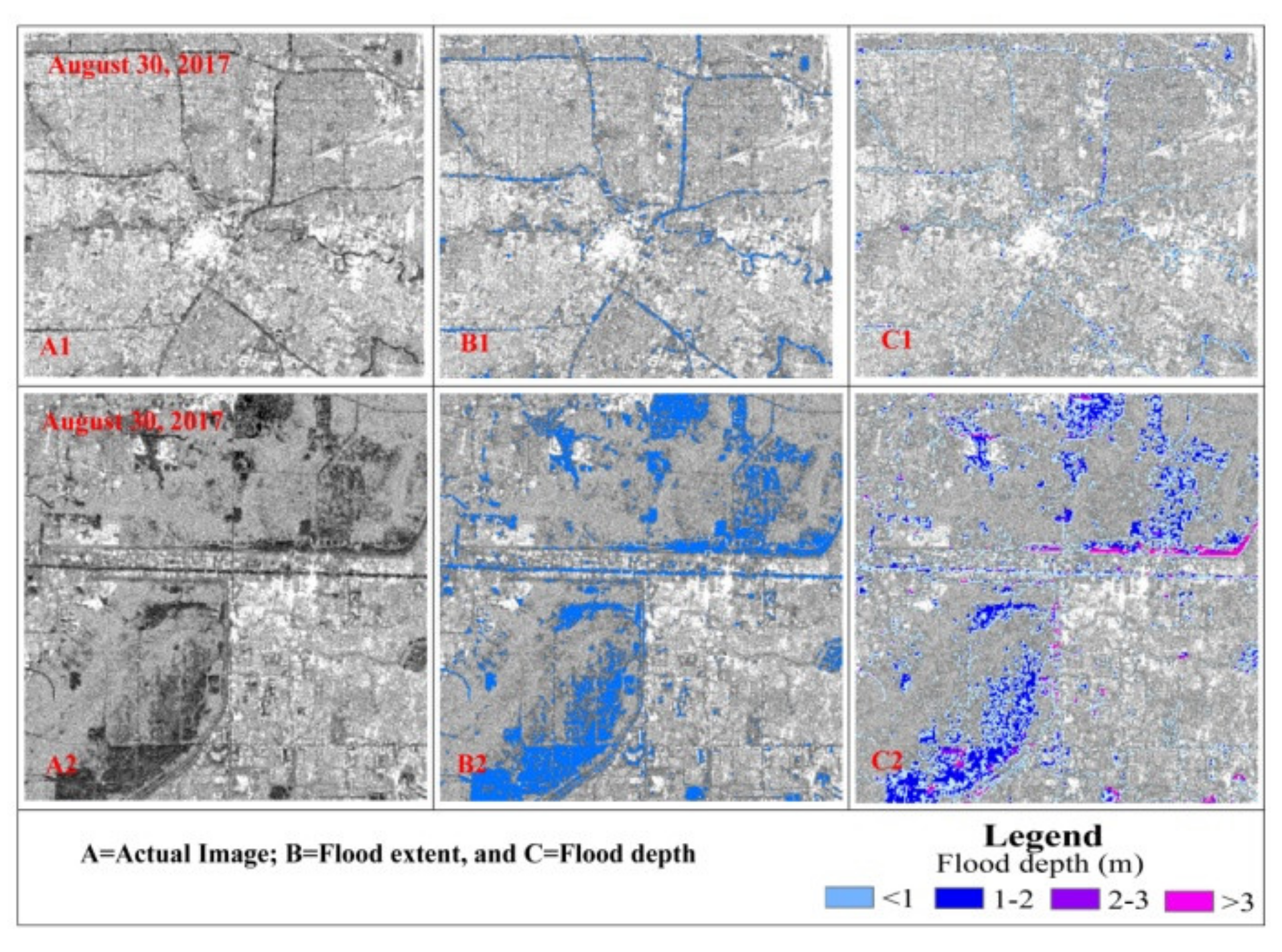
3.1. Flood Extent
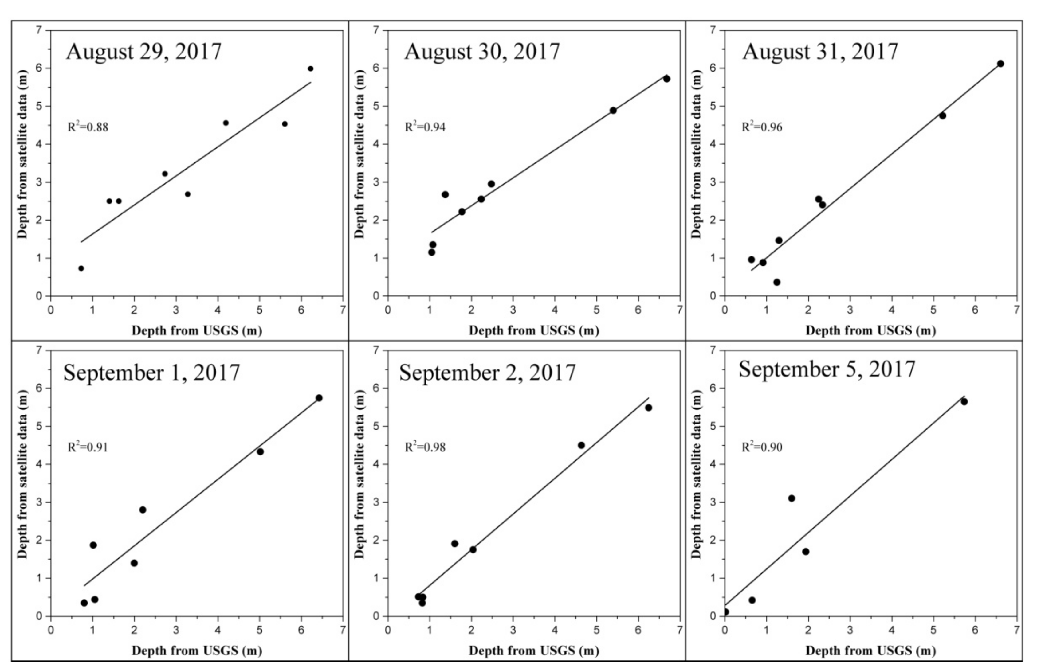
3.2. Flood Depth Estimation Using DEM
4. Conclusions
Author Contributions
Funding
Institutional Review Board Statement
Informed Consent Statement
Data Availability Statement
Acknowledgments
Conflicts of Interest
References
- Munich Re. NatCatSERVICE. 2018. Available online: https://natcatservice.munichre.com/ (accessed on 1 December 2020).
- NOAA National Centers for Environmental Information. U.S. 2020 Billion-Dollar Weather and Climate Disasters. 2020. Available online: https://www.ncdc.noaa.gov/billions/ (accessed on 1 December 2021).
- Smith, D.I. Flood damage estimation-a review of urban stage-damage curves and loss functions. Water SA 1994, 20, 231–238. [Google Scholar]
- Amitrano, D.; Di Martino, G.; Iodice, A.; Riccio, D.; Ruello, G. Unsupervised rapid flood mapping using sentinel-1 GRD SAR images. IEEE Trans. Geosci. Remote Sens. 2018, 56, 3290–3299. [Google Scholar] [CrossRef]
- Twele, A.; Cao, W.; Plank, S.; Martinis, S. Sentinel-1-based flood mapping: A fully automated processing chain. Int. J. Remote Sens. 2016, 37, 2990–3004. [Google Scholar] [CrossRef]
- Alsdorf, D.E.; Smith, L.C.; Melack, J.M. Amazon floodplain water level changes measured with interferometric sir-c radar. IEEE Trans. Geosci. Remote Sens. 2001, 39, 423–431. [Google Scholar] [CrossRef]
- Brown, K.M.; Hambidge, C.H.; Brownett, J.M. Progress in operational flood mapping using satellite synthetic aperture radar (sar) and airborne light detection and ranging (LiDAR) data. Prog. Phys. Geogr. 2016, 40, 196–214. [Google Scholar] [CrossRef]
- Van Oldenborgh, G.J.; van der Wiel, K.; Sebastian, A.; Singh, R.; Arrighi, J.; Otto, F.; Haustein, K.; Li, S.; Vecchi, G.; Cullen, H. Corrigendum: Attribution of extreme rainfall from hurricane Harvey, august 2017 (2017 Environ. Res. Lett. 12 124009). Environ. Res. Lett. 2018, 13, 019501. [Google Scholar] [CrossRef]
- Risser, M.D.; Wehner, M.F. Attributable human-induced changes in the likelihood and magnitude of the observed extreme precipitation during hurricane Harvey. Geophys. Res. Lett. 2017, 44, 12–457. [Google Scholar] [CrossRef] [Green Version]
- Emanuel, K. Assessing the present and future probability of Hurricane Harvey’s rainfall. Proc. Natl. Acad. Sci. USA 2017, 114, 12681–12684. [Google Scholar] [CrossRef] [Green Version]
- Sarkar, S.; Singh, R.P.; Chauhan, A. Anomalous changes in meteorological parameters along the track of 2017 Hurricane Harvey. Remote Sens. Lett. 2018, 9, 487–496. [Google Scholar] [CrossRef]
- Zhang, B.; Wdowinski, S.; Oliver-Cabrera, T.; Koirala, R.; Jo, M.; Osmanoglu, B. Mapping the extent and magnitude of severe flooding induced by Hurricane IRMA with multi-temporal SENTINEL-1 SAR and InSAR observations. Int. Arch. Photogramm. Remote Sens. Spatial Inf. Sci. 2018, 42, 2237–2244. [Google Scholar] [CrossRef] [Green Version]
- Plank, S.; Jüssi, M.; Martinis, S.; Twele, A. Mapping of flooded vegetation by means of polarimetric sentinel-1 and alos-2/palsar-2 imagery. Int. J. Remote Sens. 2017, 38, 3831–3850. [Google Scholar] [CrossRef]
- Lin, L.; Weng, F. Estimation of hurricane maximum wind speed using temperature anomaly derived from advanced technology microwave sounder. IEEE Geosci. Remote Sens. Lett. 2018, 15, 639–643. [Google Scholar] [CrossRef]
- NOAA. 2017. Available online: https://www.weather.gov/crp/hurricane_harvey (accessed on 1 March 2018).
- FEMA. Historic Disaster Response to Hurricane Harvey in Texas. 2017. Available online: www.fema.gov/news-release/2017/09/22/historicdisaster-response-hurricane-harvey-texas (accessed on 1 March 2018).
- Jonkman, S.N.; Godfroy, M.; Sebastian, A.; Kolen, B. Brief communication: Loss of life due to hurricane Harvey. Nat. Hazards Earth Syst. Sci. 2018, 18, 1073–1078. [Google Scholar] [CrossRef] [Green Version]
- Millera, M.M.; Shirzaei, M. Land subsidence in Houston correlated with flooding from Hurricane Harvey. Remote Sens. Environ. 2019, 225, 368–378. [Google Scholar] [CrossRef]
- Huang, X.; Runkle, B.R.K.; Isbell, M.; Moreno-García, B.; McNairn, H.; Reba, M.L.; Torbick, N. Rice inundation assessment using polarimetric UAVSAR data. Earth Space Sci. 2021, 8, e2020EA001554. [Google Scholar] [CrossRef]
- Brisco, B.; Short, N.; van der Sanden, J.; Landry, R.; Raymond, D. A semi-automated tool for surface water mapping with radarsat-1. Can. J. Remote Sens. 2009, 35, 336–344. [Google Scholar] [CrossRef]
- López-Caloca, A.A.; Tapia-Silva, F.O.; Rivera, G. Sentinel-1 satellite data as a tool for monitoring inundation areas near urban areas in the Mexican tropical wet. In Water Challenges of an Urbanizing World; IntechOpen: London, UK, 2018; p. 127. [Google Scholar]
- Manjusree, P.; Kumar, L.P.; Bhatt, C.M.; Rao, G.S.; Bhanumurthy, V. Optimization of threshold ranges for rapid flood inundation mapping by evaluating backscatter profiles of high incidence angle sar images. Int. J. Disaster Risk Sci. 2012, 3, 113–122. [Google Scholar] [CrossRef] [Green Version]
- Yésou, H.; Huber, C.; Haouet, S.; Lai, X.; Huang, S.; de Fraipont, P.; Desnos, Y.L. Exploiting sentinel 1 time series to monitor the largest fresh water bodies in pr china, the Poyang lake. In Proceedings of the 2016 IEEE International Geoscience and Remote Sensing Symposium (IGARSS), Beijing, China, 10–15 July 2016; pp. 3882–3885. [Google Scholar]
- Huffman, G.J.; Bolvin, D.T.; Nelkin, E.J. Day 1 IMERG Final Run Release Notes; NASA/GSFC: Greenbelt, MD, USA, 2015; p. 9. [Google Scholar]
- Cohen, S.; Brakenridge, G.R.; Kettner, A.; Bates, B.; Nelson, J.; McDonald, R.; Huang, Y.F.; Munasinghe, D.; Zhang, J. Estimating floodwater depths from flood inundation maps and topography. JAWRA J. Am. Water Resour. Assoc. 2018, 54, 847–858. [Google Scholar] [CrossRef]
- Huang, F.; Cao, Z.; Guo, J.; Jiang, S.; Li, S.; Guo, Z. Comparisons of heuristic, general statistical and machine learning models for landslide susceptibility prediction and mapping. Catena 2020, 191, 104580. [Google Scholar] [CrossRef]
- Janowski, L.; Tylmann, K.; Trzcinska, K.; Rudowski, S.; Tegowski, J. Exploration of Glacial Landforms by Object-Based Image Analysis and Spectral Parameters of Digital Elevation Model. IEEE Trans. Geosci. Remote Sens. 2021, 60, 4502817. [Google Scholar] [CrossRef]
- Middleton, M.; Nevalainen, P.; Hyvönen, E.; Heikkonen, J.; Sutinen, R. Pattern recognition of LiDAR data and sediment anisotropy advocate a polygenetic subglacial mass-flow origin for the Kemijärvi hummocky moraine field in northern Finland. Geomorphology 2020, 362, 107212. [Google Scholar] [CrossRef]
- Gebremichael, E.; Molthan, A.L.; Bell, J.R.; Lori, A.S.; Hain, C. Flood Hazard and Risk Assessment of Extreme Weather Events Using Synthetic Aperture Radar and Auxiliary Data: A Case Study. Remote Sens. 2020, 12, 3588. [Google Scholar] [CrossRef]
- Hashemi, H.; Nordin, M.; Lakshmi, V.; Huffman, G.J.; Knight, R. Bias correction of long-term satellite monthly precipitation product (TRMM 3b43) over the conterminous United States. J. Hydrometeorol. 2017, 18, 2491–2509. [Google Scholar] [CrossRef]
- Mondal, A.; Lakshmi, V.; Hashemi, H. Intercomparison of trend analysis of multisatellite monthly precipitation products and gauge measurements for river basins of India. J. Hydrol. 2018, 565, 779–790. [Google Scholar] [CrossRef]
- Le, M.-H.; Lakshmi, V.; Bolten, J.; Bui, D.D. Adequacy of satellite-derived precipitation estimate for hydrological modeling in Vietnam basins. J. Hydrol. 2020, 586, 124820. [Google Scholar] [CrossRef]
- Lakshmi, V.; Fayne, J.; Bolten, J. A comparative study of available water in the major river basins of the world. J. Hydrol. 2018, 567, 510–532. [Google Scholar] [CrossRef]
- Kansara, P.; Lakshmi, V. Estimation of land-cover linkage to trends in hydrological variables of river basins in the Indian sub-continent using satellite observation and model outputs. J. Hydrol. 2021, 603, 126997. [Google Scholar] [CrossRef]
- Dandridge, C.; Fang, B.; Lakshmi, V. Downscaling of smap soil moisture in the Lower Mekong river Basin. Water 2020, 12, 56. [Google Scholar] [CrossRef] [Green Version]
- Fang, B.; Lakshmi, V.; Bindlish, R.; Jackson, T. AMSR2 soil moisture downscaling using temperature and vegetation data. Remote Sens. 2018, 10, 1575. [Google Scholar] [CrossRef] [Green Version]
- Fang, B.; Lakshmi, V.; Bindlish, R.; Jackson, T.J. Downscaling of smap soil moisture using land surface temperature and vegetation data. Vadose Zone J. 2018, 17, 1–15. [Google Scholar] [CrossRef] [Green Version]
- Fang, B.; Lakshmi, V.; Jackson, T.J.; Bindlish, R.; Colliander, A. Passive/active microwave soil moisture change disaggregation using smapvex12 data. J. Hydrol. 2019, 574, 1085–1098. [Google Scholar] [CrossRef] [PubMed]
- Fang, B.; Lakshmi, V.; Bindlish, R.; Jackson, T.; Liu, P. Evaluation and Validation of a High Spatial Resolution Satellite Soil Moisture Product over the Continental United States. J. Hydrol. 2020, 588, 125043. [Google Scholar] [CrossRef]
- Fang, B.; Kansara, P.; Dandridge, C.; Lakshmi, V. Drought monitoring using high spatial resolution soil moisture data over Australia in 2015–2019. J. Hydrol. 2021, 594, 125960. [Google Scholar] [CrossRef]


| Properties | Sentinel-1 (29–30 August and 5 September) | UAVSAR (31 August and 1–2 September) | LiDAR DEM |
|---|---|---|---|
| Resolution | 5 × 20 m (range × azimuth) | 1.8 m × 0.8 m (range × azimuth) | 1 m (spatial resolution) |
| Swath width | 250 (IWS) km | 16 km | |
| Polarization | VV and VH | Full quad-polarization | |
| Organization | ESA | NASA | |
| Band | C | L |
| Depth of Floodwater | 29 August | 30 August | 31 August | 1 September | 2 September | 5 September |
|---|---|---|---|---|---|---|
| Depth below 1 m in respect to total area (%) | 8.19 | 10.13 | 9.12 | 6.75 | 3.23 | 1.14 |
| Depth below 2 m in respect to total area (%) | 10.90 | 12.21 | 10.70 | 9.28 | 3.60 | 1.21 |
| Total flooded area | 11.70 | 12.92 | 11.09 | 10.00 | 3.82 | 1.30 |
| Type | 29 August | 30 August | 31 August | 1 September | 2 September | 5 September |
|---|---|---|---|---|---|---|
| Overall accuracy | 0.96 | 0.96 | 1 | 1 | 0.96 | 1 |
| Kappa | 0.91 | 0.91 | 1 | 1 | 0.90 | 1 |
Publisher’s Note: MDPI stays neutral with regard to jurisdictional claims in published maps and institutional affiliations. |
© 2022 by the authors. Licensee MDPI, Basel, Switzerland. This article is an open access article distributed under the terms and conditions of the Creative Commons Attribution (CC BY) license (https://creativecommons.org/licenses/by/4.0/).
Share and Cite
Kundu, S.; Lakshmi, V.; Torres, R. Flood Depth Estimation during Hurricane Harvey Using Sentinel-1 and UAVSAR Data. Remote Sens. 2022, 14, 1450. https://doi.org/10.3390/rs14061450
Kundu S, Lakshmi V, Torres R. Flood Depth Estimation during Hurricane Harvey Using Sentinel-1 and UAVSAR Data. Remote Sensing. 2022; 14(6):1450. https://doi.org/10.3390/rs14061450
Chicago/Turabian StyleKundu, Sananda, Venkat Lakshmi, and Raymond Torres. 2022. "Flood Depth Estimation during Hurricane Harvey Using Sentinel-1 and UAVSAR Data" Remote Sensing 14, no. 6: 1450. https://doi.org/10.3390/rs14061450